Article

A Family of C0 Quadrilateral Plate Elements Based on the Refined Zigzag Theory for the Analysis of Thin and Thick Laminated Composite and Sandwich Plates

Department of Mechanical and Aerospace Engineering, Politecnico di Torino, 10129 Torino, Italy
*
Author to whom correspondence should be addressed.
J. Compos. Sci. 2019, 3(4), 100; https://doi.org/10.3390/jcs3040100
Submission received: 14 October 2019 / Revised: 13 November 2019 / Accepted: 14 November 2019 / Published: 16 November 2019
(This article belongs to the Special Issue Feature Papers in Journal of Composites Science in 2019)

Abstract

:
The present work focuses on the formulation and numerical assessment of a family of C0 quadrilateral plate elements based on the refined zigzag theory (RZT). Specifically, four quadrilateral plate elements are developed and numerically tested: The classical bi-linear 4-node element (RZT4), the serendipity 8-node element (RZT8), the virgin 8-node element (RZT8v), and the 4-node anisoparametric constrained element (RZT4c). To assess the relative merits and drawbacks, numerical tests on bending (maximum deflection and stresses) and free vibration analysis of laminated composite and sandwich plates under different boundary conditions and transverse load distributions are performed. Convergences studies with regular and distorted meshes, transverse shear-locking effect for thin and very thin plates are carried out. It is concluded that the bi-linear 4-node element (RZT4) has performances comparable to the other elements in the range of thin plates when reduced integration is adopted but presents extra zero strain energy modes. The serendipity 8-node element (RZT8), the virgin 8-node element (RZT8v), and the 4-node anisoparametric constrained element (RZT4c) show remarkable performance and predictive capabilities for various problems, and transverse shear-locking is greatly relieved, at least for aspect ratio equal to 5 × 10², without using any reduced integration scheme. Moreover, RZT4c has well-conditioned element stiffness matrix, contrary to RZT4 using reduced integration strategy, and has the same computational cost of the RZT4 element.

1. Introduction

In the last decades, multi-layered composite and sandwich structures have been increasingly used in different engineering fields (aerospace, automotive, marine, nuclear, and civil), thanks to their advantages over the traditional metallic structures due to their high specific stiffness and strength and their tailoring capabilities. Commonly built up with a sequence of layers of composite materials arranged thorough thickness, such structures typically exhibit a transverse shear deformability higher than their metallic counterpart, thus their structural analysis requires adequate models to take into account these effects.
In the framework of the displacement-based beam, plate, and shell theories, equivalent single layer (ESL) theories, where the displacement field is assumed smoothly continuous through-the-thickness, and layer-wise (LW) theories, where a local displacement field is assumed for each layer, are commonly used; see the recent review of Abrate and Di Sciuva [1,2]. Among the ESL theories, for engineering applications, the classical plate theory (CPT) is widely used especially for thin plates. In thick laminates, the shear deformability is no longer negligible and must be taken into account. Contrary to the CPT, the first-order shear deformation theory (FSDT), first formulated by Mindlin and extended to the heterogeneous anisotropic plates by Whitney and Pagano [3], allows the rotation of the normal to the reference surface to be independent of the slope of the reference surface. In the FSDT, the thickness-wise distribution of the transverse shear stresses in a multi-layered plate is a piecewise constant function, thus due to the step-wise variation of the transverse shear moduli along the thickness, it violates the continuity requirement of the transverse stresses at the interfaces and the vanishing transverse shear stresses conditions on the top and bottom surfaces of the plate. It also needs an appropriate shear correction factor due to the assumption of linear transverse shear stresses distribution along the plate thickness. Generally speaking, these models are not capable to predict the stress distributions along the thickness with acceptable accuracy, the range of their applicability being limited to compute the global responses, like maximum deflection, natural frequencies, and buckling loads [4]. To improve the accuracy of the estimates of the in-plane displacements and stresses distribution along the thickness, the higher-order shear deformation theories (HOSDT) are used. In the framework of HOSDT, polynomials, trigonometric, exponential, and hyperbolic expansions of the axial displacement are commonly used; see Abrate and Di Sciuva [1,2]. These theories are generally more accurate than FSDT and do not require the use of ad-hoc shear correction factors but are unable to satisfy the transverse shear stresses continuity condition at the layer interfaces. Moreover, from a computational point of view, finite elements based on such theories require C1 continuity shape functions for the transverse displacement [5,6,7,8,9], while FSDT element-based require only C0 continuity [4]. In LW theories, each layer has its own displacement fields, each independent from the others, which leads to a quasi-3D description of the displacement and stress fields. This assures a high degree of accuracy, but for laminates with several numbers of layers or complex structures, the computational cost of these theories can become prohibitive [10,11,12,13]. A compromise between the computational efficiency of ESL theories and the accuracy of LW theories is represented by the so-called zigzag theories (ZZT). In order to simulate the distortion of the normal and the step-wise distribution of the transverse shear stresses along the thickness typical of multi-layered structures, in the ZZT the in-plane displacements are written as a superposition of a through-the-thickness polynomial distribution (global contribution such as in the ESL theories) and a piecewise linear continuous function, (local or zigzag contribution). Unlike the LW theories, the kinematics of ZZT has a fixed number of kinematic unknown variables, independent on the number of material layers. Generally, the ZZ theories provide more accurate response predictions for relatively thick laminated composite and sandwich structures than the corresponding ESL theories, and generally comparable to those given by LW theories, at a lower computational cost. The first to investigate displacement-based zigzag theories was Di Sciuva [14,15,16]. From a computational point of view, the main drawback of the classical ZZT is that the finite element formulation requires C1 shape functions, according to Di Sciuva [17,18,19,20]. In order to develop a zigzag theory free of the drawbacks of classical Di Sciuva’s ZZ theory, Tessler et al. [21,22,23,24] developed the refined zigzag theory (RZT) for beams, plates, and shells. The reader interested in a comparison of the performances and range of applicability of various zigzag functions is invited to read the paper of Gherlone [25]. From a computational point of view, the formulation of finite elements based on the RZT requires only C0 continuity of shape functions [26,27,28,29,30,31,32,33,34,35,36,37,38]. Although C0-continous elements are the most-widely used in commercial finite element software due to their computational efficiency, it is well known that overstiff unrealistic numerical results are obtained when using the conventional low-order isoparametric C0 finite elements (bi-linear shape functions for both deflection and bending rotation) in the analysis of thin and very thin plates; this phenomenon is known in the literature as the transverse shear-locking effect, according to Oñate [38,39,40].
There are many approaches to overcome this difficulty.
Generally, using higher-order isoparametric shape functions alleviates the shear-locking problem, but the computational cost increases. Therefore, higher-order elements are not well-suited for the nonlinear analysis (post-buckling analysis, transient nonlinear analysis, crash simulation, etc.) and failure analysis [41,42].
One of the more successful strategy of overcoming this problem in the 4-node bi-linear isoparametric plate element is to use the procedure commonly known as the reduced/selective integration technique to compute the transverse shear strain energy [38,43,44,45,46].
Unfortunately, there is an undesirable effect associated with this scheme, i.e., there may be instances where extra zero strain energy modes will appear.
Other strategies investigated in the open literature are based on the penalty constraints [38]. Among these, the discrete penalty constraints, such as the discrete Kirchhoff theory (DKT) [47,48], where the transverse shear strain energy is neglected in the formulation and the Kirchhoff assumption of zero transverse shear strains are imposed at specific discrete points in the element are commonly used; the mixed interpolation of tensorial components (MITC) strategy [49,50], in which ad hoc chosen strain fields are tied to the displacement-based strains; B-bar method [51]; and F-bar method [52,53], which relies on the concept of deviatoric/volumetric split and the replacement of the compatible deformation gradient with an assumed modified counterpart.
Another strategy is the assumed natural strain (ANS) method [49,54], which consists of interpolating the strain field at a set of chosen points, known as tying points, where the strain values coming from the quadrature points are replaced, in a weighted manner, by assumed strains. A synergic use of the DKT and ASN strategies can be found in References [55,56]; the discrete shear gap (DSG) method [57], where the discretized shear gap field is determined by the interpolation of the nodal shear gaps. The anisoparametric interpolation strategy was proposed by Tessler et al. [58] for beam finite element and by Tessler [59] for plate elements. It requires that the shape functions for the transverse deflection be a complete polynomial one degree higher than the shape functions used to interpolate the bending rotations. This element was named anisoparametric virgin element [58]. To achieve simple nodal patterns, the constraint condition of constant effective transverse shear strain along the edges of the element is imposed. This allows one to eliminate the extra degree of freedom in the transverse deflection. The resulting element is named constrained anisoparametric, and it is simple, variationally consistent, and, more interestingly, computationally efficient.
This strategy was successfully applied to the formulation of beam, plate, and shell elements, [58,59,60,61,62,63,64,65,66,67]. Recently, Gherlone et al. [26] and Di Sciuva et al. [34] formulated beams elements based on the RZT using the constrained anisoparametric strategy. In Versino et al. [28], the approach has been used to formulate triangular shell elements. The numerical assessment shows how these new elements can alleviate the shear-locking phenomenon using the full integration (i.e., “full” Gaussian quadrature).
In the present work, the attention is focused on the formulation, implementation, and numerical assessment of a family of C0 quadrilateral plate elements based on RZT, with special emphasis on their numerical performances not only for thick, but also for thin and very thin plates. Using full integration Gaussian quadrature scheme the stiffness and mass matrices and nodal loads vector are computed. This work is an extension to the plate of the approach successfully applied to the beam in Gherlone et al. [26] and Di Sciuva et al. [34].
The first two elements of the family (RZT4 and RZT8) are isoparametric quadrilateral plate elements. RZT4 is a 4-node element with bilinear shape functions; RZT8 is an 8-node element with quadratic serendipity shape functions. Each node has seven degrees of freedom (dof’s): Three displacements (u1, u2, w), two bending rotations (θ1, θ2), and two amplitudes of the zigzag functions, (ψ1, ψ2). The third one, named RZT8v (v stands for virgin), is an anisoparametric quadrilateral plate element, i.e., it is an RZT4 plate element for the six kinematic variables (u1, u2, θ1, θ2, ψ1, ψ2) and a RZT8 plate element for the transverse displacement, w. The last one, named RZT4c, is a 4-node anisoparametric constrained element. It is obtained from the RZT8v element by imposing the constraint condition of constant effective transverse shear strain along the edges of the element.
To numerically assess the relative merits of these four C0 plate elements, in particular, of the RZT4c element, several cases are examined. Convergences studies and parametric investigations, under various boundary conditions and transverse pressure distribution, with regular and distorted meshes, are carried out by considering static and free vibration problems.
It is concluded that the bi-linear 4-node element (RZT4) has performances comparable to the other elements in the range of thin plates when reduced integration is adopted but presents extra zero strain energy modes. The serendipity 8-node element (RZT8), the virgin 8-node element (RZT8v), and the 4-node anisoparametric constrained element (RZT4c) show remarkable performance and predictive capabilities, at a reduced computational cost, for various problems, and the transverse shear-locking is greatly relieved without using any reduced integration schemes, for thin plate (aspect ratio equal to 5 × 10²), at least for 8 × 8 mesh. Moreover, RZT4c has well-conditioned element stiffness matrix, contrary to RZT4 using reduced integration strategy, and the same computational cost.

2. Theoretical Basis of Refined Zigzag Theory (RZT) and Finite Element Modeling

We consider a rectangular multilayered flat plate of length a, width b, and total thickness h, assumed constant (Figure 1). It is composed of a finite number N of orthotropic elastic layers of uniform thickness perfectly bonded together. The material of each layer is assumed to have a plane of elastic symmetry parallel to the reference surface (here chosen to be the midsurface of the plate) and principal orthotropy directions arbitrarily oriented with respect to the laminate reference frame (x1, x2).
The points of the plate are referred to an orthogonal Cartesian co-ordinate system X = { x j }   ( j = 1 , 2 , 3 ) , where x = { x β }   ( β = 1 , 2 ) is the set of in-plane co-ordinates on the reference plane, and x 3 z is the co-ordinate normal to the reference plane (Figure 1); the origin of the reference frame is fixed at the center of the middle-plane of the plate. So, x 1 ( a 2 , + a 2 ) , x 2 ( b 2 , + b 2 ) , and x 3 ( h 2 , + h 2 ) .
If not otherwise stated, the superscript (k) is attached to quantities of the kth layer (k = 1, N), whereas the subscript (k) is attached to quantities evaluated at the kth interface (k = 1, N − 1) between the k and (k + 1) layer. Also, we use the subscript b and t to indicate the top and bottom surfaces of the plate. For example, z ( 0 ) = z b = h 2 , z ( N ) = z t = + h 2 and h ( k ) = z ( k ) z ( k 1 )   ( k = 1 , 2 , , N ) (see Figure 1 and Figure 2). The symbol ( ) , i = ( ) x i refers to the partial derivative of the function ( ) with respect to the coordinate x i ; a dot over a quantity refers to the partial derivative with respect to time of that quantity. Finally, the Einsteinian summation convention over repeated indices is adopted, with Latin indices ranging from 1 to 3, and Greek indices ranging from 1 to 2.
The displacement field at time t in the RZT theory can be written as
d ˜ ( x j , t ) = Z d ( z ) d ( x β , t )
where
d ˜ ( x j , t ) = { u ˜ 1 ( x j , t ) u ˜ 2 ( x j , t ) u ˜ 3 ( x j , t ) } = { u ˜ ( x j , t ) u ˜ 3 ( x j , t ) }
is the vector of the displacement components of the generic point belonging to the plate and u ˜ ( x j , t ) is the vector of the in-plane displacement components. As usual in the plate theory, the transverse displacement is assumed to be constant along the thickness, i.e., u ˜ 3 ( x j , t ) = u 3 ( x β , t ) = w ( x β , t ) . In the refined zigzag theory, the in-plane kinematics is based on the superposition of a global (G) firs-order kinematics (that of the FSDT plate theory) and a local (L) layer-wise correction of the in-plane displacements (see, Figure 2). Thus, the in-plane displacement field at time t is assumed to be (see Figure 2)
u ˜ ( x j , t ) = { u ˜ 1 ( x j , t ) u ˜ 2 ( x j , t ) } = u G ( x j , t ) + u L ( x j , t )
where
u G ( x j , t ) = { u ˜ 1 G ( x j , t ) u ˜ 2 G ( x j , t ) } = u ( x β , t ) + z θ ( x β , t )
gives the contribution, which is continuous with its first derivatives with respect to the z-coordinate (the global (G), contribution of the first-order kinematics) and
u L ( k ) ( x j , t ) = { u ˜ 1 L ( k ) ( x j , t ) u ˜ 2 L ( k ) ( x j , t ) } = ϕ ( k ) ( z ) ψ ( x β , t )
gives the local (L), contribution to the in-plane displacement, which is continuous with respect to z, but with jumps in the first derivative at the interfaces between adjacent layers. In Equations (4) and (5),
u ( x β , t ) = { u 1 ( x β , t ) u 2 ( x β , t ) } , θ ( x β , t ) = { θ 1 ( x β , t ) θ 2 ( x β , t ) } , ψ ( x β , t ) = { ψ 1 ( x β , t ) ψ 2 ( x β , t ) } ,   ϕ ( k ) = [ ϕ 1 ( k ) ( z ) 0 0 ϕ 2 ( k ) ( z ) ]
where u 1 and u 2 are the displacements along the x 1 and x 2 axis of a point belonging to the middle plane of the plate; θ 1 and θ 2 are the bending rotation of the normal to the middle surface along the directions + x 2 and x 1 , respectively; ψ 1 and ψ 2 represent the spatial amplitudes of the zigzag functions ϕ 1 ( k ) and ϕ 2 ( k ) , respectively. It should be noted that FSDT is a special case of the RZT, i.e., RZT reduces to FSDT when u L ( k ) = 0 (see Equations (1) and (2)). By taking into account these definitions, in Equation (1)
d = { u 1 u 2 u 3 θ 1 θ 2 ψ 1 ψ 2 } = { d m w d r } ; d m = u = { u 1 u 2 } ; d r = { d θ d ψ } ; d θ = θ = { θ 1 θ 2 } ; d ψ = ψ = { ψ 1 ψ 2 }
Z d ( z ) = [ I 0 z I ϕ ( k ) 0 1 0 0 ] .
For the k th layer of thickness h ( k ) , the refined zigzag functions have the following expressions [34]:
ϕ 1 ( k ) ( z ) = ( z + h 2 ) ( G 4 Q ¯ 44 ( k ) 1 ) + q = 2 k h ( q 1 ) ( G 4 Q ¯ 44 ( q 1 ) G 4 Q ¯ 44 ( k ) ) ϕ 2 ( k ) ( z ) = ( z + h 2 ) ( G 5 Q ¯ 55 ( k ) 1 ) + q = 2 k h ( q 1 ) ( G 5 Q ¯ 55 ( q 1 ) G 5 Q ¯ 55 ( k ) )   ( k = 1 , , N )
where
1 G j = 1 h k = 1 N z b ( k ) z t ( k ) d z Q ¯ j j ( k ) j = 4 , 5
and Q ¯ j j ( k ) is the transformed reduced transverse shear stiffness modulus of the kth layer (see Equation (22)).
Equations (9) and (10) show that the refined zigzag functions ϕ α ( k ) are a-priori known piecewise continuous functions of z, depend only on the thickness and transverse shear mechanical properties of the constituent layers, and vanish on the bottom ( z = h 2 ) and top ( z = + h 2 ) surfaces of the plate (see Figure 2).
In Equation (8) and in the body of the paper, I stands for the identity matrix and 0 for the null rectangular matrix, which dimensions follow from the rule of the matrix product and partitioning.

2.1. Virtual Work Principle and Discretized Equations of Motion

The discretized equations of motion are obtained via the dynamic version of the principle of virtual displacements (D’Alembert principle)
δ U δ W e x t = δ W i n
where ( δ is the variational operator) δ U is the virtual variation of the work done by the internal forces (stress); δ W i n is the virtual variation of the work done by the inertia forces, and δ W e x is the virtual variation of the work done by the applied forces.

2.1.1. Virtual Variation of the Strain Energy, δ U

The virtual variation of the work done by the internal stresses (strain energy) reads
δ U = a 2 + a 2 b 2 + b 2 δ ε ˜ T σ ˜ d x 1 d x 2
with
= s = 1 N x 3 ( s 1 ) x 3 ( s ) ( ) d x 3 .
In Equation (12), σ ˜ and ε ˜ are the vectors of stress and linearized strain components, respectively. By taking into account the assumed displacement field, Equation (1), and assuming, as usual in plate theory, σ ˜ 33 = 0 , yields
δ U = a 2 + a 2 b 2 + b 2 δ ( ε d ) T R d x 1 d x 2
where
R = Z ε T σ ˜ ( k )
is the vector of the stress and moment stress resultants for unit length,
R T = [ N T M T M ( ϕ ) T T T T ( ϕ ) T ]
( N , M , M ( ϕ ) ) = ( { Ν 11 Ν 22 Ν 12 } , { Μ 11 Μ 22 Μ 12 } , { M 11 ( ϕ ) M 21 ( ϕ ) M 12 ( ϕ ) M 22 ( ϕ ) } ) = ( 1 , z , Φ ( k ) ) σ ˜ p ( k )
( T , T ( ϕ ) ) = ( { T 1 T 2 } , { T 1 ( ϕ ) T 2 ( ϕ ) } ) = ( 1 , ϕ , 3 ( k ) ) σ ˜ t ( k )
σ ˜ ( k ) = { σ ˜ p ( k ) σ ˜ t ( k ) } , σ ˜ p ( k ) = { σ ˜ 11 σ ˜ 22 σ ˜ 12 } ( k ) , σ ˜ t ( k ) = { σ ˜ 13 σ ˜ 23 } ( k )
Z ε = [ I z I Φ ( k ) 0 0 0 0 0 I ϕ , 3 ( k ) ] , Φ ( k ) = [ ϕ 1 ( k ) 0 0 0 0 0 0 ϕ 2 ( k ) 0 ϕ 2 ( k ) ϕ 1 ( k ) 0 ] .
The constitutive equations for a generally orthotropic layer are
σ ˜ p ( k ) = Q ¯ p ( k ) ε ˜ p ( k ) ;   σ ˜ t ( k ) = Q ¯ t ( k ) γ ˜ ( k )
where
ε ˜ p ( k ) = { ε ˜ 11 ε ˜ 22 γ ˜ 12 } ( k ) = { u ˜ 1 , 1 u ˜ 2 , 2 u ˜ 1 , 2 + u ˜ 2 , 1 } ( k ) , γ ˜ ( k ) = { γ ˜ 13 γ ˜ 23 } ( k ) = { u ˜ 1 , 3 + w , 1 u ˜ 2 , 3 + w , 2 } ( k )
Q ¯ p ( k ) = [ Q ¯ 11 Q ¯ 12 Q ¯ 16 Q ¯ 12 Q ¯ 22 Q ¯ 26 Q ¯ 16 Q ¯ 26 Q ¯ 66 ] ( k ) , Q ¯ t ( k ) = [ Q ¯ 44 Q ¯ 45 Q ¯ 45 Q ¯ 55 ] ( k )
In Equation (22), Q ¯ i j ( k ) (i, j = 1, 2, 6) and Q ¯ i j ( k ) (i, j = 4, 5) are the plane stress transformed stiffness moduli of the kth layer, that are functions of the z-coordinate. Substituting Equations (20) and (22) into Equations (16) and (17) yields the plate constitutive equations in terms of the generalized displacements
R = S ( ε d )
with
S = Z ε T [ Q ¯ p 0 0 T Q ¯ t ] Z ε = [ A B A ϕ 0 0 B D B ϕ 0 0 A ϕ T B ϕ T D ϕ 0 0 0 0 0 A t B t ϕ 0 0 0 B t ϕ T D t ϕ ]
( A , B , D ) = ( 1 , z , z 2 ) Q ¯ p ( k ) ,   ( A ϕ , B ϕ , D ϕ ) = ( 1 , z , Φ ( k ) T ) Q ¯ p ( k ) Φ ( k ) ( A t , B t ϕ ) = ( 1 , ϕ , 3 ( k ) ) Q ¯ t ( k ) ,   D t ϕ = ϕ , 3 ( k ) T Q ¯ t ( k ) ϕ , 3 ( k )

2.1.2. Virtual Variation of the Inertia Forces, δ W i n

The virtual variation of the work done by the inertia forces reads
δ W i n = a 2 + a 2 b 2 + b 2 ρ d ˜ ¨ T δ d ˜ u ˜ d x 1 d x 2  
Substituting Equation (1) into Equation (26) yields
δ W i n = a 2 + a 2 b 2 + b 2 δ d T m d ¨ d x 1 d x 2  
where
m = ρ Z d T Z d = [ m ( 0 ) 0 m ( 1 ) m ϕ ( 0 ) 0 T m ( 0 ) 0 T 0 T m ( 1 ) T 0 m ( 2 ) m ϕ ( 1 ) m ϕ ( 0 ) T 0 m ϕ ( 1 ) T m ϕ ( 2 ) ]
( m ( 0 ) , m ( 1 ) , m ( 2 ) , m ϕ ( 0 ) , m ϕ ( 1 ) , m ϕ ( 2 ) ) = ρ ( I , z I , z 2 I , ϕ ( k ) , z ϕ ( k ) , ϕ ( k ) T ϕ ( k ) .

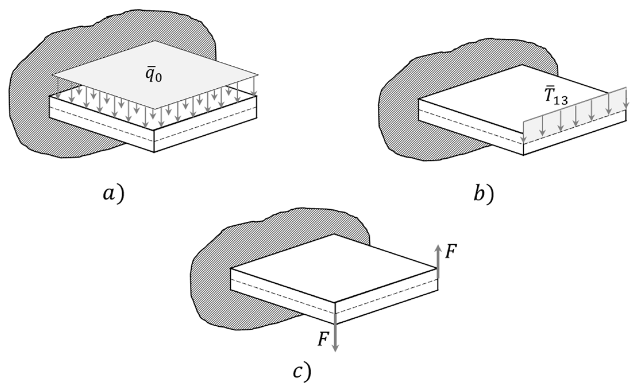
2.1.3. Virtual Variation of the Work of Applied Forces, δ W e x

δ W e x = a 2 + a 2 b 2 + b 2 q ¯ z δ w d x 1 d x 2 + + a 2 + a 2 ( T ¯ 23 ( x 1 , b 2 , t ) δ w ( x 1 , b 2 , t ) + T ¯ 23 ( x 1 , b 2 , t ) δ w ( x 1 , b 2 , t ) ) d x 1 + + b 2 + b 2 ( T ¯ 13 ( a 2 , x 2 , t ) δ w ( a 2 , x 2 , t ) + T ¯ 13 ( a 2 , x 2 , t ) δ w ( a 2 , x 2 , t ) ) d x 2
In writing Equation (30), it is assumed that the plate is subjected to a transverse pressure q ¯ z applied on the top surface of the plate, and to boundary transverse loads per unit length T ¯ α 3   ( α = 1 , 2 ) applied on the edge parallel to x α -axis.
Obviously,
δ W e x = 0
for free vibration.
In the previous equations, ρ ( x 3 ) is the material mass density and an overbar indicates the prescribed value of a quantity. The other symbols have been defined above.
Due to difficulty to obtain closed form solutions, we search for an approximate solution.

3. Finite Element Formulation

As is well known, the accuracy of the finite element solution depends on the ability of the assumed shape functions to accurately model the deformation modes of the structure.
In the following sections, several C0 quadrilateral plate elements derived using the displacement approach in conjunction with the RZT summarized in the previous Section will be described.

3.1. General Equation

Let us consider a general quadrilateral plate element with NN surrounding nodes. A generic 8-node (NN = 8) quadrilateral plate element is shown in Figure 3. The reference plane is the physical plane ( x 1 ,   x 2 ) . From a computational point of view, each element can be mapped in a conventional square element on the natural plane ( ξ ,   η ) where ( ξ ,   η ) ( 1 ,   1 ) , thus the numerical integration using the Gaussian quadrature can be easily implemented.
As usual in the finite element method, let us expand the vector of unknown generalized displacements (Equation (7)) of points belonging to element e in the form
d ( e ) ( ξ , η ; t ) = N ( e ) ( ξ , η ) q ( e ) ( t )
where q ( e ) ( t ) is the vector of the nodal degrees-of-freedom of the element e and N ( e ) ( ξ , η ) is the matrix of the element shape functions in the natural co-ordinates ( ξ , η ) .
In expanded format,
d ( e ) ( ξ , η ) = { d m ( e ) w ( 0 ) d r ( e ) } ( e ) = [ N m ( e ) 0 0 0 N w ( e ) 0 0 0 N r ( e ) ] { q m ( e ) q w ( e ) q r ( e ) } = N ( e ) q ( e ) .
d m ( e ) = N m ( e ) q m ( e ) = [ N u x ( e ) 0 0 N u y ( e ) ] { q u x ( e ) q u y ( e ) } ;    w ( 0 ) = N w ( e ) q w ( e ) ;    d r ( e ) = N r ( e ) q r ( e ) = [ N θ ( e ) 0 0 N ψ ( e ) ] { q θ ( e ) q ψ ( e ) } d θ ( e ) = N θ ( e ) q θ ( e ) = [ N θ x ( e ) 0 0 N θ y ( e ) ] { q θ x ( e ) q θ y ( e ) } ;    d ψ ( e ) = N ψ ( e ) q ψ ( e ) = [ N ψ ( e ) 0 0 N ψ ( e ) ] { q ψ ( e ) q ψ ( e ) }
In Equation (33), q i ( e ) ( t )   ( i u 1 , u 2 , w , θ 1 , θ 2 , ψ 1 , ψ 2 ) is the vector of the nodal dof’s of the generalized displacement “i” and N i ( e ) ( ξ , η ) is the matrix of the element shape functions for the same generalized displacement.
Substituting Equation (32) into Equations (13) and (27) and taking into account Equation (23) yields
δ U ( e ) = δ q ( e ) T K ( e ) q ( e )   ;   δ W i n ( e ) = δ q ( e ) T M ( e ) q ¨ ( e )
with
K ( e ) = 1 + 1 1 + 1 ( ε N ( e ) ) T S ( e ) ( ε N ( e ) ) J d ξ d η ;   M ( e ) = 1 + 1 1 + 1 N ( e ) T m ( e ) N ( e ) J d ξ d η .
Further (see, Equation (30)),
δ W e x ( e ) = δ q ( e ) T P ( e )
where
P ( e ) = 0
for free vibration;
P ( e ) T = 1 + 1 1 + 1 0 0 0 0 0 0 p ¯ 3 N ( e ) J d ξ d η + Γ p 0 0 0 0 0 0 T ¯ 3 N ( e ) d Γ
where
Γ p T ¯ 3 N ( e ) d Γ = a 2 + a 2 ( T ¯ 23 ( x 1 , b 2 ) N w ( x 1 , b 2 ) + T ¯ 23 ( x 1 , b 2 ) N w ( x 1 , b 2 ) ) d x 1 + + b 2 + b 2 ( T ¯ 13 ( a 2 , x 2 ) N w ( a 2 , x 2 ) + T ¯ 13 ( a 2 , x 2 ) N w ( a 2 , x 2 ) ) d x 2 = a 2 1 + 1 ( T ¯ 23 ( ξ , 1 ) N w ( ξ , 1 ) + T ¯ 23 ( ξ , 1 ) N w ( ξ , 1 ) ) d ξ + + b 2 1 + 1 ( T ¯ 13 ( 1 , η ) N w ( 1 , η ) + T ¯ 13 ( 1 , η ) N w ( 1 , η ) ) d η
for bending.
In Equations (26) and (39), J is the determinant of the Jacobian matrix of the co-ordinate transformation from the physical plane to the natural plane.

3.2. Shape Functions and Constrained Technique

From the variational statement used to derive the element governing equation, Equation (11), only the first derivatives of the kinematic variables appear in the virtual variation of the strain energy expression, Equation (13). Like FSDT, in formulating finite elements, refined zigzag theory (RZT) requires only C0 shape functions, which makes it attractive in formulating beams, plate, and shell elements [38].
In this Section, the attention is focused on the formulation of the shape functions of a family of C0 quadrilateral plate element based on RZT.
Table 1 summarizes the topology and the shape functions of the developed family of C0 quadrilateral plate elements. The first two (RZT4 and RZT8) are isoparametric quadrilateral plate elements. RZT4 is a 4-node element with bilinear shape functions; RZT8 is an 8-node element with quadratic serendipity shape functions. Each node has seven dof’s: Three displacements (u1, u2, w), two bending rotations (θ1, θ2), and two amplitudes of the zigzag functions, (ψ1, ψ2) (see, Figure 1). For these elements, the same set of shape functions is used for approximating all the generalized displacements vector,
N u 1 ( e ) = N u 2 ( e ) = N w ( e ) = N θ 1 ( e ) = N θ 2 ( e ) = N ψ 1 ( e ) = N ψ 2 ( e )
As well known, a drawback of low-order C0 finite elements (bi-linear shape functions for both deflection and bending rotation) coupled with the full Gaussian quadrature to compute exactly the integrals of the element matrices, is the shear-locking effect. To eliminate shear-locking, reduced integration strategy is often used. Unfortunately, there is an undesirable effect associated with this scheme, i.e., there may be instances where extra zero strain energy modes will appear.
Tessler and Dong [58], for the Timoshenko beam element, identified the reason of shear-locking effect in the Kirchhoff constraints of the shear strain measure for very thin structures. As a possible solution, they proposed to use the anisoparametric interpolation, where the deflection w is approximated by a polynomial with one order of degree higher than the others used for the remaining kinematic variable (bending rotation, θ). These elements, named Virgin elements by Tessler and Dong [58], have one extra node in the middle beam point having only the w-dof. This approach has been extensively used to formulate C0 beam elements based on the RZT in Gherlone et al. [26] and Di Sciuva et al. [34]. When the anisotropic interpolation scheme is applied to quadrilateral plate elements, the shape functions are bilinear for all kinematic variables except for the transverse displacement, for which the 8-node serendipity shape functions are used, i.e., the extra node in the middle point of each edges have only the w-dof (see, Table 1 and Figure 4). This plate element is named RZT8v (v stands for virgin) in Table 1: It is an RZT4 plate element for the six kinematic variables (u1, u2, θ1, θ2, ψ1, ψ2) and an RZT8 plate element for the transverse displacement, w. Therefore, the shape function matrices for the RZT8v element read (see Table 1)
N L ( e ) = N u 1 ( e ) = N u 2 ( e ) = N θ 1 ( e ) = N θ 2 ( e ) = N ψ 1 ( e ) = N ψ 2 ( e ) = L 1 L 2 L 3 L 4
N w ( e ) = N 1 N 2 N 3 N 4 N 5 N 6 N 7 N 8 = N w r ( e ) N w o ( e )   N w r ( e ) = P 1 P 2 P 3 P 4 ; N w o ( e ) = P 5 P 6 P 7 P 8
The vector of the nodal transverse displacements can be split in two subvectors
q w ( e ) T = w 1 ( e ) w 2 ( e ) w 3 ( e ) w 4 ( e ) w 5 ( e ) w 6 ( e ) w 7 ( e ) w 8 ( e ) = q w r ( e ) T q w o ( e ) T q w r ( e ) T = w 1 ( e ) w 2 ( e ) w 3 ( e ) w 4 ( e ) ; q w o ( e ) T = w 5 ( e ) w 6 ( e ) w 7 ( e ) w 8 ( e )

Constrained Technique

The last one, named RZT4c in Table 1, is a 4-node anisoparametric constrained element (RZT4c). It is obtained from the RZT8v element applying the constrained-edge-strategy, as suggested by Tessler and Dong [58] and Tessler and Hughes [60,62], i.e., by imposing the constraint condition of constant effective transverse shear strain along the edges of the element.
For the FSDT, it is possible to refer either to the transverse shear strains ( γ 13 and γ 23 ) or to the transverse shear stress resultants ( T 1 and T 2 ) using the following relations.
T 1 = τ 13 ( k ) = A 44 ( w , 1 + θ 1 ) γ 13 = V 1 A 44 = ( w , 1 + θ 1 ) T 2 = τ 23 ( k ) = A 55 ( w , 2 + θ 2 ) γ 23 = V 2 A 55 = ( w , 2 + θ 2 )
Considering the RZT, the previous relations (Equation (45)) have an additional term (see Equations (17), (24), and (25))
T 1 = τ 13 ( k ) = A 44 ( w , 1 + θ 1 ) + B 44 ϕ ψ 1 γ 13 e f f = T 1 A 44 = ( w , 1 + θ 1 ) + r L ψ 1 T 2 = τ 23 ( k ) = A 55 ( w , 2 + θ 2 ) + B 55 ϕ ψ 2 γ 23 e f f = T 2 A 55 = ( w , 2 + θ 2 ) + r T ψ 2
where
r L = B 44 ϕ A 44 = β 1 ( k ) G 13 ( k ) G 13 ( k ) ; r T = B 55 ϕ A 55 = β 2 ( k ) G 23 ( k ) G 23 ( k ) .
It has been shown by Gherlone et al. [26] and by Di Sciuva et al. [34] that these two non-dimensional transverse-shear-parameters have a range of values r L , r T ( 1 , 0 ) , with r L , r T = 0 for homogeneous material properties through-the-thickness (when β α ( k ) = 0   α = 1 , 2 ), and r L , r T 1 for highly heterogeneous cross-sections, such as laminated composites and sandwiches. As said, to generate a constrained element from the virgin type element defined before, following Tessler and Dong [58] and Tessler and Hughes [60,62], we enforce along the edges of the element the following condition
γ s 3 , s e f f ( e ) = 0
i.e., constant effective transverse shear strain along the edges of the element. The transverse shear deformation along the edge can be expressed as
γ s 3 e f f = w , s + θ n + r ψ n
s is the coordinate running along an element edge; θ n ,   ψ n are the tangential edge rotation and the tangential zigzag amplitude, respectively; see Figure 5.
θ n = θ 1 cos α + θ 2 sin α ; ψ n = ψ 1 cos α + ψ 2 sin α
α is the angle between the direction s and x 1 axis,
γ s 3 e f f = w , s + θ 1 cos α + θ 2 sin α + r L ψ 1 cos α + r T ψ 2 sin α
Therefore, constraint (48) reads
γ s 3 , s e f f = w , s s + θ 1 , s cos α + θ 2 , s sin α + r L ψ 1 , s cos α + r T ψ 2 , s sin α = 0
The edge-coordinate is s ( l i j 2 , l i j 2 ) where l i j is the length of the edge defined by nodes i an j (see Figure 5). In the natural plane, the non-dimensional coordinate is ξ or η , in particular for the edges along the ξ direction ξ = 2 s l i j and for the edges along the η direction η = 2 s l i j .
Imposing constraint Equation (52) on the four edges of the plate elements yields the following set of four equations with q w o ( e ) as unknown
B w o ( e ) q w o ( e ) = [ B w r ( e ) B r ( e ) ] q w r ( e ) T q θ x ( e ) T q θ y ( e ) T q ψ x ( e ) T q ψ y ( e ) T T
where
B w o ( e ) = 1 2 N w o ( e ) , ξ ξ | η = 1 N w o ( e ) , ξ ξ | η = + 1 N w o ( e ) , η η | ξ = 1 N w o ( e ) , η η | ξ = + 1 T
B w r ( e ) = 1 2 N w r ( e ) , ξ ξ | η = 1 N w r ( e ) , ξ ξ | η = + 1 N w r ( e ) , η η | ξ = 1 N w r ( e ) , η η | ξ = + 1 T
B r ( e ) = [ a 12 ( e ) 4 N L ( e ) , ξ | η = 1 b 12 ( e ) 4 N L ( e ) , ξ | η = 1 r L a 12 ( e ) 4 N L ( e ) , ξ | η = 1 r T b 12 ( e ) 4 N L ( e ) , ξ | η = 1 a 34 ( e ) 4 N L ( e ) , ξ | η = + 1 b 34 ( e ) 4 N L ( e ) , ξ | η = + 1 r L a 34 ( e ) 4 N L ( e ) , ξ | η = + 1 r T b 34 ( e ) 4 N L ( e ) , ξ | η = + 1 a 41 ( e ) 4 N L ( e ) , η | ξ = 1 b 41 ( e ) 4 N L ( e ) , η | ξ = 1 r L a 41 ( e ) 4 N L ( e ) , η | ξ = 1 r T b 41 ( e ) 4 N L ( e ) , η | ξ = 1 a 23 ( e ) 4 N L ( e ) , η | ξ = + 1 b 23 ( e ) 4 N L ( e ) , η | ξ = + 1 r L a 23 ( e ) 4 N L ( e ) , η | ξ = + 1 r T b 23 ( e ) 4 N L ( e ) , η | ξ = + 1 ]
where (Figure 5)
a 12 ( e ) = x 2 x 1 ; a 23 ( e ) = x 3 x 2 ; a 34 ( e ) = x 3 x 4 ; a 41 ( e ) = x 4 x 1 ; b 12 ( e ) = y 2 y 1 ; b 23 ( e ) = y 3 y 2 ; b 34 ( e ) = y 3 y 4 ; b 41 ( e ) = y 4 y 1 .
are the projections onto the axes of the edge’s lengths (see Figure 5).
Solving Equation (53) for the unknown q w o ( e ) gives
  q w o ( e ) = [ B w o ( e ) 1 B w r ( e ) B w o ( e ) 1 B r ( e ) ] q w r ( e ) T q θ 1 ( e ) T q θ 2 ( e ) T q ψ 1 ( e ) T q ψ 2 ( e ) T T
Finally, substituting Equation (58) into Equation (44) yields
{ q w r ( e ) q w o ( e ) } = [ I 0 B w o ( e ) 1 B w r ( e ) B w o ( e ) 1 B r ( e ) ] q w r ( e ) q θ x ( e ) T q θ y ( e ) T q ψ x ( e ) T q ψ y ( e ) T .
Therefore, the interpolation for the transverse deflection reduces to
w ( e ) = N w r ( e ) N w o ( e ) { q w r ( e ) q w o ( e ) } = N w r ( e ) + N w o ( e ) B w o ( e ) 1 B w r ( e ) N w o ( e ) B w o ( e ) 1 B r ( e ) q w r ( e ) T q θ 1 ( e ) T q θ 2 ( e ) T q ψ 1 ( e ) T q ψ 2 ( e ) T .
It can be shown that the first term of row matrix in Equation (60) reduces to
N w r ( e ) + N w o ( e ) B w o ( e ) 1 B w r ( e ) = N L ( e )
and that the second term can be rewritten as follows
N w o ( e ) B w o ( e ) 1 B r ( e ) = S θ 1 S θ 2 S ψ 1 S ψ 2
where
S θ 1 = 1 8 a 12 ( e ) N 5 a 41 ( e ) N 8 a 12 ( e ) N 5 a 23 ( e ) N 6 a 23 ( e ) N 6 + a 34 ( e ) N 7 a 34 ( e ) N 7 + a 41 ( e ) N 8 S θ 2 = 1 8 b 12 ( e ) N 5 b 41 ( e ) N 8 b 12 ( e ) N 5 b 23 ( e ) N 6 b 23 ( e ) N 6 + b 34 ( e ) N 7 b 34 ( e ) N 7 + b 41 ( e ) N 8 S ψ 1 = 1 8 r L a 12 ( e ) N 5 a 41 ( e ) N 8 a 12 ( e ) N 5 a 23 ( e ) N 6 a 23 ( e ) N 6 + a 34 ( e ) N 7 a 34 ( e ) N 7 + a 41 ( e ) N 8 S ψ 2 = 1 8 r T b 12 ( e ) N 5 b 41 ( e ) N 8 b 12 ( e ) N 5 b 23 ( e ) N 6 b 23 ( e ) N 6 + b 34 ( e ) N 7 b 34 ( e ) N 7 + b 41 ( e ) N 8
Thus, the RZT4c element has only the four corner nodes with the shape functions matrix
N ( e ) = [ N L 0 0 0 0 0 0 0 N L 0 0 0 0 0 0 0 N L S θ 1 S θ 2 S ψ 1 S ψ 2 0 0 0 N L 0 0 0 0 0 0 0 N L 0 0 0 0 0 0 0 N L 0 0 0 0 0 0 0 N L ]
The stiffness and mass matrices and the nodal force vector of the RZT4c, with respect to the RZT4 and RZT8, must be taken into account of the new correction introduced with the Equation (64). Substituting Equation (42) into Equation (34) and comparing the result with Equation (64), it is evident that RZT4c element has the same topology of RZT4 bilinear element (28 dof’s), but has better behaviour in thin regime, due to the presence of the S i matrices in the third row, alleviating the shear locking problem.

4. Numerical Results

In order to assess the relative merits (convergence characteristics and numerical accuracy) of the developed family of C0 quadrilateral plate elements when applied to the linear elastodynamic analysis of thick, thin, and very thin laminated composite and sandwich plates, several numerical tests have been carried out. The investigation was conducted on sample problems for which analytical solutions are available.
The static and free vibration behaviour of laminated composite and sandwich square plates simply supported on all edges is investigated, by comparing the global and local behaviour as estimated by Finite Element Method (FEM)with the analytical solutions. The results presented in this Section refer to centre non-dimensional deflection, w ¯ = 100 h 3 E 2 q ¯ 0 a 4 w , and to the undamped frequency parameter, f ¯ = f a 2 h ρ E 2 .
The non-dimensional in-plane displacements and stresses are defined as follows ( q ¯ 0 is the maximum intensity of the applied transverse pressure)
u ¯ 1 = 100 h 3 E 2 q 0 a 4 u 1 ( a 2 , 0 , z ) ; ( σ ¯ 11 , σ ¯ 22 ) = h 2 q 0 a 2 ( σ 11 ( 0 , 0 , z ) , σ 22 ( 0 , 0 , z ) ) ; σ ¯ 13 = h q ¯ 0 a σ 13 ( a 2 , 0 , z )
Table 2 gives the mechanical characteristics and material density of the unidirectional layers constituting the laminated composite and sandwich plates investigated in this study, whose acronyms (S stands for Sandwich, L for Laminate composite, and I for Isotropic), number and thickness of the layers, lamina orientation of the principal material direction 1, and material of the single layer, are given in Table 3. In order to compare results from analytical computations and those coming from the finite elements, some results are given using the following ratios:
r w = w ¯ F E M w ¯ a n a l y t i c a l ; r f = f ¯ F E M f ¯ a n a l y t i c a l
where (.)FEM and (.)analytical stand for the FEM solution and the analytical one, respectively.

4.1. RZT Analytical Performances

The accuracy and reliability of the RZT plate theory in predicting the static, dynamic, and buckling behaviour of thick laminated composite and sandwich beams, plates, and shells have been assessed elsewhere [21,22,23,24,35,36]. Thus, no special emphasis will be given here to analytical results.
We consider a symmetric thick (span-to-thickness ratio, a/h = 6) sandwich square plate with thin two-layered cross-ply face-sheets (S) simply supported on all edges, under bi-sinusoidal transverse pressure of intensity q ¯ 0 . As an example of the accuracy of RZT model, Figure 6 shows the thickness-wise distribution of the non-dimensional in-plane displacement u ¯ 1 , maximum transverse displacement, u ¯ 3 , bending stresses, σ ¯ 11 and σ ¯ 22 , and transverse shear stress, σ ¯ 13 . For the purpose of comparison, the exact elasticity solution obtained using Pagano approach [68] is also plotted. Note that transverse shear stress distribution along the thickness is obtained by integration of the local 3D elasticity equilibrium equations in the absence of body forces. Notice the great accuracy of the RZT. It is also important to remark that in RZT no shear correction factor is used, contrary to the FSDT.

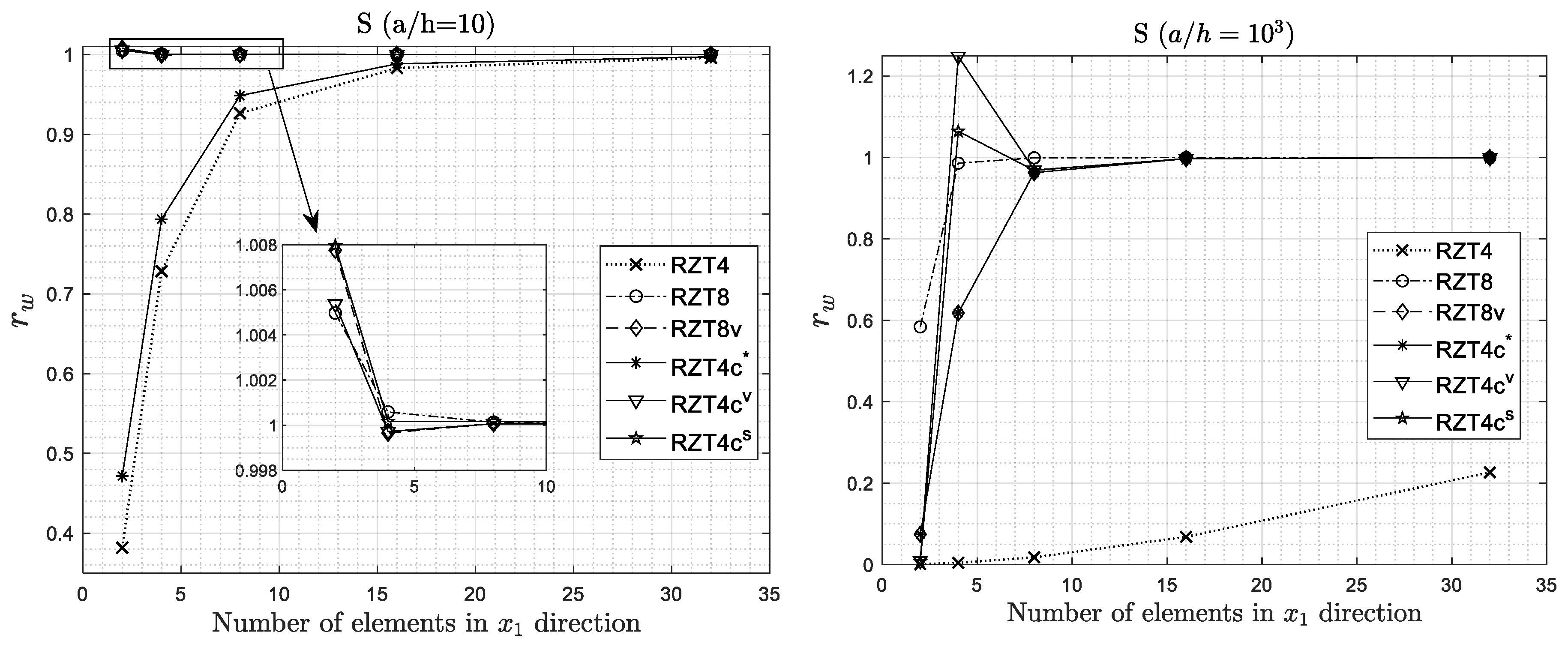
4.2. Convergence Analysis

In this Section, the static convergence characteristic of each element of the family (RZT4, RZT8, RZT8v, and RZT4c) is investigated.
Due to geometry, boundary conditions, and loading symmetry with respect to the reference axes, if not otherwise specified, all FEM results have been obtained meshing only one-quarter of the plate with a regular mesh, i.e., all the elements in the physical plane are square elements (see Section 4.5). Thus, the number of elements indicated below refers to the number of elements along the side of one-quarter of the full-plate.
Thick (a/h = 10) and very thin (a/h = 103) square plates, simply supported on all edges, under uniform pressure of intensity q ¯ 0 , are considered for this analysis: A sandwich plate with thin two-layered cross-ply face-sheet (S), a five-layered cross-ply plate (L), and an isotropic plate (I). The reference (analytical) solutions (Table 4) have been obtained using the Ritz method [69] for the deflection. For the implementation and the convergence analysis of this approximate method, see Reference [69]. In particular, as it is shown in Reference [69], 10 orthogonal polynomials in both x1 and x2 directions are enough to assure the converged Ritz solution. It is clear that when the numerical analyses are performed using the RZT (analytical or with FEM) for the isotropic plate (I), the zigzag terms vanish. Thus, the finite elements formulated on the RZT, for this particular case, coincide with the FSDT ones when the classical shear correction factor is equal to 1 (k2 = 1) and these results are quoted with FSDT4, FSDT8, FSDT8v, and FSDT4c*.
In the RZT4c element, two non-dimensional transverse-shear-parameters ( r L , r T ) appear. For this element, three cases are considered: In the first one, r L and r T are computed as defined by Equation (47) and results are quoted with the label RZT 4 c s ; in the second one, only for the sandwich (S) and laminated (L) plates, we assume the material highly heterogeneous with r L = r T = 1 and results are quoted with the label RZT 4 c v ; in the third one, we assume r L = r T = 0 , such as the isotropic case (I), also for the sandwich (S) and laminate (L) plates and results are quoted with the label RZT 4 c * .
All the FEM results have been obtained using full integration strategy.
Examination of the results plotted in Figure 7, Figure 8 and Figure 9 reveals that the convergence for the most of all elements is monotonic in character, with the exception of the constrained element when used in very thin regime (a/h = 103) and coarse meshes (2 × 2 or 4 × 4). Generally, the convergence rates are different.
Among the four elements, RZT8 is the element with the best convergence rate, followed by RZT8v and RZT4c elements (with different values for non-dimensional transverse-shear-parameters) that are very close to each other and to RZT8 element. On the other hand, RZT8 element has a large number of nodes when compared to the other elements (see Table 5), so its use in the nonlinear static and transient dynamic and failure analyses can result in a very high computational cost, also if meshes with few elements are used. RZT8v has bilinear shape functions for all kinematic variables, with the exception of the deflection, for which quadratic serendipity shape functions are used. Therefore, the number of degrees of freedom is less than the RZT8 element, but higher than RZT4 and RZT4c elements (see Table 5). RZT4c has the same number of nodes as RZT4, but its convergence characteristics are comparable to that RZT8v element. Only the classical four-node RZT4 with bilinear shape functions has a low convergence rate for maximum deflection. Considering the isotropic case (I) the FSDT8v and FSDT4c elements are equivalent in thick and very thin regimes. Except for the RZT4 element, for the 16 × 16 mesh, the error in the FEM results is not higher than 3%. The convergence rates of RZT4c are very similar to the RZT8v, without a great influence of the non-dimensional transverse-shear-parameters ( r L , r T ) . In particular, this element guarantees the same accurate results of the RZT8v with the same dof’s of the RZT4 element. Due to this, the RZT4c element is very interesting from a computational point of view. In Table 5 are reported the total dof’s for each mesh discretization using the various elements: It appears that the RZT4c gives the best compromise between accuracy and low computational cost.
Thus, in the following analyses, if not otherwise specified, an 8 × 8 regular mesh for a quarter of plate is used.

4.3. Effect of Non-Dimensional Transverse Shear Parameters

In the derivation of the RZT4c element from the RZT8v one, there is an element-material dependency by the presence in the element formulation of the two non-dimensional transverse shear parameters r L and r T . In the previous figures (Figure 7, Figure 8 and Figure 9), the effect of these parameters is shown in the convergence results. For the isotropic case, these parameters are no relevant because there is not the zigzag effect. For the cross-ply (L) and sandwich (S) plates, this effect become important in the FEM results. When these parameters are enforced to be r L = r T = 0 , such as the isotropic case, also for the non-homogeneous case, the convergence to the analytical solution is lower than the other cases. This condition is not the best to characterize this element.
Now we consider the RZT 4 c s and RZT 4 c v cases. Table 6 shows the values for r L and r T computed for the cross-ply (L) and the sandwich (S).
The approximation, used for RZT 4 c v cases, is good if we consider the sandwich case, but some differences are present for the cross-ply plate. However, if we consider the results for the cross-ply, there are very few differences between considering r L and r T exactly computed or use r L = r T = 1 . Furthermore, it is preferable not having a material dependency in the element transverse shear strains. This could be a problem if we consider two or more adjacent elements where the material properties are different from one element to another, because at that point there will be two different transverse shear strains.
By taking into consideration these aspects and the good accuracy of the results for the RZT 4 c v case, in the remaining part of the paper, the RZT4c element is used only considering the case r L = r T = 1 .

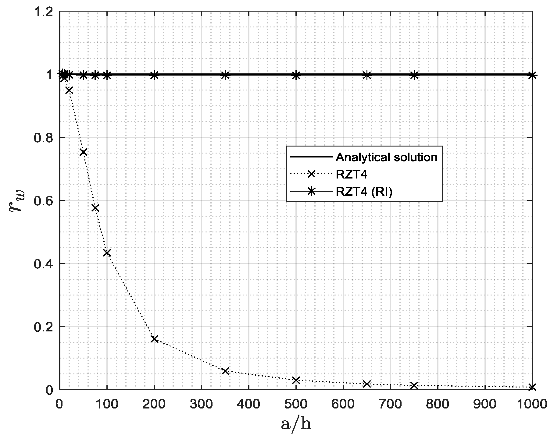
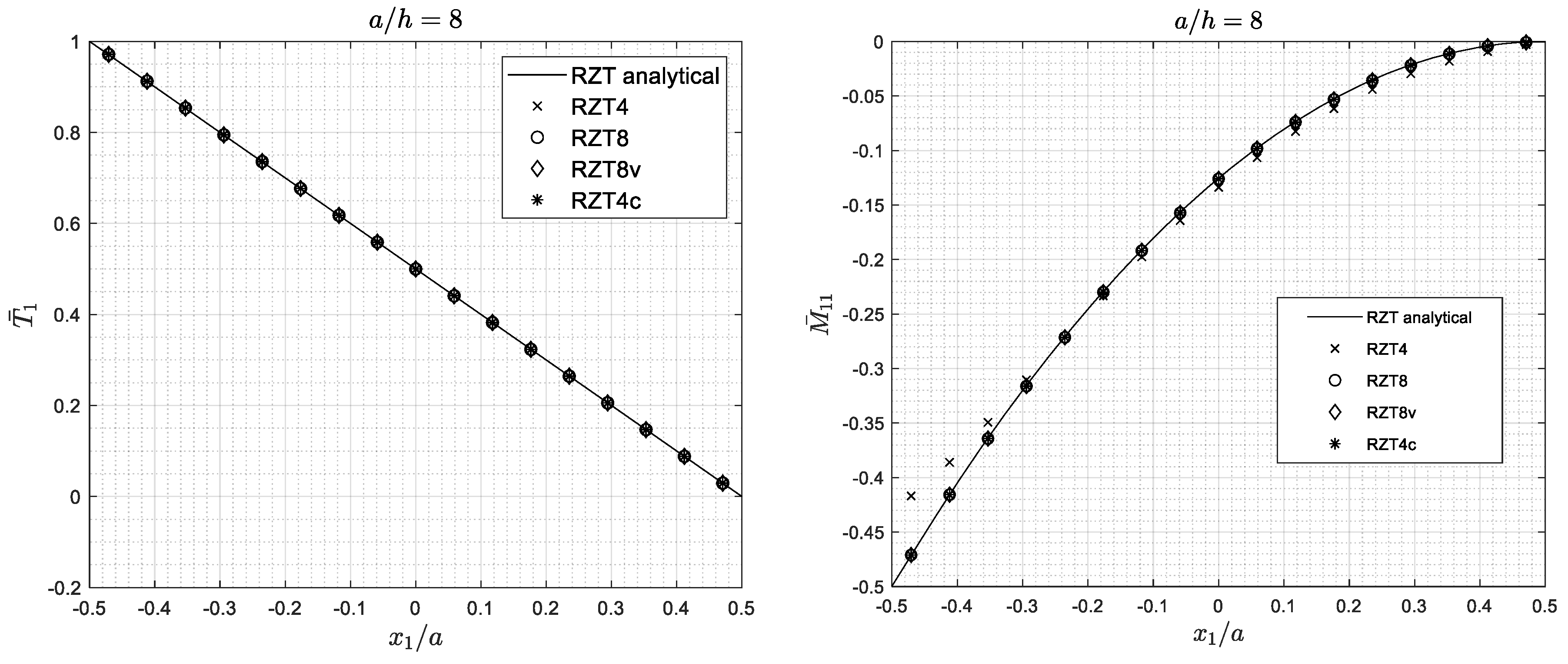
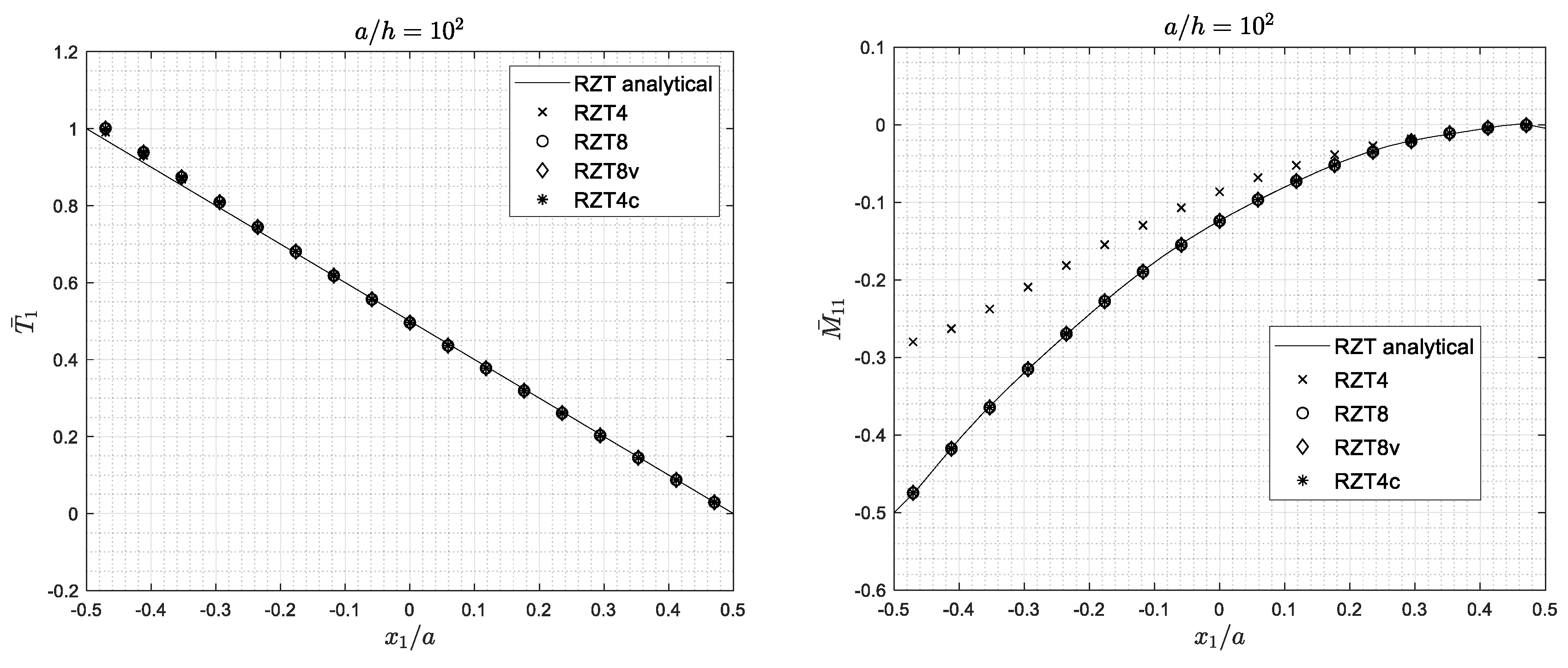
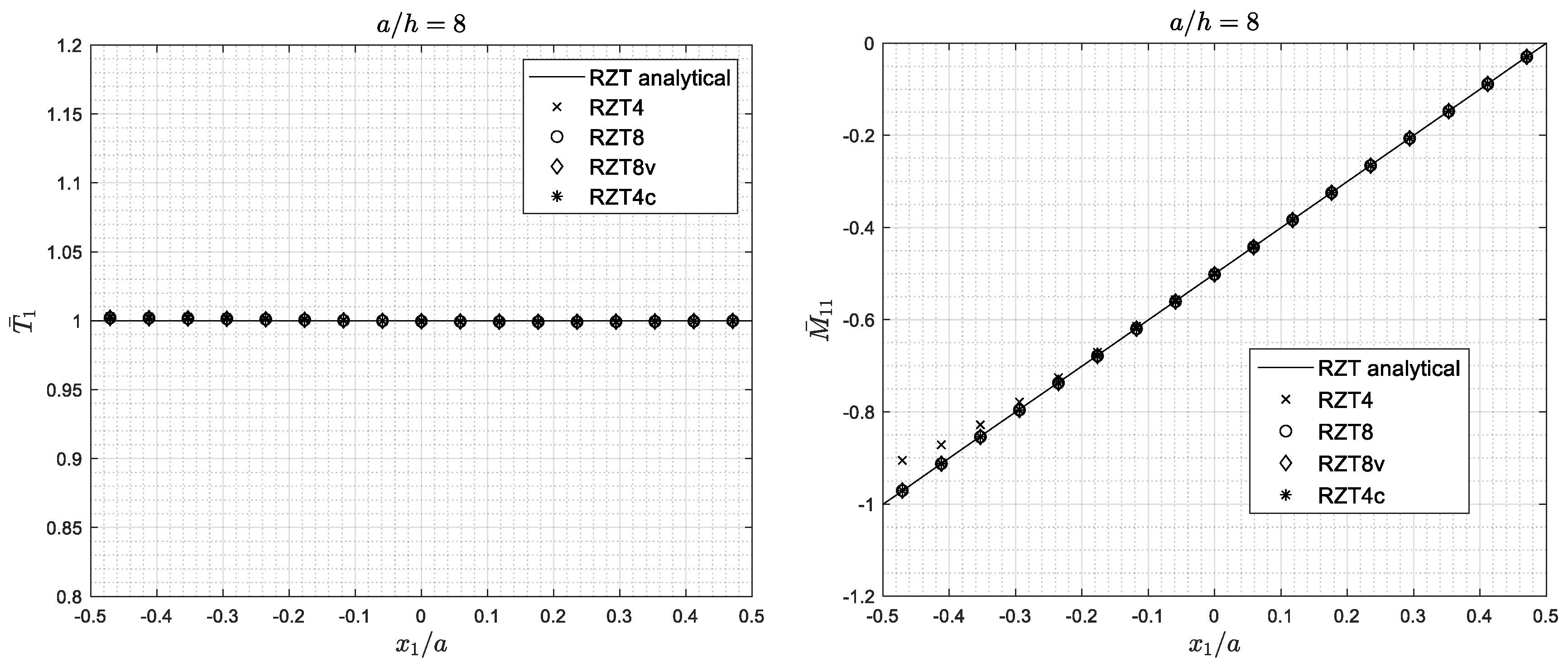
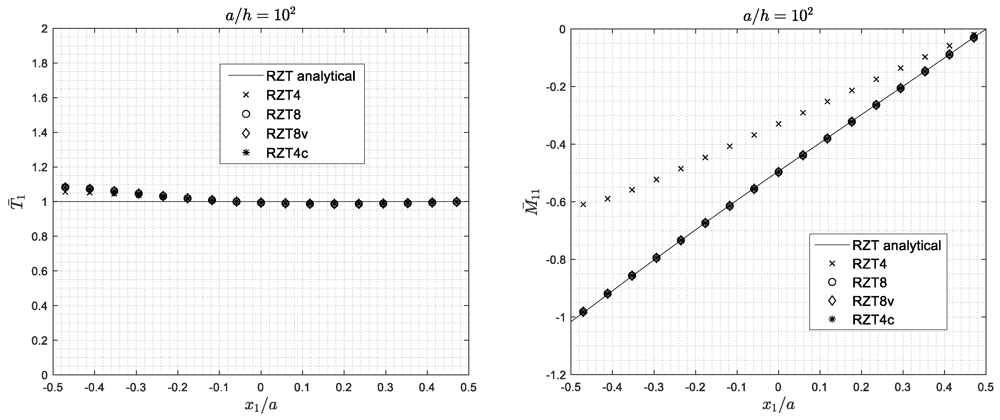
4.4. Shear Locking Phenomenon

In order to assess the behaviour of the four plate elements with respect to the shear-locking effect, Figure 10 shows results for the maximum deflection (rw) ratio as a function of the span-to-thickness ratio, a/h, for a simply supported five-layered symmetric cross-ply plate (L) under bi-sinusoidal transverse pressure, considering a 4 × 4 and an 8 × 8 mesh. The results quoted as RZT4 refer to the 4-node quadrilateral element using full integration.
As is well known, the shear-locking effect is pathological for the full integrated RZT4 element—as is well known, the use of stabilisation techniques could avoid the appearance of hourglass modes; other code-specific techniques that have been also proposed (typically based on EAS or ANS), do not introduce any spurious mode, for both 4 × 4 and 8 × 8 mesh patterns. RZT4 is suitable only for the analysis of thick and moderately thick plates. RZT8 shows very good performances over a very large range of span-to-thickness ratios (from 6 to 103), with some initial effects of transverse shear locking appearing for very thin plate (a/h = 103). A good compromise between the accuracy of the RZT8 and the computational efficiency of the classical four node appears to be RZT8v. RZT4c perform very similar to RZT8v, but with a lower computational cost, equal to that of RZT4 element.
As we said, in the literature and in the FEM commercial codes, the shear locking effect is typically addressed using the reduced integration technique when computing the shear terms in the stiffness matrix.
Figure 11 shows the behaviour of the RTZ4 element using full and reduced integration. It is easily concluded that the reduced integration strategy improves the performances of RTZ4. Yet, one typical problem affecting the reduced integration technique is the singularity of the stiffness matrix for very thin plate. This leads to the appearance of extra zero strain energy modes (called spurious mode), the so-called hourglass effect.
Table 7 gives the number of rigid body modes for the various plate elements. As expected, we have three rigid translations along the axes and three rigid rotation around the axes for all the elements, with the exception of the RZT4 with reduced integration, where an extra zero-energy mode (spurious mode) appears. The other elements, RZT8, RZT8v, and RZT4c, are free from this unlikely effect.
In the remaining part of the paper, the full integration is used for all the C0 family elements.

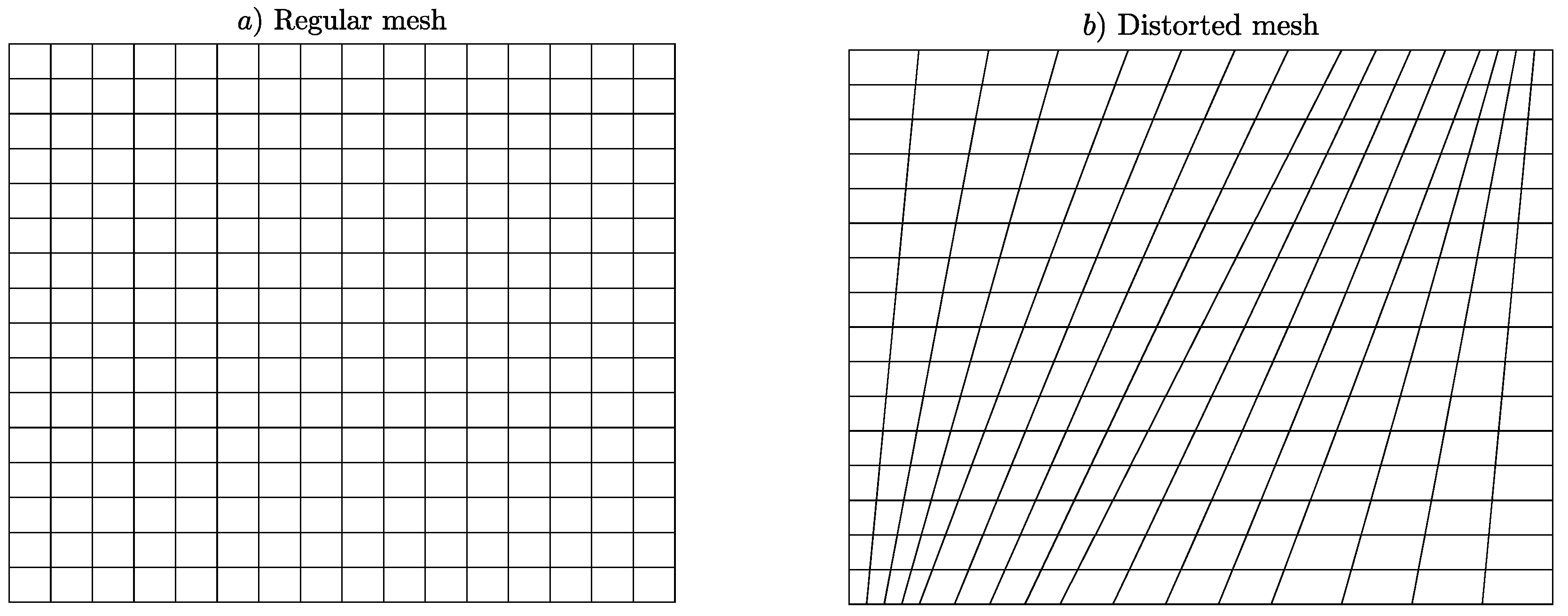
4.5. Distorted and Regular Mesh Analysis

As is well known, the performances of the plate finite elements depend also on their skewness ratio, i.e., on the degree of the distortion of their plan form geometry. Figure 12a,b respectively gives the regular and distorted 16 × 16 mesh for the whole plate used in this study.
To assess the relative performances of the RZT elements when used in distorted geometry, a cantilever square sandwich plate (S) and multi-layered cross-ply plate (L) are investigated. Thick (a/h = 8) and very thin (a/h = 103) plates are considered.
Table 8 gives the percent errors of FEM results on the maximum non-dimensional deflection under three types of load distribution (in Figure 13 are shown: Uniform distribution, constant uniform edge load, and two vertical opposite tip forces), using regular and distorted 16 × 16 meshes. For simplicity, the load cases are named as follows: C1 for the uniform transverse load pressure, C2 for the constant uniform edge load, and C3 for the two vertical opposite tip forces. For the same plates and meshes, Table 9 gives the percent errors of FEM results on the undamped fundamental frequency parameter. The percent error is defined as
e r r % = ( F E M A N A L Y T I C A L 1 ) 100 %
The analytical solutions have been obtained using the Ritz method [69]. In particular, as it is shown in Reference [69], 10 orthogonal polynomials in both x1 and x2 directions are enough to assure the converged Ritz solution.
As expected, regular meshes give results closer to the analytical ones. As before, RZT8 has the best performances also for distorted meshes, but at expense of higher computational costs. Again, RTZ4c appears to be a good compromise between accuracy and computational cost.
To further assess the performance of the RZT elements, the bending behaviour of a sandwich (S) cantilevered plates is investigated, comparing the bending moment and the transverse shear force distributions along the midline of the plate with the analytical ones. Two square plates (S) are considered, both loaded with the load distribution C1 (uniform transverse load) and C2 (uniform constant edge load) and meshed with 17 × 17 elements: (i) A thick plate (a/h = 8; a/b = 1) and (ii) a thin plate (a/h = 102; a/b = 1). The analytical solutions have been obtained using the Ritz method [69] with 10 orthogonal functions in x1 direction and 10 orthogonal functions in x2 direction. Plots of the distributions of shear force and bending moment along the midline of the plates parallel to x1 axis are given in Figure 14 (thick sandwich plate) and Figure 15 (thin sandwich plate) for the C1 load condition and in Figure 16 (thick sandwich plate) and Figure 17 (thin sandwich plate) for the C2 load condition. The shear force and bending moment were computed using the finite element correspond to the centroid of each elements on the midline of the plate. The shear force and bending moment are normalized as follows for the C1 load condition:
T ¯ 1 = T 1 q ¯ 0 a ; M ¯ 11 = M 11 q ¯ 0 a 2
and for the C2 load condition as follows:
T ¯ 1 = T 1 T ¯ 13 ; M ¯ 11 = M 11 T ¯ 13 a .
Also, in this test, RZT4c element shows its good accuracy in estimating the shear force also near the clamped edge for thick sandwich plates.

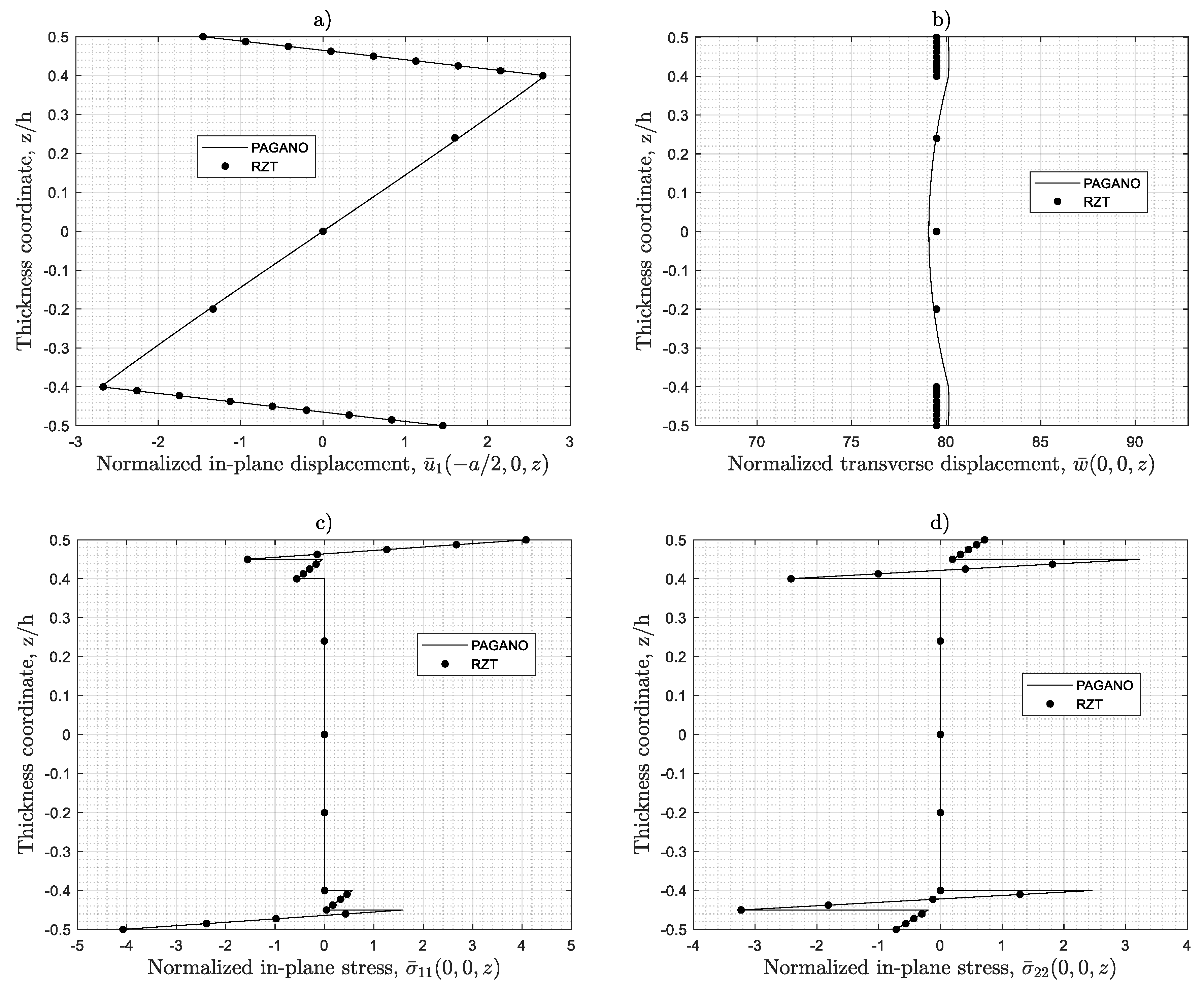
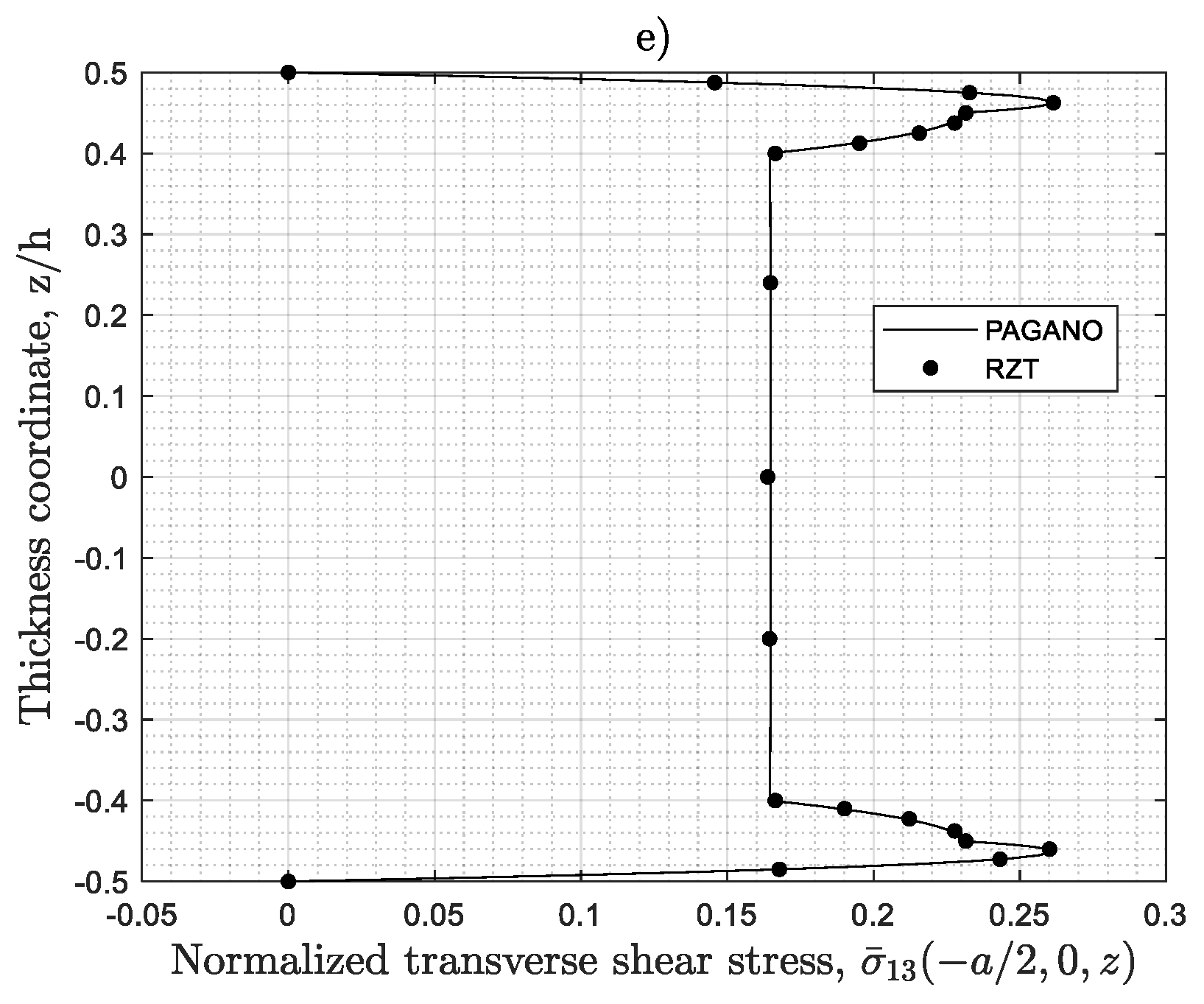
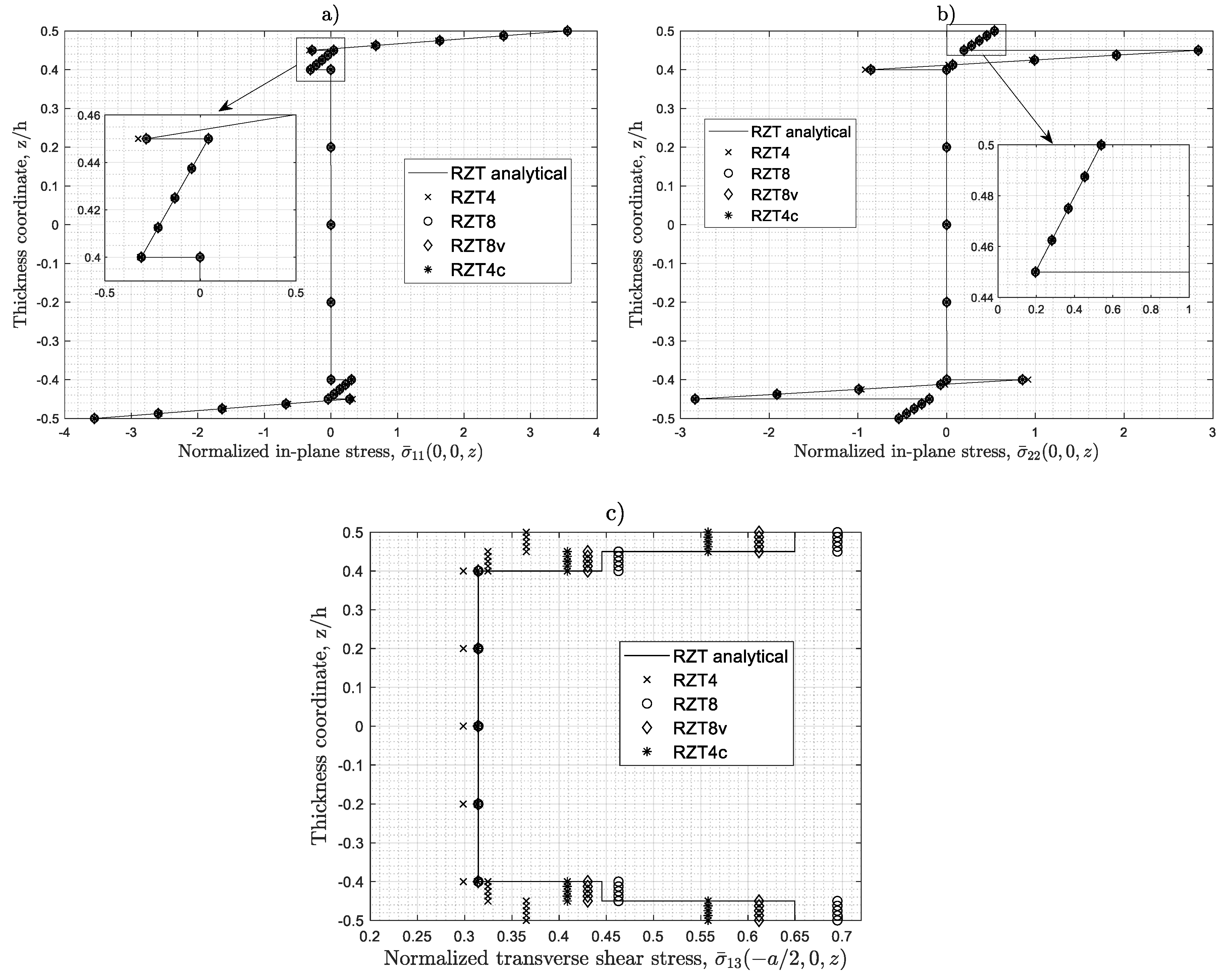
4.6. Stress Distributions

In order to show the ability of FEM solutions to capture also the local behaviour (distribution of the stresses along the thickness), we consider bending under transverse uniform pressure of simply supported sandwich plate (S) for a/h = 8.
Figure 18 compares the distributions of in-plane stresses at the centre of the plates and the transverse shear stress at the midpoint of the left edge, computed using the Ritz method [69] and the family of C0 RZT plate elements. For this study, in order to have a better distribution of the stresses, a regular mesh 16 × 16 for a quarter of plate has been adopted.
These results confirm in general the good accuracy of these elements to estimate the thickness-wise distributions of the in-plane stresses, while some difference when the transverse shear stresses are considered. As expected, for both sandwich (S), the RZT8 shows the best performances, followed by the RZT8v and the RZT4c. By taking into account that RTZ8 is computationally more expensive and that RTZ4 with reduced integration is penalized by the zero energy strain modes, it can be concluded that RZT4c represents the best compromise between accuracy and computational costs.

5. Concluding Remarks

A family of four C0 quadrilateral plate elements based on the refined zigzag theory has been developed and numerically tested.
The numerical assessment given in the previous Section reveals that:
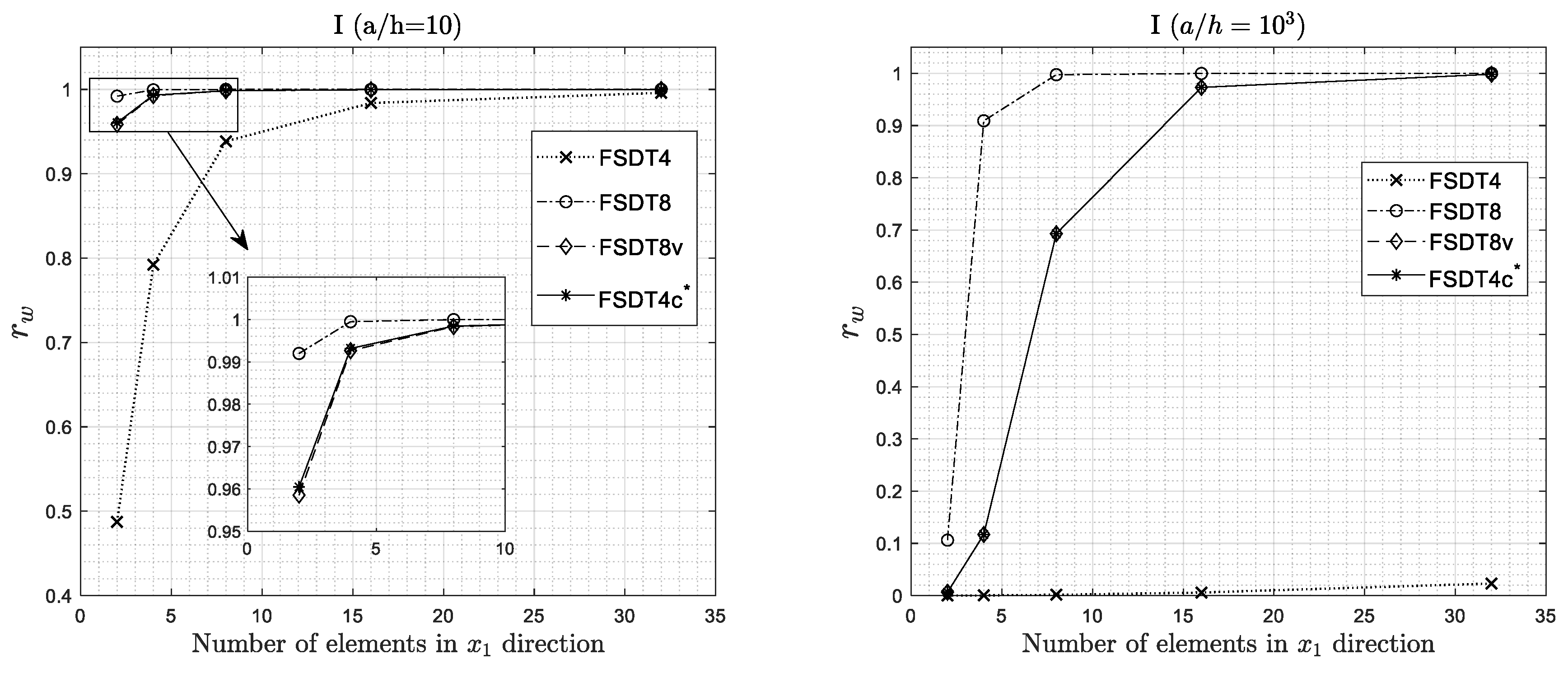
  • The convergence of the FEM solution for all the elements of the family is in general monotonic in character, although with different rates.
  • The bi-linear 4-node element (RZT4) is strongly affected by the shear locking effect in thin plates when full integration is used.
  • The bi-linear 4-node element (RZT4) has performances comparable to the other elements in the range of thin plates when reduced integration (RI) is adopted, but presents extra zero strain energy modes, if no stabilization technique is used.
  • The serendipity 8-node element (RZT8), the virgin 8-node element (RZT8v), and the 4-node anisoparametric constrained element (RZT4c) show good performance and predictive capabilities for various problems, and the transverse shear-locking is greatly relieved without using any reduced integration schemes, for thin plate (aspect ratio equal to 5 × 10²) at least for mesh 8 × 8.
  • All elements, except for the conventional bi-linear RZT4 element with full integration, are adequate to predict the bending global response (transverse displacement, distribution of the transverse shear resultant, and bending moment) and undamped frequencies. The same holds for the predictive capabilities of the local behaviour (thickness-wise distributions of the bending stresses and transverse shear stresses).
  • RZT4c has well-conditioned element stiffness matrix, contrary to RZT4 when reduced integration strategy is used.
  • The computational cost of RTZ4c is much lower than that of RTZ8 and RTZ8v elements.
  • The accuracy of all the elements is sensitive to their degree of planform distortion.
Therefore, due its good numerical accuracy (generally comparable to that of RZT8 and RZT8v elements) and low computational cost (equal to that of RZT4 element), RTZ4c quadrilateral plate element appears to be a good candidate for the FEM analysis of laminated composite and sandwich plates, mainly when nonlinear or transient linear and nonlinear analyses are involved. As a general concluding remark, the presented results show clearly that RZT8 is the most robust element among those considered in the present investigation. Moreover, as it is well known, the quadrilateral isoparametric 8-node FE is not an optimal element. The final conclusion is that further studies based on different approaches should be carried out to propose a locking-free RZT plate FE. Therefore, following Tessler and Hughes [60,62] suggestions, in a work in progress, the concept of an appropriate element shear correction factor is adopted in conjunction with the anisotropic constrained strategy to further alleviate the shear locking effect (extend the range of the plate aspect ratios until 106).

Author Contributions

Conceptualization, M.D.S. and M.S.; methodology, M.D.S.; software, M.S.; validation, M.D.S. and M.S.; formal analysis, M.D.S. and M.S.; investigation, M.D.S. and M.S.; resources, M.D.S. and M.S.; data curation, M.D.S. and M.S.; writing—original draft preparation, M.D.S. and M.S.; writing—review and editing, M.D.S. and M.S.; visualization, M.D.S. and M.S.; supervision, M.D.S.; project administration, M.D.S.

Funding

This research received no external funding.

Acknowledgments

The authors acknowledge the helpful discussion with Alexander Tessler, distinguished Researcher at NASA LRC Hampton VA, during its period as Visiting Professor at Politecnico di Torino, Italy, Department of Mechanical and Aerospace Engineering.

Conflicts of Interest

The authors declare no conflict of interest.

References

  1. Abrate, S.; di Sciuva, M. Equivalent single layer theories for composite and sandwich structures: A review. Compos. Struct. 2017, 179, 482–494. [Google Scholar] [CrossRef]
  2. Abrate, S.; di Sciuva, M. Multilayer models for composite and sandwich structures. In Comprehensive Composite Materials II; Beaumont, P.W.R., Zweben, C.H., Eds.; Elsevier: Amsterdam, The Netherlands, 2018; pp. 399–425. ISBN 978-0-08-100534-7. [Google Scholar]
  3. Whitney, J.M.; Pagano, N.J. Shear deformation in heterogeneous anisotropic plates. J. Appl. Mech. 1970, 37, 1031–1036. [Google Scholar] [CrossRef]
  4. Reddy, J.N. Mechanics of Laminated Composite Plates and Shells: Theory and Analysis, 2nd ed.; CRC Press: Boca Raton, FL, USA, 2003; ISBN 978-0-203-50280-8. [Google Scholar]
  5. Pandya, B.N.; Kant, T. Finite element analysis of laminated composite plates using a higher-order displacement model. Compos. Sci. Technol. 1988, 32, 137–155. [Google Scholar] [CrossRef]
  6. Zhang, Y.X.; Yang, C.H. Recent developments in finite element analysis for laminated composite plates. Compos. Struct. 2009, 88, 147–157. [Google Scholar] [CrossRef]
  7. Dau, F.; Polit, O.; Touratier, M. An efficient C1 finite element with continuity requirements for multilayered/sandwich shell structures. Comput. Struct. 2004, 82, 1889–1899. [Google Scholar] [CrossRef]
  8. Dau, F.; Polit, O.; Touratier, M. C1 plate and shell finite elements for geometrically nonlinear analysis of multilayered structures. Comput. Struct. 2006, 84, 1264–1274. [Google Scholar] [CrossRef]
  9. Polit, O.; Vidal, P.; D’Ottavio, M. Robust C0 high-order plate finite element for thin to very thick structures: Mechanical and thermo-mechanical analysis. Int. J. Numer. Methods Eng. 2012, 90, 429–451. [Google Scholar] [CrossRef]
  10. Reddy, J.N. A generalization of two-dimensional theories of laminated composite plates. Commun. Appl. Numer. Methods 1987, 3, 173–180. [Google Scholar] [CrossRef]
  11. Reddy, J.N. An evaluation of equivalent-single-layer and layerwise theories of composite laminates. Compos. Struct. 1993, 25, 21–35. [Google Scholar] [CrossRef]
  12. Guo, Y.; Nagy, A.P.; Gürdal, Z. A layerwise theory for laminated composites in the framework of isogeometric analysis. Compos. Struct. 2014, 107, 447–457. [Google Scholar] [CrossRef]
  13. Liu, B.; Ferreira, A.J.M.; Xing, Y.F.; Neves, A.M.A. Analysis of composite plates using a layerwise theory and a differential quadrature finite element method. Compos. Struct. 2016, 156, 393–398. [Google Scholar] [CrossRef]
  14. Di Sciuva, M. Bending, vibration and buckling of simply supported thick multilayered orthotropic plates: An evaluation of a new displacement model. J. Sound Vib. 1986, 105, 425–442. [Google Scholar] [CrossRef]
  15. Di Sciuva, M. An improved shear-deformation theory for moderately thick multilayered anisotropic shells and plates. J. Appl. Mech. 1987, 54, 589–596. [Google Scholar] [CrossRef]
  16. Di Sciuva, M. Multilayered anisotropic plate models with continuous interlaminar stresses. Compos. Struct. 1992, 22, 149–167. [Google Scholar] [CrossRef]
  17. Di Sciuva, M. Development of an anisotropic, multilayered, shear-deformable rectangular plate element. Comput. Struct. 1985, 21, 789–796. [Google Scholar] [CrossRef]
  18. Di Sciuva, M. Evaluation of some multilayered, shear-deformable plate elements. Comput. Struct. 1986, 24, 845–854. [Google Scholar] [CrossRef]
  19. Di Sciuva, M. A general quadrilateral multilayered plate element with continuous interlaminar stresses. Comput. Struct. 1993, 47, 91–105. [Google Scholar] [CrossRef]
  20. Di Sciuva, M. A third-order triangular multilayered plate finite element with continuous interlaminar stresses. Int. J. Numer. Methods Eng. 1995, 38, 1–26. [Google Scholar] [CrossRef]
  21. Tessler, A.; di Sciuva, M.; Gherlone, M. Refinement of Timoshenko Beam Theory for Composite and Sandwich Beams Using Zigzag Kinematics; NASA/TP-2007-215086; NASA Langley Research Center: Hampton, VA, USA, 2007; pp. 1–45.
  22. Tessler, A.; di Sciuva, M.; Gherlone, M. Refined Zigzag Theory for Laminated Composite and Sandwich Plates; NASA/TP-2009-215561; NASA Langley Research Center: Hampton, VA, USA, 2009; pp. 1–53.
  23. Tessler, A.; di Sciuva, M.; Gherlone, M. A refined zigzag beam theory for composite and sandwich beams. J. Compos. Mater. 2009, 43, 1051–1081. [Google Scholar] [CrossRef]
  24. Iurlaro, L.; Gherlone, M.; di Sciuva, M.; Tessler, A. Assessment of the refined zigzag theory for bending, vibration, and buckling of sandwich plates: A comparative study of different theories. Compos. Struct. 2013, 106, 777–792. [Google Scholar] [CrossRef]
  25. Gherlone, M. On the use of zigzag functions in equivalent single layer theories for laminated composite and sandwich beams: A comparative study and some observations on external weak layers. J. Appl. Mech. 2013, 80, 061004. [Google Scholar] [CrossRef]
  26. Gherlone, M.; Tessler, A.; di Sciuva, M. C0 beam elements based on the refined zigzag theory for multilayered composite and sandwich laminates. Compos. Struct. 2011, 93, 2882–2894. [Google Scholar] [CrossRef]
  27. Oñate, E.; Eijo, A.; Oller, S. Simple and accurate two-noded beam element for composite laminated beams using a refined zigzag theory. Comput. Methods Appl. Mech. Eng. 2012, 213–216, 362–382. [Google Scholar] [CrossRef]
  28. Versino, D.; Gherlone, M.; Mattone, M.C.; di Sciuva, M.; Tessler, A. C0 triangular elements based on the refined zigzag theory for multilayered composite and sandwich plates. Compos. Part B Eng. 2013, 44, 218–230. [Google Scholar] [CrossRef]
  29. Eijo, A.; Oñate, E.; Oller, S. A four-noded quadrilateral element for composite laminated plates/shells using the refined zigzag theory. Int. J. Numer. Methods Eng. 2013, 95, 631–660. [Google Scholar] [CrossRef]
  30. Eijo, A.; Oñate, E.; Oller, S. A numerical model of delamination in composite laminated beams using the LRZ beam element based on the refined zigzag theory. Compos. Struct. 2013, 104, 270–280. [Google Scholar] [CrossRef]
  31. Eijo, A.; Oñate, E.; Oller, S. Delamination in laminated plates using the 4-noded quadrilateral QLRZ plate element based on the refined zigzag theory. Compos. Struct. 2014, 108, 456–471. [Google Scholar] [CrossRef]
  32. Versino, D.; Gherlone, M.; di Sciuva, M. Four-node shell element for doubly curved multilayered composites based on the refined zigzag theory. Compos. Struct. 2014, 118, 392–402. [Google Scholar] [CrossRef]
  33. Treviso, A.; Mundo, D.; Tournour, M. A C0-continuous RZT beam element for the damped response of laminated structures. Compos. Struct. 2015, 131, 987–994. [Google Scholar] [CrossRef]
  34. Di Sciuva, M.; Gherlone, M.; Iurlaro, L.; Tessler, A. A class of higher-order C0 composite and sandwich beam elements based on the refined zigzag theory. Compos. Struct. 2015, 132, 784–803. [Google Scholar] [CrossRef]
  35. Groh, R.M.J.; Weaver, P.M. On displacement-based and mixed-variational equivalent single layer theories for modelling highly heterogeneous laminated beams. Int. J. Solids Struct. 2015, 59, 147–170. [Google Scholar] [CrossRef] [Green Version]
  36. Iurlaro, L. Development of Refined Models for Multilayered Composite and Sandwich Structures: Analytical Formulation, FEM Implementation and Experimental Assessment. Ph.D. Thesis, Politecnico di Torino, Torino, Italy, 2015. [Google Scholar]
  37. Treviso, A.; Mundo, D.; Tournour, M. Dynamic response of laminated structures using a refined zigzag theory shell element. Compos. Struct. 2017, 159, 197–205. [Google Scholar] [CrossRef]
  38. Oñate, E. Structural Analysis with the Finite Element Method. Linear Statics: Volume 2: Beams, Plates and Shells; Lecture Notes on Numerical Methods in Engineering and Sciences; Springer: Dordrecht, The Netherlands, 2013; ISBN 978-1-4020-8742-4. [Google Scholar]
  39. Babuška, I.; Suri, M. Locking effects in the finite element approximation of elasticity problems. Numer. Math. 1992, 62, 439–463. [Google Scholar] [CrossRef]
  40. Babuška, I.; Suri, M. On locking and robustness in the finite element method. SIAM J. Numer. Anal. 1992, 29, 1261–1293. [Google Scholar] [CrossRef]
  41. Barut, A.; Madenci, E.; Tessler, A. Nonlinear analysis of laminates through a mindlin-type shear deformable shallow shell element. Comput. Methods Appl. Mech. Eng. 1997, 143, 155–173. [Google Scholar] [CrossRef]
  42. Barut, A.; Madenci, E.; Tessler, A. Nonlinear thermoelastic analysis of composite panels under non-uniform temperature distribution. Int. J. Solids Struct. 2000, 37, 3681–3713. [Google Scholar] [CrossRef]
  43. Zienkiewicz, O.C.; Taylor, R.L.; Too, J.M. Reduced integration technique in general analysis of plates and shells. Int. J. Numer. Methods Eng. 1971, 3, 275–290. [Google Scholar] [CrossRef]
  44. Hughes, T.J.R.; Taylor, R.L.; Kanoknukulchai, W. A simple and efficient finite element for plate bending. Int. J. Numer. Methods Eng. 1977, 11, 1529–1543. [Google Scholar] [CrossRef]
  45. Pugh, E.D.L.; Hinton, E.; Zienkiewicz, O.C. A study of quadrilateral plate bending elements with ‘reduced’ integration. Int. J. Numer. Methods Eng. 1978, 12, 1059–1079. [Google Scholar] [CrossRef]
  46. Hughes, T.J.R.; Cohen, M.; Haroun, M. Reduced and selective integration techniques in the finite element analysis of plates. Nucl. Eng. Des. 1978, 46, 203–222. [Google Scholar] [CrossRef]
  47. Stricklin, J.A.; Haisler, W.E.; Tisdale, P.R.; Gunderson, R. A rapidly converging triangular plate element. AIAA J. 1969, 7, 180–181. [Google Scholar] [CrossRef]
  48. Batoz, J.-L.; Bathe, K.-J.; Ho, L.-W. A study of three-node triangular plate bending elements. Int. J. Numer. Methods Eng. 1980, 15, 1771–1812. [Google Scholar] [CrossRef]
  49. Dvorkin, E.N.; Bathe, K. A continuum mechanics based four-node shell element for general non-linear analysis. Eng. Comput. 1984, 1, 77–88. [Google Scholar] [CrossRef] [Green Version]
  50. Ko, Y.; Lee, P.-S.; Bathe, K.-J. A new MITC4+ shell element. Comput. Struct. 2017, 182, 404–418. [Google Scholar] [CrossRef]
  51. Hughes, T.J.R. Equivalence of finite elements for nearly incompressible elasticity. J. Appl. Mech. 1977, 44, 181–183. [Google Scholar] [CrossRef] [Green Version]
  52. De Souza Neto, E.A.; Perić, D.; Dutko, M.; Owen, D.R.J. Design of simple low order finite elements for large strain analysis of nearly incompressible solids. Int. J. Solids Struct. 1996, 33, 3277–3296. [Google Scholar] [CrossRef]
  53. De Souza Neto, E.A.; Pires, F.M.A.; Owen, D.R.J. F-bar-based linear triangles and tetrahedra for finite strain analysis of nearly incompressible solids. Part I: Formulation and benchmarking. Int. J. Numer. Methods Eng. 2005, 62, 353–383. [Google Scholar] [CrossRef]
  54. Hughes, T.J.R.; Tezduyar, T.E. Finite elements based upon mindlin plate theory with particular reference to the four-node bilinear isoparametric element. J. Appl. Mech. 1981, 48, 587–596. [Google Scholar] [CrossRef]
  55. Katili, I. A new discrete Kirchhoff-Mindlin element based on Mindlin-Reissner plate theory and assumed shear strain fields—Part I: An extended DKT element for thick-plate bending analysis. Int. J. Numer. Methods Eng. 1993, 36, 1859–1883. [Google Scholar] [CrossRef]
  56. Katili, I. A new discrete Kirchhoff-Mindlin element based on Mindlin–Reissner plate theory and assumed shear strain fields—Part II: An extended DKQ element for thick-plate bending analysis. Int. J. Numer. Methods Eng. 1993, 36, 1885–1908. [Google Scholar] [CrossRef]
  57. Bletzinger, K.-U.; Bischoff, M.; Ramm, E. A unified approach for shear-locking-free triangular and rectangular shell finite elements. Comput. Struct. 2000, 75, 321–334. [Google Scholar] [CrossRef]
  58. Tessler, A.; Dong, S.B. On a hierarchy of conforming Timoshenko beam elements. Comput. Struct. 1981, 14, 335–344. [Google Scholar] [CrossRef]
  59. Tessler, A. Comparison of interdependent interpolation for membrane and bending kinematics in shear-deformable shell elements. In Proceedings of the Eight International Conference on Computational Engineering and Science, Anaheim, CA, USA, 18–24 August 2000; p. 7. [Google Scholar]
  60. Tessler, A.; Hughes, T.J.R. An improved treatment of transverse shear in the mindlin-type four-node quadrilateral element. Comput. Methods Appl. Mech. Eng. 1983, 39, 311–335. [Google Scholar] [CrossRef]
  61. Tessler, A. A priori identification of shear locking and stiffening in triangular mindlin elements. Comput. Methods Appl. Mech. Eng. 1985, 53, 183–200. [Google Scholar] [CrossRef]
  62. Tessler, A.; Hughes, T.J.R. A three-node Mindlin plate element with improved transverse shear. Comput. Methods Appl. Mech. Eng. 1985, 50, 71–101. [Google Scholar] [CrossRef]
  63. Tessler, A. Shear-deformable, anisoparametric flexure elements with penalty relaxation. In Finite Element Methods for Plate and Shell Structures; Pineridge Press: London, UK, 1986. [Google Scholar]
  64. Fried, I.; Johnson, A.; Tessler, A. Minimal-degree thin triangular plate and shell bending finite elements of order two and four. Comput. Methods Appl. Mech. Eng. 1986, 56, 283–307. [Google Scholar] [CrossRef]
  65. Tessler, A.; Spiridigliozzi, L. Resolving membrane and shear locking phenomena in curved shear-deformable axisymmetric shell elements. Int. J. Numer. Methods Eng. 1988, 26, 1071–1086. [Google Scholar] [CrossRef]
  66. Tessler, A. A C0-anisoparametric three-node shallow shell element. Comput. Methods Appl. Mech. Eng. 1990, 78, 89–103. [Google Scholar] [CrossRef]
  67. Tessler, A. An efficient, conforming axisymmetric shell element including transverse shear and rotary inertia. Comput. Struct. 1982, 15, 567–574. [Google Scholar] [CrossRef]
  68. Pagano, N.J. Exact solutions for rectangular bidirectional composites and sandwich plates. J. Compos. Mater. 1970, 4, 20–34. [Google Scholar] [CrossRef]
  69. Di Sciuva, M.; Sorrenti, M. Bending and free vibration analysis of functionally graded sandwich plates: An assessment of the refined zigzag theory. J. Sandw. Struct. Mater. 2019, 16, 669–699. [Google Scholar] [CrossRef]
Figure 1. Multilayer plate: Geometry and reference frame.
Jcs 03 00100 g001
Figure 2. Contributions to the in plane refined zigzag theory (RZT) kinematics for a three-layered laminate.
Jcs 03 00100 g002
Figure 3. Eight-node quadrilateral plate element in the physical plane (a) and natural plane (b).
Jcs 03 00100 g003
Figure 4. Eight-node virgin quadrilateral plate element. Geometry, physical co-ordinates (x1, x2), and natural co-ordinates (ξ, η). Boundary co-ordinate system (n, s). Definition of the parameters aij and bij entering in Equations (56) and (63) and the positive rotations (θ1, θ2) and (θn, θs).
Jcs 03 00100 g004
Figure 5. Nodal dof’s (transverse deflection, bending rotations, and zigzag amplitudes) and edge co-ordinate, s.
Jcs 03 00100 g005
Figure 6. Bending of a square sandwich plate (S), simply supported on all edges under transverse sinusoidal pressure (span-to-thickness ratio, a/h = 6). (a) Normalized in-plane displacement ( u ¯ 1 ) ; (b) Normalized transverse displacement ( w ¯ ) ; (c) Normalized in-plane stress ( σ ¯ 11 ) ; (d) Normalized in-plane stress ( σ ¯ 22 ) ; (e) Normalized transverse shear stress ( σ ¯ 13 ) .
Jcs 03 00100 g006aJcs 03 00100 g006b
Figure 7. Convergence analysis of the Finite Element Method (FEM) solution for the isotropic plate (I). Regular mesh.
Jcs 03 00100 g007
Figure 8. Convergence analysis of the FEM solution for the laminated plate (L). Regular mesh.
Jcs 03 00100 g008
Figure 9. Convergence analysis of the FEM solution for the sandwich plate (S). Regular mesh.
Jcs 03 00100 g009
Figure 10. Shear-locking effect analysis. Laminate L, (a) mesh 4 × 4, and (b) mesh 8 × 8 of a quarter of the plate.
Jcs 03 00100 g010
Figure 11. Shear-locking effect analysis for RZT4 element using full and reduced integration. Laminate L. Mesh 8 × 8 of a quarter of the plate.
Jcs 03 00100 g011
Figure 12. Regular (a) and distorted (b) 16 × 16 mesh.
Jcs 03 00100 g012
Figure 13. Load distributions for cantilever plates: (a) Uniform pressure (C1), (b) uniform pressure along the free edge (C2), (c) two opposite vertical forces (C3).
Jcs 03 00100 g013
Figure 14. Cantilever thick sandwich (S) square plate under uniform transverse pressure (C1). Transverse shear force and bending moment distribution.
Jcs 03 00100 g014
Figure 15. Cantilever thin sandwich (S) square plate under uniform transverse pressure (C1). Transverse shear force and bending moment distribution.
Jcs 03 00100 g015
Figure 16. Cantilever thick sandwich (S) square plate under uniform edge transverse pressure (C2). Transverse shear force and bending moment distribution.
Jcs 03 00100 g016
Figure 17. Cantilever thin sandwich (S) square plate under uniform edge transverse pressure (C2). Transverse shear force and bending moment distribution.
Jcs 03 00100 g017
Figure 18. Non-dimensional bending and transverse shear stresses. Simply supported sandwich (S) square plate under uniform transverse pressure (a/h = 8). (a) Normalized in-plane stress ( σ ¯ 11 ) ; (b) Normalized in-plane stress ( σ ¯ 22 ) ; (c) Normalized transverse shear stress ( σ ¯ 13 ) .
Jcs 03 00100 g018
Table 1. The family of C0 quadrilateral plate elements formulated and assessed in this study. Acronyms, topology, degrees of freedom (dof’s), and shape functions.
Element TypeNodal ConfigurationDegrees of FreedomShape FunctionsNote
RZT4 Jcs 03 00100 i00128 N i ( ξ , η ) = L i ( ξ , η ) ( i = 1 ÷ 4 ) -
RZT8 Jcs 03 00100 i00256 N i w ( ξ , η ) = P i ( ξ , η )   ( i = 1 ÷ 8 ) -
RZT8v Jcs 03 00100 i00332 ( N d ) i ( ξ , η ) = L i ( ξ , η )   ( i = 1 ÷ 4 ) ( d u x , u y , θ x , θ y , ψ x , ψ x )
N i w ( ξ , η ) = P i ( ξ , η )   ( i = 1 ÷ 8 )
-
RZT4c Jcs 03 00100 i00428 ( N d ) i ( ξ , η ) = L i ( ξ , η )   ( i = 1 ÷ 4 ) ( d u 1 , u 2 , θ 1 , θ 2 , ψ 1 , ψ 2 )
+
S θ 1 , S θ 2 , S ψ 1 , S ψ 2 see Equations (63) and (64)
γ s 3 , s = 0
(see, Equation (46))
L i ( ξ , η ) = 1 4 ( 1 + ξ ( i ) ξ ) ( 1 + η ( i ) η )   ( i = 1 ÷ 4 ) P i ( ξ , η ) = 1 4 [ ( 1 + ξ ( i ) ξ ) ( 1 + η ( i ) η ) ( 1 ξ 2 ) ( 1 + η ( i ) η ) ( 1 η 2 ) ( 1 + ξ ( i ) ξ ) ] ξ ( i ) 2 η ( i ) 2 + + 1 2 [ ( 1 ξ 2 ) ( 1 + η ( i ) η ) ( 1 ξ ( i ) 2 ) η ( i ) 2 + ( 1 η 2 ) ( 1 + ξ ( i ) ξ ) ( 1 η ( i ) 2 ) ξ ( i ) 2 ]   ( i = 1 ÷ 8 )  
Table 2. Mechanical characteristics and material density of the unidirectional layers.
Material Name E 1   ( MPa ) E 2   ( MPa ) E 3   ( MPa ) G 12   ( MPa ) G 13 ( MPa ) G 23   ( MPa ) ν 12 ν 13 ν 23 ρ   ( Kg m 3 )
A73,00073,00073,00028,07728,07728,0770.300.300.302700
CE110,000785778573292329312920.330.330.491600
R40.340.340.312.412.412.40.300.300.3060
Table 3. Laminate composites and sandwich plates.
Laminate Nameh(k)/hLamina OrientationMaterials
I10A
S0.05/0.05/0.8/0.05/0.050/90/core/90/0CE/CE/R/CE/CE
L0.2/0.2/0.2/0.2/0.20/90/0/90/0CE/CE/CE/CE/CE
Table 4. Analytical solutions for the non-dimensional maximum deflection under uniform pressure square thick (a/h = 10) and very thin (a/h = 103) plates, simply supported on all edges.
Span-to-Thickness(a/h = 10)(a/h = 103)
Analytical Solution w ¯ w ¯
I4.43614.6276
L1.51201.1201
S46.95672.3082
Table 5. Dof’s for the various mesh discretization and for each element.
Number of ElementsRZT4RZT8RZT8vRZT4c
2 × 2631477563
4 × 4175455215175
8 × 85671575711567
16 × 162023583125672023
32 × 32762322,40797357623
Table 6. r L and r T values for cross-ply (L) and sandwich (S).
Laminate r L r T
L−0.1841−0.1841
S−0.9667−0.9667
Table 7. Number of rigid-body modes.
ElementType of IntegrationN° of Rigid Body Modes
RZT4Full6
RZT4Reduced7
RZT8Full6
RZT8vFull6
RZT4cFull6
Table 8. Percent errors of FEM results on the maximum deflection of thick (a/h = 8) and very thin (a/h = 103) cantilever square plates under various load distributions. Regular and distorted 16 × 16 mesh (Figure 11).
CFFF (C1)
SRZT4RZT8RZT8vRZT4c
a/hRegularNon-RegularRegularNon-RegularRegularNon-RegularRegularNon-Regular
8−9.67−10.08−0.13−0.18−0.470.58−0.48−0.54
1000−98.29−98.29−0.04−0.06−0.146.73−0.14−0.11
LRZT4RZT8RZT8vRZT4c
a/hRegularNon-RegularRegularNon-RegularRegularNon-RegularRegularNon-Regular
8−0.70−0.820.000.00−0.158.17−0.32−0.35
1000−99.09−99.01−0.13−0.16−0.166.45−0.16−0.50
CFFF (C2)
SRZT4RZT8RZT8vRZT4c
a/hRegularNon-RegularRegularNon-RegularRegularNon-RegularRegularNon-Regular
8−5.76−6.080.02−0.01−0.140.79−0.16−0.19
1000−98.29−98.240.310.290.234.180.240.14
LRZT4RZT8RZT8vRZT4c
a/hRegularNon-RegularRegularNon-RegularRegularNon-RegularRegularNon-Regular
8−0.19−0.330.670.670.576.380.410.39
1000−99.09−99.040.670.640.624.410.640.42
CFFF (C3)
SRZT4RZT8RZT8vRZT4c
a/hRegularNon-RegularRegularNon-RegularRegularNon-RegularRegularNon-Regular
8−8.66−10.31−0.31−0.75−0.86−2.72−0.94−1.58
1000−96.68−96.000.00−0.08−3.1731.38−3.17−5.66
LRZT4RZT8RZT8vRZT4c
a/hRegularNon-RegularRegularNon-RegularRegularNon-RegularRegularNon-Regular
8−3.23−4.29−0.82−1.36−1.5126.32−1.96−2.38
1000−98.45−98.06−0.10−0.25−5.4628.83−5.46−9.87
Table 9. Percent errors of FEM results on the undamped frequency parameter of thick (a/h = 8) and very thin (a/h = 103) square plates. Regular and distorted 16 × 16 mesh (Figure 11). F (Flexural mode), T (Torsional mode).
CFFF
SModeRZT4RZT8RZT8vRZT4c
a/h-RegularNon-RegularRegularNon-RegularRegularNon-RegularRegularNon-Regular
81F6.717.040.070.090.23−0.270.240.27
1T4.315.730.050.080.270.510.280.34
2F13.4214.830.110.160.390.550.400.45
2T10.9914.510.090.160.371.720.380.49
3F10.0210.700.040.040.14−0.350.150.16
10001F736.06515.760.020.030.08−9.900.080.07
1T467.25649.440.020.071.9612.601.970.50
2F711.42859.570.070.111.272.701.251.68
3F667.86644.640.160.230.70−0.940.701.14
2T618.00646.910.170.363.0811.763.013.60
L RZT4RZT8RZT8vRZT4c
a/h RegularNon-RegularRegularNon-RegularRegularNon-RegularRegularNon-Regular
81F0.400.470.000.000.08−11.100.170.19
1T0.440.810.010.010.248.420.360.41
2F1.241.350.000.000.21−0.600.280.30
3F1.001.240.010.010.291.300.710.75
2T0.981.470.010.010.354.800.760.91
10001F948.03727.450.070.090.09−11.180.090.24
1T724.96985.670.090.163.2215.313.225.37
2F1423.401385.520.200.274.946.944.956.69
3F952.74970.280.500.600.54−0.170.541.30
2T899.001080.790.480.734.5712.454.577.09

