Article

Finite Element Analysis and Experimental Characterisation of SMC Composite Car Hood Specimens under Complex Loadings

Marine Additive Manufacturing Centre of Excellence (MAMCE), University of New Brunswick, 3 Bailey Drive, P.O. Box 4400, Fredericton, NB E3B 5A1, Canada
*
Author to whom correspondence should be addressed.
J. Compos. Sci. 2018, 2(3), 53; https://doi.org/10.3390/jcs2030053
Submission received: 7 July 2018 / Revised: 9 August 2018 / Accepted: 28 August 2018 / Published: 4 September 2018

Abstract

:
Composite materials have recently been of particular interest to the automotive industry due to their high strength-to-weight ratio and versatility. Among the different composite materials used in mass-produced vehicles are sheet moulded compound (SMC) composites, which consist of random fibres, making them inexpensive candidates for non-structural applications in future vehicles. In this work, SMC composite materials were prepared with varying fibre orientations and volume fractions (25% and 45%) and subjected to a series of uniaxial tensile and flexural bending tests at a strain rate of 3 × 10⁻³ s−1. Tensile strength as well as failure strain increased with the increasing fibre volume fraction for the uniaxial tests. Flexural strength was found to also increase with increasing fibre percentage; however, failure displacement was found to decrease. The two material directions studied—longitudinal and transverse—showed superior strength and failure strain/displacement in the transverse direction. The experimental results were then used to create a finite element model to describe the deformation behaviour of SMC composites. Tensile results were first used to create and calibrate the model; then, the model was validated with flexural experimental results. The finite element model closely predicted both SMC volume fraction samples, predicting the failure force and displacement with less than 3.5% error in the lower volume fraction tests, and 6.6% error in the higher volume fraction tests.

1. Introduction

In recent years, the technology to manufacture composites has significantly improved, and in turn, composite materials are becoming popular in applications such as panel componentry in automotive and aerospace industries. In particular, fibrous composites are of utmost interest because they can provide favourable mechanical properties and incredible weight savings, far exceeding common materials such as metals and polymers. Composite materials combine the lightweight characteristics of polymers and the high strength characteristics of fibres for reinforcement (generally glass, carbon, or natural fibres). Typically, the constituents of composite materials are inexpensive, and the advancement of manufacturing processes has continued to improve the cost effectiveness of these materials. The ability to be formed into virtually any desired shape is another attraction for both the automotive and aerospace industries. In addition, other benefits of these materials are their lightweight capabilities, corrosion resistance, chemical stability, high stiffness, and high strength-to-weight ratio [1,2].
The modeling of composites is a difficult task; however, several different approaches have been used recently presented in a comprehensive review by Liu and Zheng [3]. A common approach is to use continuum-based mechanics for developing constitutive models to predict stiffness degradation and damage evolution. Damage evolution and loss of stiffness models can be related on a macroscale to cracks and voids within the composite matrix, and in turn provide updated mechanical properties. Many researchers have contributed to the framework around progressive failure analysis through the use of continuum damage mechanics [4,5,6,7,8,9]. Their work includes the use of the damage tensors, free energy, thermodynamics, and power dissipation to predict the damage evolution of a composite. Schapery [6], Murakami and Kamiya [7], Hayakawa et al. [8], and Olsson and Ristinmaa [10] built off of this work by introducing a second-order or fourth-order damage tensor to improve the isotropic and anisotropic models to predict damage evolution and stiffness degradation. These new models made use of damage evolution laws to address previous shortcomings. Matzenmiller [11], Maa and Chen [12], and Camanho et al. [13] all developed thermodynamic models to further describe composite damage evolution and stiffness degradation. These models further developed the relationship between the damage tensor and the resulting forces, stresses, and strains within the material, and made use of the known composite failure modes to aid in predicting damage. Perreux et al. [14] and Liu and Zheng [15] utilised three damage tensors to describe the three main failure modes of composites: fibre breakage, matrix cracking, and shear failure, where they used these tensors to define damage evolution. However, it was found that elastic/damage coupling constitutive models may not provide adequate information regarding damage initiation and evolution; therefore, damage/plasticity coupling nonlinear models were developed [3]. This is to account for the nonlinear behaviour that occurs in the plastic region, and its effect on the damage properties. A notable nonlinear elasticity–plasticity/damage-coupling constitutive model was proposed by Lin and Hu [16]. This model, in conjunction with a mixed failure criterion, was used to predict composite behaviour.
A second approach to modelling composites is to utilise damage initiation and evolution criteria based on phenomenological material models, fracture mechanics, and failure modes. Composites may undergo many possible failure modes before the ultimate fracture of the material. Damage initiation and evolution criteria aid in determining when and how the damage begins to occur, and how the properties of the material evolve afterwards [3]. Popular failure criteria, which provide the framework for much of the work done in this field, includes Tsai and Wu [17], Hashin [18], Hoffman [19], and Yamada-Sun [20] criteria. Many of these failure criterions are able to predict when failure begins on the first layer of the composite, but are unable to identify the root failure modes. Liu and Zheng [15] and Padhi et al. [21] addressed this issue by separating the three stress components to give a better understanding and identify the failure modes. New failure theories have also being developed; some notable theories are the strain invariant failure theory [22,23,24], the multi-continuum theory [25,26], and the micromechanics-based failure theory [27,28].
It should be noted that, while effective, these theories are not as popular as the previous failure criteria above. The virtual crack closure technique (VCCT) that was proposed by Rybicki and Kanninen [29,30] and was based off of the early work of Irwin [31] is a prevalent method for determining the mixed failure modes/parameters at the tip of a crack. VCCT is more effective at calculating crack tip fracture mechanics than other methods such as the J-integral [32], which uses linear-elastic fracture mechanics, because VCCT can be used on three-dimensional (3D) structures and has low mesh requirements [33]. However, VCCT falls short in predicting failure initiation and evolution. To counter this, a cohesive zone concept was proposed by Dugdal [34] and Barenblatt [35], which describes a discrete failure across the material separation plane. This concept was further developed by Hutchinson and Suo [36], Tvergaard and Hutchinson [37], Allen and Searcy [38], Camanho et al. [39], and Xie and Waas [40], leading to the cohesive zone theory. This theory describes the area in front of the crack tip, where the fracture properties are influenced by the upper and lower layers, while controlled by the cohesive traction–displacement discontinuity relationships [3]. Shin and Wang [41] further improved the cohesive zone model to predict the notch strength and damage evolution of anisotropic composites, while Rami [42] proposed a micromechanical cohesive zone model based on a 3D representative unit cell. Sabiston et al. [43] proposed a model based on functionally graded interface theory [44] in order to overcome the computational inefficiency of cohesive zone theory. They have used the model to predict the quasi-static and moderate strain rate behaviour of composites [45].
One of the greatest tasks of modelling composites is to take the damage models listed above and effectively integrate them into finite element software. Often times, damage progression models of composites rely on element failure to update the progression of damage within the laminate. This also means that the material properties have to be recalculated simultaneously, while holding the same load to remain in equilibrium, causing instability in some simulations due to numerical convergence issues [3]. This problem was later resolved by Tay et al. [22,23,46], at which point the element failure method was proposed. This method allowed for more rapid convergence and computational robustness by manipulating the nodal forces of elements to simulate damage, while leaving the material stiffness unaffected; although subsequently, this method struggles to predict damage evolutions due to stiffness degradation. Gao and Bower [47] also tackled the convergence issue by introducing a viscous constant into Xu and Needlman’s [48] cohesive model, which effectively solved the issue. Another popular algorithm is the arc-length algorithm proposed by Riks [49], Ramm [50], and Crisfield [51]. This method was found to produce very accurate simulations, but was time-consuming in comparison to previous models.
Since the interface between the matrix and fibre is on the microscopic scale, to simulate the actual microscopic failure mechanisms on a macroscopic scale would take far too long to compute. For that reason, a multiscale approach would be a useful effective tool [3]. Bednarcyk and Arnold [52] used micromechanics and produced finite element codes to provide an outline for the multiscale stochastic analysis of progressive failure in composite laminates. This was used to predict the nonlinear response of laminates. This differed from others by incorporating a parameter for the fibre strength randomness on multiple scales so that accurate microscopic failure could be achieved. Van Der Meer and Sluys [53] evaluated the existing continuum material models used for micromodelling the damage of composites, and found that due to the homogenisation of the matrix, the prediction of matrix failure was insufficient. They proposed two models: a continuum damage model and a softening plasticity model to combat this issue. Robbins and Ready [54] reduced the computational effort in multiscale progressive damage and global failure simulations by proposing an adaptive kinematics-based multiscale model that makes use of a hierarchical finite element method to reduce computation time.
More recently, the extended finite element method (XFEM) has been developed [55,56,57,58]. This model allows a crack to propagate in any plane of the composite by defining solid continuum elements, but also provides enriched element freedoms so that if failure criterion is satisfied in any direction, the crack will be able to propagate. Guidault et al. [59] used this method to develop a multiscale XFEM to determine crack propagation using a domain decomposition method to efficiently demonstrate the crack’s global and local effects. Huynh and Belytschko [60] modelled the fracture properties of fibre-reinforced composites using XFEM by meshing the fracture zone independently of the fibre and matrix interface and crack morphology.
The main objective of this work is to accurately model the deformation behaviour of an SMC composite car hood with randomly oriented glass fibres at room temperatures. This affordable SMC composite provides favourable mechanical properties for the automotive industry in non-structural applications. To collect all of the necessary material data for the study, a series of uniaxial tensile and flexural bending tests were performed on specimens from the flat surface of the hoods, using an INSTRON universal testing machine and an extensometer. The tests were performed at a strain rate of 3 × 10⁻³ s−1, which correlates to a low speed car accident [61]. The experimental results from the uniaxial tensile tests were used to develop and calibrate a phenomenological material model in LS DYNA, using MAT card 24. The finite element model was then validated by simulating the three-point bending test, and relating the results to the flexural experimental data.

2. Experimental Methodology

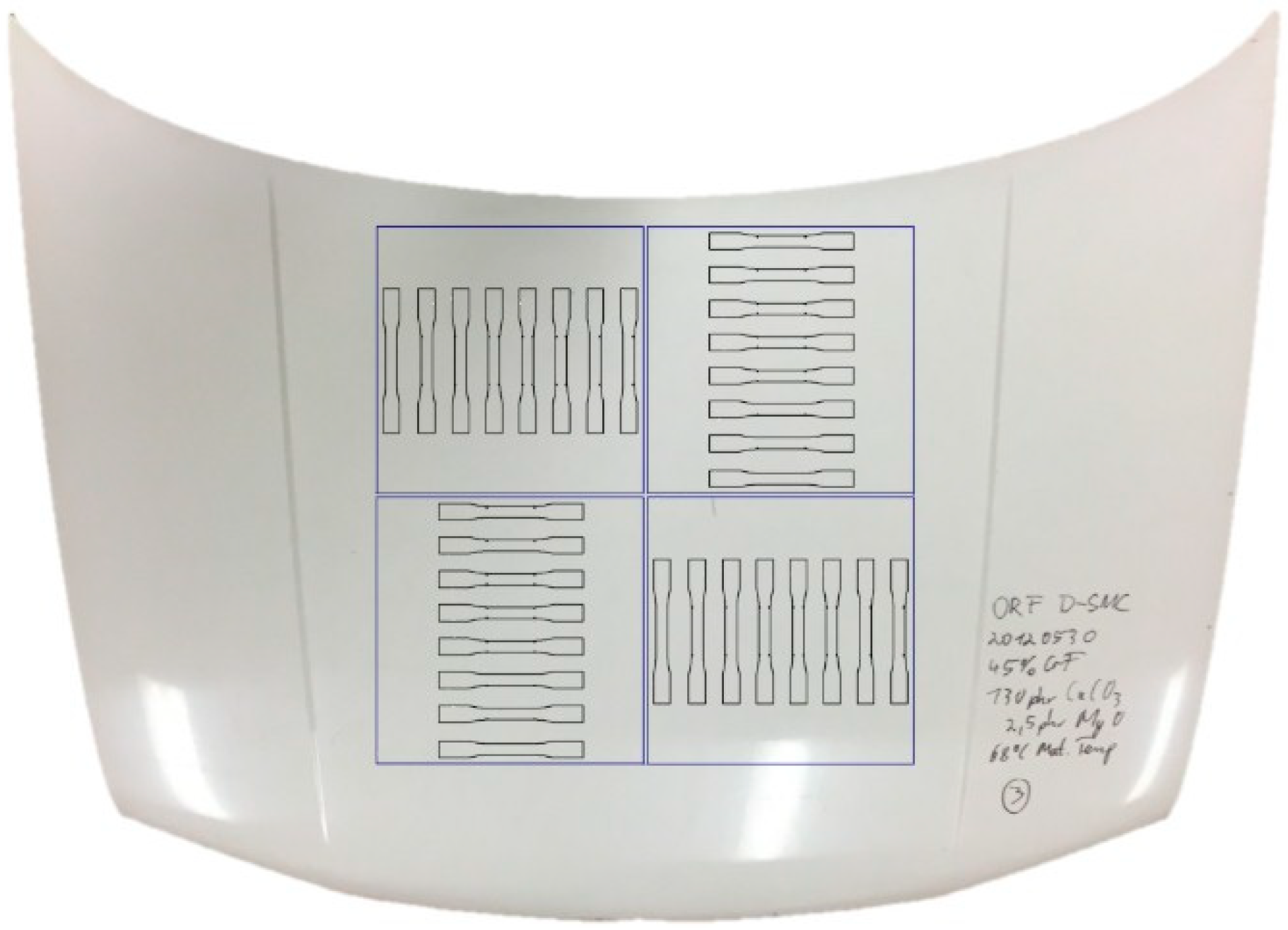
2.1. Material and Manufacturing Process

The materials used for this investigation are car hoods from a sheet moulded compound composite. Two sets of specimens cut from car hoods were tested and analysed; both sets had the same glass fibre reinforcement, matrix material, and fillers, but in different quantities. One set of hoods had a 25% volume fraction of glass fibres, and a PEEK (polyether ether ketone) matrix with 795 phr (per hundred resin) of CaCO3 and 2 phr of MgO as fillers. The second set had a 45% volume fraction of glass fibres and a PEEK matrix with 730 phr of CaCO3 and 3 phr of MgO as fillers.
The car hoods were manufactured at the Fraunhofer Project Centre for Composites Research at Western University [62], using a sheet moulding compound process. For this process, a film is rolled out onto a platform, where it awaits the premixed polymer resin before going through an extruder and then being distributed onto the film. As the film and resin are carried down the platform, several spools of glass fibre are connected to a cutter where the fibres are cut and distributed into the resin below. Once the fibres are distributed throughout the resin, an additional layer of film is placed onto of the resin. Following that, the material goes through a compounder to seal the constituents together. The now singular sheet exits the compounder and is cut to length. A robotic arm then takes the sheet and places it onto a hydraulic press, where it is pressed to the final desired shape.

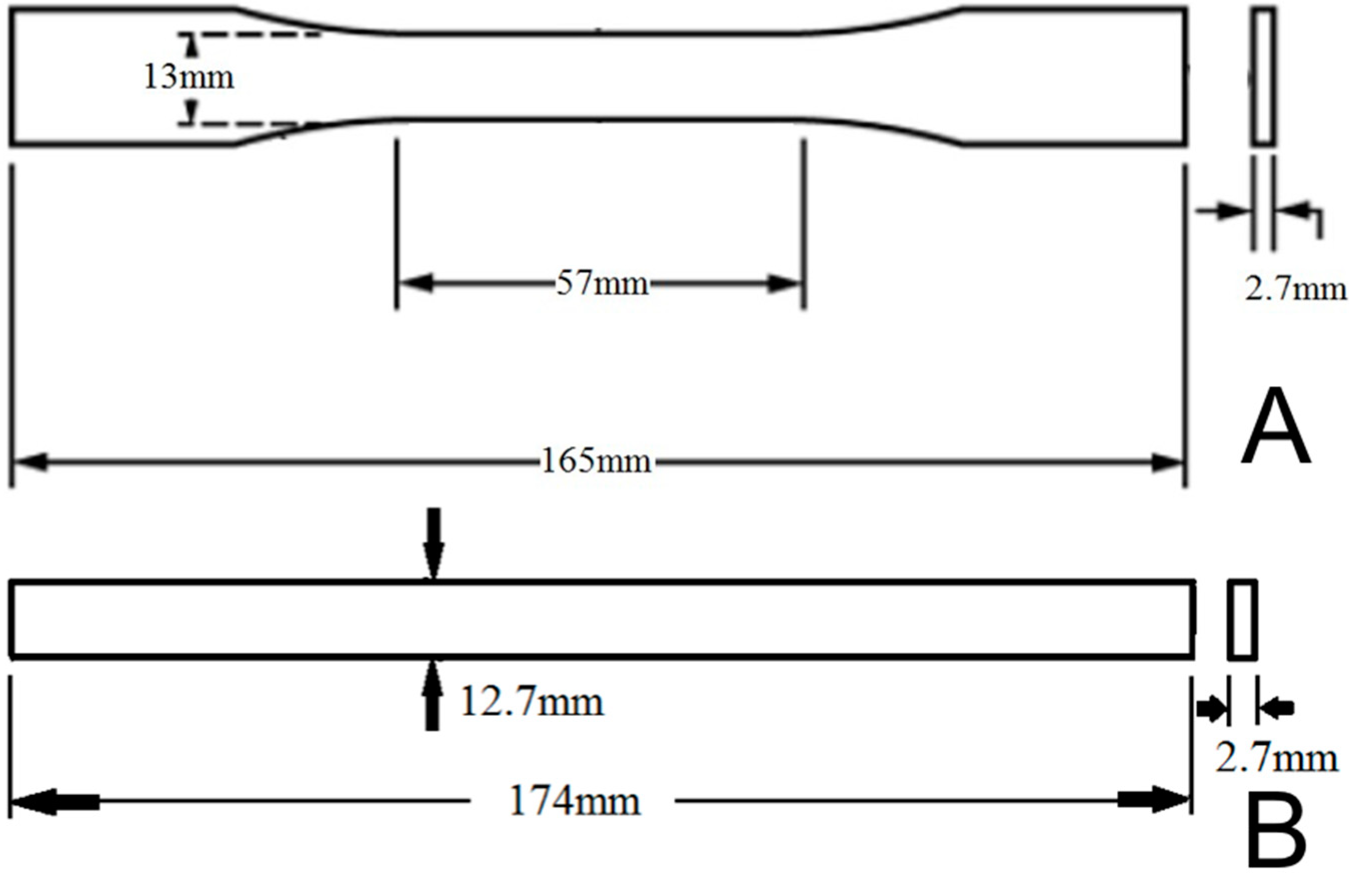
2.2. Specimen Preparation

Both tensile and flexural specimens were prepared for the study. The tensile specimens were machined to ASTM standard D638-14 [63], while the flexural specimens were machined to ASTM standard D790-15 [64]. Dimensional information for the tensile and flexural specimens can be found in Figure 1A,B, respectively. Both types of specimens had similar material preparation; full-sized SMC composite car hoods were cut on a band saw to yield four 305 mm × 305 mm plaques each. These plaques were fastened to a sheet of plywood and placed into a computer numerical control (CNC) to machine the tensile and flexural specimens. Each hood provided both longitudinal and transverse specimens, as seen in Figure 2; although the figure only displays tensile specimens, it should be noted that the flexural specimens were cut from the plaques in the same fashion. ‘Longitudinal’ and ‘transverse’ in this work are in reference to the car hood, not the fibre, due to the randomness of the fibre directions.

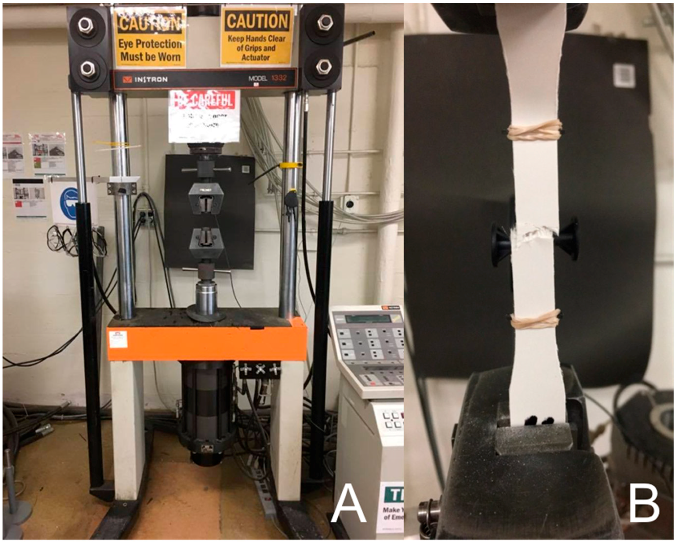
2.3. Uniaxial Tensile Testing

Following specimen preparation, uniaxial tensile tests were performed using the INSTRON model 1332. The INSTRON machine and associated grips for the uniaxial tests can be found in Figure 3A. The INSTRON collected stress data throughout the test, and was used in conjunction with a 50-mm extensometer to accurately record the displacement measurements. The extensometer was attached to the specimens using rubber bands, as seen in Figure 3B.

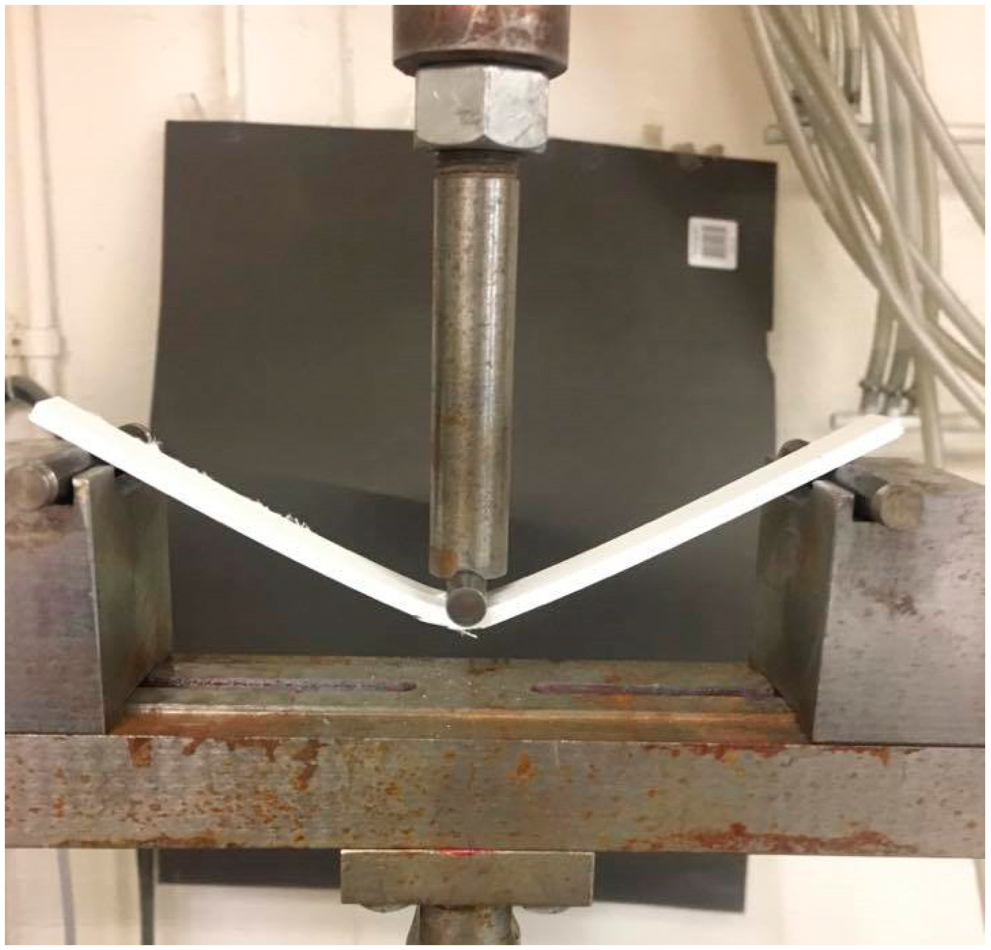
2.4. Flexural Testing

Flexural testing was performed on the INSTRON model 1332 as well, utilising two fixed supports and one loading nose, which is shown in Figure 4. In this experiment, the loading nose was pressed down onto the middle of the flexural specimen until fracture. The loading nose force was recorded by the INSTRON, and the displacement of the nose was used to determine the flexural strain.

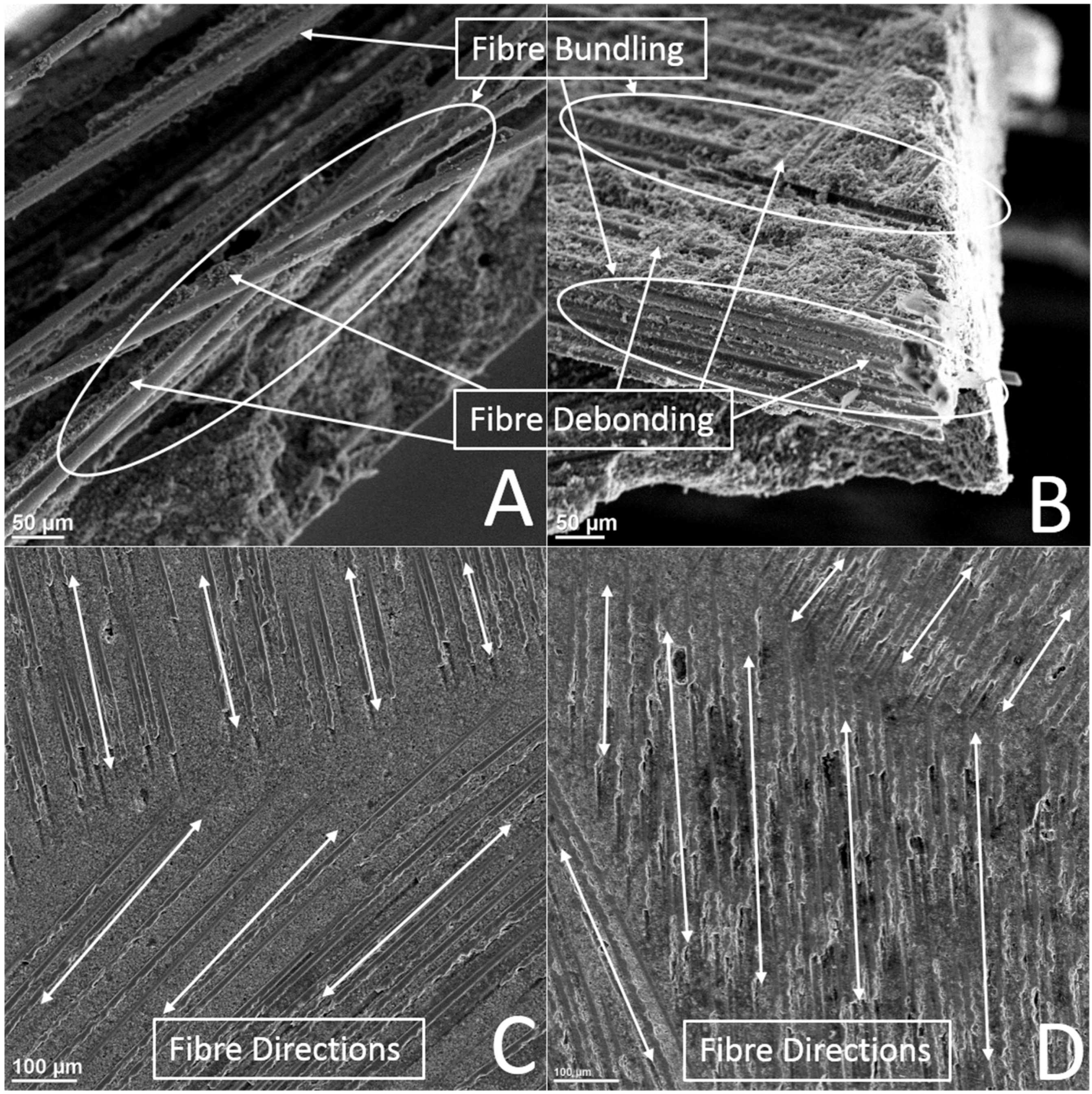
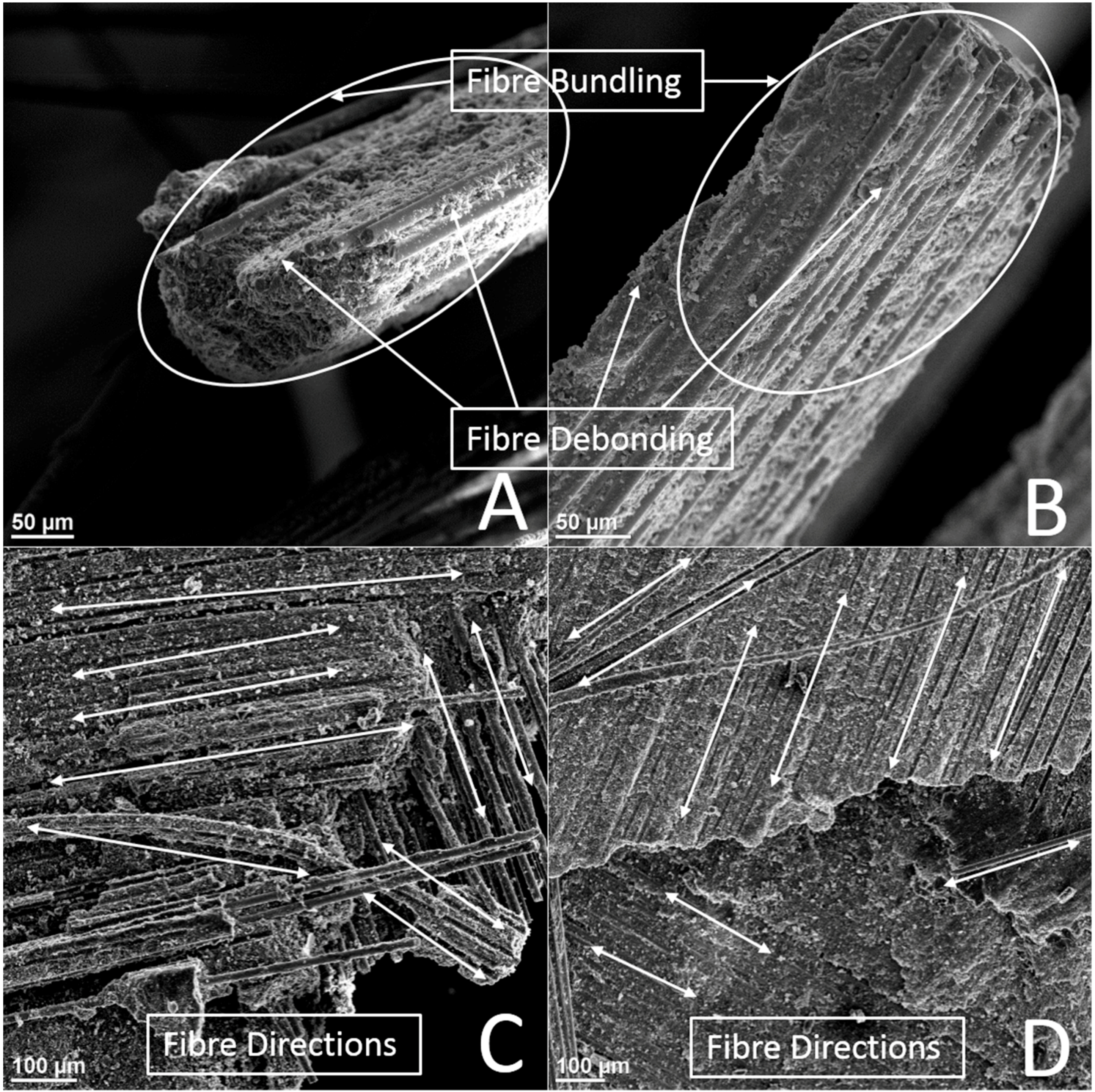
2.5. Scanning Electron Microscopy

The fractured specimens were analysed under a scanning electron microscope (SEM) to further investigate fracture initiation, and help determine the fracture modes of the material. This work was performed in the Microscopy and Microanalysis facility located at the University of New Brunswick (UNB), using a JEOL 6400 SEM system (JEOL USA, Inc., Peabody, MA, USA). Specimens were prepared using the methods presented in a study by Mohammadi and Salimi [65]. Samples of 25% and 45% volume fraction from both the uniaxial and flexural tests were analysed to better understand fibre and matrix interactions.

3. Experimental Results and Discussion

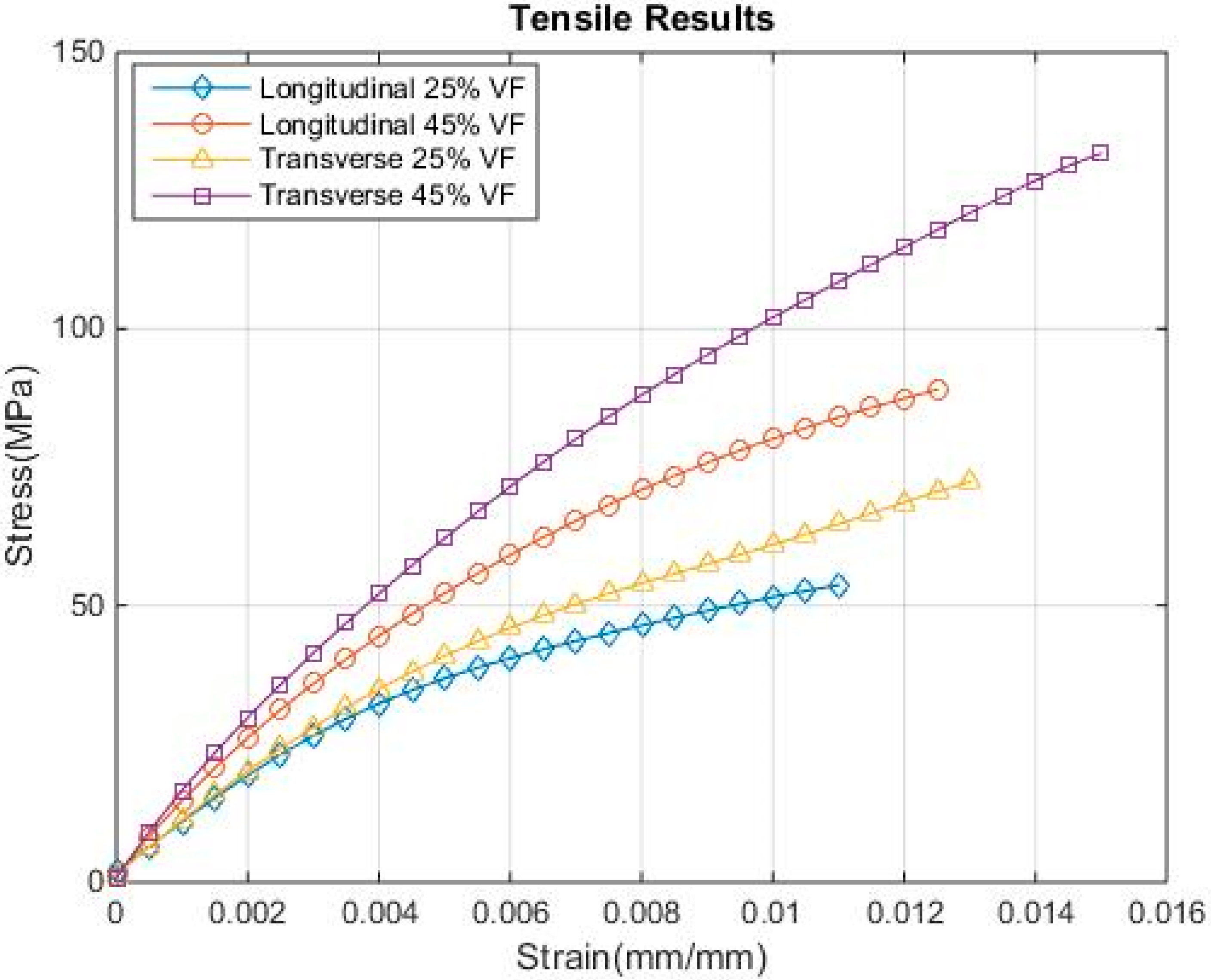
3.1. Uniaxial Tensile Test Results

Uniaxial tensile tests were performed on two different sets of specimens cut from SMC car hoods, with 25% and 45% volume fraction of fibres respectively, in two separate orientations, longitudinal and transverse, yielding four sets of data. Each of the tests was repeated a minimum of eight times to ensure repeatability. The results for each data set were entered into MATLAB software (MATLAB and Statistics Toolbox Release 2012b, The MathWorks INC., Natick, MA, USA), which was used to average the results, producing a single stress–strain curve for each data set. The tests were performed at a strain rate of 3 × 10⁻³ s−1 (all of the uniaxial tensile results with error bars can be found in Appendix A).
Figure 5 displays the experimental results from the uniaxial tensile tests in the longitudinal and transverse directions for both the 25% and 45% volume fraction specimens. First, analysing the longitudinal results, from the figure, it can be clearly seen that the 45% volume fraction specimens displayed superior strength, a higher failure strain, and modulus. This is because the higher fibre content leads to a decrease of the mean glass fibre length, which eventually leads to higher fibre–fibre interaction and higher strength [66]. The 25% volume fraction specimens fractured on average at a stress of 53.7 MPa and averaged a failure strain of 1.10% strain, while the 45% volume fraction specimens fractured on average at a stress of 89.0 MPa and averaged a failure strain of 1.25% strain.
In the transverse results, the same trend as the longitudinal direction is displayed, where the 45% volume fraction specimens fractured at a higher stress, while achieving a greater fracture strain and modulus. It should be noted that the transverse direction exhibits greater failure stress, failure strain, and modulus when compared to the longitudinal specimens of the same volume fraction. This is due to the alignment of more glass fibres in the transverse direction during the manufacturing process, leading to more fibre content concentration and higher strength than the longitudinal direction, see studies by Fu et al. [66] and Kuriger et al. [67]. The 25% volume fraction specimens fractured on average at a stress of 72.4 MPa and averaged a failure strain of 1.30% strain, while the 45% volume fraction specimens fractured on average at a stress of 131.7 MPa and averaged a failure strain of 1.50% strain. The mechanical properties along with the anisotropic behaviour of the SMC composite material that was investigated in this study is comparable with the similar SMC composite produced by the Wetlay process earlier and studied by Lu [68].

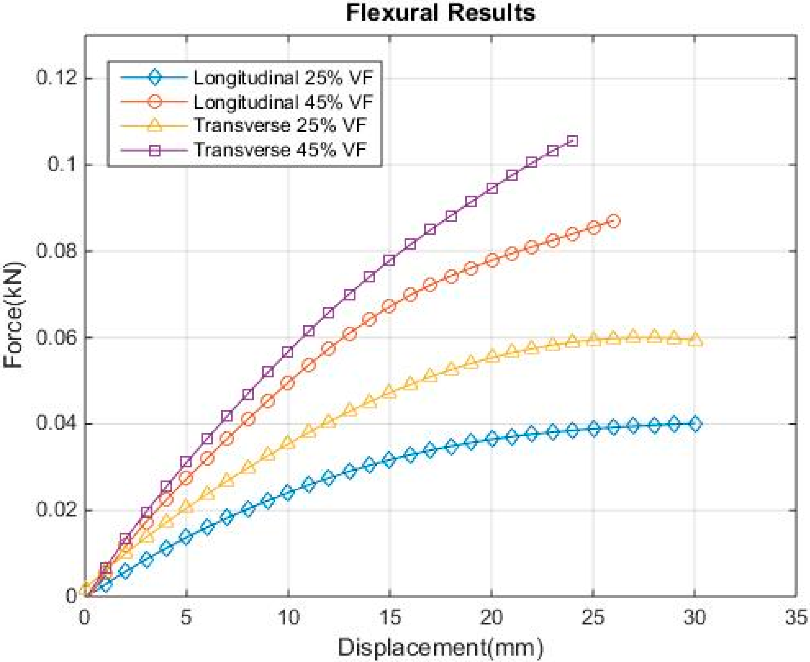
3.2. Three-Point Bending Test Results

The three-point bending tests were performed with the same car hood specimen volume fractions, 25% and 45%, and material directions, longitudinal and transverse. Additionally, the flexural tests were performed a minimum of eight times to ensure their repeatability, and MATLAB was used to average the results. These tests were performed at the same strain rate of 3 × 10⁻³ s−1 or a velocity of 10 mm/min (all of the flexural bending results with error bars can be found in Appendix B).
Figure 6 presents the experimental results from the three-point bending tests in the longitudinal and transverse directions for both the 25% and 45% volume fraction specimens. It is noted that the same trend as was seen for the uniaxial tensile tests can be observed with the flexural tests. First, focussing on the longitudinal tests, the 45% volume fraction specimens had a vastly higher force at failure, which was more than double that seen in the 25% volume fractions, but failed at a lower displacement. The 25% volume fraction specimens on average failed at a force of 40.1 N, and had an average failure displacement of 30 mm. The 45% volume fraction specimens on averaged failed at a force of 87.1 N, and had an average failure displacement of 26 mm. This trend with the flexural properties of SMC composites was seen previously in the studied performed by Thomason and Vlug [69], where higher fibre content led to higher flexural strength.
The flexural behaviour of the transverse samples was very similar to those seen in the longitudinal tests. The 45% volume fraction results fractured at a higher force and a lower displacement than those seen in the 25% volume fraction results. However, the difference in failure force between the 25% and 45% volume fraction specimens is less in the transverse results, while the failure displacement difference is greater. The transverse results displayed higher failure forces than the longitudinal results, while the fracture displacements remained relatively the same. During the manufacturing process, some of the fibres can be aligned in the transverse direction and out of plane due to the randomness and small length of the fibres. Since flexural tests are a combination of tension and compression, some of these fibres are under compressive loads, where a higher stiffness than the longitudinal samples was achieved [69]. This was further verified using the SEM images. The 25% volume fraction specimens on averaged failed at a force of 59.5 N, and had an average failure displacement of 30 mm. The 45% volume fraction specimens on averaged failed at a force of 105.7 N, and had an average failure displacement of 24 mm. Similar to the uniaxial tensile tests, the results obtained for the flexural tests along with the mechanical behaviour of the material were close to the results presented by Lu [68] using the Wetlay process for manufacturing SMC composites.

3.3. Scanning Electron Microscopy Analysis

A scanning electron microscopy (SEM) investigation was put forth to look deeper into the mechanisms of fracture and distinguish the complicated failure modes undergone by short fibre-reinforced composites. SEM analysis was performed on both the tensile and flexural samples post-fracture. This helped to determine if the same failure modes occur in uniaxial tension as they do in bending. Initial observations displayed that there were signs of fibre bundling, which led to matrix debonding, and subsequently, failure.
Figure 7 displays the SEM images from fractured tensile specimens. Due to the randomness of the fibres and the small focus of the SEM, both the transverse and longitudinal results have negligible differences, and therefore, the same conclusions can be drawn. Figure 7A,B depict the cross-section of a 25% and 45% volume fraction specimen fracture surface, respectively, while Figure 7C,D show the top cross-sections of 25% and 45% volume fraction samples, respectively. In Figure 7A, bundles of fibres are clearly depicted, where fibre bundling is one of the leading causes of fibre/matrix debonding in reinforced composites. As the fibres bundle, their available bonding surface area is reduced; therefore, their ability to adhere to the matrix is reduced [11]. Figure 7B displays the same type of fibre bundling, but due to the higher percentage of fibres, they are more concentrated together, forming larger bundles than those seen previously. It is clear that higher fibre content led to higher fibre–fibre interactions, and bundling yielding higher strength [66]. This fibre bundling also led to the fibre/matrix debonding of a group of fibres at once (Figure 7B), which is known as surface debonding, rather than the individual separation of fibres (Figure 7A), which is known as fibre bundle splitting. Figure 7C,D both demonstrate the randomness of the fibre matrix, displaying that in just one small high magnification frame, multiple fibre directions are found in both images. The presence of out of plane-oriented fibres due to the manufacturing process can be seen in these two figures, which was confirmed by Thomason and Vlug [69] earlier. Although both images are very similar in this front, it can be seen that the 45% volume fraction sample has a much higher concentration of fibres, as expected.
Figure 8 displays the SEM images of fractured flexural specimens. Figure 8A,B show the fractured surface cross-sections of 25% and 45% volume fraction samples, respectively, while Figure 8C,D show the top cross-sections of the fracture surface for 25% and 45% volume fraction samples, respectively. In Figure 8A,B, the same type of fibre bundling and fibre/matrix debonding that was experienced in the tensile specimens can be observed, although in this image, it was more common to find bundles of fibres debonding from other fibre bundles, rather than individual debonding fibres. This is due to the complex nature of the flexural test, which ensures that a combination of tension and compression is present, leading to out of plane oriented-fibre bundles to debond [69]. The only difference seen between the two images in Figure 8A,B is the fibre percentages; the general failure mechanics appear the same. Figure 8C,D display the top cross-sections of the specimens, and similar to observations from the tensile images, these figures display multiple fibre directions in just a small surface area, which demonstrates the fibre direction randomness that is seen throughout the entire part. Here, we also see fibres that have been bent and demonstrate curvature, although these curved fibres still appear to be debonding in larger bundles of fibres, rather than individually. This is because both ends of the short fibres cannot be fully stressed in comparison with long fibres, leading to fibre bundling and further debonding [70].

3.4. Remarks on Fracture

Through careful analysis of the SEM images provided along with the flexural and tensile test results, it can be stated with confidence that the main mode of failure for this SMC composite material has been fibre bundling, leading to matrix/fibre debonding. These findings agree with other studies on this topic in literature, see Matzenmiller et al. [11], Fu et al. [66], Kuriger et al. [67], Lu [68], Thomason and Vlug [69], Baxter [70] and Aboudi et al. [71]. This can help explain the differences between the failure stress and strains seen between the 25% and 45% volume fraction experimental results. In the 25% volume fraction specimens, there is more individual fibre separation seen; therefore, the fibres are not all breaking at once. The 45% volume fraction specimens see groups (bundles) of fibres failing at once, making these failures more catastrophic, and likely the specimen fractured as soon as one of these bundle separations began to occur. The 25% volume fraction samples are not able to reach as high of a stress, since more stress is being put on each fibre, making them fail at lower stresses and lower strains, while the 45% volume fraction samples are able to reach higher stress and higher strains, since there are more fibres to distribute the load and keep the specimen intact. However, once separation occurs it is a rapid failure.

4. Finite Element Model Development

4.1. Model Development and Calibration

The model was developed using commercial FE software LS DYNA (LS-DYNA R8.0, LSTC, Livermore, CA, USA) and experimental data from the uniaxial tensile tests. For each material type, i.e., volume fraction and direction, a different model was created, since the material properties differ for each direction and volume fraction. This work began by 3D modelling the tensile specimen using Autodesk Inventor, and importing that 3D model into LS-PrePost as an IGS file. The specimen was then meshed using solid elements with three layers of elements through the thickness. The mesh was chosen so that each element was approximately 1 mm. A mesh sensitivity analysis was conducted to verify the choice of element size, as presented in Section 4.2. Figure 9 shows the tensile specimen used with nearly constant element size used throughout.
Several material models were tested to predict the deformation of the SMC composite, but material model (MAT_24) Linear Piecewise Plasticity was chosen, as it was the most effective by allowing for experimental stress–strain data to be a material input. Other material models considered include: (MAT_6) Viscoelastic, (MAT_19) Strain Rate Dependent Plasticity, (MAT_22) Composite Damage, (MAT_64) Rate Sensitive Power law Plasticity, and (MAT_76) General Viscoelastic. While these models produced encouraging results, the unique deformation pattern of the composite material required a material model that was able to precisely capture the stress–strain behaviour, and for that reason, MAT_24 was chosen. MAT_24 utilises both elastics properties and effective plastic stress–strain curves as inputs for calculating material responses. The model utilises the elastic properties with elastic equations to calculate the initial material response, but as the material reaches the yield point and transitions from elastic to plastic, the material model transitions to the inputted effective plastic curve to calculate the plastic response.
After the specimen was assigned a material mesh (aligned with the x-coordinate direction), the boundary conditions were put in place to replicate the uniaxial test. The x = 0 end of the specimen was prescribed nodal constraints to prevent rotation or displacement in any direction. At the x = L end, element nodes were given a degree of freedom in the x-direction only, and assigned a nodal velocity to correlate to the testing strain rate of 3 × 10⁻³ s−1.
The model material properties were the next task in the simulation process. For this, the density, Young’s modulus, Poisson’s ratio, yield stress, and failure strain were measured and prescribed as material inputs. The density, Poisson’s ratio, and failure strain were extracted from experimental test data. Due to the viscoelastic nature of the material, and the non-distinct yield point possessed by thermosets [72], Young’s modulus and yield properties could not accurately be determined from experimental testing alone; therefore, they had to be calibrated using the finite element method (FEM). This was done by beginning with calculated estimates and iteratively adjusting the Young’s Modulus and yield the stress to best match the experimental data. For this type of model, the plastic deformation can be simulated very accurately, but it requires a logical elastic deformation zone as defined by the linear plastic model. This type of elastic deformation is not present in SMC composites, as there is no distinct elastic to plastic transition, as would be seen on a typical stress–strain curve. This is the reason that iteration was needed to determine the Young’s modulus and yield stress. The Young’s modulus was increased gradually, while the yield stress was progressively set to occur at earlier strain values, so that the combinations of the two would result in a smooth transition from elastic deformation to the user-defined plastic deformation. This resulted in less accuracy in the elastic portion of the curve, but resulted in a much more accurate plastic deformation zone, which is of greater interest to the study. Each model was calibrated separately, and the resulting properties can be found in Table 1. Material orientations are designated with an ‘L’ for longitudinal or ‘T’ for transverse (in reference to the direction of the hood and not fibre directions), along with the volume fraction of fibres.
The results for the longitudinal and transverse uniaxial tensile simulations can be found in Figure 10 and Figure 11, respectively. Both the 25% and 45% volume fraction’s actual and predicted stress–strain data are presented on the same plot. Here, both the longitudinal and transverse uniaxial tensile tests are exhibiting the same type of behaviour. The 25% volume fraction simulations are accurate for the majority of the simulation, and in particular at higher strains, but there is minor overprediction prior to 0.5% strain, with a maximum error of 2.3 MPa and 4.3 MPa for the longitudinal and transverse directions, respectively. The same result is seen in both the 45% volume fraction simulations, although there is a larger overprediction at the low strain region of the curve (maximum error of 5.7 MPa and 9 MPa for the longitudinal and transverse directions, respectively) compared to the 25% volume fraction simulations, and the curves converge between 0.6% and 0.7% strain. The longitudinal and transverse 25% volume fraction simulations had root mean square (RMS) errors of 0.99 MPa and 1.97 MPa, respectively, while the longitudinal and transverse 45% volume fraction simulations had RMS errors of 2.98 MPa and 4.00 MPa, respectively.
An explanation for the separation at low strains can be that the material model used is a plasticity model, which assumes that there is a clear and sudden elastic–plastic transition, but that is not the case for this SMC composite. The transition from elastic to plastic for this material, similar to thermosets, is gradual and cannot be defined by a single parameter. The plastic model also assumes that the work hardening is due to slip, while the SMC material deviates from pure elastic due to debonding and the breaking of fibres causing damage that weakens the material. Additionally, the elastic properties are greater in the 45% volume fraction models, explaining why there is a greater separation seen in the elastic portion of those simulations. Calibration of the models was iteratively conducted to determine the input material properties so that the high strain region of the curve would be more accurate, since this is the part of the curve that is of the most interest.
The experimental and simulated values for ultimate tensile strength (UTS) and fracture strain are presented in Table 2. From these results, it can be seen that the fracture strains from all of the simulations matched the experimental results well, and the ultimate tensile strength also matched well to within 2% error.

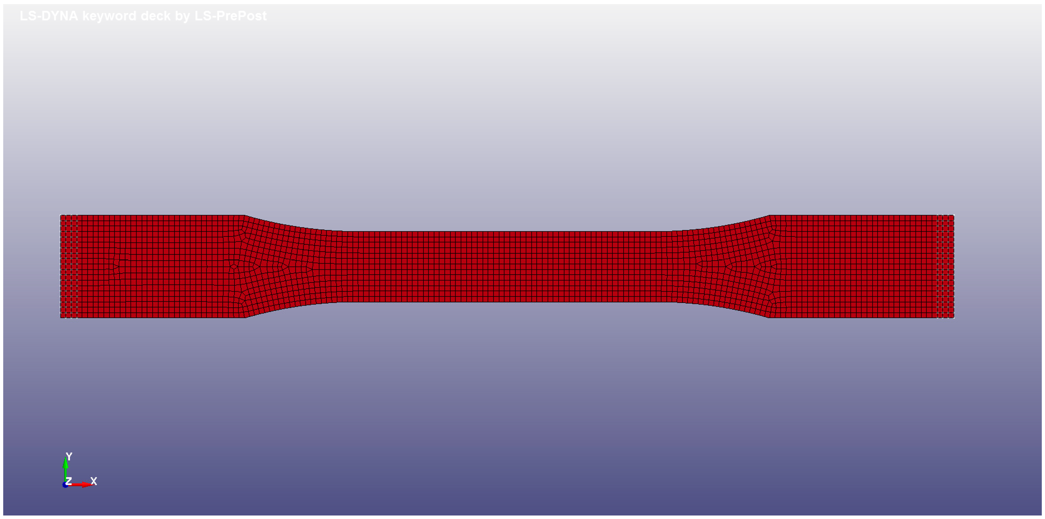
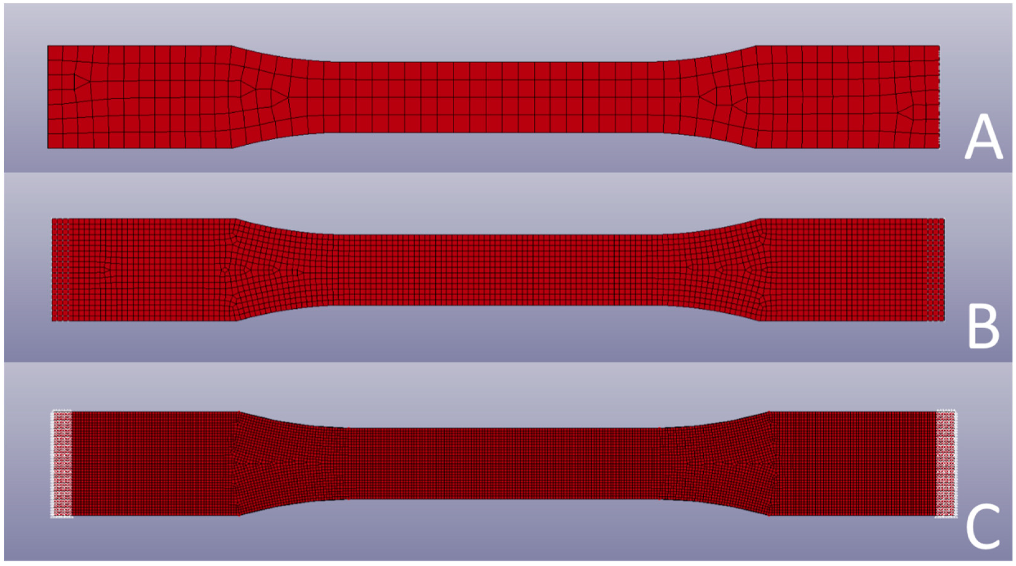
4.2. Mesh Sensitivity

Mesh sensitivity analysis was performed on the simulation in order to eliminate the effects of mesh size on the computed results. Figure 12 shows the three mesh sizes tested in this work. The stress–strain curves were found not to be sensitive to mesh size, but the failure strain was. Table 3 displays the comparison of ultimate tensile strength and failure strain for each mesh tested. The chosen mesh was determined according to failure strain’s mesh-dependency [73].

4.3. Overview

This model makes use of experimental tensile results of specimens that were cut from SMC car hoods in two different material orientations: longitudinal and transverse. A series of specimens were tested for each material orientation; those results were then averaged and used to produce a finite element model. A finite model was created for each of the material orientations, so that in future works, an anisoptropic model can be applied to the entire car hoods, while using these models as inputs for the longitudinal and transverse orientations.

5. Model Validation and Further Discussion

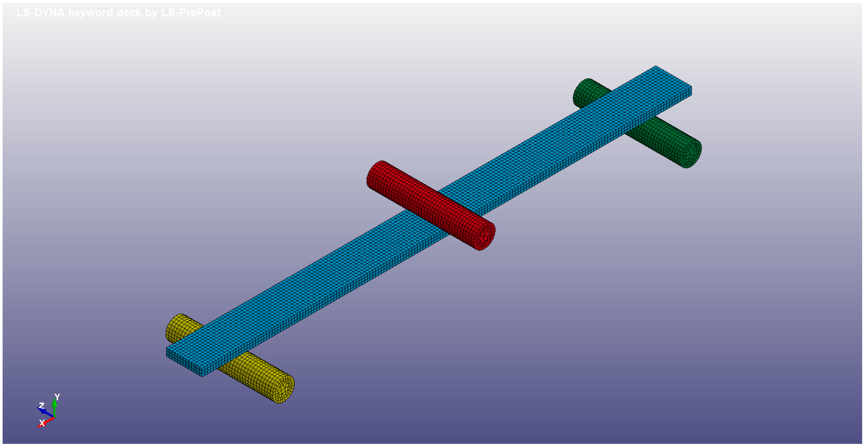
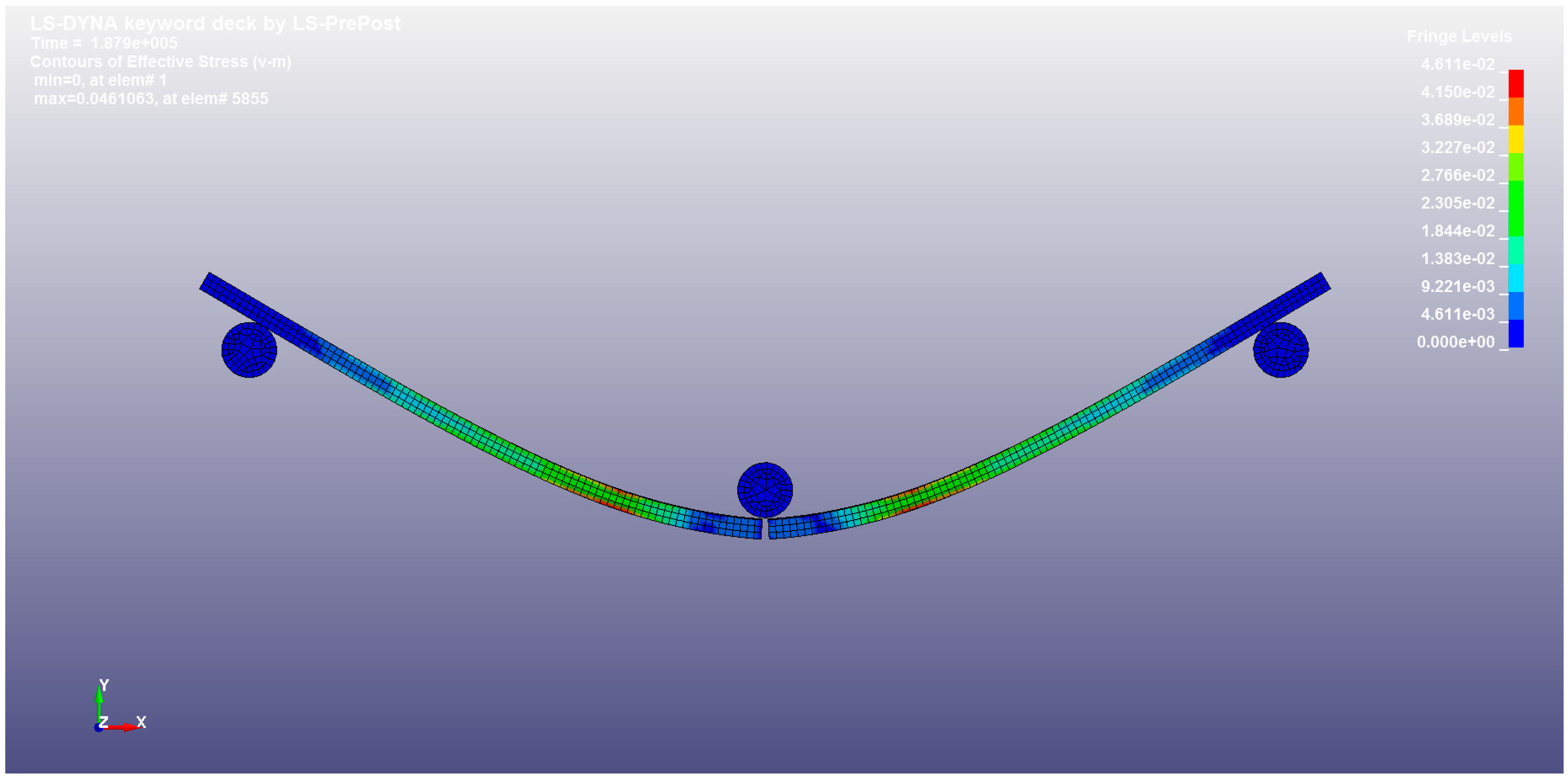
5.1. Flexural Model Setup

To validate the simulation framework presented earlier, each uniaxial tensile model was used to simulate the associated material response in three-point bending tests. The three-point bending simulations used cylindrical supports and a loading nose meshed as rigid parts to govern the bend deformation, rather than the nodal constraints used in the tension simulations. The model was assembled in an Autodesk Inventor prior to being imported into LS-DYNA PrePost (Livermore Software Technology Corp., Livermore, CA, USA) and meshed with solid elements. The same mesh size was used as the ones in the uniaxial tensile simulations. The meshed flexural model can be seen in Figure 13.
The supports and loading nose were assigned the same mesh size as the flexural specimen to ensure smooth and more stable simulations [74]. Three surface-to-surface contacts were defined: one between the loading nose and the flexural specimen, and one between each of the supports and the flexural specimen. The friction coefficients at each contact are summarised in Table 4, as determined from the literature [71]. The flexural specimen was not constrained beyond contact with the supports and the load applied by the nose. Each of the supports was fixed, while the loading nose had translational freedom in the y-direction only.
Although the objective of simulating the flexural response of the material with the previously developed tensile model was validation, some modifications for the definitions of contact still needed to be made. First, the previous model did not have any contact; therefore, both contact and global dampening needed to be added to the model. Second, a failure criterion based on failure strain was added to the tensile model to accommodate failure. The two types of tests (uniaxial tensile and flexural) activate failure mechanisms at different strain levels. In addition, the presence of global damping adds computational stiffness to the model, which affects the onset of failure. This can be understood because of the more complex state of strain in the flexural case, and the local behaviour of strain in the matrix [75]. Therefore, the failure strain was recalibrated for the flexural model. The failure strain values for both the tensile and flexural model can be found in Table 5. From this table, it can be seen that the 25% volume fraction models had a greater difference between the failure strains in the tensile model versus the flexural model. This was because the 45% volume fraction models were found to have more vibration noise at the beginning of the simulation and needed additional damping to smoothen the initial contact. Furthermore, there was some sliding that occurred between the supports and the specimen. This frictional force needed dampening as well to smoothen the noise that aroused from the contact and sliding, and also to capture the real bending phenomenon during simulation [76]. This can be confirmed from Figure 4, where the specimen had gradually been sliding along the supports throughout the flexural tests.

5.2. Flexural Test Simulations

The results for the flexural longitudinal and transverse simulations are shown in Figure 14 and Figure 15, respectively. The longitudinal result for the 25% volume fraction matched the experimental data the best, having minor overprediction prior to 15 mm of displacement, (maximum error of 4.1 N) and converging thereafter. The transverse 25% volume fraction simulation results were not as accurate as the longitudinal results, having a maximum error of 5.7 N happening in the beginning of the flexural test, where the contact condition is not in its steady condition. However, the flexural simulations were very accurate in terms of predicting the failure displacement and force. The curves did converge once at approximately 12 mm of displacement, and did not converge again until fracture. There was a similar result seen in both of the 45% volume fraction simulations, which were much less accurate than those seen in the 25% volume fraction simulations. The 45% volume fractions had a larger separation at the beginning of the force displacement curve, having a maximum error of 17.6 N and 19.1 N for the longitudinal and transverse directions, respectively. It is clear that the 45% volume fraction simulations experienced a much higher tangent modulus. The 45% volume fraction curves do later converge once, and the resulting failure displacement is accurate, but the failure force experienced an increased error compared to that seen in other simulations, differing by 4.2% and 6.6% for the longitudinal and transverse models, respectively. The RMS error was calculated over several points through the curves, and was found to be 1.53 N and 3.39 N for the 25% volume fraction longitudinal and transverse directions, respectively, while the RMS error for the 45% volume fraction simulations was 6.22 N and 6.74 N for the longitudinal and transverse directions, respectively.
Figure 16 displays a fractured flexural specimen from the longitudinal 25% volume fraction simulation. This figure captures the specimen just as it begins to fracture in the centre of the piece (as seen in Figure 4), while the colour scale displays that the part failed at an equivalent Von Mises stress of approximately 46 MPa, which translates to a failure force of approximately 40 N.
The flexural simulation and experimental results are presented in Table 6. The displacement at failure was mostly accurate in all of the simulation results, differing between the simulation and experimental value by 2.5% or less in all of the simulations. The failure force was the less accurate parameter, but the results were positive still. The longitudinal failure force results differed by 1.5% and 4.2% for the 25% and 45% volume fraction models, respectively, while the transverse results differed by 3.5% and 6.6% for the 25% and 45% volume fraction models, respectively. This model demonstrates accuracy similar to those of the other predictive models that have been used to predict composite material behaviour [77,78,79].

5.3. Remarks on the Accuracy of the Results

From the results above, it is clear that the model becomes less accurate in simulations with higher forces. The simulations at higher forces are also those that have higher volume fraction percentages, and with higher volume percentages, there is a greater chance of fibre-related failure modes to occur: either fibre bundling and kinking, or fibre rupture. These failure modes can cause localised failure, which leads to the part failing before it reaches its ultimate tensile strain, making the properties of higher fibre composites less predictable [71]. Another potential source of error is that the bending model was generated from a tensile finite model, which means that the tensile properties of the material are accounted for, but the compression behaviour is not. Compression is a significant portion of the three-point bending test, as the failure stress could come from the top or bottom of the specimen [70]. If the fracture happens at the bottom of the flexural specimen, then the tensile properties govern failure, but if it fractures on the top section of the part, compression would be the instigator of failure.
The main source of inaccuracy seen throughout these simulations is the first half of the force displacement curves in the 45% volume fraction simulations. While there was separation seen at the beginning of every curve, the separation seen in the 45% volume fraction simulations was significantly greater. From Figure 8, it can clearly be seen that there are many different fibre orientations seen throughout the material, and as the specimen is loaded, these fibres begin to distribute the load amongst each other. In the experiments, these fibres would not all take the same load [70], and they would not all be in the most favourable loading direction [67], but the simulation cannot take this into account. It was assumed that the fibres would all be taking the same load throughout the simulation. However, this is not the case in reality, and for this reason, there is a large separation at the beginning of the curve. It can be seen that as the material deforms, the simulation converges towards the experimental data curve. This is because the material input given to the model would overpredict the force at the beginning of the simulation due to the uneven loading seen at the initial stages. The fibres and matrix fail during material deformation [11], where this weakens the composite. It can be seen that the model takes this failure into consideration as the simulation curves quickly decline and begin to match the experimental data. However, it is the model’s inability to account for the lack of fibres loaded at the beginning of the simulations [70] causing the inaccuracy.
Overall, the model was successful, being able to predict the deformation of the 25% volume fraction specimens with at most a 3.5% error (in reference to failure strain and failure force), and the 45% volume fraction specimens with at most a 6.6% error. A micromechanics model as developed earlier for long fibre-reinforced composites by Sabiston et al. [43,45] based on the random characteristics of the SMC composites can help to capture these errors mainly for the longitudinal and transverse 45% volume fraction samples.

6. Conclusions

Multiple series of both uniaxial tensile and flexural bending tests were performed on SMC composite specimens from an SMC car hood to quantify the mechanical characteristics of the material. The study produced a collection of results for the 25% and 45% volume fraction samples for both the longitudinal and transverse directions, where both the tensile and flexural tests were performed at a strain rate of 3 × 10⁻³ s−1. Scanning electron microscopy was performed to study the fracture surface and aid in determining the primary failure modes of the composite. These results were used to determine the mechanical properties for the material, so that a finite element model could be developed. The tensile results were used to develop and calibrate the finite element model to describe the deformation of the SMC composite. The flexural results were then used to validate the model and predict the bending behaviour of these composites. The following conclusions can be drawn from the current work based on the experiments and simulations performed in this study:
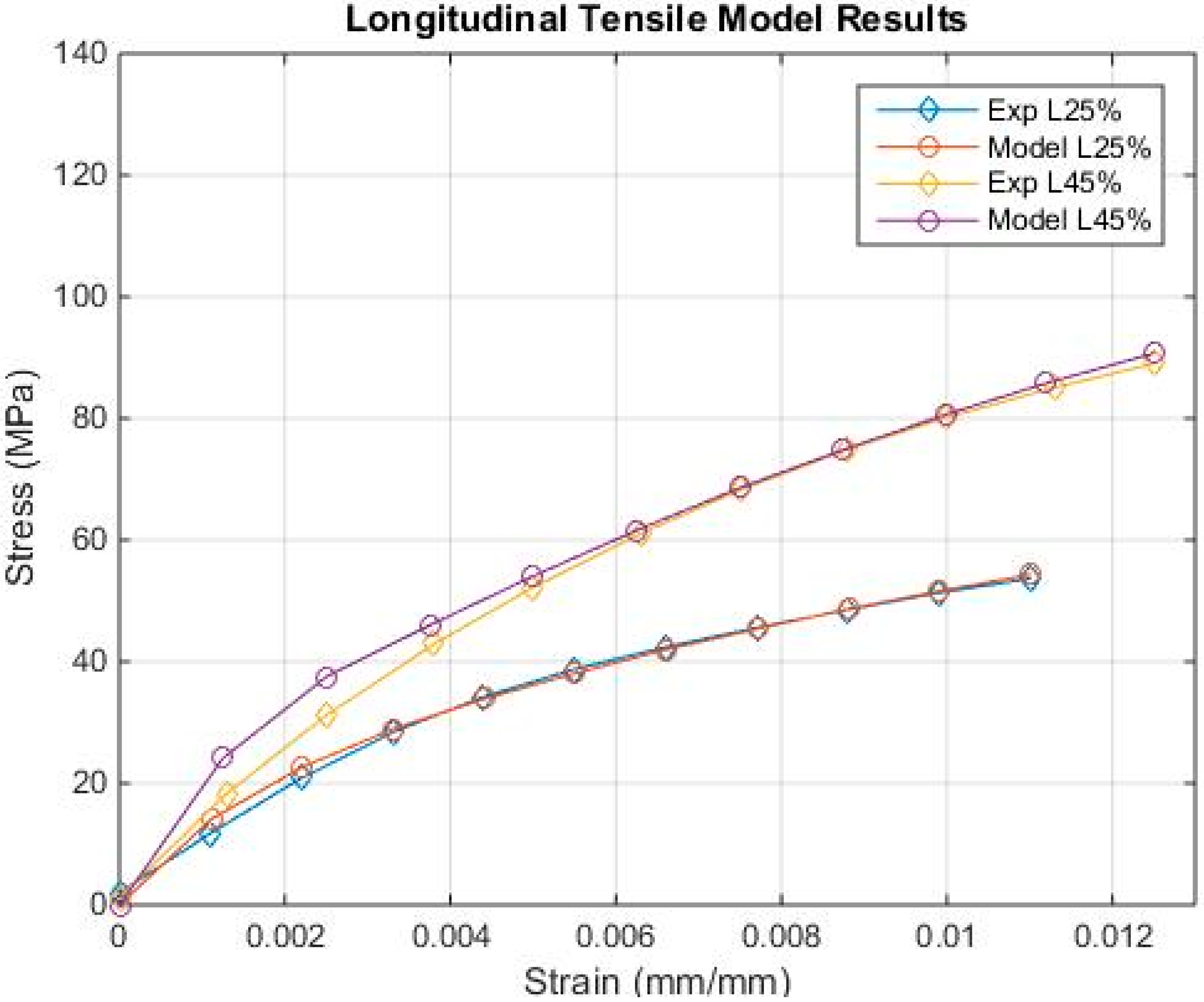
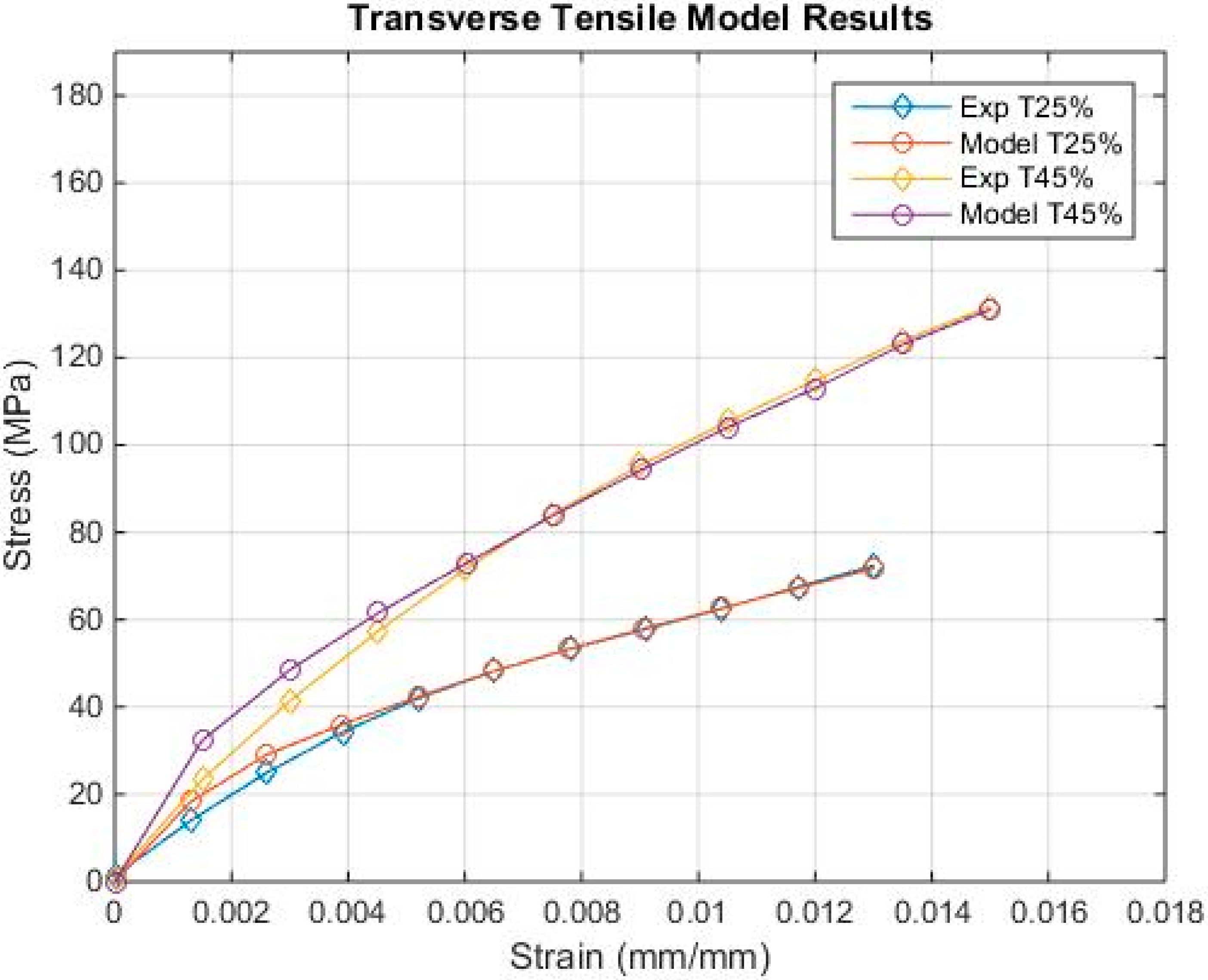
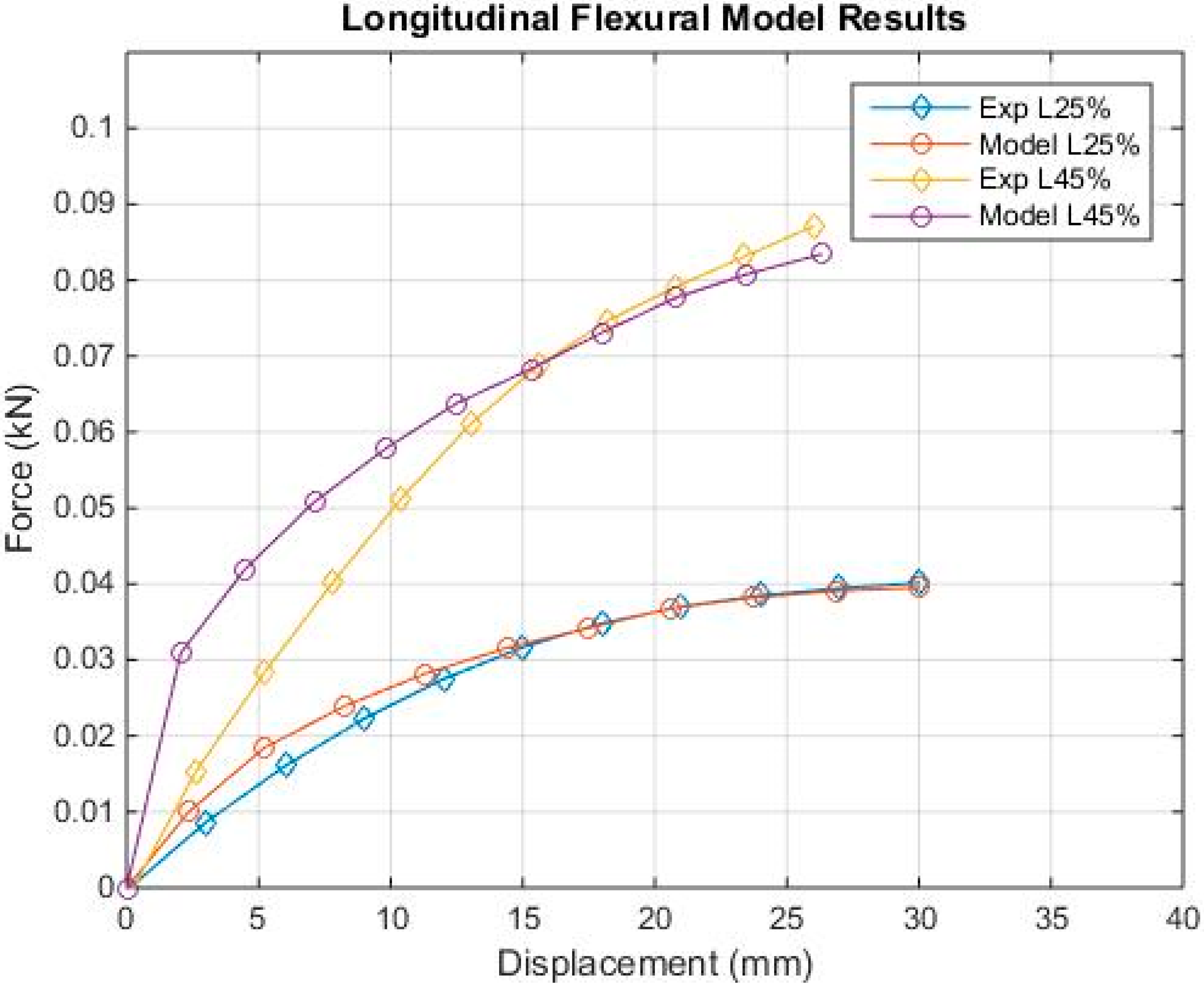
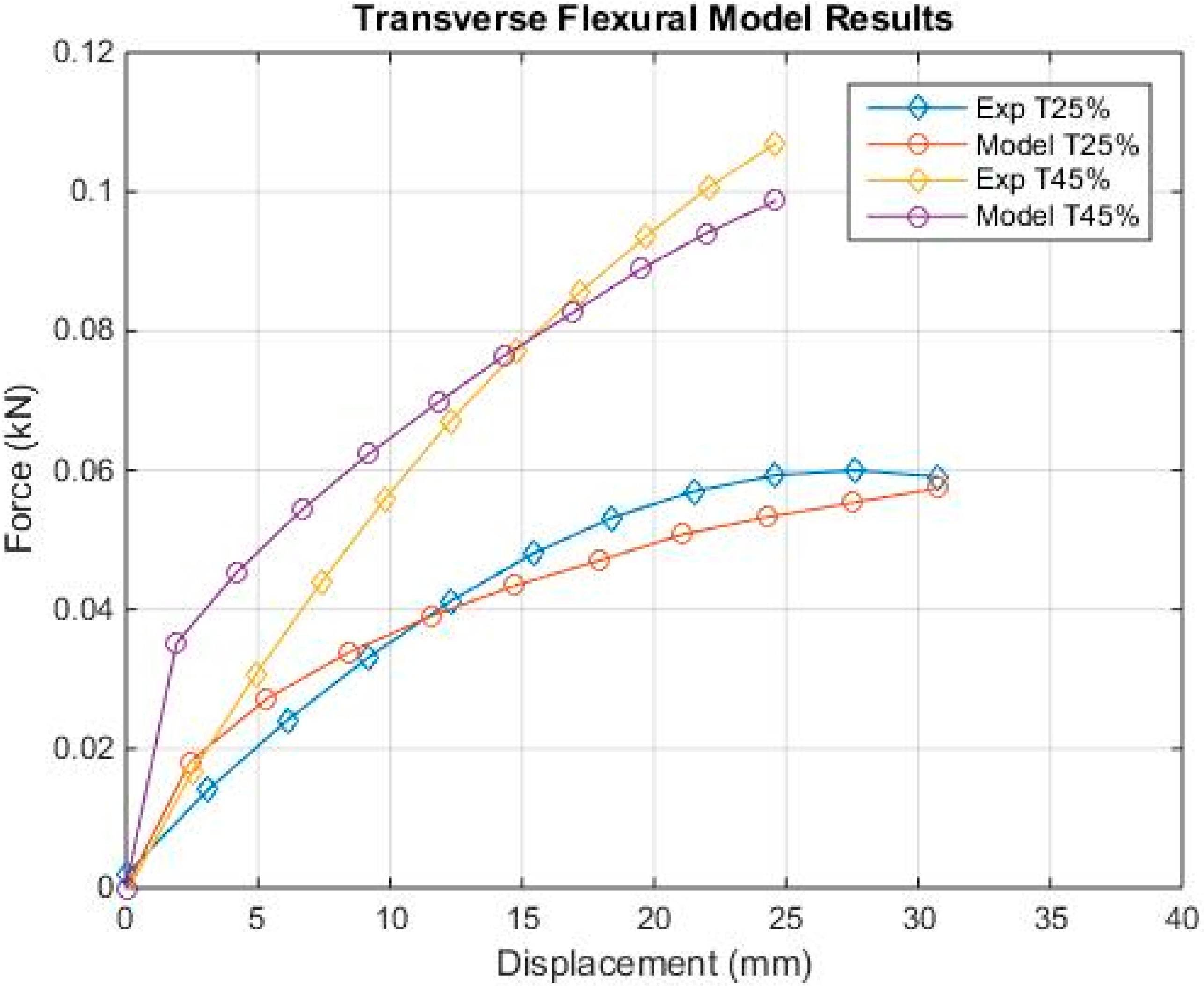
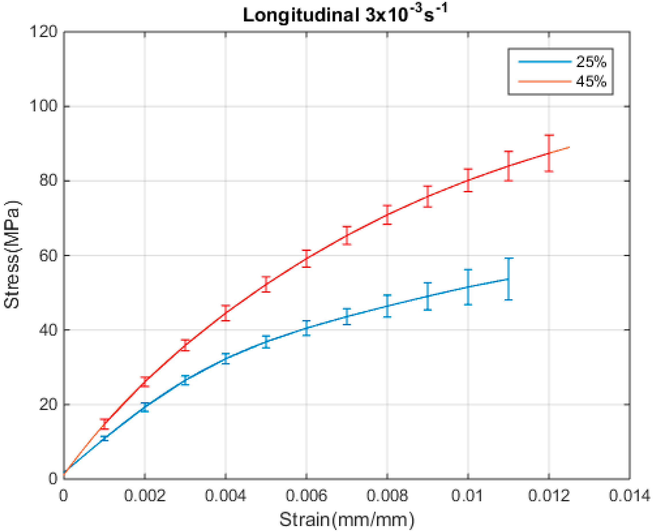
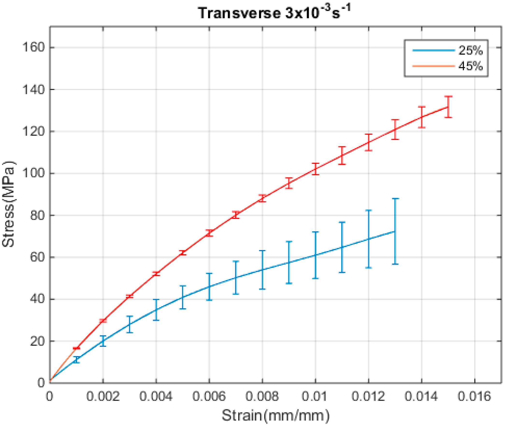
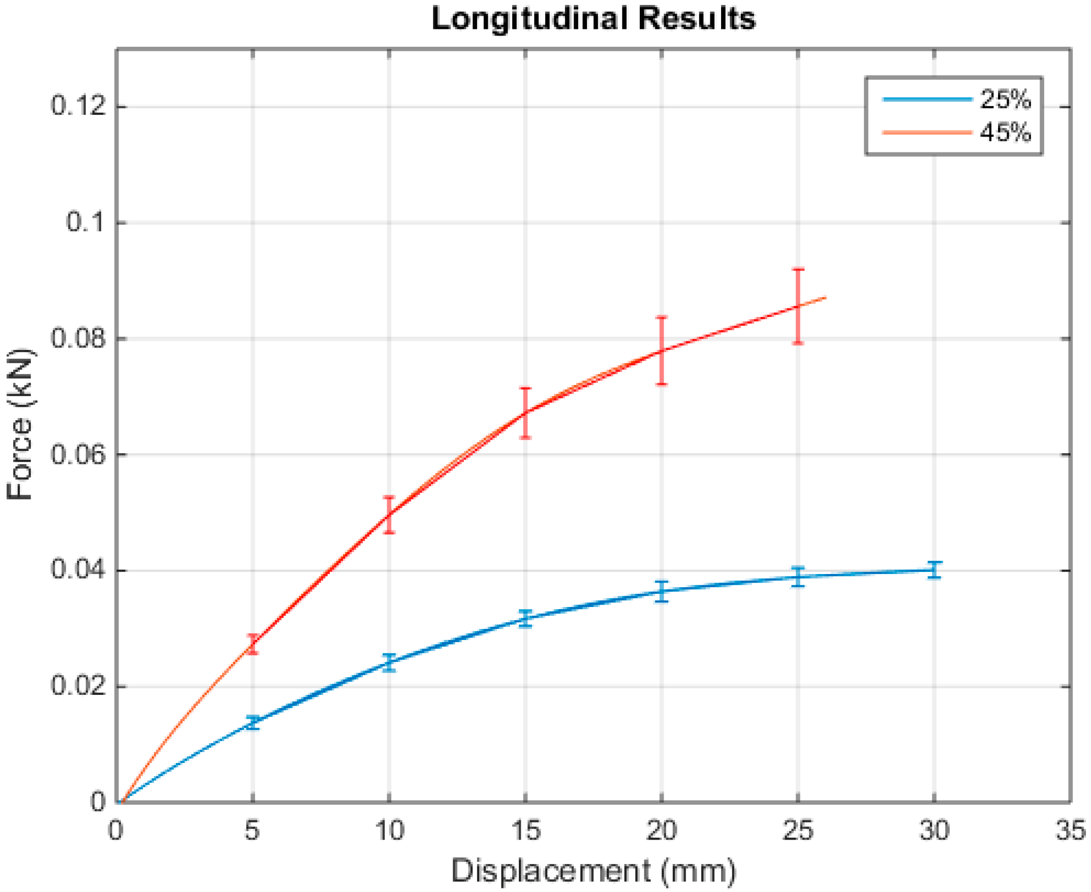
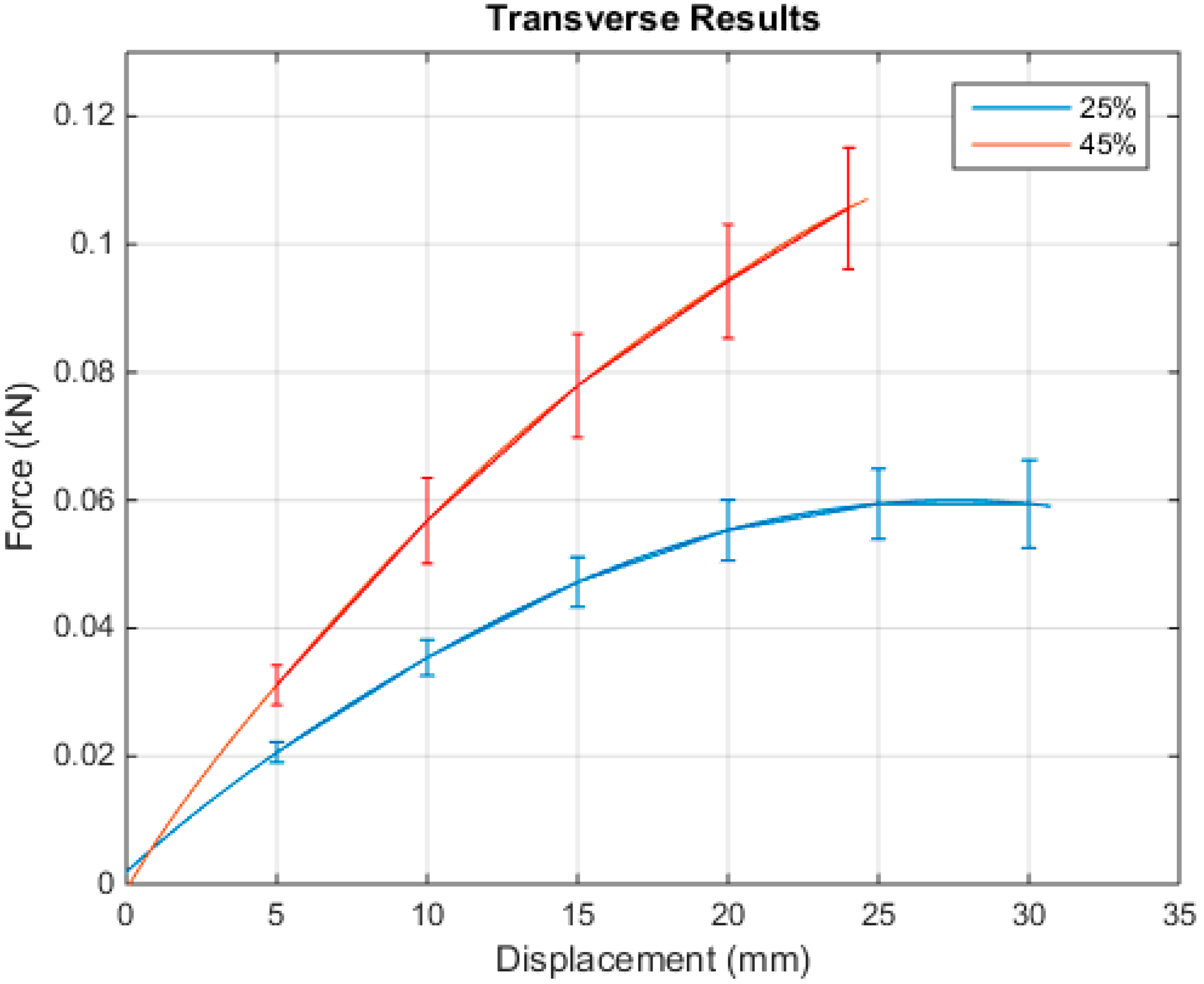
  • Throughout the tensile tests, the higher volume fractions led to a higher UTS and failure strain, while the transverse direction was stronger than the longitudinal direction. The flexural test saw similar results, with the higher volume fraction specimens reaching a higher failure force, but the failure displacement was less than that seen in the lower volume fraction tests; however, again, the transverse direction proved to be stronger than the longitudinal direction.
  • The SEM images taken lead to the conclusion that fibre bundling leading to matrix debonding is the primary failure mode of fracture in both the 25% and 45% volume fraction specimens, for the tensile and flexural tests.
  • A linear piecewise plasticity material model was able to simulate very well the tensile stress–strain data for calibration, and provide good results. The model was then validated by simulating the three-point bending tests along with the experimental flexural data. The lower volume fraction simulation was more accurate than the higher volume fraction simulation, with a maximum error of 3.5% for the 25% volume fraction tests, and 6.6% for the 45% volume fraction tests. The reason that the 45% volume fraction simulations are less accurate is that the model cannot account for the uneven loading of fibres experienced at the beginning of the flexural tests. This is an area that should be investigated further in future work using micromechanics-based models.

Author Contributions

Investigation: J.K.; Validation: E.C., Supervision: M.M.

Acknowledgments

The Authors would like to thank Natural Sciences and Engineering Research Council of Canada (NSERC) grant number RGPIN-2016-04221 and New Brunswick Innovation Foundation (NBIF) grant number RAI 2016-108 for providing sufficient funding to execute this work. In addition, the authors would like to thank Jeff Wood (Western University) and Fraunhofer Project Centre for Composites Research in London, Ontario for providing the composite car hoods. Finally the authors would like the thank technicians Brian Guidry, Bob MacAllister, and Vince Boardman, without their help this project would not be possible.

Conflicts of Interest

The authors declare no conflict of interest.

Appendix A. Uniaxial Tensile Tests with Error Bars

Figure A1. Longitudinal 25% and 45% 3 × 10⁻³ s−1 Results with Standard Deviation Error Bars.
Jcs 02 00053 g0a1
Figure A2. Transverse 25% and 45% 3 × 10⁻³ s−1 Results with Standard Deviation Error Bars.
Jcs 02 00053 g0a2

Appendix B. Flexural Bending Tests with Error Bars

Figure A3. Longitudinal Results with Standard Deviation Error Bars.
Jcs 02 00053 g0a3
Figure A4. Transverse Results with Standard Deviation Error Bars.
Jcs 02 00053 g0a4

References

  1. Jayasree, N.A.; Airale, A.G.; Ferraris, A.; Messana, A.; Sisca, L.; Carello, M. Process analysis for structural optimisation of thermoplastic composite component using the building block approach. Compos. Part B 2017, 126, 119–132. [Google Scholar] [CrossRef]
  2. Friedrich, K.; Almajid, A.A. Manufacturing aspects of advanced polymer composites for automotive applications. Appl. Compos. Mater. 2013, 20, 107–128. [Google Scholar] [CrossRef]
  3. Liu, P.F.; Zheng, J.Y. Recent developments on damage modeling and finite element analysis for composite laminates: A review. Mater. Des. 2010, 31, 3825–3834. [Google Scholar] [CrossRef]
  4. Lemaitre, J.; Chaboche, J.L. Mechanics of Solid Materials; Cambridge Unitversity Press: Cambridge, UK, 1990. [Google Scholar]
  5. Ristinmaa, M.; Ottosen, N.S. Viscoplasticity based on a additive split of the conjugated forces. Eur. J. Mech. A/Solids 1998, 17, 207–235. [Google Scholar] [CrossRef]
  6. Schapery, R.A. A theory of mechanical behaviour of elastic media with growing damage and other changes in structure. J. Mech. Phys. Solids 1990, 38, 215–253. [Google Scholar] [CrossRef]
  7. Murakami, S.; Kamiya, K. Constitutive and damage evolution equations of elastic-brittle materials based on irreversible thermodynamics. Int. J. Mech. Sci. 1997, 39, 473–486. [Google Scholar] [CrossRef]
  8. Hayakawa, K.; Murakami, S.; Liu, Y. An irreversible thermodynamics theory for elastic-plastic-damage materials. Eur. J. Mech. A/Solids 1998, 17, 13–32. [Google Scholar] [CrossRef]
  9. Qing, H.; Liu, T. Micromechanical analysis of SiC/Al metal matrix composites: Finite element modeling and damage simulation. Int. J. Appl. Mech. 2015, 7, 1550023. [Google Scholar] [CrossRef]
  10. Olsson, M.; Ristinmaa, M. Damage Evolution in Elasto-plastic Materials–Material Response Due to Different Concepts. Int. J. Damage Mech. 2003, 12, 115–140. [Google Scholar] [CrossRef]
  11. Matzenmiller, A.; Lubliner, J.; Taylor, R.L. A constitutive model for anisotropic damage in fiber-composites. Mech. Mater. 1995, 20, 125–152. [Google Scholar] [CrossRef]
  12. Maa, R.H.; Cheng, J.H. A CDM-based failure model for predicting strength of notched composite laminates. Compos. Part B 2002, 33, 479–489. [Google Scholar] [CrossRef]
  13. Camanho, P.P.; Maimi, P.; Davila, C.G. Prediction of size effects in notched laminates using continuum damage mechanics. Compos. Sci. Technol. 2007, 67, 2715–2727. [Google Scholar] [CrossRef] [Green Version]
  14. Perreux, D.; Robinet, P.; Chapelle, D. The effect of internal stress on the identification of the mechanical behaviour of composite pipes. Compos. Part A 2006, 37, 630–635. [Google Scholar] [CrossRef]
  15. Liu, P.F.; Zheng, J.Y. Progressive failure analysis of carbon fiber/epoxy composite laminates using continuum damage mechanics. Mater. Sci. Eng. A 2008, 485, 711–717. [Google Scholar] [CrossRef]
  16. Lin, W.P.; Hu, H.T. Nonlinear Analysis of Fiber-Reinforced Composite Laminates Subjected to Uniaxial Tensile Load. J. Compos. Mater. 2002, 36, 1429–1451. [Google Scholar] [CrossRef]
  17. Tsai, S.W.; Wu, E.M. A General Theory of Strength for Anisotropic Materials. J. Compos. Mater. 1971, 5, 58–81. [Google Scholar] [CrossRef]
  18. Hashin, Z. Failure criteria for unidirectional fiber composites. J. Appl. Mech. 1980, 47, 329–363. [Google Scholar] [CrossRef]
  19. Hoffman, O. The Brittle Strength of Orthotropic Materials. J. Compos. Mater. 1967, 1, 200–207. [Google Scholar] [CrossRef]
  20. Yamada, S.E.; Sun, C.T. Analysis of Laminate Strength and its Distribution. J. Compos. Mater. 1978, 12, 275–285. [Google Scholar] [CrossRef]
  21. Padhi, G.S.; Shenoi, R.A.; Moy, S.S.J.; Hawkins, G.L. Progressive failure and ultimate collapse of laminated composite plates in bending. Compos. Struct. 1998, 40, 277–291. [Google Scholar] [CrossRef]
  22. Tay, T.E.; Tan, S.; Tan, V.; Gosse, J.H. Damage progression by the finite element-failure method (EFM) and strain invariant failure theory (SIFT). Compos. Sci. Technol. 2005, 65, 935–944. [Google Scholar] [CrossRef]
  23. Tay, T.E.; Liu, G.; Yudhanto, A.; Tan, V.B.C. A Micro-Macro Approach to Modeling Progressive Damage in Composite Structures. Int. J. Damage Mech. 2008, 17, 5–29. [Google Scholar] [CrossRef]
  24. Li, R.; Kelly, D. Application of a First Invariant Strain Criterion for Matrix Failure in Composite Materials. J. Compos. Mater. 2003, 37, 1977–2001. [Google Scholar] [CrossRef]
  25. Mayes, J.S.; Hansen, A.C. Composite laminate failure analysis using multicontinuum theory. Compos. Sci. Technol. 2004, 64, 379–394. [Google Scholar] [CrossRef]
  26. Mayes, J.S.; Hansen, A.C. A comparison of multicontinuum theory based failure simulation with experimental results. Compos. Sci. Technol. 2004, 64, 517–527. [Google Scholar] [CrossRef]
  27. Zhu, H.; Sankar, B.V.; Marrey, R.V. Evaluation of Failure Criteria for Fiber Composites Using Finite Element Micromechanics. J. Compos. Mater. 1998, 32, 766–783. [Google Scholar] [CrossRef]
  28. Ha, S.K.; Jin, K.K.; Huang, Y. Micro-Mechanics of Failure (MMF) for Continuous Fiber Reinforced Composites. J. Compos. Mater. 2008, 42, 1873–1896. [Google Scholar]
  29. Rybicki, E.F.; Kanninen, M.F. A Finite Element Calculation of Stress Intensity Factors by a Modified Crack Closure Integral. Eng. Fract. Mech. 1977, 9, 931–938. [Google Scholar] [CrossRef]
  30. Rybicki, E.F.; Schmueser, D.W.; Fox, J. An Energy Release Rate Approach for Stable Crack Growth in the Free-Edge Delamination Problem. J. Compos. Mater. 1977, 11, 470–488. [Google Scholar] [CrossRef]
  31. Irwin, G.R. Fracture dynaimcs, fracturing of metals. Am. Soc. Met. 1948, 8, 147–203. [Google Scholar]
  32. Rice, J.R. A path independant integral and the approximate analysis of strain concentration by notches and cracks. J. Appl. Mech. 1968, 2, 379–465. [Google Scholar] [CrossRef]
  33. Krueger, R. Virtual crack closure technique: History, approach, and applications. Appl. Mech. Rev. 2004, 57, 109–144. [Google Scholar] [CrossRef]
  34. Dugdale, D.S. Yielding of steel sheets containing slits. J. Mech. Phys. Solids 1960, 8, 100–104. [Google Scholar] [CrossRef]
  35. Barenblatt, I. Mathematical thoery of equilibrium cracks in brittle fracture. Adv. Appl. Mech. 1962, 7, 55–129. [Google Scholar]
  36. Hutchinson, J.W.; Suo, Z. Mixed mode cracking in layered materials. Adv. Appl. Mech. 1992, 29, 63–191. [Google Scholar]
  37. Tvergaard, V.; Hutchinson, J.W. Effect of strain-dependent cohesive zone model on predictions of crack growth resistance. Pergamon 1995, 33, 261–269. [Google Scholar] [CrossRef]
  38. Allen, D.H.; Searcy, C.R. Numerical Aspects of a Micromechanical Model of a Cohesive Zone. J. Reinf. Plast. Compos. 2000, 19, 240–249. [Google Scholar] [CrossRef]
  39. Camanho, P.P.; Davila, C.G.; de Moura, M.F. Numerical Simulation of Mixed-mode Progressive Delamination in Composite Materials. J. Compos. Mater. 2003, 37, 1415–1439. [Google Scholar] [CrossRef]
  40. Xie, D.; Waas, A.M. Discrete cohesive zone model for mixed-mode fracture using finite element analysis. Eng. Fract. Mech. 2006, 73, 1783–1796. [Google Scholar] [CrossRef]
  41. Shin, C.S.; Wang, C.M. An Improved Cohesive Zone Model for Residual Notched Strength Prediction of Composite Laminates with Different Orthotropic Lay-ups. J. Compos. Mater. 2004, 38, 713–737. [Google Scholar] [CrossRef]
  42. Rami, H.A. Cohesive micromechanics: A new approach for progressive damage modeling in laminated composites. Int. J. Damage Mech. 2009, 8, 691–719. [Google Scholar]
  43. Sabiston, T.; Mohammadi, M.; Cherkaoui, M.; Levesque, J.; Inal, K. Micromechanics for a long fibre reinforced composite model with a functionally graded interphase. Compos. Part B Eng. 2016, 84, 188–199. [Google Scholar] [CrossRef]
  44. Mohammadi, M.; Saha, G.C.; Akbarzadeh, A.H. Elastic field in composite cylinders made of functionally graded coatings. Int. J. Eng. Sci. 2016, 101, 156–170. [Google Scholar] [CrossRef]
  45. Sabiston, T.; Mohammadi, M.; Cherkaoui, M.; Levesque, J.; Inal, K. Micromechanics based elasto-visco-plastic response of long fibre composites using functionally graded interphases at quasi-static and moderate strain rates. Compos. Part B Eng. 2016, 100, 31–43. [Google Scholar] [CrossRef]
  46. Tay, T.E.; Liu, G.; Tan, V.B.; Sun, X.S.; Pham, D.C. Progressive Failure Analysis of Composites. J. Compos. Mater. 2008, 42, 1921–1967. [Google Scholar] [CrossRef]
  47. Gao, Y.F.; Bower, A.F. A simple technique for avoiding convergence problems in finite element simulations of crack nucleation and growth on cohesive interfaces. Model. Simul. Mater. Sci. Eng. 2004, 12, 453–463. [Google Scholar] [CrossRef]
  48. Xu, X.P.; Needleman, A. Numerical Simulations of Fast Crack Growth in Brittle Solids. J. Mech. Phys. Solids 1994, 42, 1397–1434. [Google Scholar] [CrossRef]
  49. Riks, E. An Incremental Approach to the Solution of Snapping and Buckling Problems. Int. J. Solid Struct. 1979, 15, 529–551. [Google Scholar] [CrossRef]
  50. Ramm, E. Strategies for Tracing the Nonlinear Response Near Limit Points. Nonlinear Finite Elem. Anal. Struct. Mater. 1981, 63–89. [Google Scholar] [CrossRef]
  51. Crisfield, M.A. An arc-length method including line searches and accelerations. Int. J. Numer. Methods Eng. 1983, 19, 1269–1358. [Google Scholar] [CrossRef]
  52. Bednarcyk, B.A.; Arnold, S.M. A Framework for Performing Multiscale Stochastic Progressive Failure Analysis of Composite Structures; NASA Center for Aerospace Information: Hanover, MD, USA, 2007; pp. 1–16.
  53. Van der Meer, F.P.; Sluys, L.J. Continuum Models for the Analysis of Progressive Failure in Composite Laminates. J. Compos. Mater. 2009, 43, 2131–2156. [Google Scholar] [CrossRef]
  54. Robbins, D.H., Jr.; Reddy, J.N. Adaptive Hierarchical Kintematics in Modeling Progress Damage and Global Failure in Fiber-reinforced Composite Laminates. J. Compos. Mater. 2008, 42, 43–173. [Google Scholar] [CrossRef]
  55. Belytschko, T.; Black, T. Elastic crack growth in finite elements with minimal remeshing. Int. J. Numer. Methods Eng. 1999, 45, 601–621. [Google Scholar] [CrossRef]
  56. Moes, N.; Dolbow, J.; Belytschko, T. A finite element method for crack growth without remeshing. Int. J. Numer. Methods Eng. 1999, 46, 131–181. [Google Scholar] [CrossRef]
  57. Moes, N.; Belytschko, T. Extended finite element method for cohesive crack growth. Eng. Fract. Mech. 2002, 69, 813–833. [Google Scholar] [CrossRef]
  58. Dolbow, J.; Moes, N.; Belytschko, T. Discontinuous enrichment in finite element with a partition of unity method. Finite Elem. Anal. Des. 2000, 36, 235–260. [Google Scholar] [CrossRef]
  59. Guidault, P.A.; Allix, O.; Champaney, L.; Cornuault, C. A multiscale extended finite element method for crack propagation. Comput. Methods Appl. Mech. Eng. 2008, 197, 381–399. [Google Scholar] [CrossRef]
  60. Huynh, D.B.; Belytschko, T. The extended finite element method for fracture in composite materials. Int. J. Numer. Methods Eng. 2008, 77, 214–239. [Google Scholar] [CrossRef]
  61. Kelly, J.; Mohammadi, M. Uniaxial tensile behavior of sheet molded composite car hoods with different fibre contents under quasi-static strain rates. Mech. Res. Commun. 2018, 87, 42–52. [Google Scholar] [CrossRef]
  62. Western University. (2015) Thermoset Sheet Moulding Copound (SMC). Available online: http://www.eng.uwo.ca/fraunhofer/pdf/FPC_Western_D-SMC_2015.pdf (accessed on 7 July 2018).
  63. Standard Test Method for Tensile Properties of Plastics; ASTM D638-14; ASTM International: West Conshohocken, PA, USA, 2014.
  64. Standard Test Methods for Flexural Properties of Unreinforced and Reinforced Plastics and Electrical Insulating Materials; ASTM D790-15; ASTM International: West Conshohocken, PA, USA, 2015.
  65. Mohammadi, M.; Salimi, H.R. Failure analysis of a gas turbine marriage bolt. J. Fail. Anal. Prev. 2007, 7, 81–86. [Google Scholar] [CrossRef]
  66. Fu, S.Y.; Lauke, B.; Mäder, E.; Yue, C.Y.; Hu, X. Tensile properties of short-glass-fiber-and short-carbon-fiber-reinforced polypropylene composites. Compos. Part A 2000, 31, 1117–1125. [Google Scholar] [CrossRef]
  67. Kuriger, R.J.; Alam, M.K.; Anderson, D.P. Strength prediction of partially aligned discontinuous fiber-reinforced composites. J. Mater. Res. 2001, 16, 226–232. [Google Scholar] [CrossRef]
  68. Lu, Y. Mechanical Properties of Random Discontinuous Fiber Composites Manufactured from Wetlay Process; Virginia Tech: Blacksburg, Virginia, 2002. [Google Scholar]
  69. Thomason, J.L.; Vlug, M.A. Influence of fibre length and concentration on the properties of glass fibre-reinforced polypropylene: 1. Tensile and flexural modulus. Compos. Part A 1996, 27, 477–484. [Google Scholar] [CrossRef]
  70. Baxter, W.J. The strength of metal matrix composites reinforced with randomly oriented discontinuous fibers. Metall. Trans. A 1992, 23A, 3045–3053. [Google Scholar] [CrossRef]
  71. Aboudi, J.; Arnold, S.M.; Bednarcyk, B.A. Micromechanics of Composite Materials; ELSEVIER: Oxford, UK, 2013. [Google Scholar]
  72. Huberth, F.; Hiermaier, S.; Neumann, M. Material Models for Polymers under Crash Loads Existing LS-DYNA Models and Perspective; Fraunhofer: Bamberg, Germany, 2005. [Google Scholar]
  73. More, S.T.; Bindu, R.S. Effect of Mesh Size on Finite Element Analysis of Plate Structure. Int. J. Eng. Sci. Innov. Technol. 2015, 4, 181–185. [Google Scholar]
  74. Chandrupatla, T.R.; Belegundu, A.D. Introduction to Finite Elements in Engineering, 4th ed.; Pearson: London, UK, 2012. [Google Scholar]
  75. Aboudi, J.; Arnold, S.M.; Bednarcyk, B.A. Micromechanics of Composite Materials: A Generalized Multiscale Analysis Approach; Butterworth-Heinemann: Oxford, UK, 2012. [Google Scholar]
  76. Shin, D.K.; Kim, H.C.; Lee, J.J. Numerical analysis of the damage behavior of an aluminum/CFRP hybrid beam under three point bending. Compos. Part B Eng. 2014, 56, 397–407. [Google Scholar] [CrossRef]
  77. Pineda, E.; Waas, A.; Bednarcyk, B.; Collier, C.; Yarrington, P. Progressive damage and failure modeling in notched laminated fiber reinforced composites. Int. J. Fract. 2009, 158, 125–143. [Google Scholar] [CrossRef]
  78. Germain, N.; Besson, J.; Feyel, F. Composite layered materials: Anisotropic nonlocal damage models. Comput. Methods Appl. Mech. Eng. 2007, 196, 4272–4282. [Google Scholar] [CrossRef]
  79. Giner, E.; Sukumar, N.; Tarancon, J.E.; Fuenmayor, F.J. An Abaqus implementation of the extended finite element method. Eng. Fract. Mech. 2009, 76, 347–368. [Google Scholar] [CrossRef] [Green Version]
Figure 1. (A) Schematic of the tensile specimen shape and dimensions based on ASTM D638-14 standard [63]; (B) Schematic of the flexural specimen shape and dimensions based on ASTM D790-15 standard [64].
Jcs 02 00053 g001
Figure 2. Depiction of the position of rectangular sheets and tensile specimens cut from a full-sized car hood.
Jcs 02 00053 g002
Figure 3. (A) INSTRON model 1332 used to perform the uniaxial tensile and flexural tests in this work; (B) A tensile failed specimen in clamps with an extensometer attached.
Jcs 02 00053 g003
Figure 4. Three-point bending experimental setup with fractured specimen.
Jcs 02 00053 g004
Figure 5. Uniaxial tensile stress–strain curves for the longitudinal and transverse directions.
Jcs 02 00053 g005
Figure 6. Three-point bending force displacement curves for the longitudinal and transverse directions.
Jcs 02 00053 g006
Figure 7. SEM of Tensile (A) Fractography 25% volume fraction (VF) at 50 μm; (B) Fractography 45% VF at 50 μm; (C) Top Cross-Section 25% VF 100 μm; (D) Top Cross-Section 45% VF 100 μm.
Jcs 02 00053 g007
Figure 8. SEM of Flexural (A) Fractography 25% VF at 50 μm; (B) Fractography 45% VF at 50 μm; (C) Top Cross-Section 25% VF 100 μm; (D) Top Cross-Section 45% VF 100 μm.
Jcs 02 00053 g008
Figure 9. Tensile specimen element mesh.
Jcs 02 00053 g009
Figure 10. Uniaxial tension experimental and simulated stress–strain curves for the longitudinal direction.
Jcs 02 00053 g010
Figure 11. Uniaxial tension experimental and simulated stress–strain curves for the transverse direction.
Jcs 02 00053 g011
Figure 12. (A) Rough Mesh; (B) Model Mesh; (C) Fine Mesh.
Jcs 02 00053 g012
Figure 13. Three-point bending meshed model.
Jcs 02 00053 g013
Figure 14. Three-point bending experimental and simulated stress–strain curves for the longitudinal direction.
Jcs 02 00053 g014
Figure 15. Three-point bending experimental and simulated stress–strain curves for the transverse direction.
Jcs 02 00053 g015
Figure 16. Simulated fractured longitudinal 25% volume fraction specimen.
Jcs 02 00053 g016
Table 1. Material Model Inputs.
Volume FractionDensity (kg/m3)Young’s Modulus (GPa)Poisson’s RatioYield Stress (MPa)Failure Strain (mm/mm)
L25%191010.30.305.50.98%
L45%191017.10.305.51.15%
T25%191012.550.305.41.13%
T45%191021.40.305.941.34%
Table 2. Tensile Model Results. UTS: ultimate tensile strength, RMS: root mean square.
Volume
Fraction
UTS (MPa)
Experiential
UTS (MPa)
Simulation
% Difference ε Fracture
Experimental
ε Fracture
Simulation
% DifferenceRMS Error
(MPa)
L25%53.754.31.10%1.10%1.10%0%0.99
L45%8990.71.90%1.25%1.25%0%2.98
T25%72.471.71.00%1.30%1.30%0%1.97
T45%131.71310.50%1.50%1.50%0%4
Table 3. Mesh Variability Results.
Mesh SizeUTS (MPa) ε Fracture
Rough Mesh54.91.13%
Model Mesh54.41.10%
Fine Mesh54.41.10%
Table 4. Friction Coefficients.
Flexural SpecimenStatic Friction CoefficientDynamic Friction Coefficient
Loading Nose/Specimen0.30.2
Supports/Specimen0.30.2
Table 5. Failure Strain for the Tensile and Flexural Models.
Volume FractionTensileFlexural
L25%0.98%1.95%
L45%1.25%1.65%
T25%1.13%1.63%
T45%1.34%1.34%
Table 6. Flexural Model Results.
Volume
Fraction
Failure Force
(N) Experiential
Failure Force
(N) Simulation
% DifferenceDisplacement
(mm) Experimental
Displacement
(mm) Simulation
% DifferenceRMS Error
(N)
L25%40.139.51.50%30300%1.53
L45%87.183.44.20%2626.31.20%6.22
T25%59.557.43.50%3030.72.30%3.39
T45%105.798.76.60%2424.62.50%6.74

