Article

Analytical and Experimental Investigation on Vibration of FG Beams Under Thermal Environment

Aviation Engineering Institute, Civil Aviation Flight University of China, Guanghan 618311, China
*
Author to whom correspondence should be addressed.
J. Compos. Sci. 2026, 10(5), 272; https://doi.org/10.3390/jcs10050272
Submission received: 17 April 2026 / Revised: 8 May 2026 / Accepted: 12 May 2026 / Published: 18 May 2026

Abstract

The free vibration of functionally graded (FG) beams under thermal environments is fundamental to understanding forced vibration, flutter, and thermal buckling in high-temperature structures. However, current research primarily focuses on theoretical modeling and numerical solutions, with limited mechanistic insights into temperature-dependent frequency variations and multi-factor effects. This study presents an analytical investigation coupled with experimental validation to characterize the vibration behavior of FG beams under thermal environments. First, governing equations for thermal vibration of FG beams are derived under uniform, linear, and nonlinear temperature fields based on the power-law assumption, the rule of mixtures, Timoshenko beam theory, and Hamilton’s principle. Subsequently, analytical expressions for natural frequencies and mode shapes are obtained using the state-space method. Then, experimental validation is performed to verify the model’s accuracy. Finally, the combined effects of temperature field, power-law index, slenderness ratio, and boundary conditions on the natural frequencies are systematically analyzed.

1. Introduction

Functionally graded materials (FGMs) are composed of two or more distinct constituent materials, with volume fractions and microstructural configurations exhibiting continuous spatial gradients, thereby mitigating or even eliminating abrupt material interfaces [1]. This unique architecture enables FGMs to effectively address interfacial delamination and mismatched thermal expansion coefficients—common failure modes in conventional composites under high-temperature conditions. Moreover, FGMs offer superior capabilities in optimizing thermal stress distribution, reducing stress concentrations induced by thermal shock, and accommodating multidirectional temperature fields [2]. Owing to these advantages, FGMs demonstrate significant application potential in advanced engineering systems such as aerospace vehicles, internal combustion engines, and high-temperature sensors [3,4]. The vibration behavior of functionally graded (FG) beams—serving as primary load-bearing structures—under thermal environments serves as a fundamental basis for investigating forced vibration, flutter, and thermal buckling, and has become one of the key research focuses in the field. It has attracted extensive attention and in-depth investigation. Current studies are predominantly centered on theoretical analysis.
When the temperature variation is small, the temperature and temperature dependence of material properties can be neglected. Analytical solutions offer precision, exceptional computational efficiency, and profound theoretical guiding significance. Some research has been carried out on analytical solutions. In 2020, Zanoosi [5] established the thermo-vibrational governing equations for FG porous microbeams based on the Euler–Bernoulli beam theory (EBT), first-order shear deformation theory (FSDT), and higher-order shear deformation theory (HSDT). The Navier method was employed to obtain analytical results, enabling a comparative assessment of the influence of different shear deformation theories on the natural frequencies. Yang et al. [6] investigated thermo-mechanical vibration of FG curved porous nanobeams reinforced by graphene platelets, adopting an improved third-order shear deformation theory (TSDT). By considering geometric symmetry, an analytical solution was directly derived for the thermal vibration frequencies. Ahmed et al. [7] and Alhasan et al. [8] presented a Laplace-domain complementary functions method (CFM) for the forced vibration of FG nanobeams within Eringen’s nonlocal elasticity considering EBT and Timoshenko beam theory. Qais et al. [9] investigated the buckling stability of FG graphene platelet-reinforced plates on elastic foundations using a four-variable integral HSDT and the Navier procedure. Lakhdar et al. [10] established a new first-order Timoshenko theory for the imperfect FG beam and solved the vibration governing equations using the Navier method. Gawah et al. [11] analyzed the free vibration responses of an FG carbon-nanotube-reinforced beam supported by Kerr substrates using an improved FSDT and the Navier method. However, the Navier method is limited to simply supported boundary conditions, and as a result, numerous studies have proposed numerical approaches to address more general cases. Abdeldjebbar et al. [12] carried out a comprehensive dynamic analysis of porous-reinforced carbon nanotube (CNT) nanocomposite beams on viscoelastic foundations using a three-unknown shear beam theory and the finite element method (FEM). Moreover, Abdelkader et al. [13] examined the stability of rectangular hollow section FG beams that are subjected to thermo-mechanical loads using Ritz’s method.
With increasing temperature, the temperature dependence of material properties becomes significant. Neglecting it can lead to inaccurate predictions, particularly an overestimation of natural frequencies. However, accounting for this temperature dependency increases the complexity of the governing equations and poses challenges for analytical solutions, leading to a growing preference for numerical methods. Under the power-law assumption and uniform temperature fields, several studies have investigated the vibration behavior of FG beams. For instance, in 2011, Wattanasakulpong et al. [14] studied the influence of the power-law index and slenderness ratio on the natural frequencies of FG beams using an improved TSDT combined with the Ritz method. In 2017, Ebrahimi et al. [15] first applied the differential transformation method (DTM) to analyze the vibration characteristics of EBT FG porous beams under uniform, linear, and nonlinear temperature fields. Their study examined the effects of porosity distribution, power-law index, and boundary conditions, and revealed that the natural frequencies under nonlinear temperature fields are higher than those under uniform temperature fields. In the same year, Akbaş [16] utilized the FEM to compute the vibration behavior of FG porous deep beams. Under linear temperature fields, most studies have accounted for the temperature-dependent nature of material properties and employed analytical or numerical methods to solve the thermo-vibrational governing equations of beams. Between 2015 and 2017, Ebrahimi et al. [17,18] combined the Navier solution with the DTM to investigate the vibrational behavior of FG beams under both linear and nonlinear temperature fields. They solved the governing equations for EBT porous beams [17], EBT nanobeams [18], Timoshenko porous beams [19], and tapered EBT beams [15], and examined the influences of temperature difference, nonlocal parameters, and geometric ratios on natural frequencies. Studies under nonlinear temperature fields have also been conducted. Based on the power-law assumption, Zahedinejad [20] employed a TSDT combined with the differential quadrature method (DQM) in 2015 to analyze the dynamic characteristics of FG beams resting on elastic foundations. In 2017, Shabanlou et al. [21] developed vibration models for rotating cylindrical beams using both Timoshenko beam theory and HSDT and solved them via the Rayleigh–Ritz method. Their results indicate that, while the discrepancy between high-order frequencies predicted by Timoshenko and HSDT increases with higher power-law indexes and slenderness ratios, the Timoshenko model provides sufficient accuracy for fundamental frequency prediction.
To summarize, extensive vibration research has been conducted on FG beams under uniform, linear, and nonlinear temperature fields. However, analytical investigations are predominantly reliant on the Navier solution, which is only applicable to simply supported boundary conditions, thus limiting its engineering utility. Most studies resort to numerical methods for solving governing equations, which, despite offering flexibility in handling complex scenarios, fail to yield analytical expressions for natural frequencies. As a result, the underlying mechanisms through which temperature influences vibration characteristics remain inadequately explored. Furthermore, experimental studies focusing on the vibration behavior of FG beams are still few in the existing literature.
This study investigates the thermo-vibrational behavior of FG beams under thermal environments. The vibration governing equations are established. Through integrated analytical derivation and experimental validation, analytical expressions for natural frequencies and mode shapes are derived. This work further elucidates the intrinsic mechanism by which temperature modulates vibrational response and quantitatively examines the parametric effects of temperature difference, power-law index, and slenderness ratio on frequency.

2. Materials and Methods

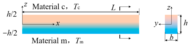
The coordinate definitions, material distribution, and dimensions of the beam are illustrated in Figure 1. L and h represent the beam length (x-direction) and thickness (z- direction), respectively. The model under consideration is an FG beam made of a mixture of material m (indicated by subscript “m”) and material c (indicated by subscript “c”).
The temperature dependence of material properties can be described by a nonlinear equation [22]:
S i = P 0 P 1 T 1 + 1 + P 1 T + P 2 T 2 + P 3 T 3
where S represents material properties such as elastic modulus E, density ρ , Poisson’s ratio ν , thermal expansion coefficient α and thermal conductivity k. The subscript i = c and m, represents material c and m, respectively. T represents temperature, P 0 , P 1 , P 1 , P 2 and P 3 are coefficients of temperature-dependent material properties, given by test.
According to the power-law assumption [23] and the rule of mixture [24], the effective material properties are as follows [22]:
S ( z , T ) = S m ( T ) + S c ( T ) S m ( T ) z h + 1 2 P z
where P z symbolize the power-law exponent.
When the ambient temperature increases or decreases uniformly, a uniform temperature field is established, and the temperature at any point within the beam can be expressed as follows [23]:
T e ( z ) = T even
where Te denotes the uniform temperature field and Teven denotes the prescribed temperature.
The linear temperature field, characterized by a linear temperature variation through the beam thickness, is commonly used in the absence of detailed thermal conductivity data or for modeling simplification [25]:
T l ( z ) = T m + ( T c T m ) z h + 1 2
where T1 denotes the linear temperature field and Tm and Tc denote the temperatures at the beam bottom and top surfaces, respectively.
When the top and bottom surfaces of the beam are subjected to different temperatures, a nonlinear one-dimensional steady-state temperature field is established through the thickness. In the absence of heat sources, the governing one-dimensional heat conduction equation is given by the following [26]:
d d z k ( z ) d T ( z ) d z = 0
The Dirichlet temperature boundary conditions on the top and bottom surfaces of the beam are given by the following [26]:
T ( h 2 ) = T m , T ( h 2 ) = T c
The temperature at any point within the beam is obtained by solving Equations (5) and (6):
T n ( z ) = T m + Δ T h / 2 z 1 k ( z ) d z h / 2 h / 2 1 k ( z ) d z
where Tn denotes the nonlinear temperature field. The temperature difference is defined as
Δ T = T c T m
According to Timoshenko beam theory, the axial displacement u and transverse displacement w at any point on the beam are as follows [19]:
u ( x , z , t ) = u 0 ( x , t ) + z φ ( x , t ) w ( x , z , t ) = w 0 ( x , t )
where u0(x, t) and w0(x, t) denote the displacements of the neutral layer (z = 0) of the beam along the x- and z-directions, respectively, φ (x, t) represents the rotation angle of this point about the y-axis, and t denotes time. Although the displacement field of the beam is related to the variables x, z, and t, for the sake of simplified expression, u0(x, t) is abbreviated as u, and other variables related to displacement and strain are simplified in the same manner.
According to the small deformation assumption, the normal strain and shear strain are given by the following [19]:
ε x x = u x , γ x z = u z + w x
When the effect of temperature variation is neglected, the stress–strain relationship satisfies the following [19]:
σ x x = E ( z ) 1 ν ( z ) 2 ε x x , σ x z = K s γ x z E ( z ) 2 1 + ν ( z )
where Ks denotes the shear correction coefficient dependent on the cross-sectional geometry.
The governing equations derived from the Timoshenko beam theory and Hamilton’s principle are as follows [19]:
A x x 2 u x 2 + B x x 2 φ x 2 I 0 2 u t 2 I 1 2 φ t 2 = 0 C x z 2 w x 2 + φ x N T 2 w x 2 I 0 2 w t 2 = 0 B x x 2 u x 2 + D x x 2 φ x 2 C x z w x + φ I 1 2 u t 2 I 2 2 φ t 2 = 0
where the cross-section stiffness-related coefficients are defined as follows [19]:
( A x x , B x x , D x x ) = h / 2 h / 2 E ( z ) ( 1 , z , z 2 ) d z C x z = K s h / 2 h / 2 G ( z ) d z
where G denotes shear modulus, defined as follows [19]:
G ( z ) = E ( z ) 2 ( 1 + ν ( z ) )
and the cross-section moment of inertia-related coefficients are defined as follows [19]:
( I 0 , I 1 , I 2 ) = h / 2 h / 2 ( 1 , z , z 2 ) ρ ( z ) d z
where N T denotes thermally induced force[19]:
N T z = h / 2 h / 2 E ( z ) 1 ν 2 ( z ) α ( z ) ( T i T 0 ) d z
where T0 denotes the reference temperature and T i denotes temperature of different temperature fields, the subscript i = e, l, n.

3. Results

The state-space method (SSM) is employed to solve the vibration governing equations. Rooted in control theory and finite element concepts [27], SSM offers high computational efficiency, excellent accuracy, and a unified framework for handling various boundary conditions [27,28,29].
According to the method of separation of variables [30], the solution to the governing Equation (12) can be expressed as
u = U ( x ) e i ω t w = W ( x ) e i ω t φ = ϕ ( x ) e i ω t
where ω denotes the natural angular frequency, while U ( x ) , W ( x ) and ϕ ( x ) represent the mode shape functions that satisfy the prescribed boundary conditions.
The following dimensionless quantities are introduced:
W ¯ = W L , ϕ ¯ = ϕ , U ¯ = U L , x ¯ = x L
Substituting Equations (17) and (18) into the governing Equation (12) and applying a simple mathematical transformation [31] yields
d 2 ϕ ¯ ( x ¯ ) d x ¯ 2 = C x z L 2 A 1 d W ¯ ( x ¯ ) d x ¯ B 1 L 3 A 1 U ¯ ( x ¯ ) C 1 L 2 A 1 ϕ ¯ ( x ¯ ) d 2 U ¯ ( x ¯ ) d x ¯ 2 = B x x C x z L D x x A 2 d W ¯ ( x ¯ ) d x ¯ B 2 L 2 A 2 U ¯ ( x ¯ ) C 2 L A 2 ϕ ¯ ( x ¯ ) d 2 W ¯ ( x ¯ ) d x ¯ 2 = C x z A 3 d ϕ ¯ ( x ¯ ) d x ¯ I 0 ω 2 L 2 A 3 W ¯ ( x ¯ )
where the coefficients are defined as
A 1 = D x x B x x 2 A x x , B 1 = I 1 ω 2 B x x I 0 ω 2 A x x , C 1 = I 2 ω 2 C x z B x x I 1 ω 2 A x x A 2 = A x x B x x 2 D x x , B 2 = I 0 ω 2 I 1 B x x D x x ω 2 , C 2 = I 1 ω 2 B x x I 2 ω 2 D x x B x x C x z D x x A 3 = C x z N T
According to SSM, the state vector is defined as
η ( x ¯ , ω ) = W ¯ ( x ¯ ) , d W ¯ ( x ¯ ) d x ¯ , U ¯ ( x ¯ ) , d U ¯ ( x ¯ ) d x ¯ , ϕ ¯ ( x ¯ ) , d ϕ ¯ ( x ¯ ) d x ¯ T
The governing Equation (19) is reformulated in state-space form by introducing the state vector, yielding
d η ( x ¯ , ω ) d x ¯ = Φ ( ω ) η ( x ¯ , ω )
where the coefficient matrix is defined as
Φ ( ω ) = 0 1 0 0 0 0 I 0 ω 2 L 2 A 3 0 0 0 0 C x z A 3 0 0 0 1 0 0 0 B x x C x z L D x x A 2 B 2 L 2 A 2 0 C 2 L A 2 0 0 0 0 0 0 1 0 C x z L 2 A 1 B 1 L 3 A 1 0 C 1 L 2 A 1 0
Integrating both sides of Equation (22), the solution can be expressed as
η ( x ¯ , ω ) = e Φ ( ω ) x ¯ η ( 0 , ω )
The boundary conditions can be uniformly expressed as
M ( ω ) η ( 0 , ω ) + N ( ω ) η ( 1 , ω ) = 0
where M ( ω ) and N ( ω ) denote the boundary condition selection matrices at the left ( x ¯ = 0 ) and right end ( x ¯ = 1 ) of the beam, respectively.
For clamped-clamped (CC) boundary conditions,
U ¯ ( 0 ) = 0 , W ¯ ( 0 ) = 0 , ϕ ¯ ( 0 ) = 0 U ¯ ( 1 ) = 0 , W ¯ ( 1 ) = 0 , ϕ ¯ ( 1 ) = 0
where the corresponding boundary condition selection matrices are
M ( ω ) = 1 0 0 0 0 0 0 0 0 0 0 0 0 0 1 0 0 0 0 0 0 0 0 0 0 0 0 0 1 0 0 0 0 0 0 0 ,   N ( ω ) = 0 0 0 0 0 0 1 0 0 0 0 0 0 0 0 0 0 0 0 0 1 0 0 0 0 0 0 0 0 0 0 0 0 0 1 0
For simple-simple (SS) boundary conditions,
u ( x , z ) = 0 , w ( x , z ) = 0 M y = B x x u x + D x x φ x = 0
where the boundary condition selection matrices are
M ( ω ) = 1 0 0 0 0 0 0 0 0 0 0 0 0 0 1 0 0 0 0 0 0 0 0 0 0 0 0 0 0 0 0 0 0 0 0 1 ,   N ( ω ) = 0 0 0 0 0 0 1 0 0 0 0 0 0 0 0 0 0 0 0 0 0 1 0 0 0 0 0 0 0 1 0 0 0 0 0 0
Substituting Equation (24) into Equation (25) yields
M ( ω ) + N ( ω ) e Φ ( ω ) η ( 0 , ω ) = 0
According to Equation (30), the non-zero solution for the state vector η ( 0 , ω ) exists if and only if
det M ( ω ) + N ( ω ) e Φ ( ω ) = 0
Solving the eigen Function (31) yields the natural frequencies ω n , where the subscript n denotes the n-th mode. The corresponding modal shape is given by
η ( x ¯ , ω n ) = e Φ ( ω n ) x ¯ η ( 0 , ω n )
For convenience in parametric analysis, the natural frequency is nondimensionalized as follows [32]:
ω ¯ n = ω n L 2 ρ c A E c I
where ρ c and Ec denote the density and elastic modulus of material c, respectively. A represents the beam cross-sectional area, and I represents the inertia moment of the cross-section.

4. Discussion

Experimental and theoretical validation is conducted to verify the accuracy and validity of the proposed theoretical model. In the experiments, the natural frequencies and mode shapes of an FG beam under a nonlinear temperature field are measured. For the theoretical comparison, the first three natural frequencies of the beam under nonlinear temperature fields are calculated, accounting for temperature-dependent material properties.

4.1. Validation

4.1.1. Experimental Validation

An experimental platform for free vibration testing of FG beams under thermal environments is established in this section. The natural frequencies of the beam under nonlinear temperature fields are measured, thereby validating the theoretical model.
The top surface of the tested beam is composed of aluminum nitride (AIN), and the bottom surface is molybdenum (Mo). The beam has a length L = 50 mm, width b = 4 mm, and thickness h = 2 mm, resulting in a slenderness ratio L/h = 25. The power-law index is Pz = 2. The beam is configured with SS boundary conditions, and the fixtures are machined from cast iron. The material properties of the two constituents are provided in Table 1.
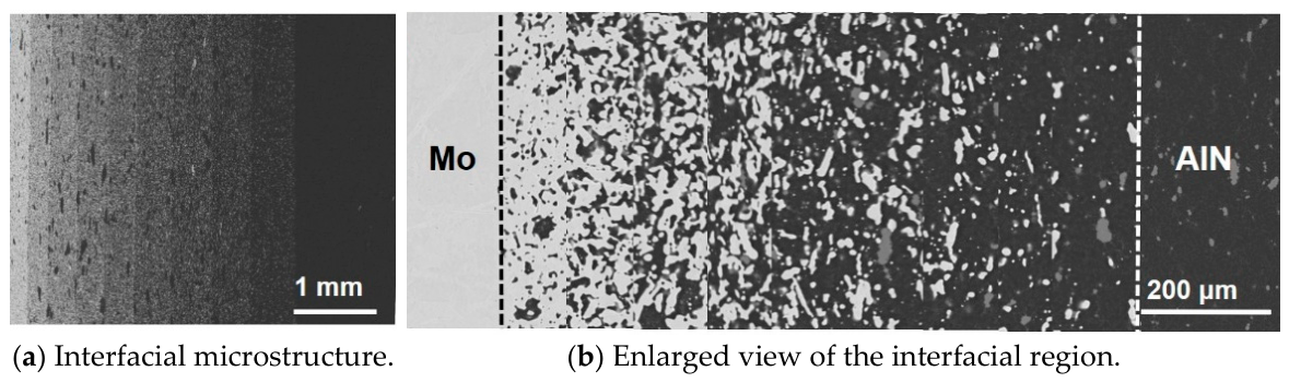
An FG beam is fabricated via hot-press sintering. The microstructure of the beam’s cross-section is characterized using scanning electron microscopy (SEM) and electron probe microanalysis (EPMA), as shown in Figure 2. Figure 2a presents the interfacial microstructure of the material under sintering conditions, revealing a graded transition zone consisting of nine layers. Figure 2b shows an enlarged view of the interface region in (a), where the microstructural morphology of the Mo-rich and AIN-rich transition layers can be more clearly identified. During the transition from the AIN ceramic layer to the Mo metal layer, as the Mo content gradually increases, the metallic phase (white regions) tends to agglomerate and progressively forms a continuous metal network, while the ceramic phase transforms from a continuous network into discretely distributed particles embedded within the metal matrix. In the graded layers with a Mo content exceeding 50%, both the metal and ceramic phases exhibit continuous interpenetrating network structures, mutually interlocked and nested, forming a three-dimensional interpenetrating composite architecture. The phase transition is smooth and gradual, in good agreement with the theoretical assumptions.
Next, a temperature control system capable of providing a thermo-vibration testing environment is designed to apply temperature boundary conditions to the aforementioned FG beam. The primary function of the system is to implement temperature boundary loading. When the temperatures of the top and bottom surfaces of the beam differ, a steady-state nonlinear temperature field within the beam is formed via heat conduction.
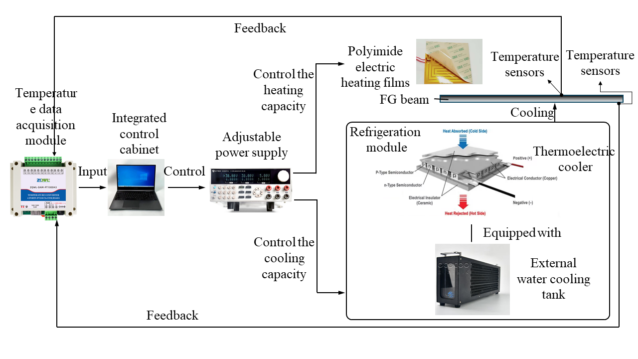
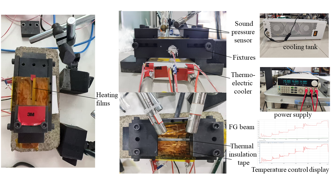
Accordingly, the designed temperature control system consists of a refrigeration module, an external water cooling tank, a heating module, a temperature acquisition module, temperature sensors, an integrated control cabinet, and control software. Specifically, the refrigeration module adopts a TEC1-25506 thermoelectric cooler (TEC Solutions Inc., Sunnyvale, CA, USA), equipped with a water cooling tank and water cooling module, enabling a maximum cooling temperature difference of 75 °C. The control module utilizes a TCM-type temperature control unit. The heating module employs polyimide electric heating films for heating, with a maximum achievable temperature of 180 °C. A ZQWL-DAM-PT100D43 (IVYTECH, Guangdong, China) data acquisition system is used to collect vibration signal data. An IV-3006T-3 (IVYTECH, Guangdong, China) programmable power supply with a 5-digit voltage and 4-digit current digital display adjusts the current based on feedback from the temperature sensors on the top and bottom surfaces of the beam, controlling the cooling and heating capacities in real time to ensure temperature stability of the beam surfaces and simulate a steady-state thermal environment after thermal equilibrium is achieved. The schematic of the temperature control system is illustrated in Figure 3.
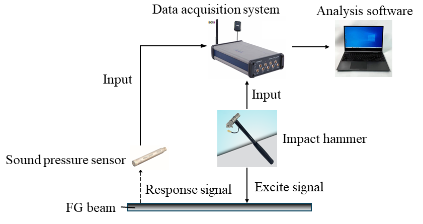
The natural frequencies of the beam are measured using an impact hammer testing method. The test system consists of an impact hammer, a sound pressure sensor, a data acquisition system, and analysis software. An NV9310 impact hammer ((NVIDIA, Santa Clara, CA, USA) is used to excite the beam and capture the input force signal, while the response signal is acquired using an MPA201 sound pressure sensor in a non-contact configuration. The excitation and response data are collected via an INV3062C dynamic signal acquisition system (COINV, Beijing, China). The data are then recorded and processed using DASP-V11 software (COINV, Beijing, China) for modal analysis. A schematic illustration of the vibration testing setup is shown in Figure 4.
The final experimental setup is illustrated in Figure 5.
Under a nonlinear temperature field, the top surface of the beam is heated using an electric heating pad, while the bottom surface is cooled by a thermoelectric cooler. The cooling power is real-time regulated based on temperature measurements from sensors to maintain a prescribed temperature difference Δ T . The first-order natural frequency ω 1 and mode shape of the beam are experimentally measured and compared with theoretical predictions, as presented in Table 2. Since many studies in the literature assume a constant Poisson’s ratio of ν = 0.3, this study also investigates the influence on ω 1 under two scenarios: (1) when the Poisson’s ratios of the upper and lower surface materials are different, and (2) when they are both set to 0.3. This comparison allows for an assessment of the validity of the commonly adopted simplification.
As shown in Table 2, with experimental values taken as reference, the relative error between theoretical and experimental results is very small—less than 1%. As the temperature difference increases, the theoretical ω 1 converge further toward the experimental values, primarily due to the softening of the heating pad at elevated temperatures, which improves its contact conformity with the beam surface and thereby reduces measurement uncertainty. The comparison confirms the correctness of the beam model under thermal environments and demonstrates the high computational accuracy of SSM. Many studies in the literature assume a constant Poisson’s ratio of ν = 0.3, or set νc = νm = 0.3 for simplicity. In the experimented AlN–Mo FG system, the constituent Poisson’s ratios are νc = 0.21 and νm = 0.35. When Pz = 2, the effective Poisson’s ratio ν(z) varies with z, but remains extremely close to 0.3 over the majority of the beam domain. Numerical comparisons reveal that the results obtained under the assumption ν = 0.3 deviate from those considering the spatial variation in ν(z) by less than 1 × 10 6 in relative error despite of temperature difference. This negligible discrepancy demonstrates that the simplified assumption of a constant ν = 0.3 is fully justified for practical modeling purposes in this case.
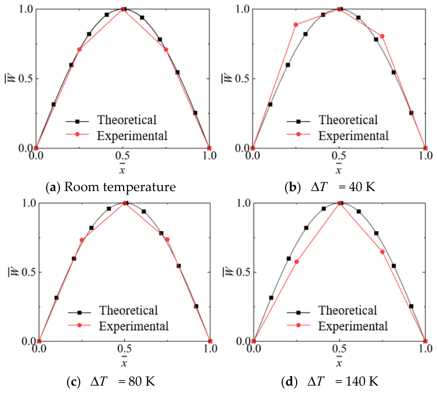
The theoretical and experimental mode shapes at room temperature and under Δ T of 40 K, 80 K, and 140 K are compared in Figure 6.
In the experiment, due to the small dimensions of the beam and the limited number of impact points, the obtained mode shape curves exhibit insufficient smoothness. However, the displacements at the measurement points closely align with the theoretical predictions. The overall trend and shape of the two curves match well, without significant distortion or deviation, indicating that the theoretical model is appropriately constructed and the solution approach is reliable.
To sum up, although differences between experimental and theoretical results arise due to various error sources—such as the small specimen size, non-isothermal conditions, non-contact measurement constraints, additional mass from the heating pad, lead wire effects, and ambient noise—the overall trends of the two sets of data are consistent. The relative error between the measured and calculated values remains below 1%, which effectively validates the correctness of the theoretical modeling and the high accuracy of the SSM adopted for the solution.

4.1.2. Theoretical Validation

The natural frequencies ω ¯ n of an FG Timoshenko beam under a linear temperature field are calculated with temperature-dependent material properties.
The top surface of the beam is composed of silicon nitride (Si3N4), and the bottom surface is stainless steel (SUS304). The temperature-dependent material properties are shown in Table 3. Unless otherwise stated, T0 = 300 K, Tm = 5 K + T0, L/h = 20. Ks = 5/6, Pz = 2, SS boundary condition.
The first three natural frequencies of the beam under a linear temperature field are calculated by varying Δ T and Pz. The results are compared with the Navier solution from Ref. [22], as summarized in Table 4.
It is evident that, when Δ T and Pz are varied, the first three ω ¯ n computed in this study show excellent agreement with those reported in the literature, confirming the correctness of the proposed beam model and demonstrating that the SSM is well-suited for solving the thermoelastic vibration equations of the beam, with high solution accuracy and reliability.

4.1.3. Multiple Boundary Conditions Validation

The natural frequencies ω ¯ 1 of beams under multiple boundary conditions are calculated and validated in this section.
The top surface of the beam is composed of Al2O3, and the bottom surface is Al. Unless otherwise stated, Ks = 5/6, Pz = 0.3, ω ¯ 1 = ω 1 L 2 / h h / 2 h / 2 ρ d z / h / 2 h / 2 E d z . The results are compared to the Lagrange multiplier method [33] and the Navier method [34].
It can be observed that ω ¯ 1 calculated by the SSM are in excellent agreement with those obtained by the analytical Navier method and the numerical Lagrange multiplier method under different slenderness ratios and boundary conditions. Furthermore, the Navier method is only applicable to simply supported boundary conditions, whereas the SSM adopted in this study is not restricted by this limitation and can accurately calculate ω ¯ 1 under various boundary conditions.

4.2. Parameter Study

The effects of uniform, linear, and nonlinear temperature distributions on frequency, mode shapes, and thermally induced forces are comparatively analyzed. Based on this, the coupled influence of the temperature field with the power-law index, slenderness ratio, and boundary conditions is further investigated.

4.2.1. Effects of the Temperature Field

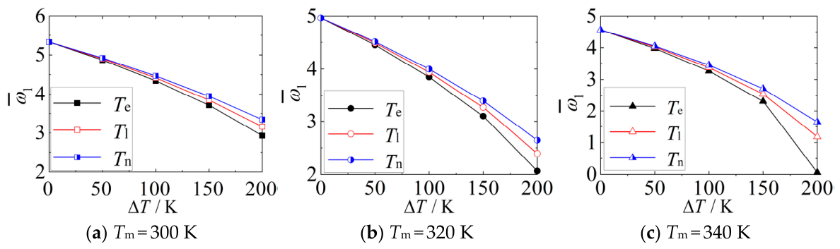
Temperature elevation reduces the natural frequency ω ¯ 1 of FG beams. The ω ¯ 1 variation curves differ under various temperature fields and distribution patterns. Therefore, the variation laws of ω ¯ 1 and the corresponding thermally induced forces NT are investigated in this section under uniform (Te), linear (Tl), and nonlinear temperature fields (Tn) by varying temperature difference Δ T . Pz = 2, L/h = 20, T0 = 300 K.
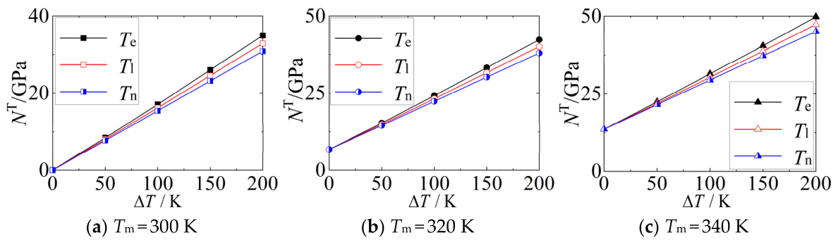
According to the expression of NT (Equation (16)), NT depends not only on structural parameters such as E, α, and ν , but also on the temperature field pattern, Tc and Tm, i.e., on the environmental temperature difference (TmT0) and temperature difference (TcTm). Hence, Figure 7 presents the variation in ω ¯ 1 with respect to Tc and Tm under uniform Te, linear Tl, and nonlinear temperature fields Tn. Figure 8 shows the corresponding variation in NT.
From Figure 7, under all three temperature fields, ω ¯ 1 decreases with increasing Δ T , and the overall trend is similar. As shown in the vibration governing Equation (12), NT affects only coefficient A3, which governs displacement along the beam’s height direction z. At relatively low temperatures, the magnitude of NT is smaller than the shear stiffness coefficient Cxz. Under all three temperature fields, A3 remains positive, with only its value changing, resulting in a similar mechanism by which NT influences ω ¯ 1 . Quantitatively, NT is smallest under the nonlinear temperature field and largest under the uniform field. As shown in Figure 7, ω ¯ 1 decreases slowest and remains highest under the nonlinear temperature field, whereas it is opposite for the uniform one, and the rate of ω ¯ 1 reduction increases with larger Δ T . The linear temperature field lies between the two, closer to the uniform case. As Δ T increases, NT increases linearly, with the fastest growth observed under the uniform field, the slowest under the nonlinear field, and intermediate behavior under the linear field. This phenomenon arises because the additional temperature field induces axial compressive stress due to thermal expansion, leading to a reduction in equivalent stiffness—known as the stress-softening effect—where a greater NT results in a lower ω ¯ 1 .
From Equations (3), (4), (7), and (16), NT depends not only on material properties but also on the ambient temperature difference and Δ T . Under the three temperature fields, the effect of ambient temperature difference on NT is identical. Therefore, in Figure 7 and Figure 8, when only Tm varies, the variation in ω ¯ 1 with Δ T follows a similar trend across all three temperature fields, and the corresponding NT curves exhibit the same slope (Figure 8). For different values of Tm, the NT curves shift vertically without changing shape. Physically, this occurs because, although the beam’s overall temperature increases or decreases, the form of the temperature distribution remains unchanged—only a vertical shift in the temperature profile is introduced.
To better analyze the influence of temperature-dependent material properties on ω ¯ 1 , Table 5, Table 6 and Table 7 compare the changes in ω ¯ 1 and t NT under two cases: one where material properties vary with temperature (temperature-dependent), and the other where they remain constant (temperature-independent).
Table 5. Comparison of ω ¯ 1 under multiple boundary conditions.
SSCC
L/hPresentRef. [34]Ref. [33]L/hPresentRef. [34]Ref. [33]
102.70182.70032.701105.8690-5.875
302.73812.73792.738306.1754-6.177
1002.74232.74232.7421006.2136-6.214
Table 6. Effects of temperature-dependent and temperature-independent material properties on ω ¯ 1 .
Temperature-DependentTemperature-IndependentRelative Change
Δ T /KTeTlTnTeTlTn
05.32795.32795.32795.32795.32795.32790.00%0.00%0.00%
504.86824.9014.91964.87214.89134.90580.08%−0.20%−0.28%
1004.33914.41484.46474.36914.41174.44380.69%−0.07%−0.47%
1503.71193.84693.94763.80013.87333.92792.38%0.69%−0.50%
2002.92563.1543.33963.12923.24663.3336.96%2.94%−0.20%
Table 7. Effects of temperature-dependent and temperature-independent material properties on NT.
Temperature-DependentTemperature-IndependentRelative Change
Δ T /KTeTlTnTeTlTn
00000000.00%0.00%0.00%
508.44548.05477.7328.33547.99987.745−1.30%−0.68%0.17%
10017.102516.22215.44316.670815.999615.49−2.52%−1.37%0.30%
15025.958724.50623.1425.006223.999423.235−3.67%−2.07%0.41%
20035.000532.90930.83133.341631.999130.98−4.74%−2.76%0.48%
In a uniform temperature field, the temperature-independent thermally induced force NT is smaller than that in the temperature-dependent case, leading to an increase in ω ¯ 1 . In a linear temperature field, when the temperature difference Δ T is small, the variation in material properties with temperature is negligible, and the effect of NT dominates. In this scenario, the NT under the temperature-independent case is small, which would theoretically result in a higher ω ¯ 1 . However, due to the combined effects of E, α, and ν, ω ¯ 1 remains almost unchanged, or even slightly lower than that in the case with temperature-dependent material properties. In a nonlinear temperature field, the temperature dependence of thermal conductivity k alters the temperature distribution, resulting in a lower NT in the case with temperature-dependent material properties compared to that with constant material properties. Consequently, ω ¯ 1 is higher when considering temperature-dependent material properties.
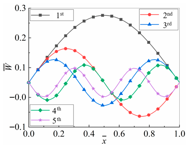
The mode shapes of the beam remain nearly unchanged when Tm, Δ T , and temperature field profile are varied. The first five mode shapes under a nonlinear temperature field with Tm = 320 K and Δ T = 100 K are shown in Figure 9, corresponding to the natural frequencies ω ¯ 1 = 3.9979, ω ¯ 2 = 19.9502, ω ¯ 3 = 45.4985, ω ¯ 4 = 79.6868, ω ¯ 5 = 121.2926, respectively.
From Figure 9, the first five mode shapes of the FG beam exhibit a similar form and variation pattern to those of a homogeneous beam. In the mode shape expression, temperature changes primarily affect the coefficient of the second-order derivative term of the transverse displacement function. In the governing equation, this corresponds to the first-order derivative term of the mode shape function, which has negligible influence on the mode shape itself. Consequently, the overall mode shape remains essentially unchanged under varying temperatures.
The results indicate that ω ¯ 1 decreases with increasing NT. Under a uniform temperature field, the beam experiences the maximum NT and thus the lowest ω ¯ 1 ; under a nonlinear temperature field, NT is minimal, resulting in the highest ω ¯ 1 ; the linear temperature field yields intermediate values. For a given temperature profile, varying the ambient temperature merely shifts the temperature distribution and NT curve vertically, without altering their shape or slope. The mode shapes are minimally affected by temperature, remaining nearly unchanged when the Tm, Δ T , or temperature field profile is varied.

4.2.2. Effects of the Power-Law Index

The influence of the power-law index Pz and temperature difference Δ T on the natural frequencies ω ¯ 1 and thermally induced forces NT of an FG beam under uniform (Te), linear (Tl), and nonlinear temperature fields (Tn) is investigated in this section.
Since the distribution form of the temperature field is solely determined by Δ T and is independent of Tm. Without loss of generality, Tm is assumed to be constant (Tm = T0 + 5 K), and the analysis focuses on the influence of Δ T .
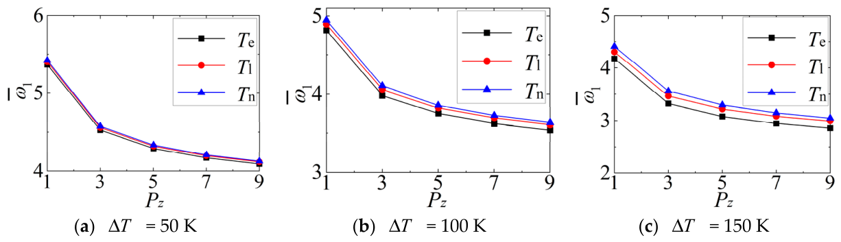
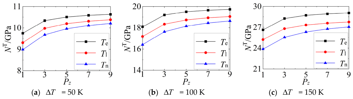
The effect of Pz and Δ T on ω ¯ 1 and NT under uniform, linear, and nonlinear temperature fields are shown in Figure 10 and Figure 11.
From Figure 10, under both uniform and nonlinear temperature fields, ω ¯ 1 decreases with increasing Pz, and the rate of decline diminishes as Pz increases. Correspondingly, NT increases with Pz, but the rate of increase gradually reduces (Figure 8). This behavior arises because Pz represents the volume fraction of the ceramic phase: when Pz = 0, the FG becomes pure ceramic, characterized by high E, low ρ , and high stiffness, resulting in higher ω ¯ 1 . As Pz increases, the metallic component gradually dominates, reducing the overall stiffness and consequently lowering ω ¯ 1 .
From Equation (16), NT relates to material properties of E, α , and ν , with E having the most significant influence. As Pz increases, NT also increases, but the rate of increase gradually decreases, a trend most pronounced under the nonlinear temperature field. Meanwhile, NT remains most stable under the uniform temperature field. According to Equations (3), (4), (7), and (16), NT can be decomposed into two components: one associated with the ambient temperature difference and the other with Δ T . When isolating material effects, the ambient temperature difference term is constant, while the Δ T term depends on the temperature field profile, yielding a constant NT under uniform conditions, a quadratic function of coordinate z under linear conditions, and a more complex expression under nonlinear conditions. This analytical result is confirmed in Figure 11: under the nonlinear temperature field, both temperature distribution and material parameters jointly influence NT and ω ¯ 1 , whereas under the uniform field, the force depends only on the material gradient. In the linear case, the trend of NT variation resembles that under uniform conditions, but its magnitude is closer to the nonlinear case. The mode shapes of the beam remain nearly unchanged when varying Pz.
At low Δ T , the ω ¯ 1 variation curves with respect to Pz are similar across all three temperature fields. As Δ T increases, the influence of Δ T and temperature field profile becomes more pronounced. ω ¯ 1 under the nonlinear temperature field decreasing most slowly and remaining the highest, accompanied by the smallest NT. In the uniform temperature field, the rate of ω ¯ 1 change with Pz remains constant when varying Δ T , resulting in nearly parallel curves. This is because, in the uniform case, the temperature distribution is independent of Pz; varying Pz only alters the magnitude of NT, which changes gradually (Figure 11) and is nearly proportional to Δ T , leading to parallel ω ¯ 1 trends. Similarly, in the linear temperature field, the distribution is also independent of Pz, so NT variation closely resembles that under uniform conditions. However, due to its magnitude being closer to the nonlinear case, the ω ¯ 1 response aligns more with the nonlinear field. Under the nonlinear temperature field, the rate of ω ¯ 1 decrease intensifies with increasing Δ T . Here, the temperature distribution depends on both Δ T and Pz, and Pz has a significant effect on ω ¯ 1 . As Δ T increases, NT rises rapidly—approaching the level observed under uniform conditions—resulting in an accelerated decline in ω ¯ 1 .
The above results indicate that the temperature-induced term, analogous to a stiffness coefficient, is added to the stiffness-relating tensile force and neutral-axis strain due to thermal effects, primarily influencing the transverse displacement in the governing equations, with its impact varying according to the magnitude of NT. Conclusions: (1) Under uniform, linear, and nonlinear temperature fields, NT increases with the Pz, but the growth rate gradually decreases; correspondingly, ω - 1 decreases as Pz increases, and the rate of decline diminishes with higher Pz. (2) At low Δ T , the ω - 1 variation curves with respect to Pz are similar across all three temperature fields; as Δ T increases, the influence of Δ T and the temperature field profile on ω - 1 becomes more pronounced. (3) ω - 1 under the nonlinear temperature field decreases most slowly, consistently remaining the highest, while NT remains the smallest; as Δ T increases, the rate of ω - 1 decrease intensifies. (4) The ω - 1 variation trend in the linear temperature field resembles that under the uniform field, but its magnitude is closer to the nonlinear case. (5) Under the uniform temperature field, the rate of ω - 1 change with Pz remains nearly constant when varying Δ T , resulting in nearly parallel curves.

4.2.3. Effects of the Slenderness Ratio

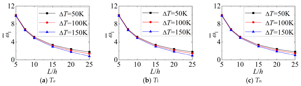
The influence of slenderness ratio and Δ T on ω ¯ 1 and NT under different temperature fields are investigated in this section. To eliminate dimensional effects, dimensionless parameters are defined as ω ¯ 1 = 1000 ω 1 L ρ c A / ( E c 0 I ) , where E c 0 denotes the elastic modulus of the top-surface material at Tc = 300 K. Figure 12 presents the variation in ω ¯ 1 with the slenderness ratio L/h under uniform (Te), linear (Tl), and nonlinear (Tn) temperature fields, with varying Δ T .
As shown in Figure 12, the variation in ω ¯ 1 with L/h is highly similar under the three temperature fields. ω ¯ 1 decrease as L/h increases, and the rate of decline diminishes at higher L/h. This is because, with constant h and increasing L, the beam’s equivalent E is reduced due to geometric changes, leading to a lower ω ¯ 1 .
As shown in Figure 12, at the same L/h, ω ¯ 1 under the linear temperature field is consistently the highest while that under the uniform temperature field is the lowest. The differences among the three ω ¯ 1 increase with rising Δ T . According to Equation (16), with identical Pz and L/h, NT primarily depends on the temperature distribution pattern, being maximum under uniform temperature field and minimum under nonlinear temperature field. This aligns with the conclusion in Section 4.2.1, indicating that, under a nonlinear temperature field, the beam’s NT is the lowest and its ω ¯ 1 is least affected by temperature variations.
Under the same Δ T , as L/h increases, the differences in ω ¯ 1 among the three temperature fields gradually enlarge. Although for a given Pz, NT, defined in Equations (3), (4), (7) and (16), remains constant under the same temperature field and Δ T —regardless of L/h—the influence of L/h extends beyond a single term in the equation. As shown in Equation (20), it is coupled with coefficients related to sectional stiffness, sectional mass moment of inertia, and the magnitude of NT. Therefore, ω ¯ 1 is primarily altered by the geometric configuration of the material.
The above results indicate that, under the three temperature fields, the variation in ω ¯ 1 with L/h is highly similar. The ω ¯ 1 decreases as L/h increases, and the differences in ω ¯ 1 grow larger with increasing L/h. Under the same temperature distribution pattern and identical Δ T , NT remains constant and is independent of L/h.

4.2.4. Effects of the Boundary Conditions

The influence of boundary conditions on ω ¯ 1 and NT is investigated under different temperature fields and Δ T .
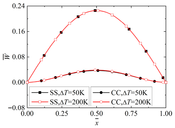
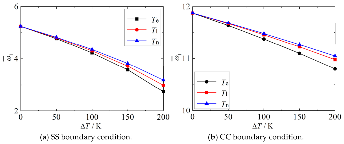
Figure 13 shows the variation of ω ¯ 1 under SS and CC boundary conditions with changing Δ T in uniform, linear, and nonlinear temperature fields. Figure 14 presents the corresponding mode shapes.
As shown in Figure 13, under both boundary conditions, ω ¯ 1 decreases with increasing Δ T . For a given boundary condition, ω ¯ 1 corresponding to the nonlinear temperature field is consistently the highest, while that under the uniform temperature field is the lowest, and ω ¯ 1 in the linear temperature field is closer to that under the nonlinear field—consistent with the conclusion in Section 4.2.1. Under the CC boundary condition, ω ¯ 1 exhibits an approximately linear decline with rising Δ T , whereas under the SS boundary condition, the rate of decrease increases with Δ T , particularly under the uniform temperature field where the decline is the most rapid.
As indicated in Figure 14, the mode shapes remain essentially unchanged with varying Δ T . With increasing Δ T , thermal expansion occurs in the structure. Under CC boundary conditions, the fixed supports constrain axial, shear, and bending deformations, resulting in smaller displacements and less sensitivity of ω ¯ 1 to temperature variations. In contrast, under SS boundary conditions, the absence of moment restraint allows for larger flexural deformation, leading to a reduction in equivalent stiffness and a more pronounced decrease in ω ¯ 1 as Δ T increases.
The above results demonstrate that under the CC boundary condition, ω ¯ 1 exhibits a more stable variation trend with increasing Δ T . In contrast, due to the absence of moment restraint, under the SS boundary condition, ω ¯ 1 displays a significantly higher sensitivity to changes in Δ T .

5. Conclusions

The thermal vibration governing equations for FG beams under uniform, linear, and nonlinear temperature fields are established based on Timoshenko beam theory. The SSM is employed to derive analytical expressions for natural frequencies and mode shapes. Model correctness and solution accuracy are verified through a comparison with the literature and experimental testing. Subsequently, the composite influence of temperature field with power-law index, slenderness ratio, and boundary conditions is analyzed, leading to the following conclusions:
(1)
Temperature-induced changes in frequency are attributed to modifications in both governing equation coefficients and material properties. With regard to the governing equation coefficients, a temperature-dependent term—analogous to a stiffness coefficient—is introduced into the stiffness relation between axial force and mid-plane strain due to thermal effects, primarily influencing the transverse displacement equation of the beam. The extent of this influence varies with the magnitude of thermally induced force. Changes in material properties simultaneously affect both thermally induced force and equation coefficients, with the specific form of variation differing across temperature fields. For instance, in a uniform temperature field, the elastic modulus depends only on the average temperature, whereas in linear and nonlinear temperature fields, it is governed by both the top and bottom surface temperatures. Moreover, the elastic modulus exhibits a more pronounced reduction at higher temperatures.
(2)
Thermally induced force characterizes the extent to which temperature variation affects frequency. It is primarily altered by temperature-dependent material properties and the form of temperature distribution. Comparing uniform, linear, and nonlinear temperature fields, the thermally induced force decreases progressively, while the corresponding frequency increases. Furthermore, frequency decreases with increasing power-law index and slenderness ratio. Under clamped-clamped boundary conditions, frequency varies more steadily with temperature difference; in contrast, under simply supported boundary conditions, frequency exhibits greater sensitivity to changes in temperature difference.
(3)
The mode shapes of FG beams are nearly independent of temperature variations. In the mode shape expression, temperature changes primarily affect the coefficient of the second-order derivative term of the transverse displacement function. In the governing equation, this corresponds to the first-order derivative term of the mode shape function, which has negligible influence on the mode shape itself. Consequently, the overall mode shape remains essentially unchanged under varying temperatures. The beam’s mode shape curves exhibit minimal variation when the bottom surface temperature, temperature difference, and temperature field pattern are altered.

Author Contributions

Conceptualization, D.Y.; Data curation, C.C. and D.Y.; Formal analysis, C.C.; Investigation, C.C.; Methodology, C.C. and D.Y.; Project administration, X.Y., D.Y. and C.Z.; Resources, X.Y. and D.Y.; Software, B.L.; Supervision, C.Z. and B.L.; Validation, C.C. and X.Y.; Writing—original draft, C.C.; Writing—review and editing, X.Y., C.Z. and B.L. All authors have read and agreed to the published version of the manuscript.

Funding

This research was funded by Natural Science Foundation of Sichuan Province of China, grant number 2026NSFSC1241 and 2026NSFSC1243, and Doctoral Innovation Capacity Enhancement Program, grant number 25CAFUC04023.

Data Availability Statement

Some or all data, models, or code that support the findings of this study are available from the corresponding author upon reasonable request.

Conflicts of Interest

The authors declare no conflicts of interest.

References

  1. Niino, M.; Hirai, T.; Watanabe, R. Functionally gradient materials in pursuit of super heat resisting materials for spacecraft. J. Jpn. Soc. Compos. Mater. 1987, 13, 257–264. [Google Scholar] [CrossRef] [Scilit]
  2. Koizumi, M. FGM activities in Japan. Compos. Part B Eng. 1997, 28, 1–4. [Google Scholar] [CrossRef] [Scilit]
  3. Bhavar, V.; Kattire, P.; Thakare, S.; Patil, S.; Singh, R.K.P. A review on functionally gradient materials (FGMs) and their applications. IOP Conf. Ser. Mater. Sci. Eng. 2017, 229, 012021.1–012021.10. [Google Scholar] [CrossRef] [Scilit]
  4. Boggarapu, V.; Gujjala, R.; Ojha, S.; Acharya, S.; Venkateswara Babu, P.; Chowdary, S.; Kumar Gara, D. State of the art in functionally graded materials. Compos. Struct. 2021, 262, 113596. [Google Scholar] [CrossRef] [Scilit]
  5. Zanoosi, A.A.P. Size-dependent thermo-mechanical free vibration analysis of functionally graded porous microbeams based on modified strain gradient theory. J. Braz. Soc. Mech. Sci. Eng. 2020, 42, 236. [Google Scholar] [CrossRef] [Scilit]
  6. Yang, X.; Liu, H.; Ma, J. Thermo-mechanical vibration of FG curved nanobeam containing porosities and reinforced by graphene platelets. Microsyst. Technol. 2020, 26, 2535–2551. [Google Scholar] [CrossRef] [Scilit]
  7. Ahmed, M.W.A.; Ahmad, R.N. Forced vibration analysis of functionally graded nanobeams via Complementary Functions Method in the Laplace domain. Thin-Walled Struct. 2026, 226, 114946. [Google Scholar] [CrossRef] [Scilit]
  8. Alhasan, A.M.W.; Noori, A.R. Free vibration analysis of functionally graded nanobeams via complementary functions method in the laplace domain. Arch. Appl. Mech. 2026, 96, 47. [Google Scholar] [CrossRef] [Scilit]
  9. Qais, G.; Mohammed, A.A.-O.; Muhammad, T.S.; Bourada, F.; Tounsi, A. Stability analysis of graphene-reinforced functionally graded plates on elastic foundations under different in-plane loads. Results Eng. 2026, 29, 109730. [Google Scholar] [CrossRef] [Scilit]
  10. Lakhdar, K.; Sadoun, M.; Addou, F.Y.; Bourada, F.; Bousahla, A.A.; Khedher, K.M.; Tounsi, A. Free vibrational characteristics of various imperfect FG beam via a novel integral Timoshenko’s theory. Acta Mech. 2024, 235, 6287–6304. [Google Scholar] [CrossRef] [Scilit]
  11. Gawah, Q.; Abdullah, M.A.; Al-Osta, M.A.; Bourada, F.; Tounsi, A.; Tounsi, A.; Yaylaci, M. Free vibration analysis of nonlinearly dispersed FG-CNTRC beams on Kerr substrate using an improved FSDT. Struct. Eng. Mech. 2025, 93, 475–493. [Google Scholar] [CrossRef]
  12. Abdeldjebbar, T.; Zakaria, B.; Fatima, B.; Balubaid, M.; Mahmoud, S.R.; Bousahla, A.A.; Tounsi, A. A Finite Element Approach for Forced Dynamical Responses of Porous FG Nanocomposite Beams Resting on Viscoelastic Foundations. Int. J. Struct. Stab. Dyn. 2026, 26, 2650078. [Google Scholar] [CrossRef] [Scilit]
  13. Abdelkader, S.; Abdelrahmane, B.B.; Mohammed, B.; Mahmoud, S.R.; Aljedani, J.; Algarni, A.; Ramady, A.; Meftah, S.A.; Tounsi, A. Instability of Porous FGM Rectangular Hollow Section (RHS) Beam Element in a Thermal Environment. Int. J. Struct. Stab. Dyn. 2026, 26, 2650065. [Google Scholar] [CrossRef] [Scilit]
  14. Wattanasakulpong, N.; Prusty, B.G.; Kelly, D.W. Thermal buckling and elastic vibration of third-order shear deformable functionally graded beams. Int. J. Mech. Sci. 2011, 53, 734–743. [Google Scholar] [CrossRef] [Scilit]
  15. Ebrahimi, F.; Hashemi, M. Vibration analysis of non-uniform imperfect functionally graded beams with porosities in thermal environment. J. Mech. 2017, 33, 739–757. [Google Scholar] [CrossRef] [Scilit]
  16. Akbaş, Ş.D. Thermal effects on the vibration of functionally graded deep beams with porosity. Int. J. Appl. Mech. 2017, 9, 1750076. [Google Scholar] [CrossRef] [Scilit]
  17. Ebrahimi, F.; Ghasemi, F.; Salari, E. Investigating thermal effects on vibration behavior of temperature-dependent compositionally graded Euler beams with porosities. Meccanica 2016, 51, 223–249. [Google Scholar] [CrossRef] [Scilit]
  18. Ebrahimi, F.; Salari, E. Nonlocal thermo-mechanical vibration analysis of functionally graded nanobeams in thermal environment. Acta Astronaut. 2015, 113, 29–50. [Google Scholar] [CrossRef] [Scilit]
  19. Ebrahimi, F.; Jafari, A. Thermo-mechanical vibration analysis of temperature-dependent porous FG beams based on Timoshenko beam theory. Struct. Eng. Mech. 2016, 59, 343–371. [Google Scholar] [CrossRef] [Scilit]
  20. Zahedinejad, P. Free vibration analysis of functionally graded beams resting on elastic foundation in thermal environment. Int. J. Struct. Stab. Dyn. 2016, 16, 1550029. [Google Scholar] [CrossRef] [Scilit]
  21. Shabanlou, G.; Hosseini, S.A.A.; Zamanian, M. Vibration analysis of FG spinning beam using higher-order shear deformation beam theory in thermal environment. Appl. Math. Model. 2018, 56, 325–341. [Google Scholar] [CrossRef] [Scilit]
  22. Ebrahimi, F.; Salari, E. Thermal buckling and free vibration analysis of size dependent Timoshenko FG nanobeams in thermal environments. Compos. Struct. 2015, 128, 363–380. [Google Scholar] [CrossRef] [Scilit]
  23. Swaminathan, K.; Sangeetha, D.M. Thermal analysis of FGM plates–A critical review of various modeling techniques and solution methods. Compos. Struct. 2017, 160, 43–60. [Google Scholar] [CrossRef] [Scilit]
  24. Kim, Y.W. Temperature dependent vibration analysis of functionally graded rectangular plates. J. Sound Vib. 2005, 284, 531–549. [Google Scholar] [CrossRef] [Scilit]
  25. Lal, R.; Dangi, C. Thermomechanical vibration of bi-directional functionally graded non-uniform timoshenko nanobeam using nonlocal elasticity theory. Compos. Part B Eng. 2019, 172, 724–742. [Google Scholar] [CrossRef] [Scilit]
  26. Yang, B.; Yang, J.; Kitipornchai, S. Thermoelastic analysis of functionally graded graphene reinforced rectangular plates based on 3D elasticity. Meccanica 2017, 52, 2275–2292. [Google Scholar] [CrossRef] [Scilit]
  27. Lei, Y.; Adhikari, S.; Friswell, M.I. Vibration of nonlocal Kelvin–Voigt viscoelastic damped Timoshenko beams. Int. J. Eng. Sci. 2013, 66, 1–13. [Google Scholar] [CrossRef] [Scilit]
  28. Shen, Z.-B.; Jiang, R.-W.; Zhang, L.; Tang, G.-J. Nonlocal galerkin strip transfer function method for vibration of double-layered graphene mass sensor. Acta Mech. Solida Sin. 2018, 31, 94–107. [Google Scholar] [CrossRef] [Scilit]
  29. Shen, Z.-B.; Jiang, R.-W.; Zhang, D.-P. Thermal effect on vibration responses of double-layered graphene sheet–based nanomechanical resonators based on Galerkin strip transfer function method. Braz. J. Phys. 2019, 49, 667–677. [Google Scholar] [CrossRef] [Scilit]
  30. Kitipornchai, S.; Chen, D.; Yang, J. Free vibration and elastic buckling of functionally graded porous beams reinforced by graphene platelets. Mater. Des. 2017, 116, 656–665. [Google Scholar] [CrossRef] [Scilit]
  31. Chen, C.; Li, D.K.; Zhou, X.; Zhou, L.L. Thermal vibration analysis of functionally graded graphene platelets-reinforced porous beams using the transfer function method. Eng. Struct. 2023, 284, 115963. [Google Scholar] [CrossRef] [Scilit]
  32. Ebrahimi, F.; Salari, E. Effect of various thermal loadings on buckling and vibrational characteristics of nonlocal temperature-dependent functionally graded nanobeams. Mech. Adv. Mater. Struct. 2016, 23, 1379–1397. [Google Scholar] [CrossRef] [Scilit]
  33. Şimşek, M. Fundamental frequency analysis of functionally graded beams by using different higher-order beam theories. Nucl. Eng. Des. 2010, 240, 697–705. [Google Scholar] [CrossRef] [Scilit]
  34. Wang, Y.; Xie, K.; Fu, T.; Shi, C. Vibration response of a functionally graded graphene nanoplatelet reinforced composite beam under two successive moving masses. Compos. Struct. 2019, 209, 928–939. [Google Scholar] [CrossRef] [Scilit]
Figure 1. Coordinate definition and dimensions of the FG beam.
Jcs 10 00272 g001
Figure 2. Microstructure of the FG beam cross-section.
Jcs 10 00272 g002
Figure 3. Schematic diagram of the temperature control system.
Jcs 10 00272 g003
Figure 4. Schematic diagram of the vibration testing setup.
Jcs 10 00272 g004
Figure 5. Experimental setup for beam vibration test under thermal conditions.
Jcs 10 00272 g005
Figure 6. Comparison of theoretical and experimental mode shapes.
Jcs 10 00272 g006
Figure 7. Effects of Tm and Δ T on ω ¯ 1 .
Jcs 10 00272 g007
Figure 8. Effects of Tm and Δ T on NT.
Jcs 10 00272 g008
Figure 9. The first five mode shapes of an FG beam.
Jcs 10 00272 g009
Figure 10. Effects of Pz and Δ T on ω ¯ 1 .
Jcs 10 00272 g010
Figure 11. Effects of Pz and Δ T on NT.
Jcs 10 00272 g011
Figure 12. Effects of L/h and Δ T on ω ¯ 1 .
Jcs 10 00272 g012
Figure 13. Effects of boundary conditions and Δ T on ω ¯ 1 .
Jcs 10 00272 g013
Figure 14. Effects of boundary conditions and Δ T on mode shapes.
Jcs 10 00272 g014
Table 1. Material properties in the experiment.
MaterialMaterial PropertiesValue
AINEc/Pa300 × 109
ρ c /kg/m33260
ν c 0.21
α c /K−14.5 × 10−6
kc/W/m·K170
MoEm/Pa329 × 109
ρ m /kg/m310,220
ν m 0.35
α m /K−14.8 × 10−6
km/W/m·K138
Table 2. Experimental and theoretical comparison of ω 1 for FG beams under nonlinear temperature fields.
ΔT/KTc/KTm/KTheoretical Values/HzTheoretical Values (v = 0.3)/HzExperimental Values/HzRelative Error/%
03003002695.542695.562689.140.24%
20312.15291.152688.242688.262667.50.78%
40331.15291.152644.512644.522634.380.38%
60351.15291.152597.682597.692578.130.76%
80372.15292.152545.142545.162539.630.22%
100393.15293.152491.502491.512497.71−0.25%
120415.15295.152431.602431.622437.25−0.23%
140436.15296.152375.402375.412381.95−0.27%
160459.15299.152307.152307.172313.28−0.26%
Table 3. Coefficients of temperature-dependent material properties [22].
MaterialPropertiesP0P−1P1P2P3
Si3N4Ec/Pa348.43 × 1090−3.07 × 10−42.16 × 10−7−8.946 × 10⁻¹¹
α c /K−15.8723 × 10−609.095 × 10−400
ρ c /kg/m323700000
ν c 0.240000
kc/W/m·K13.7230−1.032 × 10−35.466 × 10−7−7.876 × 10⁻¹¹
SUS304Em/Pa201.04 × 10903.079 × 10−4−6.534 × 10−70
α m /K−112.33 × 10−608.086 × 10−400
ρ m /kg/m381660000
ν m 0.32620−2.002 × 10−43.797 × 10−70
km/W/m·K15.3790−1.264 × 10−32.092 × 10−6−7.223 × 10⁻¹⁰
Table 4. Comparison of first three frequencies ω ¯ n with Ref. [22].
ω ¯ n Δ T = 10   K Δ T = 30   K Δ T = 60   K
PzPresentRef. [22]PzPresentRef. [22]PzPresentRef. [22]
ω ¯ 1 09.64629.646109.45399.453809.14759.1475
0.27.79647.79640.27.62117.62110.27.34207.3420
15.77175.771715.61045.610515.35365.3537
54.69254.692554.53634.536354.28754.2875
ω ¯ 2 038.668838.6688038.479438.4794038.183838.1838
0.231.321131.32220.231.156731.15790.230.900530.9016
123.287523.2890123.147723.1492122.930422.9319
518.999419.0001518.868618.8693518.666518.6672
ω ¯ 3 085.581685.5816085.391185.3911085.094685.0946
0.269.327269.33320.269.174169.18010.268.935368.9412
151.570351.5787151.457651.4659151.281051.2893
542.079842.0838541.981541.9855541.828241.8321
Disclaimer/Publisher’s Note: The statements, opinions and data contained in all publications are solely those of the individual author(s) and contributor(s) and not of MDPI and/or the editor(s). MDPI and/or the editor(s) disclaim responsibility for any injury to people or property resulting from any ideas, methods, instructions or products referred to in the content.