Reinventing the Trochoidal Toolpath Pattern by Adaptive Rounding Radius Loop Adjustments for Precision and Performance in End Milling Operations

Abstract

The present work intends to assess the impact of trochoidal toolpath rounding radius loop adjustments on surface roughness, nose radius wear, and resultant cutting force during end milling of AISI D3 steel. Twenty experimental trials have been performed utilizing a face-centered central composite design through a response surface approach. Artificial Neural Network (ANN) models were built to forecast outcomes, utilizing four distinct learning algorithms: the Batch Back Propagation Algorithm (BBP), Quick Propagation Algorithm (QP), Incremental Back Propagation Algorithm (IBP), and Levenberg–Marquardt Back Propagation Algorithm (LMBP). The efficacy of these models was evaluated using RMSE, revealing that the LMBP model yielded the lowest RMSE for surface roughness (Ra), nose radius wear, and resultant cutting force, hence demonstrating superior predictive capability within the trained dataset. Additionally, a Genetic Algorithm (GA) was employed to ascertain the optimal machining settings, revealing that the ideal parameters include a cutting speed of 85 m/min, a feed rate of 0.07 mm/tooth, and a rounding radius of 7 mm. Moreover, the detachment of the coating layer resulted in alterations to the tooltip cutting edge on the machined surface as the circular loop distance increased. The initial arc radius fluctuated by 33.82% owing to tooltip defects that alter the edge micro-geometry of machining. The measured and expected values of the surface roughness, resultant cutting force, and nose radius wear exhibited discrepancies of 6.49%, 4.26%, and 4.1%, respectively. The morphologies of the machined surfaces exhibited scratches along with laces, and side flow markings. The back surface of the chip structure appears rough and jagged due to the shearing action.

1. Introduction

The machined surfaces experience reduced tool life and compromised surface quality because of chipped edges, micro damages, flank wear, and surface defects at cutting tool tips [1]. Literature has investigated both the impact of cutting tool tip geometry and edge flutes along with the cutting speed and feed rate influencing the workpiece surface finishes [2]. Many different manufacturing sectors rely on end milling to produce die and mold components as well as functional items among others. Different tool path strategies, including linear and nonlinear, guide the end milling of these components [3]. The simultaneous execution of tool movements between circular and linear paths proves trochoidal milling as an exciting tool path strategy [4]. The industry widely deploys this method for manufacturing complicated cavities during end milling operations. Machines that operate at maximum efficiency require trochoidal milling because of its ability to handle complex geometries.

The analysis of trochoidal milling focused primarily on its benefits regarding machining time, cutting force, and tool life, yet researchers performed fewer studies about how parameters in trochoidal tool paths affect uncut chip thickness calculation and cutting force measurements [5]. According to Rong Yan et al. [6], employing trochoidal milling for narrow grooves production with large step size increases cutting forces along with undesired machine vibration which wears down the cutting tools. The optimized trochoidal toolpath described by Wu Shixiong et al. [7] works to shorten trajectory length when industrial process parameters within specified ranges are increased for trochoidal step size and feed rate and DOC and other settings, thereby enhancing the machining performance. Uhlmann et al. [8] examined the trochoidal machining effect on both the energy utilization and MRR during the cutting process of Ti-6Al-4V alloy. Research showed that raising effective energy consumption by 6% would result in at least a 35% cut in processing time through trochoidal milling practices. Research by Pleta et al. [9,10] proves that trochoidal milling generates higher productivity outcomes than traditional milling methods do. The authors of [11] introduced double trochoidal milling technology to advance trochoidal milling process efficiency. The trochoidal milling method created a 50.4% decrease in the overall cycle time needed for machining operations. The evidence showed that double trochoidal milling helped reduce cycle time, yet this approach generated tool wear alongside high cutting forces and produced severe chatter behavior at the tool path end due to abrupt direction changes.

The team of researchers led by Isuamfon F. Edem [12] examined how machine tool marginal setup combinations and tool movement patterns affect cutting operations’ electrical power consumption. The effect of sustainability in machining tool paths depends on the number of times a tool needs to retract during execution. The required electric energy for the machining process increases because of those tool retractions which extend the machining time duration. The proposed strategy for improved energy efficiency selects the tool path method that requires minimal tool retractions. Zeroudi et al. [13] created prediction mathematical models and geometrical representations to transform cutting force measurements from CL points which aid in developing tool paths during work piece processing. The results created fundamental possibilities for integrating CAM and analysis tools. This developed model enables analysis of the effect that cutting force level will present. The process control of hard material machining encounters difficulties when seeking desired quality characteristics. Testing different input parameters with trial-and-error methods used to be the traditional method for reaching desired quality characteristics. The release of these input parameters demanded substantial time duration. The total expenditure for the process increased substantially as well. The end milling process requires a new prediction method for quality characterization that minimizes time expenses and production costs. The manufacturing industry depends on ANN modeling to predict with greater accuracy than traditional approaches in the present era. The neural network program known as ANN emulates human brain functionality to predict output results from supplied input stimuli. Researchers have conducted numerous studies about output prediction by implementing ANN in manufacturing processes.

The research on ANN modeling for flat-end milling was developed by Topal and Palanisamy in their work [14,15]. The backpropagation algorithm delivered improved predictions according to their research findings. In his research work, Mohammed Mia used ANN and responses surface methodology to predict Ra and cutting force while milling Ti-6Al-4V [16]. The ANN model development occurred through MATLAB (R2016b 9.1) as the software platform. Sathiya et al., in their studies [17,18], demonstrated that the Neural Power Professional platform provides an easy way to demonstrate ANN and GA for accurate prediction and optimization results generation. The experimental process of Ra prediction using ANN approaches was performed by Pimenov et al. [19] and Quintana et al. [20] through MATLAB tool implementation after the milling operation. This modeling technique proves how CNC machines from recent times can estimate roughness deviation.

The use of Magnesium Alloys for AZ31 and AZ 91D during trochoidal toolpath machining was simulated through ANN. Statistica provides two ANN models (known as Radial Basis and Multi-layered Function) to serve effectively as predictive tools for milling force measurements and vibration tracking [21]. A range of ANN serves for predicting the Ra values at different stages of the Al alloy 7075-T7351 face milling machining process. Ra exhibited a strong correlation with chip thickness as well as cutting speed according to the study [22].

The research works of [23,24] presented an ANN model for Ra estimation in milling operations which incorporated ANN together with GA as the essential method for Ra measurement. The application of GA optimization resulted in a 12% increase in Ra while the process time experienced a 20% decrease when compared with initial cutting parameters. A Genetic Algorithm technique was applied as a concept to optimize process parameters that minimize Ra during end milling operations. The GA approach led to reduced Ra values, which decreased the experimental, Ra, and regression modeling results by 27%, 26%, and 50%, respectively [25].

Research investigations established that Ra acts as an essential quality indicator for part performance evaluations in applications related to aircraft and die and mold manufacturing. The temperature directly influences the deterioration of tools during operation. Scientists define specific cutting energy as the amount of cutting power needed to remove 1 mm³ of material but it is an essential factor for sustainability studies [26].

The literature review revealed the following procedural research gaps and motivation when using trochoidal tool paths to end mill AISI D3 steel. Research investigations have established that surface roughness (Ra) plays a significant role in determining performance, with a particular focus on aerospace and die/mold areas. However, how a toolpath geometry affects machining responses is not well understood, particularly for difficult to cut materials like the AISI D3 steel. Current studies are intended to solve this by enabling adaptive tool path approaches, but no study explores the correlation between trochoidal rounding radius loop adjustments and subsequent variations in the values of the surface integrity, cutting force, and tool nose wear. Moreover, the effect of changing the rounding radius on chip shape and tool interaction dynamics has not been investigated. This would uncover a necessity for methods that could predict and optimize interactions in high-performance machining applications. Consequently, the rounding radius loop is included as an innovative input parameter in this research and closes the knowledge gaps that exist by using Artificial Neural Network (ANN) models and optimization using a Genetic Algorithm (GA). This work is motivated by the necessity in industry to control surface finish and tool endurance in sophisticated materials, a need that the integrated ANN-GA approach is intended to solve by enabling adaptive tool path approaches based on data analysis.

The underlying innovation in this study is the incorporation and application of rounding radius loop control in the context of trochoidal toolpath strategies. Although much effort has been put into trochoidal milling analysis in terms of step size, toolpath length, and feed strategies, no previous studies have focused on how changes in the trochoidal rounding radius loop under CAM trajectory design influence the major machining results such as the surface roughness, cutting force, and tool nose wear. This work not only introduces this new parameter to the experimental method, but it also shows its importance through the ANN modeling and optimization using the genetic algorithms. The use of rounding radius as a flexible variable represents an important step up in the area and allows new adaptive approaches for the optimization of machining hard material, such as AISI D3 steel. An analysis of the chip morphology was conducted to study how the rounding radius loop in trochoidal paths impacts the formation process, which is not addressed in the literature.

2. Experimental Setup

2.1. Material Selection

The investigation employed AISI D3 steel that underwent the cold-working process. The selection of AISI D3 steel is strategically justified based on its widespread industrial application and challenging machinability characteristics. AISI D3 is a high carbon–high chromium cold—work tool steel that is distinguishable by its excellent wear resistance, dimensional stability, and hardness and is being widely used for manufacturing dies, molds, and cutting tools. Machining AISI D3 steel increases complexity due to its high hardness, 30–35 HRC, and low thermal conductivity, 20 W/mK, and often leads to rapid failure of the tool and surface damage. This investigation involves weight percent chemical analysis of the steel as presented in

Table 1. Chemical analysis of AISI D3.

Element	Vanadium (V)	Silicon (Si)	Chromium (Cr)	Manganese (Mn)	Carbon (C)	Nickel (Ni)	Iron (Fe)
Presence (wt. %)	0.25	0.3	11.5	0.4	2.1	0.31	Balance

while

Table 2. Mechanical properties of selected steel.

Workpiece Materials	Hardness, (HRC)	Tensile Strength, (N/mm2)	Density, (kg/cm3)	Yield Strength, (N/mm2)	Heat Conductivity, (W/mK)
AISI D3	30–35	970	7.7	850	20

displays the mechanical material properties.

2.2. Experimental Details

The end milling operation took place on a 3-axis VMC-BFW Gaurav machine that uses a Sinumerik 828D Siemens basic controller (Siemens AG, Munich, Germany). The machine’s workspace has dimensions of 450 mm × 350 mm × 350 mm due to the positioning of the modules across the x-axis, y-axis, and z-axis. The machine includes an 8000-rpm spindle speed together with a 10,000 mm/min feed rate and 3 KW of spindle motor power. This machine possesses a positioning precision measurement of ±0.005 mm accompanied by a repeatability accuracy of ±0.003 mm. The experiments took place in a dry-cutting environment under conditions of a 200 mm long and 50 × 50 mm cross-sectional slot. This research used the conditions stated in

Table 3. Parameters and their levels.

Factors	Level
	(−1)	(0)	(+1)
A. Cutting speed, (m/min)	50	70	90
B. Feed rate, (mm/tooth)	0.05	0.1	0.15
C. Rounding radius, (mm)	6	9	12

to perform AISI D3 steel machining operations.

Sandvik Coromant (ANSI R390-11 T3 08M-PM) tungsten carbide inserts with Ø12 mm size and 0.8 mm corner nose radius coated with solid titanium carbo-nitride were used as a cutting tool in the study. An R390-012A16-11L ISO-specified tool holder was used to hold the tool onto the machine. The BT40 adapter functioned as the tool-holding mechanism. The trochoidal milling process involved forward motion and uninterrupted loop circles to mill the cutting tool’s progressive paths. The trochoidal machining functionality within Mastercam X6 software was used to generate a simulated tool path displayed in Figure 1.

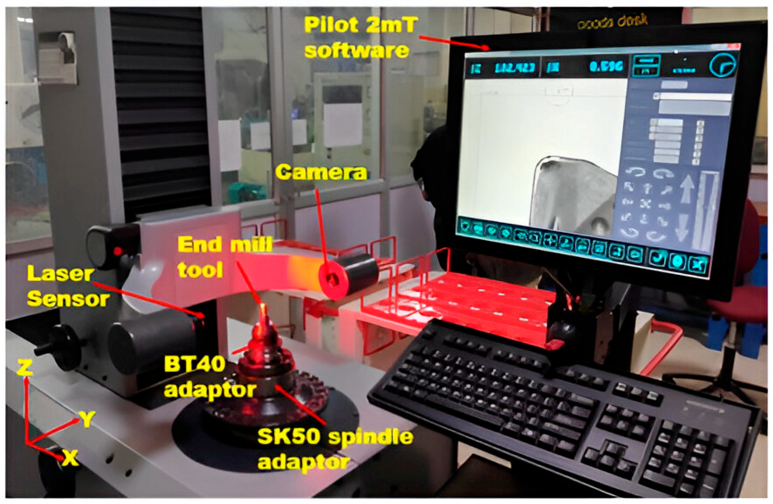
The trochoidal pitch distance takes its value from the tool diameter. Path pitch values were selected for tool safety at 50% of the diameter, and the rounding radius loop adjustment calculation depended on the CAM program’s cavity specifications. Machine operation for the narrow slot utilized a cavity section with dimensions 200 mm × 40 mm and DOC at 1 mm for each pass. Figure 2 shows the hardware arrangement and calibration equipment used throughout the research work.

2.3. Measurement of Output Responses

The Japan-made Surfcom 1400 G roughness tester from ACCRETECH (Tokyo Seimitsu Co., Ltd., Tokyo, Japan) operated at the sample base to measure Ra with a 4 mm sample length and 0.8 mm cut-off length. The contact stylus roughness measurement instrument possesses a 60 mm stylus arm together with a 2 μmR and a 60° conical diamond tip. The instrument uses a 1.5 mm/s scan speed with a measurement force set at 0.75 mN. The instrument operates from 0 to 800 μm while offering 0.1-nanometer precision in vertical measurement. The drive column moves up to ten millimeters per second in a vertical direction. The potential measurement error ranges from 3 nm at the 0.2 mm vertical sample range to 15 nm at the 1 mm vertical sample range. Three different sets of measurements were conducted at various feed direction locations along the end-milled surface.

Table 4. Experimental results.

Run	Input Parameters			Output Responses
	A (m/min)	B (mm/tooth)	C (mm)	${\mathbf{R}}_{\mathbf{a}}$ (µm)	${\mathbf{F}\mathbf{c}}_{\mathbf{s}}$ (N)	$\mathbf{N}\mathbf{o}\mathbf{s}\mathbf{e}$ $\mathbf{R}\mathbf{a}\mathbf{d}\mathbf{i}\mathbf{u}\mathbf{s}$ (mm)
1	50	0.05	6	0.8468	560.03	1.045
2	90	0.05	6	0.8792	412.06	0.9
3	50	0.15	6	1.0259	937.81	1.081
4	90	0.15	6	1.0483	674.24	0.949
5	50	0.05	12	0.9283	555.46	1.173
6	90	0.05	12	0.9506	457.20	0.921
7	50	0.15	12	1.1074	1066.9	1.209
8	90	0.15	12	1.1797	864.58	0.987
9	50	0.1	9	0.9771	713.78	1.127
10	90	0.1	9	0.9994	560.14	0.935
11	70	0.05	9	0.8887	438.72	0.999
12	70	0.15	9	1.0678	881.25	1.034
13	70	0.1	6	0.9375	550.32	0.952
14	70	0.1	12	1.019	665.96	1.08
15	70	0.1	9	0.9449	600.81	0.963
16	70	0.1	9	0.9324	620.84	0.99
17	70	0.1	9	0.9532	619.37	0.981
18	70	0.1	9	0.9286	624.16	0.971
19	70	0.1	9	0.9178	608.15	0.982
20	70	0.1	9	0.9456	622.37	0.994

displays the results of the average Ra measurement. A VMS tool inspected the cutting tool’s geometric specifications through both 2D and 3D examinations for the subsequent milling tool nose radius measurement. The tool uses images together with Ra measurements operated through the Vision Optive Lite OLM 3020 model that runs VMS 3.1 software. The high-resolution CCD camera of 1/3-inch size allows the model to detect pixel sizes at the 1 μm level when capturing images. Users have control over setting magnification levels from 30× to 180× when the camera provides both LED stage light and ring light functionality.

Figure 3 shows the Zoller Junior Plus (E. Zoller GmbH & Co. KG, Pleidelsheim, Germany) tool pre-setter successfully calibrated tool nose radius wear. The pre-setter can operate at dimensions extending to 210 mm (length) and 420 mm (width) throughout the x-axis. During tool calibration, the horizontal axis shows precision at ±0.003 mm and vertical accuracy reaches ±0.005 mm. With a ZOLLER SK50 spindle concentricity measuring 0.002 mm, the machine delivers superior measurement accuracy which has established its status as a top-quality solution. The tool calibration system retrieves attachment holds by indexing the needed data. The pre-setter supports tools that measure not more than 320 mm in length and 620 mm in width and can accommodate loads of up to 50 kg. The lighting system of the camera functions through twelve red LEDs powered by a 7 × 6 mm monochrome charge-coupled device (CCD) chipset to deliver precise control. The Zoller tool pre-setter “Pilot 2mT” performed nose radius variation calibration runs before and after machining operations. The fresh nose radius for each tool measures 0.8 mm.

A KISTLER dynamometer 9257 B (Kistler Group, Winterthur, Switzerland) acquired cutting force signals through the help of a KISTLER amplifier 5070. During end milling, the piezoelectric sensor receives charged particles. The sensor used a charge amplifier to convert physical output signals into equivalent voltage signals. The KISTLER Dyno Ware software (Type 2825D-02, version 2.6.5.16) was used for the acquisition and processing of raw force signals recorded from the KISTLER 9257B dynamometer, during the cutting force measurement. The software’s in-built low-pass digital filtering was used to eliminate high frequency noise and vibration artifacts. Specifically, a standard 200 Hz low-pass filter was used whose frequency cut-off is standard for milling that is conducive to accurate and stable force signal acquisition with no loss of relevant dynamic force contents. This filtering allowed separation of actual cutting forces from machine-induced background noise and transient spikes. The calculation of the resultant cutting force proceeded after applications of Equation (1).

$${\mathrm{F}}_{\mathrm{c}}=\sqrt{{\mathrm{F}}_{\mathrm{x}}^2+{\mathrm{F}}_{\mathrm{y}}^2+{\mathrm{F}}_{\mathrm{z}}^2}$$

(1)

The study analyzed cutting forces through three variables, F_x, F_y, and F_z, which represent normal force, feed force, and axial force, respectively [27].

3. Results and Discussion

3.1. ANN

ANN is a computational model in which the neurological mechanisms of biological neurons act as the trigger for its activation. ANN has multiple layers including one or more hidden layers present between the input and output layers. The processing elements in ANN are recognized as neurons. A single neuron belongs to each layer within the structure.

The evaluation of the research used Neural Power Professional 2.5 version open-source software as the analytical tool. The model received 80% of experimental data during training while the remaining 20% were used for measuring the model performance [17]. The analysis used experimental runs from Table 4 apart from the 1st, 4th, 7th, and 20th ones because these 16 values served as training datasets before applying the remaining data for testing.

Both BBP, IBP, and QP along with LMBP form the four learning algorithms used in the research. All experimental algorithms received one hidden layer while the number of neurons varied between 5 and 20. A normal feed-forward connection approach combined with 10,000 learning iterations was applied to all four learning algorithms. The training variables for ANN modeling included a learning rate of 0.10 and a learning rate increment of 10 together with hidden and output layer coefficient transfer functions with a value of 1 and a momentum constant maintained at 0.90 for all chosen algorithms.

Each neuron in the network connects to other neurons by synapses to achieve interconnectivity. A modification-capable value exists for every synapse that serves as its weight factor. The summing junction in every node operated as a hidden or output layer to combine preceding layer inputs using Equation (2).

$${\mathrm{y}}_{\mathrm{i}}={\sum }_{\mathrm{j}=1}^{\mathrm{i}}{\mathrm{x}}_{\mathrm{i}}{\mathrm{w}}_{\mathrm{i}\mathrm{j}}+{\mathrm{b}}_{\mathrm{j}}$$

(2)

The equation includes the variables x_i for input to node j while y_i expresses total input to node j, i is the number of nodes, w_ij is the weight representing connection strength from the ith to the jth node, and b_j represents the bias of node j. Analysis of learning algorithms depended on the obtained RMSE value. An algorithm produces the best results when its RMSE value reaches a lower level. The RMSE value can be determined through [18] by applying Equation (3)

$$\mathrm{R}\mathrm{S}\mathrm{M}\mathrm{E}=\sqrt{{\displaystyle \frac{1}{\mathrm{n}}}{\sum }_{\mathrm{i}=1}^{\mathrm{n}}{(\mathrm{P}-\mathrm{E})}^2}$$

(3)

The calculation involves (E) as experimental data, (P) as forecasting data, and (n) as testing data number. The tanh hyperbolic function operated as an input function for both hidden and output layers through Equation (4). Figure 4 illustrates the step-by-step process of ANN—GA methodology.

$$\mathrm{F}(\mathrm{x})={\displaystyle \frac{1-\exp (-\mathrm{a}\mathrm{x})}{1+\exp (-\mathrm{a}\mathrm{x})}}$$

(4)

Table 5. RMSE results for various learning algorithms.

No. of Neurons in the Hidden Layer	RMSE Average Values
	BBP	IBP	QP	LMBP
5	0.49193	0.46710	0.69710	0.42564
6	0.54781	0.51548	0.74548	0.44437
7	0.43771	0.60604	0.73604	0.41869
8	0.54071	0.45842	0.68842	0.41421
9	0.48584	0.54138	0.67138	0.43606
10	0.51780	0.48920	0.71920	0.40388
15	0.49408	0.48265	0.71265	0.46184
20	0.51470	0.44379	0.67379	0.42925

contains information about the average RMSE results from all algorithms across different hidden layer neuron numbers. Test results confirmed that LMBP achieved its lowest RMSE value when using ten neurons in the hidden layer. The selection of a small number of neurons in the hidden layer (from 5 to 20) is well grounded by the fact that the dataset is not complex as there are only 20 experimental trials with three input variables (cutting speed, feed rate, rounding radius), and three correlated output responses (surface roughness, cutting force, nose radius wear). Even a feed-forward neural network having only one hidden layer can approximate any continuous function with enough neurons, as claimed by the universal approximation theorem. Therefore, the proposed architecture was selected in order to ensure generalization ability, while still ensuring convergence during training. The highest performing model (LMBP with 10 neurons) achieved low RMSE and almost identical results, with experiments resulting in confirmation of the adequacy of the chosen architecture for this application. Moreover, a number of ANN training runs were performed in order to ensure consistency and avoid local minima convergence. The observed data, ANN training data, and their difference in output responses are organized in

Table 6. LMBP-trained data with a hidden layer comprising 10 neurons (Ra and Fc).

Run No.	Surface Roughness (µm)			Resultant Cutting Force (N)
	Observed	ANN Data	Difference	Observed	ANN Data	Difference
2	0.8792	0.87964	0.00043626	412.06	408.01	4.046
3	1.0259	1.0259	3.15 × 10−5	937.81	936.79	1.0254
4	1.0483	1.0484	6.58 × 10−5	674.25	673.6	0.64862
5	0.9283	0.92838	8.24 × 10−5	555.46	555.43	0.035938
6	0.9506	0.95081	0.00021217	457.2	457.69	0.48653
8	1.1797	1.1785	0.0011514	864.59	863.3	1.2851
9	0.9771	0.97731	0.00020665	713.78	714	0.21404
10	0.9994	0.99954	0.00014145	560.15	562.33	2.1865
11	0.8887	0.88767	0.001028	438.73	439.13	0.40022
12	1.0678	1.0681	0.00025878	881	882.77	1.7724
13	0.9375	0.93744	6.33 × 10−5	550.33	551.25	0.92892
15	0.9449	0.93537	0.0095293	600.82	614.4	13.581
16	0.9324	0.93537	0.0029707	620.85	614.4	6.4465
17	0.9532	0.93537	0.017829	619.38	614.4	4.9785
18	0.9286	0.93537	0.0067707	624.16	614.4	9.7625
19	0.9178	0.93537	0.017571	608.15	614.4	6.2475

and

Table 7. LMBP-trained data with a hidden layer comprising 10 neurons (nose wear).

Run No.	Nose Radius Wear (mm)
	Observed	ANN Data	Difference
2	0.9	0.90211	0.002109
3	1.081	1.0813	0.000307
4	0.949	0.95006	0.001063
5	1.173	1.1737	0.000721
6	0.921	0.92065	0.00035
8	0.987	0.98766	0.000661
9	1.127	1.1264	0.000583
10	0.935	0.93211	0.002894
11	0.999	0.99892	7.62 × 10−5
12	1.034	1.0332	0.000809
13	0.952	0.951	0.000998
15	0.963	0.97778	0.014782
16	0.99	0.97778	0.012218
17	0.981	0.97778	0.003218
18	0.971	0.97778	0.006782
19	0.982	0.97778	0.004218

. The output responses of ANN testing data together with their calculated differences appear in

Table 8. LMBP-tested data with a hidden layer comprising 10 neurons (Ra and Fc).

Run No.	Ra (µm)			Fc (N)
	Observed	ANN Data	Difference	Observed	ANN Data	Difference
1	0.8468	0.8791	0.0323	560.03	565.53	5.5
7	1.1074	1.244	0.1366	1066.9	1071.48	4.58
14	1.019	0.9051	0.1139	665.969	671.44	5.471
20	0.9456	1.0353	0.0897	622.377	629.77	7.393

and

Table 9. LMBP-tested data with a hidden layer comprising 10 neurons (nose wear).

Run No.	Nose Radius Wear (mm)
	Observed	ANN	Difference
1	1.045	1.099	0.054
7	1.209	1.249	0.04
14	1.08	1.18	0.1
20	0.994	1.04	0.046

.

The outstanding performance of the Levenberg–Marquardt Back Propagation (LMBP) algorithm, in this study, is because of the particular qualities of the dataset and the modeling exercise, in itself. The LMBP algorithm shows a good performance on small sets of data with complex nonlinear dependencies between inputs and outputs as in the experimental setup of this paper. Owing to the limited dataset of 20 data points and the intricacy of three interrelated output responses, the model requires an algorithm that is stable and flexible, as well as one that can quickly identify a near-perfect solution, without overfitting to the data. With the application of principles from gradient descent and the Gauss–Newton approach, LMBP can learn faster and more accurately compared to conventional algorithms such as BBP, QP, and IBP. Unlike BBP and IBP, which only use first-order derivative information, and QP which elevates learning using heuristics, LMBP exploits second-order curvature details, enabling better navigation of the error space and stronger resilience towards the weaknesses of small data and multiple variable interplay. This is why the algorithm multitasks having consistently lower RMSE values over all output responses during this study.

The Levenberg–Marquardt Back Propagation (LMBP) algorithm was selected because of its proven ability to improve convergence speed and prediction accuracy for the nonlinear regression tasks of small to moderate size datasets, such as ours. The use of gradient descent techniques in the standard methods like BBP, QP, and IBP can lead to convergence and local minima problems. Unlike other techniques, LMBP combines the gradient descent and the second-order optimization technique (Gauss–Newton approximation) to enhance stability and convergence efficiency at the same time. The results of our empirical evidence indicate that the performance of LMBP prevailed over other methods because it provided the lowest RMSE in all modeled output responses, as can be noted from Table 5. As such, it was chosen for its theoretical consistency and its demonstrated superior empirical outcomes in our specific context of application. The observed output data of AISI D3 tool steel samples that received ANN model prediction analysis is shown in Figure 5a–c which includes the scatter plots. ANN network architecture features three output factor entries through its single input layer followed by ten neurons in its hidden layer before the output layer shows predicted results of the three output responses as displayed in Figure 6. Figure 7 illustrates input factors account for 42% of feed rate and 26% of nose radius wear as well as 28% of cutting speed of the total objective function importance excluding error. The study showed feed rate to count as the primary influence among the three variables with rounding radius and cutting speed ranking next.

According to the previous work of the authors in [14,15], back propagation learning achieved its lowest RMSE value when using 5 and 10 neurons for the hidden layer. For better prediction accuracy, it is suggested to conduct ANN model training using different learning algorithms and hidden layer neuron numbers.

3.2. Effect of Rounding Radius on Ra

The evaluation of machined surface irregularities happens through Ra measurements. The 3D surface graph serves as an efficient approach to assess two process variables at once. The average Ra expands between 0.8 mm and 1.2 mm during the trochoidal rounding radius as shown in Figure 8a. A higher loop rounding radius produces a significant amount of stress at the tooltip which leads to deteriorating Ra. The Ra value reduces when the cutting speed elevation occurs from 50 m/min to 90 m/min. The suppression of built-up edge formation happens when cutting speed increases because this action reduces the friction between the workpiece and the cutting tool. The Ra value grows higher during the period of raising the feed rate from 0.05 mm/tooth to 0.15 mm/tooth because both parameters expand together as depicted in Figure 8b. The analysis indicated the feed marks and workpiece side flow as well as cracks and chip connection intensified when moving, as shown in Figure 9.

3.3. Effect of Rounding Radius on Resultant Cutting Force

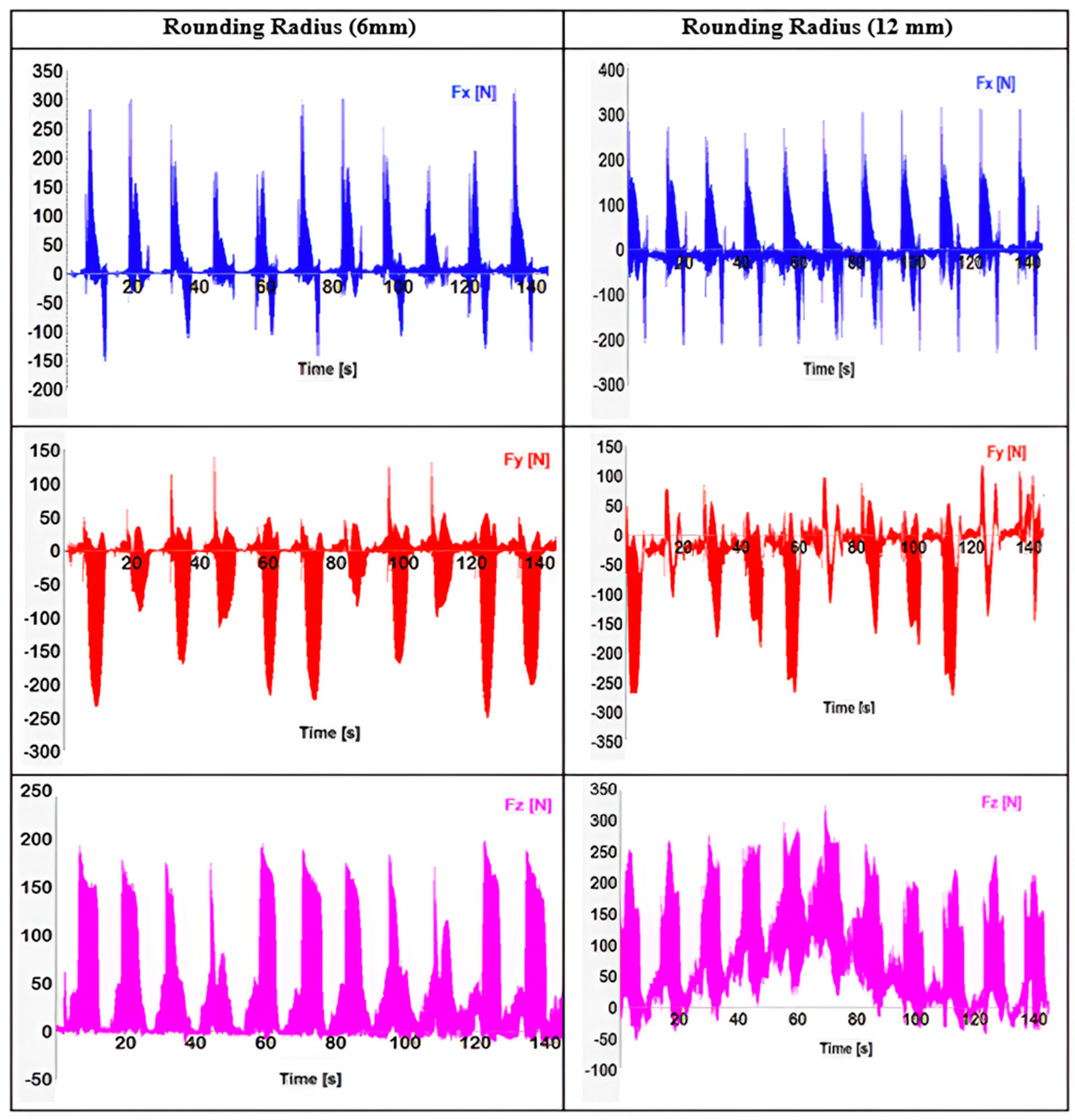
The increase in cutting speed from 50 to 90 m/min caused a decrease in resultant cutting force because of reduced tool–work piece friction as shown in Figure 10a. The increased radius of the trochoidal loop resulted in higher cutting forces because the tool created a larger cutting engagement loop which generated higher forces, as Figure 11 shows. Figure 10b reveals that the resultant force rises when the feed rate rises from 0.05 to 0.15 mm/tooth since the cutting tool faced larger tool path loop radii that created greater stress on the tooltip. The higher Ra became a consequence of these conditions. When the cutting tool tip entered the disengagement stage it experienced cooling which decreased tool wear rates [28].

3.4. Effect of Rounding Radius on Nose Wear

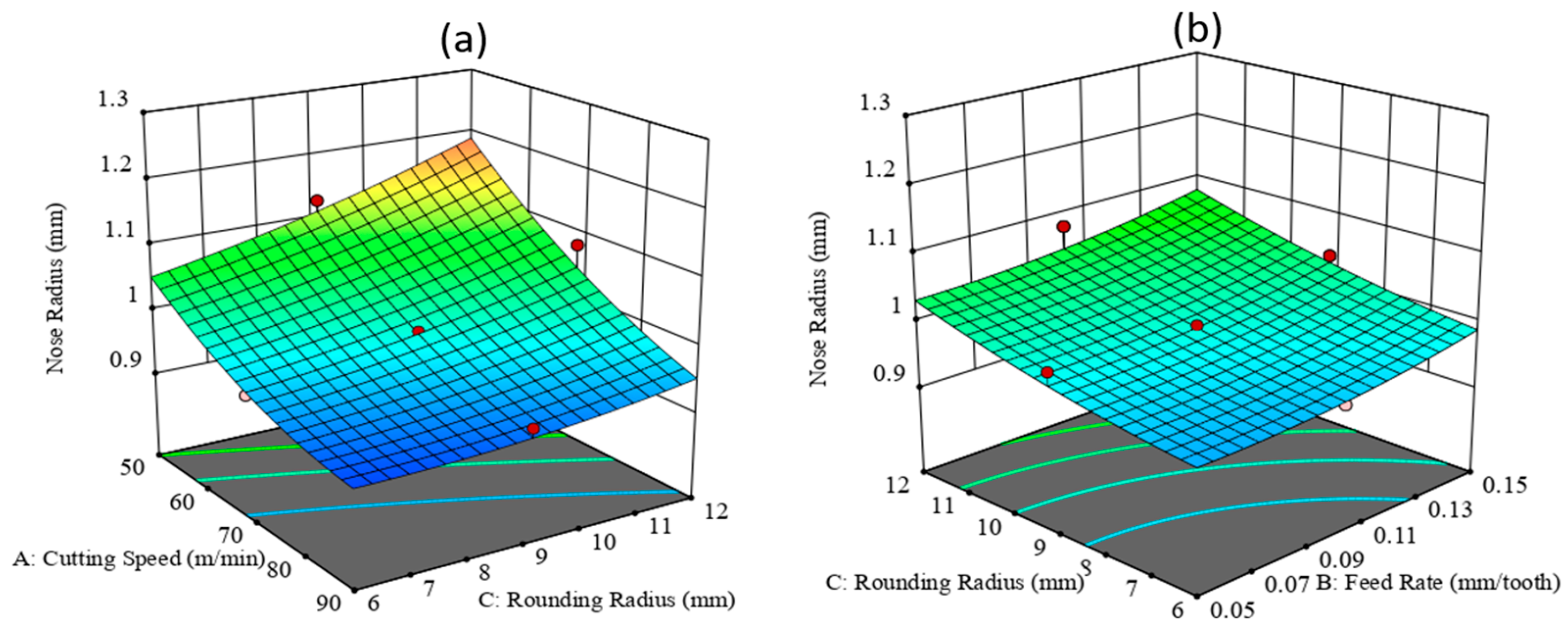
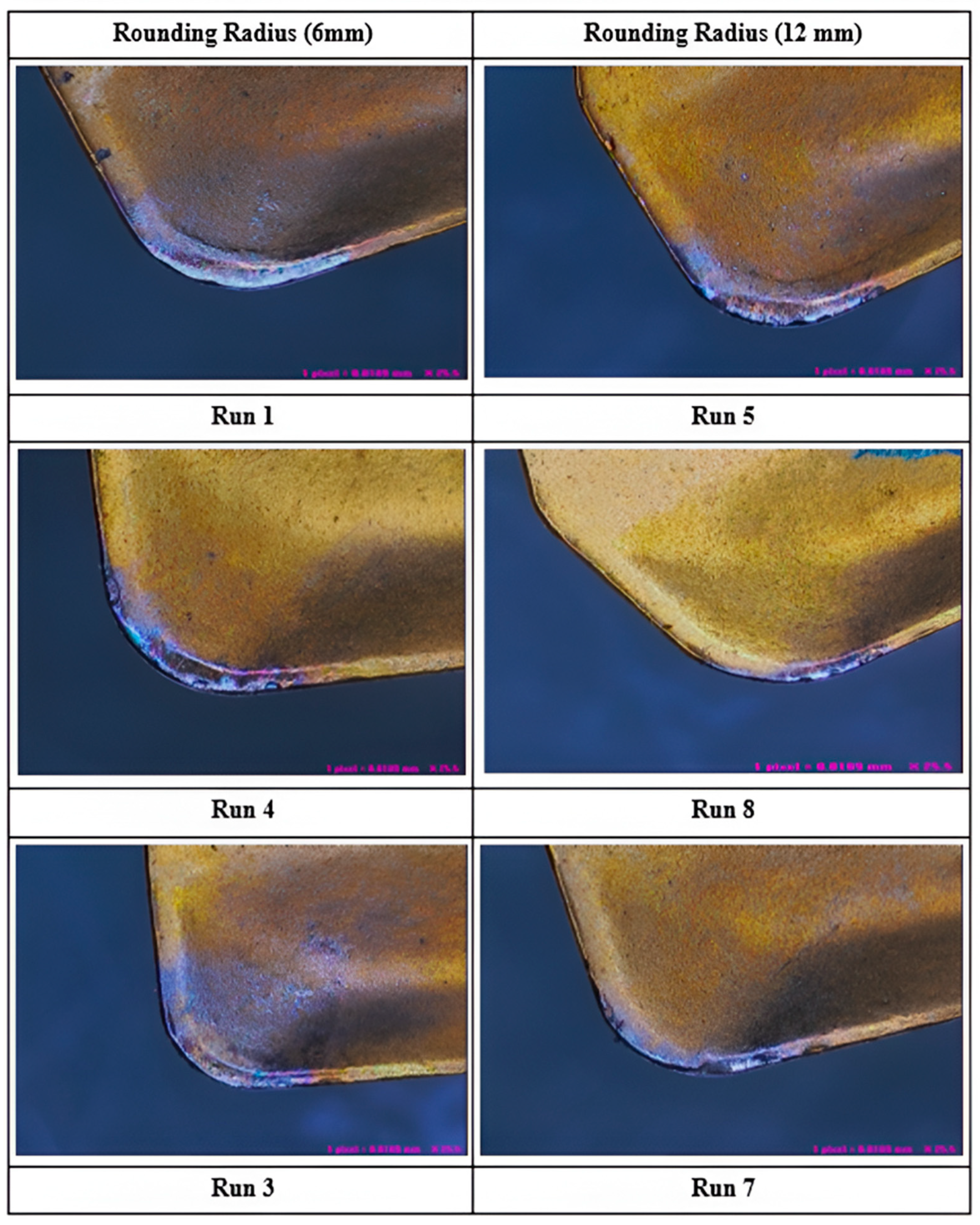
Nose wear of the tool developed at the mating interface of face and flank where both flank and crater wear combine to generate this effect. The tool corners feature their distinct area of wear which serves as a fundamental component for maintaining correct workpiece cutting. Figure 12a demonstrates that nose radius wear reduces when cutting speed advances from 50 m/min to 90 m/min due to friction yet the increase in trochoidal rounding radius from 6 mm to 12 mm leads to increased wear of the nose because of elevated tooltip engagement. The data in Figure 12b illustrate that nose wear grows proportionally with feed rate increases between 0.05 and 0.15 mm/tooth. Figure 13 demonstrates tool tip deformation taking place at the cutting edge because the coating layer has suffered to peel off. The tool edge micro-geometry caused irregularities on the tooltip surface which led to an increased deviation of the initial nose radius. The cutting process exposes the flank face to higher exposure due to friction between chips and workpieces which forms a built-up edge on the crater face [29].

3.5. Chip Morphology Studies

Figure 14 demonstrates the obtained lamella structure of trochoidal rounding radius (6 mm and 12 mm) with a cutting speed of 90 m/min and feed rate set at 0.15 mm/tooth. The basic feature of the back surface chip structure appears rough and jagged due to shearing action. The tool engagement angle reduces throughout the process when the trochoidal rounding radius has low distance travel which results in reduced cutting load. The formation of a uniform lamella structure takes place. At a 12 mm rounding radius, a non-uniform lamella structure was observed. The shearing forces within the cutting zone become very intense when exposed to this condition. The tooltip feels greater vibration while increasing the trochoidal rounding radius and this leads to a continual force increase that allows material shearing. The back surface of the chip undergoes high pressure and friction with the tool rake face due to this chip motion which produces non-uniform lamellar structures.

3.6. Genetic Algorithm Optimization

The GA functions as a technique for metaheuristic optimization to solve problems with and without constraints. The GA performs an artificial representation of both natural selection and genetic inheritance systems. The algorithm makes population-wide modifications through the selection process of randomly chosen individuals from the current generation. The procedure uses population members as parental entities to create offspring series until it reaches the optimal solution. The calculation of updating the population relies on random number generation. The next generation only receives superior characteristics that emerge from within the population. The prediction of optimized input parameters relies on the GA which proves itself as an efficient optimization tool in various manufacturing sectors [30]. A step-by-step procedure for GA optimization studies features in the following algorithm.

• A random population is initialized;
• Objective function estimation;
• Fitness function determination;
• The optimization process runs until termination criteria become met where GA operators, including reproduction, crossover rate, and mutation, are activated.

An implementation of GA optimization in version 2.5 of Neural Power Professional software was made. A function derived through ANN learning was fed into the GA module for processing. The researchers have chosen the GA parameters similar to prior works as presented in

Table 10. GA input parameters.

Subject	Values
Population size	100
Selection type:	Roulette method
Crossover type:	Single Point Crossover
Mutation rate	0.01
Cross overrate	0.5
Constrained range for cutting speed	50 and 90 m/min
Constrained range for feed rate	0.05 and 0.15 mm/tooth
Constrained range for rounding radius	6 to 12 mm
Objective function	Minimization

of reference [31].

The developed ANN model was used in conjunction with the Genetic Algorithm to search for effective parameterization within the boundaries created for the search space. The GA is normally dedicated for use of multi objective optimization problems, but when applied to this research, it conforms to the necessity to tackle the complex nonlinearities of the output and interdependent nature of the input variables. By acting as a surrogate model to the objective function, ANN facilitated extensive ranges of parameter space exploration. The standard configuration of the GA (100 population, 0.5 crossover rate, and 0.01 mutation rate) complies with the previous optimization approaches in manufacturing, and it was successful, as proved by minimal error margins of 6.49% between experimental and predicted values for surface roughness, 4.26% for cutting force, and 4.1% for nose radius wear on the validation tests despite the small dataset.

3.7. Confirmation Test

Table 11. Confirmation run results.

Experiment	Cutting Speed (m/min)	Feed Rate (mm/tooth)	Rounding Radius (mm)	Surface Roughness (µm)	Cutting Force (N)	Nose Wear (mm)
GA solution	85.01	0.0713	7.314	0.879	426.019	0.90
Feasible solution	85	0.07	7	-	-	-
Confirmation test results	85	0.07	7	0.94	445.14	0.93
Percentage error (%)				6.49	4.26	4.1

presents the results obtained from a feasible solution when running the confirmation test. It demonstrated that the experimental data of mean Ra (0.879 μm), cutting force (426.019 N), and nose radius wear (0.90 mm) had a very close match with the GA predicted values of mean Ra (0.94 μm), cutting force (445.14 N), and nose radius wear (0.93 mm) with minimal deviation during the given range of input parameters.

4. Conclusions

The present work developed an ANN model for end milling operation on surface roughness, resultant cutting force, and nose radius wear using a trochoidal toolpath strategy for AISI D3 steel. Experimental trials happened according to face-centered central composite design structures which follow response surface methodology principles. The following findings were observed:

• The combination of the LMBP learning algorithm with ten neurons in the hidden layer produced the lowest 0.40388 RMSE value from all considered ANN learning methods. Simulation results showed that the model inside its trained boundaries demonstrated effective performance as a prediction tool for output responses.
• The experimental results indicated that the feed rate along with trochoidal rounding radius and cutting speed established 42%, 26%, and 28% as the key parameters for the study.
• The tool edge micro-geometry caused irregularities on the tooltip surface which led to a 33.82% deviation of initial nose radius.
• Surface roughness deteriorated because of defective conditions that included cracks, feed marks, and side flow marks of the machined surface.
• Increasing of trochoidal rounding radius affects both chip formation and evacuation while machining takes place. The basic feature of the back surface chip structure appeared rough and jagged due to shearing action. The back surface of the chip undergoes high pressure and friction with the tool rake face due to this chip motion which produces non-uniform lamellar structures.
• The tool engagement angle was reduced throughout the process when the trochoidal rounding radius had low distance travel which resulted in reduced cutting load.
• The GA enabled the finding of optimal parameters consisting of 85 m/min for cutting speed and 0.07 mm/tooth for feed rate as well as 7 mm for trochoidal rounding radius which resulted in a minimal 6.49% error between experimental and predicted values for surface roughness, 4.26% for cutting force, and 4.1% for nose radius wear.
• The application of the adaptive trochoidal toolpath in combination with the Artificial Neural Network-Gentile algorithm enables several practical advantages for such industries as die and mold production, aerospace, automobile manufacture, etc. With this toolpath technology, machining of difficult materials and complex designs becomes a possibility, leading to faster machining processes, prolonged tool life, and enhanced surface quality when it comes to slotting, pocketing, and cavity milling. The implementation of this method will lead to more reliable, economical, and superior manufacturing results in vibrating environments with high demands of production output. Adoption of these optimum settings results in greater machined component quality.

References

1. Varghese, A.; Kulkarni, V.; Joshi, S.S. Modeling cutting edge degradation by chipping in micro-milling. Wear 2022, 488, 204141. [Google Scholar] [CrossRef]
2. Reddy, N.S.K.; Rao, P.V. Selection of an optimal parametric combination for achieving a better surface finish in dry milling using genetic algorithms. Int. J. Adv. Manuf. Technol. 2005, 28, 463–473. [Google Scholar] [CrossRef]
3. Santhakumar, J.; Iqbal, U.M. Parametric optimization of trochoidal step on surface roughness and dish angle in end milling of AISID3 steel using precise measurements. Materials 2019, 12, 1335. [Google Scholar] [CrossRef]
4. Ferreira, J.C.E.; Ochoa, D.M. A method for generating trochoidal tool paths for 2½D pocket milling process planning with multiple tools. Proc. Inst. Mech. Eng. B J. Eng. Manuf. 2013, 227, 1287–1298. [Google Scholar] [CrossRef]
5. Niaki, F.A.; Pleta, A.; Mears, L. Trochoidal milling: Investigation of a new approach on uncut chip thickness modeling and cutting force simulation in an alternative path planning strategy. Int. J. Adv. Manuf. Technol. 2018, 97, 641–656. [Google Scholar] [CrossRef]
6. Yan, R.; Li, H.; Peng, F.; Tang, X.; Xu, J.; Zeng, H. Stability prediction and step optimization of trochoidal milling. J. Manuf. Sci. Eng. 2017, 139, 091006. [Google Scholar] [CrossRef]
7. Wang, S.; Mei, W.; Liu, B.; Wang, C. Trochoidal machining for the high-speed milling of pockets. J. Mater. Process. Technol. 2016, 233, 29–43. [Google Scholar]
8. Uhlmann, E.; Fürstmann, P.; Rosenau, B. The potential of reducing the energy consumption for machining TiAl6V4 by using innovative metal cutting processes. In Proceedings of the 11th Global Conference on Sustainable Manufacturing, Berlin, Germany, 23–25 September 2013; pp. 593–598. [Google Scholar]
9. Pleta, A.; Ulutan, D.; Mears, L. Investigation of trochoidal milling in nickel-based superalloy Inconel 738 and comparison with end milling. In Proceedings of the ASME 2014 International Manufacturing Science and Engineering Conference, MSEC2014-4151, Detroit, MI, USA, 9–13 June 2014; p. V002T02A058. [Google Scholar]
10. Pleta, A.; Ulutan, D.; Mears, L. An investigation of alternative path planning strategies for machining of nickel-based superalloys. Procedia Manuf. 2015, 1, 556–566. [Google Scholar] [CrossRef]
11. Otkur, M.; Lazoglu, I. Trochoidal milling. Int. J. Mach. Tools Manuf. 2007, 47, 1324–1332. [Google Scholar] [CrossRef]
12. Edem, I.F.; Balogun, V.A.; Mativenga, P.T. An investigation on the impact of toolpath strategies and machine tool axes configurations on electrical energy demand in mechanical machining. Int. J. Adv. Manuf. Technol. 2017, 92, 2503–2509. [Google Scholar] [CrossRef]
13. Zeroudi, N.; Fontaine, M.; Necib, K. Prediction of cutting forces in 3-axes milling of sculptured surfaces directly from CAM tool path. J. Intell. Manuf. 2012, 23, 1573–1587. [Google Scholar] [CrossRef]
14. Topal, E.S. The role of stepover ratio in prediction of surface roughness in flat end milling. Int. J. Mech. Sci. 2009, 51, 782–789. [Google Scholar] [CrossRef]
15. Palanisamy, P.; Rajendran, I.; Shanmugasundaram, S. Prediction of tool wear using regression and ANN models in end-milling operation. Int. J. Adv. Manuf. Technol. 2008, 37, 29–41. [Google Scholar] [CrossRef]
16. Mia, M.; Khan, M.A.; Dhar, N.R. Study of surface roughness and cutting forces using ANN, RSM, and ANOVA in turning of Ti-6Al-4V under cryogenic jets applied at flank and rake faces of coated WC tool. Int. J. Adv. Manuf. Technol. 2017, 93, 975–991. [Google Scholar] [CrossRef]
17. Kannan, T.D.B.; Ramesh, T.; Sathiya, P. Application of artificial neural network modeling for optimization of Yb: YAG laser welding of Nitinol. Trans. Indian Inst. Met. 2017, 70, 1763–1771. [Google Scholar] [CrossRef]
18. Babu, K.K.; Panneerselvam, K.; Sathiya, P.; Haq, A.N.; Sundarrajan, S.; Mastanaiah, P.; Murthy, C.V.S. Parameter optimization of friction stir welding of cryo-rolled AA2219 alloy using artificial neural network modeling with genetic algorithm. Int. J. Adv. Manuf. Technol. 2018, 94, 3117–3129. [Google Scholar] [CrossRef]
19. Pimenov, D.; Bustillo, A.; Mikolajczyk, T. Artificial intelligence for automatic prediction of required surface roughness by monitoring wear on face mill teeth. J. Intell. Manuf. 2018, 29, 1045–1061. [Google Scholar] [CrossRef]
20. Quintana, G.; Garcia-Romeu, M.L.; Ciurana, J. Surface roughness monitoring application based on artificial neural networks for ball-end milling operations. J. Intell. Manuf. 2011, 22, 607–617. [Google Scholar] [CrossRef]
21. Zagórski, I.; Kulisz, M.; Kłonica, M.; Matuszak, J. Trochoidal milling and neural networks simulation of magnesium alloys. Materials 2019, 12, 2070. [Google Scholar] [CrossRef]
22. Munoz-Escalona, P.; Maropoulos, P.G. Artificial neural networks for surface roughness prediction when face milling Al 7075-T7351. J. Mater. Eng. Perform. 2010, 19, 185–193. [Google Scholar] [CrossRef]
23. Zain, A.M.; Haron, H.; Sharif, S. Integrated ANN–GA for estimating the minimum value for machining performance. Int. J. Prod. Res. 2012, 50, 191–213. [Google Scholar] [CrossRef]
24. Öktem, H. An integrated study of surface roughness for modeling and optimization of cutting parameters during the end milling operation. Int. J. Adv. Manuf. Technol. 2009, 43, 852–861. [Google Scholar] [CrossRef]
25. Zain, A.M.; Haron, H.; Sharif, S. Application of GA to optimize cutting conditions for minimizing surface roughness in end milling machine process. Expert Syst. Appl. 2010, 37, 4650–4659. [Google Scholar] [CrossRef]
26. Liu, Z.Y.; Guo, Y.B.; Sealy, M.P.; Liu, Z.Q. Energy consumption and process sustainability of hard milling with tool wear progression. J. Mater. Process. Technol. 2016, 229, 305–312. [Google Scholar] [CrossRef]
27. Abdu, H.; Mohamed, S.; Morad, A.A.E.M.; Elhameed, A.; Wazeer, A.E.; Moustafa, M.M. Modeling and optimization of process parameters for surface roughness and cutting forces on end milling using RSM and Taguchi method. J. Mod. Res. 2024, 6, 14–20. [Google Scholar] [CrossRef]
28. Zhou, K.; Zhang, C.; Du, S. Cutting force prediction for trochoid milling of 300M ultra-high strength steel. Processes 2022, 10, 2617. [Google Scholar] [CrossRef]
29. Shiva, P.N.; Padmakumar, M.; Sarada, B.N. Experimental investigation to assess the effects of trumpet hone on tool life and surface quality in milling of AISI4140 steel. FME Trans. 2019, 47, 437–441. [Google Scholar] [CrossRef]
30. Anand, B.K.; Barik, B.K.; Tamilmannan; Sathiya, P. Artificial neural network modeling studies to predict the friction welding process parameters of Incoloy 800H joints. Eng. Sci. Technol. Int. J. 2015, 18, 394–407. [Google Scholar] [CrossRef]
31. Ktema, O.H.; Erzurumlu, T.; Kurtaran, H. Application of response surface methodology in the optimization of cutting conditions for surface roughness. J. Mater. Process. Technol. 2005, 170, 11–16. [Google Scholar]
Figure 1. (ac) Trochoidal rounding radius simulation.
Jmmp 09 00171 g001
Figure 2. Experimental setup and calibration equipment.
Jmmp 09 00171 g002
Figure 3. Zoller tool pre-setter for determination of the nose radius variation.
Jmmp 09 00171 g003
Figure 4. Step-by-step process of ANN—GA methodology.
Jmmp 09 00171 g004
Figure 5. (ac) Predicted versus experimental data scatter plots for output responses.
Jmmp 09 00171 g005
Figure 6. ANN structure.
Jmmp 09 00171 g006
Figure 7. Significance of input factors.
Jmmp 09 00171 g007
Figure 8. (a,b) Ra—3D factorial interaction surface plots.
Jmmp 09 00171 g008
Figure 9. Effect of rounding radius (6 mm and 12 mm) on Ra at Cutting speed-90 m/min, Feed rate-0.15 mm/tooth.
Jmmp 09 00171 g009
Figure 10. (a,b) Fc—3D factorial interaction surface plots.
Jmmp 09 00171 g010
Figure 11. Effect of rounding radius (6 mm and 12 mm) on cutting force (Fx, Fy, and Fz) at Cutting speed-90 m/min, Feed rate-0.15 mm/tooth.
Jmmp 09 00171 g011
Figure 12. (a,b) Nose radius wear—3D factorial interaction surface plots.
Jmmp 09 00171 g012
Figure 13. Effect of rounding radius on nose wear by VMS.
Jmmp 09 00171 g013
Figure 14. Chip and lamella structure of rounding radius (6 mm and 12 mm) at Cutting speed-90 m/min, Feed rate-0.15 mm/tooth.
Jmmp 09 00171 g014