
New Input Factors for Machine Learning Approaches to Predict the Weld Quality of Ultrasonically Welded Thermoplastic Composite Materials

 , ,
, ,
Abstract
1. Introduction
1.1. Quality Assurance in Ultrasonic Welding
1.2. Parameter Research
1.2.1. Thermography
1.2.2. Acoustic Signals
2. Materials and Methods
2.1. Experimental Setup
2.2. Data Processing and Analysis Steps
2.2.1. Acoustic Signals
2.2.2. Thermography
2.3. Machine Learning
- Duration of welding (number of measured data points of one parameter);
- Mean temperature of a thermal image;
- Peak amplitude of the FFT of the 2 kHz bin of data;
- Peak amplitude of the FFT of the 20 kHz bin of data.
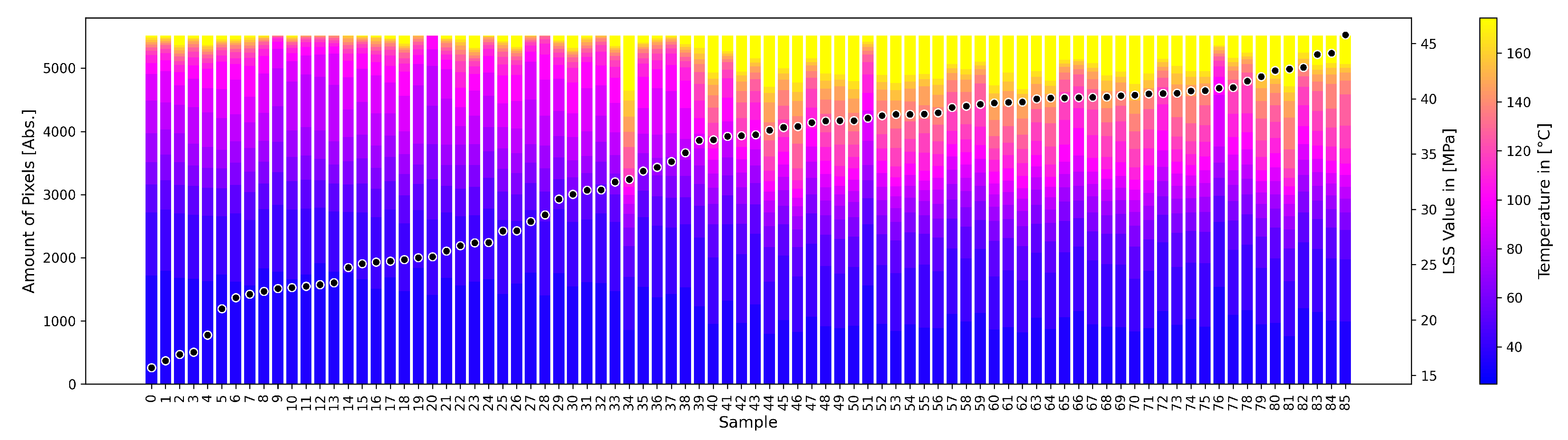
3. Results
4. Discussion
5. Conclusions
Author Contributions
Funding

Data Availability Statement
Conflicts of Interest
Abbreviations
| TCs | thermoplastic composites |
| UW | ultrasonic welding |
| CUW | continuous ultrasonic welding |
| SPW | spot welding |
| ML | machine learning |
| AI | artificial intelligence |
| FEM | finite element model |
| LSTM | long short-term memory |
| RF | random forest |
| ED | energy director |
| NDT | non-destructive testing |
| GFRP | glass-fiber-reinforced polymers |
| CFRP | carbon-fiber-reinforced polymers |
| AE | acoustic emission |
| SE | sound emission |
| DOE | design of experiment |
| LSS | lab-shear-strength |
| FFT | fast Fourier transformation |
| ROI | region of interest |
| KNN | k-nearest-neighbor |
| RF | random forest |
| SVM | support vector machine |
Appendix A. Spearman Correlation Coefficients of the Sound Data

| Frequency Bin (kHz) | Correlation Coefficient | p-Value | Number of Samples |
|---|---|---|---|
| 0.698330539 | 87 | ||
| 0.259039878 | 0.015404615 | 87 | |
| −0.332253046 | 0.011567735 | 57 | |
| 0.4 | 0.22286835 | 11 | |
| −0.067653277 | 0.666429017 | 43 | |
| −0.047619048 | 0.910849169 | 8 | |
| −0.225225225 | 0.180159238 | 37 | |
| 0.182237469 | 0.187200228 | 54 | |
| 0.238961039 | 0.296849183 | 21 | |
| 0.601170081 | 87 | ||
| - | - | 0 | |
| - | - | 0 |
| Frequency Bin (kHz) | Correlation Coefficient | p-Value | Number of Samples |
|---|---|---|---|
| 0.225452716 | 0.058705078 | 71 | |
| 0.376102418 | 0.000882821 | 75 | |
| 0.288141026 | 0.020949089 | 64 | |
| −0.03 | 0.886801818 | 25 | |
| −0.165722344 | 0.198001899 | 62 | |
| −0.018181818 | 0.957685241 | 11 | |
| 0.197192513 | 0.271353653 | 33 | |
| 0.252613936 | 0.039169609 | 67 | |
| −0.145894428 | 0.425599249 | 32 | |
| 0.699861486 | 87 | ||
| - | - | 0 | |
| −0.028571429 | 0.957154519 | 6 |
References
- Arul, S.; Vijayaraghavan, L.; Malhotra, S.K. Online monitoring of acoustic emission for quality control in drilling of polymeric composites. J. Mater. Process. Technol. 2007, 185, 184–190. [Google Scholar] [CrossRef]
- Slayton, R.; Spinardi, G. Radical innovation in scaling up: Boeing’s Dreamliner and the challenge of socio-technical transitions. Technovation 2016, 47, 47–58. [Google Scholar] [CrossRef]
- Chawla, K.K. Carbon Fiber Composites; Composite Materials: Science and Engineering; Springer Science+Business Media: New York, USA, 1998; pp. 252–277. [Google Scholar]
- Marani, R.; Palumbo, D.; Galietti, U.; Stella, E.; D’Orazio, T. Automatic Detection of Subsurface Defects in Composite Materials using Thermography and Unsupervised Machine Learning. In Proceedings of the 2016 IEEE 8th International Conference on Intelligent Systems (IS), Sofia, Bulgaria, 4–6 September 2016; pp. 516–521. [Google Scholar] [CrossRef]
- Yang, B.; Wang, C. Thermal Nondestructive Testing Technology of Aircraft Composite Material. In Proceedings of the 2009 9th International Conference on Electronic Measurement & Instruments, Beijing, China, 16–19 August 2009; pp. 2-557–2-562. [Google Scholar] [CrossRef]
- Yousefpour, A.; Hojjati, M.; Immarigeon, J.P. Fusion Bonding/Welding of Thermoplastic Composites. J. Thermoplast. Compos. Mater. 2004, 17, 303–341. [Google Scholar] [CrossRef]
- Zhang, Z.; Wang, X.; Luo, Y.; Zhang, Z.; Wang, L. Study on Heating Process of Ultrasonic Welding for Thermoplastics. J. Thermoplast. Compos. Mater. 2010, 23, 647–664. [Google Scholar] [CrossRef]
- Bhudolia, S.K.; Gohel, G.; Leong, K.F.; Islam, A. Advances in Ultrasonic Welding of Thermoplastic Composites: A Review. Materials 2020, 13, 1284. [Google Scholar] [CrossRef] [PubMed]
- Toray. Toray Advanced Composites, Cetex® TC1225 LMPAEK. 2022. Data Sheet. pp. 1–7. Available online: https://www.toraytac.com/product-explorer/products/gXuK/Toray-Cetex-TC1225. (accessed on 17 August 2023).
- Baur, S.; Hader, M.; Gautier, D. On a Wing and a Prayer? Challenges and Opportunities in the Aerostructure Supplier Industry; Roland Berger GmbH: Munich, Germany, 2019. [Google Scholar]
- Villegas, I.F.; Bersee, H.E.N. Ultrasonic Welding of Advanced Thermoplastic Composites: An Investigation on Energy-Directing Surfaces. Adv. Polym. Technol. 2010, 29, 112–121. [Google Scholar] [CrossRef]
- Villegas, I.F. Ultrasonic Welding of Thermoplastic Composites. Front. Mater. 2019, 6, 291. [Google Scholar] [CrossRef]
- Nonhof, C.J.; Luiten, G.A. Estimates for Process Conditions During the Ultrasonic Welding of Thermoplastics. Polym. Eng. Sci. 1996, 36, 1177–1183. [Google Scholar] [CrossRef]
- Li, Y.; Liu, Z.; Shen, J.; Lee, T.H.; Banu, M.; Hu, S.J. Weld Quality Prediction in Ultrasonic Welding of Carbon Fiber Composite Based on an Ultrasonic Wave Transmission Model. J. Manuf. Sci. Eng. 2019, 141, 081010-1–081010-15. [Google Scholar] [CrossRef]
- Liu, S.J.; Chang, I.T.; Hung, S.W. Factors Affecting the Joint Strength of Ultrasonically Welded Polypropylene Composites. Polym. Compos. 2001, 22, 132–141. [Google Scholar] [CrossRef]
- Villegas, I.F. In situ monitoring of ultrasonic welding of thermoplastic composites through power and displacement data. J. Thermoplast. Compos. Mater. 2015, 28, 66–85. [Google Scholar] [CrossRef]
- Wang, K.; Shriver, D.; Li, Y.; Banu, M.; Hu, S.J.; Xiao, G.; Arinez, J.; Fan, H.T. Characterization of weld attributes in ultrasonic welding of short carbon fiber reinforced thermoplastic composites. J. Manuf. Process. 2017, 29, 124–132. [Google Scholar] [CrossRef]
- Jongbloed, B.; Teuwen, J.; Palardy, G.; Villegas, I.F.; Benedictus, R. Improving Weld Uniformity in Continuous Ultrasonic Welding of Thermoplasic Composites. In Proceedings of the ECCM18—18th European Conference on Composite Materials, Athens, Greece, 24–28 June 2018; pp. 1–8. [Google Scholar]
- Jongbloed, B.C.P. Continuous Ultrasonic Welding of Thermoplastic Composites: An Experimental Study Towards Understanding Factors Influencing Weld Quality. Ph.D. Thesis, Delft University of Technology, Delft, The Netherlands, 2022. [Google Scholar] [CrossRef]
- Lakshmanan, V.; Robinson, S.; Munn, M. Machine Learning Design Patterns: Solutions to Common Challenges in Data Preparation, Model Building, and MLOps; O’Reilly Media Inc.: Sebastopol, CA, USA, 2020. [Google Scholar]
- Li, Y.; Lee, T.H.; Wang, C.; Wang, K.; Tan, C.; Banu, M.; Hu, S.J. An artificial neural network model for predicting joint performance in ultrasonic welding of composites. In Proceedings of the 7th CIRP Conference on Assembly Technologies and Systems, Tianjin, China, 10–12 May 2018; Elsevier B.V.: Amsterdam, The Netherlands, 2018; Volume 76, pp. 85–88. [Google Scholar] [CrossRef]
- Wang, B.; Li, Y.; Luo, Y.; Li, X.; Freiheit, T. Early event detection in a deep-learning driven quality prediction model for ultrasonic welding. J. Manuf. Syst. 2021, 60, 325–336. [Google Scholar] [CrossRef]
- Li, Y.; Yu, B.; Wang, B.; Lee, T.H.; Banu, M. Online quality inspection of ultrasonic composite welding by combining artificial intelligence technologies with welding process signatures. Mater. Des. 2020, 194, 108912. [Google Scholar] [CrossRef]
- Larsen, L.; Görick, D.; Engelschall, M.; Fischer, F.; Kupke, M. Process data driven advancement of robot-based continuous ultrasonic welding for the dust-free assembly of future fuselage structures. In Proceedings of the International Conference and Exhibition on Thermoplastic Composites (ITHEC 2020), Bremen, Germany, 13–15 October 2020. [Google Scholar]
- Görick, D.; Larsen, L.; Engelschall, M.; Schuster, A. Quality Prediction of Continuous Ultrasonic Welded Seams of High-Performance Thermoplastic Composites by means of Artificial Intelligence. In Proceedings of the 30th International Conference on Flexible Automation and Intelligent Manufacturing (FAIM2021), Athens, Greece, 15–18 June 2021; Volume 55, pp. 116–123. [Google Scholar] [CrossRef]
- Görick, D. An Artificial Intelligence Approach for the Joint Strength Prediction of High-Performance Thermoplastic Composites. Master’s Thesis, Westfälische Hochschule, Bocholt, Germany, Performed at: German Aerospace Center (DLR), Center for Lightweight Production Technology, Augsburg, Germany. 2020. [Google Scholar]
- Ng, E.Y.K.; Fok, S.C.; Peh, Y.C.; Ng, F.C.; Sim, L.S.J. Computerized detection of breast cancer with artificial intelligence and thermograms. J. Med. Eng. Technol. 2002, 26, 152–157. [Google Scholar] [CrossRef]
- Bauer, J.; Hoq, M.N.; Mulcahy, J.; Tofail, S.A.M.; Gulshan, F.; Silien, C.; Podbielska, H.; Akbar, M.M. Implementation of artificial intelligence and non-contact infrared thermography for prediction and personalized automatic identification of different stages of cellulite. EPMA J. 2020, 11, 17–29. [Google Scholar] [CrossRef]
- Jadin, M.S.; Taib, S. Recent progress in diagnosing the reliability of electrical equipment by using infrared thermography. Infrared Phys. Technol. 2012, 55, 236–245. [Google Scholar] [CrossRef]
- Favro, L.D.; Thomas, R.L.; Han, X.; Ouyang, Z.; Newaz, G.; Gentile, D. Sonic infrared imaging of fatigue cracks. Int. J. Fatigue 2001, 23, 471–476. [Google Scholar] [CrossRef]
- Ranjit, S.; Kang, K.; Kim, W. Investigation of Lock-in Infrared Thermography for Evaluation of Subsurface Defects Size and Depth. Int. J. Precis. Eng. Manuf. 2015, 16, 2255–2264. [Google Scholar] [CrossRef]
- Montanini, R.; Freni, F. Non-destructive evaluation of thick glass fiber-reinforced composites by means of optically excited lock-in thermography. Compos. Part A Appl. Sci. Manuf. 2012, 43, 2075–2082. [Google Scholar] [CrossRef]
- Yang, B.; Huang, Y.; Cheng, L. Defect detection and evaluation of ultrasonic infrared thermography for aerospace CFRP composites. Infrared Phys. Technol. 2013, 60, 166–173. [Google Scholar] [CrossRef]
- Mian, A.; Han, X.; Islam, S.; Newaz, G. Fatigue damage detection in graphite/epoxy composites using sonic infrared imaging technique. Compos. Sci. Technol. 2004, 64, 657–666. [Google Scholar] [CrossRef]
- Palumbo, D.; Tamborrino, R.; Galietti, U.; Aversa, P.; Tatì, A.; Luprano, V.A.M. Ultrasonic analysis and lock-in thermography for debonding evaluation of composite adhesive joints. NDT E Int. 2016, 78, 1–9. [Google Scholar] [CrossRef]
- Junyan, L.; Liqiang, L.; Yang, W. Experimental study on active infrared thermography as a NDI tool for carbon–carbon composites. Compos. Part B Eng. 2013, 45, 138–147. [Google Scholar] [CrossRef]
- Rantala, J.; Wu, D.; Busse, G. Amplitude-Modulated Lock-In Vibrothermography for NDE of Polymers and Composites. Res. Nondestruct. Eval. 1996, 7, 215–228. [Google Scholar] [CrossRef]
- Gleiter, A.; Riegert, G.; Zweschper, T.; Busse, G. Ultrasound Lockin-Thermography for Advanced Depth Resolved Defect Selective Imaging. Insight-Non Test. Cond. Monit. 2006, 49, 272. [Google Scholar]
- Rizzo, P. Sensing solutions for assessing and monitoring underwater systems. In Sensor Technologies for Civil Infrastructures; Elsevier Ltd.: Pittsburgh, PA, USA, 2014; pp. 525–549. [Google Scholar]
- Goszczyńska, B.; Świt, G.; Trąmpczyński, W.; Krampikowska, A.; Tworzewska, J.; Tworzewski, P. Experimental validation of concrete crack identification and location with acoustic emission method. Arch. Civ. Mech. Eng. 2012, 12, 23–28. [Google Scholar] [CrossRef]
- Sause, M.G.R.; Scharringhausen, J.; Horn, S. Identification of Failure Mechanisms in Thermoplastic Composites by Acoustic Emission Measurements. In Proceedings of the 19th International Conference on Composite Materials, Montreal, QC, Canada, 28 July–2 August 2013. [Google Scholar]
- Srikanth, V.; Subbarao, E.C.; Agrawal, D.K.; Huang, C.Y.; Roy, R.; Rao, G.V. Thermal Expansion Anisotropy and Acoustic Emission of NaZr2P3O12 Family Ceramics. J. Am. Ceram. Soc. 1991, 74, 365–368. [Google Scholar] [CrossRef]
- Choi, D.G.; Choi, S.K. Dynamic behaviour of domains during poling by acoustic emission measurements in La-modified PbTiO3 ferroelectric ceramics. J. Mater. Sci. 1997, 32, 421–425. [Google Scholar] [CrossRef]
- Dunegan, H.; Harris, D. Acoustic emission-a new non destructive testing tool. Ultrasonics 1969, 7, 160–166. [Google Scholar] [CrossRef]
- Scruby, C.B. An introduction to acoustic emission. J. Phys. E Sci. Instrum. 1987, 20, 946–953. [Google Scholar] [CrossRef]
- Zhang, L.; Basantes-Defaz, A.D.C.; Abbasi, Z.; Yuhas, D.; Ozevin, D.; Indacochea, E. Real-time Nondestructive Monitoring of the Gas Tungsten Arc Welding (GTAW) Process by Combined Airborne Acoustic Emission and Non-Contact Ultrasonics. In Proceedings of the SPIE Smart Structures and Materials + Nondestructive Evaluation and Health Monitoring, Denver, CO, USA, 4–8 March 2018; Volume 10599. [Google Scholar] [CrossRef]
- Wasmer, K.; Le-Quang, T.; Meylan, B.; Shevchik, S.A. In Situ Quality Monitoring in AM Using Acoustic Emission: A Reinforcement Learning Approach. J. Mater. Eng. Perform. 2019, 28, 666–672. [Google Scholar] [CrossRef]
- Ali, Y.H.; Rahman, A.R.; Hamzah, R.I.R. Acoustic Emission Signal Analysis and Artificial Intelligence Techniques in Machine Condition Monitoring and Fault Diagnosis: A Review. J. Teknol. 2014, 69, 121–126. [Google Scholar] [CrossRef][Green Version]
- Choi, N.S.; Takahashi, K. Characterization of the damage process in short-fibre/thermoplastic composites by acoustic emission. J. Mater. Sci. 1998, 33, 2357–2363. [Google Scholar] [CrossRef]
- Garrett, J.C.; Mei, H.; Giurgiutiu, V. An Artificial Intelligence Approach to Fatigue Crack Length Estimation from Acoustic Emission Waves in Thin Metallic Plates. Appl. Sci. 2022, 12, 1372. [Google Scholar] [CrossRef]
- Wasmer, K.; Saeidi, F.; Meylan, B.; Vakili-Farahani, F.; Shevchik, S.A. When AE (Acoustic Emission) meets AI (Artificial Intelligence). In Proceedings of the 33nd European Conference on Acoustic Emission Testing, Senlis, France, 12–14 September 2018; pp. 1–8. [Google Scholar]
- Asif, K.; Zhang, L.; Derrible, S.; Indacochea, J.E.; Ozevin, D.; Ziebart, B. Machine learning model to predict welding quality using air-coupled acoustic emission and weld inputs. J. Intell. Manuf. 2022, 33, 881–895. [Google Scholar] [CrossRef]
- Li, L. A comparative study of ultrasound emission characteristics in laser processing. Appl. Surf. Sci. 2002, 186, 604–610. [Google Scholar] [CrossRef]
- Teledyne Flir. What Is the Relation between TemperatureLinearResolution and SensorGainMode (Temperature Range) for the FLIR Ax5 Series? Available online: https://www.flir.com/support-center/instruments2/what-is-the-relation-between-temperaturelinearresolution-and-sensorgainmode-temperature-range-for-the-flir-ax5-series/ (accessed on 28 July 2023).
- Fahrmeir, L.; Heumann, C.; Künstler, R.; Pigeot, I.; Tutz, G. Statistik: Der Weg zur Datenanalyse, 8th ed.; Springer: Berlin/Heidelberg, Germany, 2016. [Google Scholar] [CrossRef]
- scipy.stats.spearmanr. Available online: https://docs.scipy.org/doc/scipy/reference/generated/scipy.stats.spearmanr.html (accessed on 17 January 2023).
- FLIR Systems. User’s Manual FLIR Ax5 Series. 2016. Available online: https://www.globaltestsupply.com/pdfs/cache/www.globaltestsupply.com/75010-0101/manual/75010-0101-manual.pdf (accessed on 17 January 2023).


| Channel | Frequ. Bin (kHz) | Corr Coef | p-Value | Num. of Samples |
|---|---|---|---|---|
| 0.698 | 87 | |||
| 0.259 | 0.015 | 87 | ||
| −0.332 | 0.012 | 57 | ||
| 0.182 | 0.187 | 54 | ||
| 0.601 | 87 | |||
| 0.225 | 0.059 | 71 | ||
| 0.376 | 0.001 | 75 | ||
| 0.288 | 0.021 | 64 | ||
| −0.166 | 0.198 | 62 | ||
| 0.253 | 0.039 | 67 | ||
| 0.7 | 87 |
Disclaimer/Publisher’s Note: The statements, opinions and data contained in all publications are solely those of the individual author(s) and contributor(s) and not of MDPI and/or the editor(s). MDPI and/or the editor(s) disclaim responsibility for any injury to people or property resulting from any ideas, methods, instructions or products referred to in the content. |
© 2023 by the authors. Licensee MDPI, Basel, Switzerland. This article is an open access article distributed under the terms and conditions of the Creative Commons Attribution (CC BY) license (https://creativecommons.org/licenses/by/4.0/).
Share and Cite
Görick, D.; Schuster, A.; Larsen, L.; Welsch, J.; Karrasch, T.; Kupke, M. New Input Factors for Machine Learning Approaches to Predict the Weld Quality of Ultrasonically Welded Thermoplastic Composite Materials. J. Manuf. Mater. Process. 2023, 7, 154. https://doi.org/10.3390/jmmp7050154
Görick D, Schuster A, Larsen L, Welsch J, Karrasch T, Kupke M. New Input Factors for Machine Learning Approaches to Predict the Weld Quality of Ultrasonically Welded Thermoplastic Composite Materials. Journal of Manufacturing and Materials Processing. 2023; 7(5):154. https://doi.org/10.3390/jmmp7050154
Chicago/Turabian StyleGörick, Dominik, Alfons Schuster, Lars Larsen, Jonas Welsch, Tobias Karrasch, and Michael Kupke. 2023. "New Input Factors for Machine Learning Approaches to Predict the Weld Quality of Ultrasonically Welded Thermoplastic Composite Materials" Journal of Manufacturing and Materials Processing 7, no. 5: 154. https://doi.org/10.3390/jmmp7050154
APA StyleGörick, D., Schuster, A., Larsen, L., Welsch, J., Karrasch, T., & Kupke, M. (2023). New Input Factors for Machine Learning Approaches to Predict the Weld Quality of Ultrasonically Welded Thermoplastic Composite Materials. Journal of Manufacturing and Materials Processing, 7(5), 154. https://doi.org/10.3390/jmmp7050154