1. Introduction
Fused deposition modeling (FDM) is one of the most popular types of additive manufacturing (AM), wherein a nozzle mechanically extrudes molten thermoplastic or metal materials layer by layer to generate three-dimensional surfaces or objects. Owing to its simplicity and flexibility, FDM printing has been widely used in various fields such as mechanical engineering, aerospace, and even biological engineering [
1]. Traditionally, three-axis AM systems with three degree-of-freedom (DOF) are used for printing simple-featured objects, in which the part is accumulated in planar layers along a fixed nozzle orientation. This feature leads to an easy-handle fabrication process, while it also brings problems such as the stair-case effect, the need for support for overhang features, weak mechanical strength, and restriction of printing motions [
2]. The advent multi-axis AM provides a considerably significant solution to resolve these problems. In general, for the multi-axis AM with additional DOFs, the nozzle axis does not have to align with the
z-axis, and neither do adjacent printing paths have to lie in a same plane [
3]. By carefully adjusting the nozzle orientation with respect to the surface normal, the defects such as the stair-case effect, local gouging problem, and the need for support that existed in three-axis printing can be eliminated, at least in theory.
Research in FDM AM is primarily focused on the following three principal issues: (1) the deposited materials, (2) the mechanism of hardware, and (3) the tool path planning and process control. Among the three, tool path planning/process control can be regarded as the most important module in terms of popularizing the AM technology. In the multi-axis case, efficient printing process planning, especially path planning, has always been a bottleneck due to the involvement of the additional rotary axes and the greatly increased complexity of the design models. Accordingly, specifically for 6-DOF robotic FDM printing, this paper presents an algorithm to automatically generate printing paths for efficiently printing an arbitrary freeform layer surface.
Due to the newness of multi-axis printing, there are few published research works about the multi-axis curved layer printing path generation. Dai et al. [
4] proposed to use Fermat spiral curves as a printing path to cover a given curved surface; however, as evidently illustrated in [
5], there exist uneven fills between filaments which may be detrimental to the attachment between the filaments and decreasing the strength of the printed object. Hence, such a pattern is much more suitable for a surface that is geometrically within holes and has a low requirement on filling quality. Chen et al. [
6] adopted the iso-parametric method to plan a tool path in the parametric domain of the surface, which though does not consider the printing efficiency issue and may generate a skewed and poor-quality tool path if the parametrization or transformation are inappropriate. Recently, Li et al. [
7] proposed using iso-geodesic distance contours as filling paths where a constant step-over between adjacent paths is ensured. However, this method by nature is specially designed to be boundary-conformal and, thus, does not consider the printing efficiency issue. Some prior studies [
8,
9,
10,
11] indeed have already attempted to improve the printing performance from different aspects, such as geometric accuracy, mechanical characteristics, and printing efficiency; nevertheless, they mainly considered these problems from the perspective of the workpiece, but not the printing system used for execution (e.g., the robotic manipulator) which though is directly related to the printing efficiency.
Targeting the aforementioned caveats, in this paper, an iso-planar type printing path planning method is proposed to improve the printing efficiency in consideration of the kinematical capacities of the printing system, as inspired by the well-known similar ideas in the realm of computer numerical control (CNC) machining. For instance, the machining potential field (MPF) method was first introduced by Chiou and Lee [
12] for tool path generation. By constructing the potential field on the sculptured surface, it is dedicated to improving the machining efficiency by finding the optimal feed direction maximizing the feasible machining strip width. Extended from this idea, several studies [
13,
14,
15] offered new optimal feed direction identification strategies, such as the work of Hu and Tang [
15], which defined a vector field on the workpiece surface that encapsulates the relationship between the material removal rate and the feed direction, considering both the local geometry and the machine axes’ physical limits. However, these works in tool path generation are only suitable for machining, which is a material removal process, while printing is a material buildup process which is exactly opposite to machining in terms of how the final shape of a workpiece is formed. Therefore, in the proposed method, we focused on seeking an efficiency-optimized feed direction to generate a multi-axis printing path. Specifically, we first propose a printing efficiency indicator called the material deposition rate which considers both the local geometry of the printing layer surface and the kinematical capacities of the robotic FDM printer. By maximizing this indicator globally, the best drive plane direction is found next, based on which the classic iso-planar method is then employed to generate the printing paths for the layer surface.
The paper proceeds following the steps outlined as shown in
Figure 1. First, in
Section 2, we introduce a sampling-based indicator that encapsulates both the effective printing width and the kinematics-constrained feed rate. Then, in
Section 3, we present the details of our iso-planar printing path generation method based on the proposed indicator. The results of the experiments and discussion are reported in
Section 4, followed by the conclusion in
Section 5.
2. Material Deposition Rate
Similar to five-axis milling, when planning a multi-axis printing path, both the nozzle location (NL) curves and the associated nozzle orientation need to be properly determined. In this section, we described in detail how to determine the effective printing width and the kinematic-constrained feed rate, which subsequently leads to the proposed indicator to evaluate the printing efficiency, i.e., the material deposition rate as a function of the feed direction .
2.1. Effective Printing Width
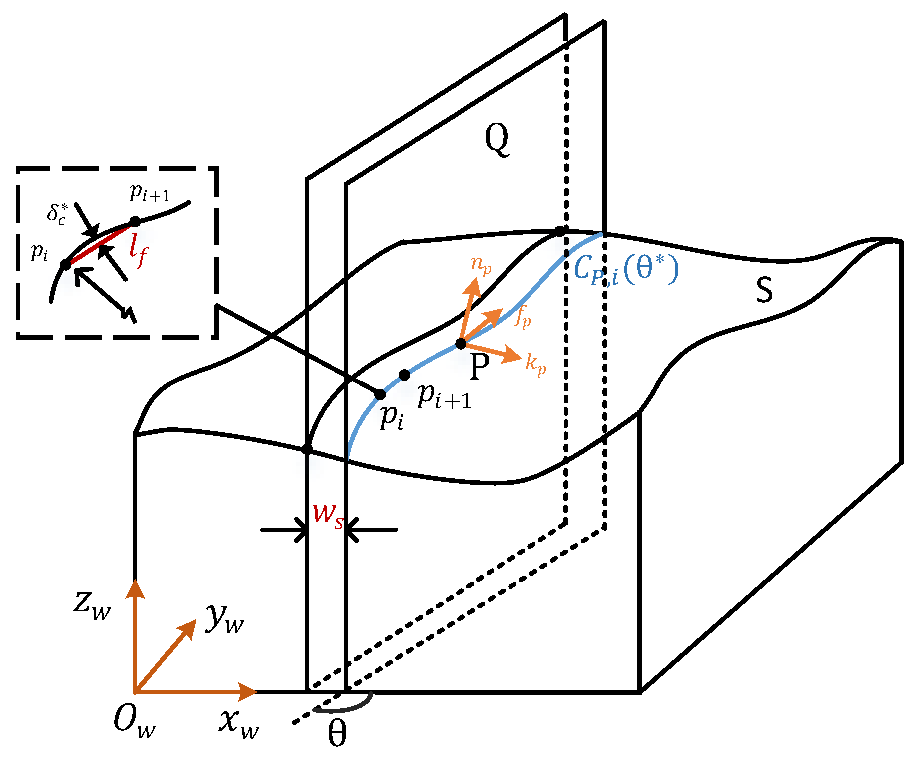
As shown in
Figure 2, numerically, a single NL curve (e.g.,
) identifies the nozzle movement during a printing process, which typically is represented as a series of sample points {
} with respect to the workpiece coordinate system (WCS) wherein the workpiece (i.e., the layer surface
S) is defined. At the same time, a standard local frame
-
-
is naturally defined at each point
on
where
is an angular parameter that determines the drive plane of this NL curve (see
Section 2.3), while
and
are the feed direction and normal direction of the surface at
, respectively, and
is the cross product of the former two.
In the realm of FDM printing, some previous research [
16,
17,
18,
19] studied various characteristics of the FDM process, and many mathematical models were proposed for the modeling of the geometry of the deposed material. Of all the proposed methods for modeling the cross-sectional shape of the deposited filaments, the ellipse model, which was originally proposed by Ahn et al. [
17] and subsequently extended by Angelo1 et al. [
19] with experimental validation, is commonly adopted. Therefore, the ellipse model is also adopted by us in this paper, which represents the cross-section of adjacent NL curves by two intersected ellipses. It should be mentioned that, for a genuine curved layer, both concave and convex cases should be assumed, thus the two different scenarios of adjacent filaments as shown in
Figure 3. Considering that the modeling ellipse is very small while the printing layer is sufficiently smooth, the curve intersected by the
-
plane of point
and the layer surface can be approximated as an arc passing through
. The same approximation can also be applied to the intersection with the previous layer. Thus, the cross-sectional ellipse can be parametrically formulated in the
-
plane as:
where
is the angular parameter measured from the
-axis, with
and
being the major-axis length and minor-axis length, respectively. In this paper, we assume that
s is equal to the nozzle diameter and
h is the layer thickness at
p.
Referring to [
11,
15], to determine how far away the two adjacent printing paths should be placed, we recall that the cusp height is commonly used for gauging the surface accuracy in CNC machining. However, considering the unique characteristics of FDM, we instead opt to adopt a cusp-area criterion for a better measurement of printing quality, based on the observation that, when the melted material is extruded, it will be squeezed as its shape is bounded by its neighbor’s re-solidified filaments. Therefore, there is a cusp-area between the two adjacent ellipses, which is denoted as the overlapping area
Ao(
p) (i.e., the region shaded in black in
Figure 3). Besides, there are also two enclosed gap areas
Ag(
p) (the shaded in blue in
Figure 3) that are sandwiched between the adjacent ellipses and the previous layer surface as well as between the ellipses and the current layer surface, respectively. As such, the cusp-area equilibrium criterion—
Ag(
p) =
Ao(
p)—is thus proposed to help determine the effective printing width
which is the distance between the two intersection points between an ellipse and its two neighboring ellipses. The intersection position satisfying the cusp-area equilibrium criterion can be numerically obtained by applying the Gauss–Green formula to the segmented area of ellipses [
20], which will be designated by the angle
(see
Figure 3). By combining with Equation (1), the effective printing width
at point
p can then be expressed as:
It can be seen that is highly related to the local curvature at point p in the - plane; along a different feed direction θ, the value of will change accordingly to satisfy the cusp-area equilibrium criterion. This implies that is a function of θ, which can be written as .
2.2. Kinematic-Constrained Feed Rate
To better determine the nozzle feed rate for upholding the printing quality, not only should the printing path be carefully designed, but so should the motion of the robotic manipulator. During the transformation from a printing task defined in the Cartesian space to the configuration space of the robotic manipulator, the kinematic redundancy can be solved by taking the printing task as the priority over the degree redundancy of the robotic manipulator. In this sub-section, we will first introduce the classic kinematic redundancy problem and the singularity avoidance problem, and then describe in detail how to optimize the nozzle feed rate of printing.
2.2.1. Kinematic Redundancy and Singularity Avoidance
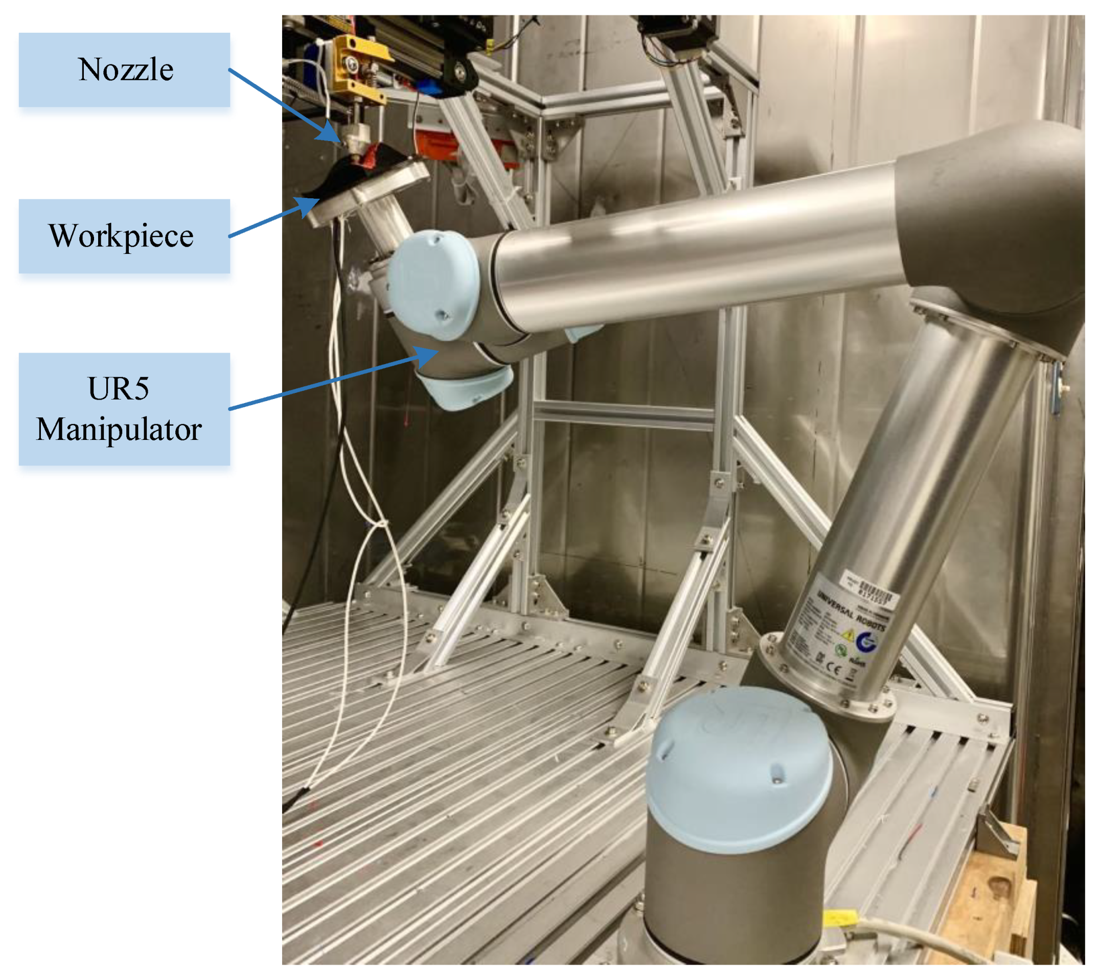
As the self-rotation of the nozzle-axis is irrelevant to printing, a general printing task normally requires five DOFs with 3-DOF for positioning and 2-DOF for identifying the orientation of the nozzle. As a result, when an industrial 6-DOF robotic manipulator is applied for printing, such as the frequently used UR5 manipulator shown in
Figure 4, the extra DOF will result in a functional redundancy in robotic motion planning (for more details about the kinematic redundancy, please refer to [
21,
22,
23]).
By default, the printing path is firstly defined in the WCS. According to the geometry information of the workpiece, each NL point on the printing path can be expressed as a vector
defining its point location and the associated orientation. In addition, another two frames are introduced to specify the coordinate transformation: the nozzle coordinate system (NCS) and the base coordinate system (BCS) of the manipulator. As shown in
Figure 4, the NCS is defined at the tip of the nozzle, while the WCS is fixed on the end-effector of the manipulator. Since the central point of the nozzle is taken as the origin of NCS and its
-axis is set exactly coincident with the NL orientation (see the auxiliary graph in
Figure 4), the NCS can thus be expressed as
where the Euler angles
indicate the axle rotation with respect to the WCS. The transformation from WCS to NCS can be identified by a homogeneous transformation matrix
as:
where
() and
() are the standard translation and rotation matrices, respectively. Thanks to the consistency of nozzle orientation defined in the NCS and WCS, a simplified relation between
and (
can be extracted from Equation (3) as:
This relation reveals the fact that the angle parameter in NCS can be arbitrary, which is the cause of kinematic redundancy.
To facilitate the kinematic analysis of robot manipulators, the configuration Θ is used to denote the joint variables of the manipulator with respect to BCS. Now that the redundant
implies infinite joint solutions for the end-effector posture, it can be capitalized for a better planning of the joint configuration under certain specific constraints, e.g., to avoid the singularities. As it is well known in robotic path planning, a good path should not only bypass any singularities but also preferably stay away from them, as near a singular configuration, even a small change in the operational space on the printing path would cause a drastic change in the joint motion in the configuration space in order to maintain the desired trajectory [
16]. Therefore, singularity avoidance is chosen by us as one objective to optimize the kinematic performance. To evaluate a singular state of manipulator configuration, Huo and Baron [
24] proposed a manipulation performance index
, called the parameter of singularity (PS), which is a function of angle
and defined as:
where scalars
are the eigenvalues of the geometric Jacobian matrix sorted in the descending order (more details can be found in [
24]). As
varies with angle
, different configurations will lead to different
’s, and the smaller it is, the better conditioning is the manipulator. Therefore, this measure is chosen by us as the criterion for evaluating and, thus, to effectively avoid the singularities. For all possible configurations, the optimization objective aims at minimizing
to physically place the manipulator as far away as possible from any singular state. Specifically, for a single nozzle posture
defined by its position and orientation, a minimized singularity parameter
can be resolved by solving the minimization problem of the following form:
With
identifying the posture of the end-effector
, we can then finally determine the joint configuration
expressed as a set of six joint angles
by the inverse kinematic transformation (IKT) which is a standard computation procedure in robotics [
25].
2.2.2. Kinematic-Constrained Feed Rate Optimization
For the robotic arm, it is physically constrained by its configuration limits, such as the velocity, acceleration and jerk, which are also called the kinematic capacities. To make the robotic arm operate within its kinematic capacities, motion planning considering the kinematic constraints is important, as a stable end-effector with less vibration is crucial for maintaining a smooth and steady nozzle path. For this purpose, the feed rate, i.e., the sweeping speed of the nozzle tip, should be adjusted/controlled carefully to assure that the motion of robotic manipulator is always within its kinematic capacities.
Specifically, to calculate the joint velocity, acceleration and jerk at a single NL point that lies on an NL curve, the continuous feed rate scheduling problem is first converted to a discrete form by sampling the NL curve into equal-spaced sample points. The arc length between each pair of adjacent sample points is approximated by the chord-length
, which is assumed to be sufficiently small. As aforementioned, for any sample NL point
p, its corresponding configuration can be determined by choosing from appropriate angle parameters according to the stipulated secondary criterion: the singularity avoidance. Let
and
be the preceding and succeeding sample points of
p, respectively, and
their corresponding joint configurations, with each configuration represented by six joint angles (
. Referring to [
26], for each point
, its velocity, acceleration and jerk of those corresponding six joints can be numerically derived by:
where
is the feed rate at point
, which is a function of feed direction
θ with respect to the local geometry, and
denotes the chord-length. To satisfy the physical constraints, each joint should be constrained by its maximum values:
where
,
denote respectively the maximum (angular) velocity, acceleration, and jerk of joint
, all of which are constants. Combining Equation (7) with Equation (8), the maximized feed rate under the velocity, acceleration and jerk constraints along feed direction
can then be identified, which will be denoted as
,
, and
respectively. Naturally, the most restrictive of the above three should be regarded as the maximum allowed feed rate at
p in the
direction, i.e.,
:
By now, the most conservative feed rate under the physical constraints of the robotic manipulator considering the singularity-avoidance has been established. Furthermore, combining with the effective printing width constraint (
Section 2.1), we next proposed an indicator of printing efficiency that will synthesize on both these two feed-direction sensitive functions.
2.3. Indicator-Determined Preferable Feed Direction
From the perspective of printing, as the surface layer to be printed is given with a specific geometry and thickness, it naturally leads to a fixed volume to be filled by the deposited material. Then, if the volume deposited per unit time is larger, a shorter time will be needed to infill this volume. Since the cross-section of a filament is regarded as an ellipse, the printed volume along a single printing path is thus that of an elliptic cylinder. Considering this fact, an indicator named the material deposition rate
is proposed here to evaluate the printing efficiency, which represents the printed volume per unit time. Explicitly,
at any NL point is defined as:
where
h is the thickness of the current printing layer,
is the effective width, and
is the most conservative feed rate determined by the physical constraints and singularity avoidance along the feed direction
.
To construct the indicators of the sample points on the layer surface
S and find out the representative optimal feed directions for the whole surface, we propose a sampling-based strategy. For any sample point on
S, the potential feed direction in the range of
is first discretized into
n equal interval radians, i.e.,
. Assuming that
S is given as a triangulated mesh, its vertices are chosen as the sampling points for evaluation by the proposed indicator and collectively called the sampling point set
. At each sample point
, the effective printing width
and the optimized feed rate
for any
can be found as described in the previous sections. Then, by Equation (10), the material deposition rate on
S is uniquely defined as a continuous scalar function of the feed direction
at point
. However, although there is an optimal feed direction
and the corresponding maximum
for each
, our objective is to find a single feed direction (as associated with a single drive plane) that will maximize the total material deposition rate for the entire
S. For this purpose, the following discrete optimization formula is proposed:
where
denotes the average material deposition rate at
among
m sampling points. The single solution to Equation (11), i.e.,
, will then be taken as the preferred printing direction for the entire layer surface
S. Below, Algorithm 1 gives the pseudo-codes of this procedure for finding angle
.
| Algorithm 1 Optimized feed direction determination |
Input: A triangulated mesh surface with vertices set
Output: Optimized feed angle
//* Refer to Section 2.1 and Section 2.2
1 for and do
2 by Equation (2)
3 by Equation (6)
4 referring to [25]
5 by Equation (9)
6 end
//* Refer to Section 2.3
7 by Equation (10)
8 by Equation (11)
9 return |
With the drive plane direction found (as identified by the single angle from Equation (11)), we next proceed to describe how to generate an iso-planar nozzle path to print the entire S.
3. Optimized Iso-Planar Path Generation
Figure 5 gives an illustration of NL curve generation based on the iso-planar method. Basically, the NL curves
are the intersections between the layer surface
S and a series of parallel driving planes. For each drive plane
Q, it is perpendicular to the plane
and with a normal
in
.
Let
denote these yet-to-be-determined successive drive planes, each inducing an NL path, e.g.,
in
Figure 5, which is sampled into a discrete form. The very first drive plane
is readily defined—it is simply an extreme plane of
S with a normal vector of
. The approximation as introduced in [
6] provides a way to determine the sample density of an NL curve, i.e., the forward step
between any two adjacent points
and
is approximated by the chord length satisfying the chord-error constraint
, which can be explicitly expressed as:
where
is the curvature radius of
S along the direction of
at point
and
is the specified maximal chord-error.
For the feed-material flow, it is achieved by the mechanics of the motor controllers of the 3D printer. In our experiment setting, the motor control of the extrusion system works by using piecewise linear segments to approximate a smooth curve. As shown in
Figure 6, to synchronize the nozzle motion with the material extrusion, the volume-equilibrium between the deposited material and the feed material is used to determine the feed step
. Specifically, this volume equilibrium, of which the left side is the volume of the deposited material from
to
and the right one represents the cylinder volume of feed material from
to
, is given as:
where the nozzle diameter
, the layer thickness
, and the radius of feed material
are user-determined and
is the forward step computed by Equation (12). Accordingly, the feed step of the supplied filament
is fully decided.
As for the nozzle orientation assignment, we enforce that the nozzle axis should align with the surface normal at the NL point, lest the local gouging between the printed layer and the nozzle may occur. In such a way, a single curve containing the nozzle location and the orientation can be well determined.
After the initial
curve is decided, its adjacent path can be expanded accordingly. Akin to carefully controlling the sampling density of an individual NL curve, to uphold the printing quality, the density of NL curves should also be strictly controlled. Let
denote the side-step distance between two arbitrary adjacent drive planes. As discussed in
Section 2.1, each point on an NL curve
has a corresponding
value, even along the same printing direction. To determine the side-step
for the current NL curve, the minimal one
among all the
m sample points on the NL curve will be taken as the most conservative side-step, i.e.,
Starting from the first drive plane
and its corresponding NL curve, by applying Equation (14), we obtained the second drive plane
and its NL curve, then the third
and its NL curve, …., until the last one
and its NL curve when the opposite extreme edge of
S was reached. As the side-step
is adaptively decided, the material deposition becomes more even and regular, which is opposite to the conventional equal-distance side-step approach. Algorithm 2, given below, summarizes this procedure.
| Algorithm 2 Efficiency optimized iso-planar printing path generation |
Input: (1) A triangulated mesh surface with vertices set
(2) Drive planes
(3) Optimized feed direction
Output: The computed NL paths (both nozzle location p and orientation n)
1 for do
2
//* Single NL path determination
3 for do
4
5 by Equation (12)
6 if
7
8 else
9
10 end
11
12 end
13
//* Next driving plane with side-step determination
14 by Equation (14)
15
16 end
//* Output all the computed NL paths
17 return |
4. Results and Discussion
To validate the proposed multi-axis nozzle path planning methodology, the prescribed algorithms have been implemented by us using MATLAB. In addition to computer simulation, as shown in
Figure 7, for carrying out physical printing experiments, we built a prototype of a robotic manipulator-based multi-axis FDM printing system which integrates a popular 6-DOF UR5 robotic manipulator with a nozzle extruder. The processing parameters used in the experiments are listed in the following
Table 1:
In total, there are four printing surfaces selected for testing the proposed algorithms, i.e., a saddle surface (
Figure 8a), a bicycle seat surface (
Figure 8b), and two freeform surfaces with concave and convex regions (
Figure 8c,d). For these test surfaces, which are originally given in CAD NURBs format, they are first discretized into triangulated meshes with the help of the software HyperMesh. During the process of triangulation, the specified maximal chord-error
is used as a control variable of point sampling, so to ensure the accuracy of the mesh models. Then, the triangulated meshes as shown in
Figure 8 are used as the input to the proposed algorithms, and the vertices of the meshes are used to calculate the material deposition rate.
After running Algorithm 1 using the parameters of
Table 1, the
among different feed angle
for the four test models are computed and displayed in
Figure 9, with both the optimized angle and its corresponding deposition rate annotated. For
S1, as shown in
Figure 9a, the indicator indicates several distinct local maxima, and the best of which occurs at
with a maximum
mm
3/s. For the second model,
S2 shown in
Figure 9b, since the surface is symmetric about the
x-axis, the indicator
shows a symmetry about
=
(barring the inaccuracy due to the meshing and numerical errors), and a global maximum
is identified. For the two freeform surfaces
and
(
Figure 9c,d), the optimized angles are
and
, respectively, while there is little difference between the deposition rates with various angles, especially for
. This is because, for these two surfaces, for any direction, the intersection curve between the corresponding drive plane and the surface always has portions of large curvature, which makes it difficult for Algorithm 1 to find a distinguishingly better direction angle.
With the optimal angle
found by Algorithm 1, Algorithm 2 (see
Section 3) is then executed, which iteratively generates the NL paths for the given curved surfaces. Finally, these NL curves are connected in a zig-zag pattern to form the continuous printing paths, as shown in
Figure 10.
Among the four surface models, two are selected further for physical printing tests, i.e., the saddle surface
and the bicycle seat surface
. For these two surfaces, the printing paths generated from Algorithm 2 are first converted into the G-codes of the homebuilt multi-axis FDM printing system and then executed. For comparison purposes, a benchmark printing path is also executed for each of the two surfaces. To facilitate the printing, a support-base is pre-fabricated beforehand for each of the two surfaces.
Figure 11 displays some snapshots of the two printing processes, wherein the red surfaces are the partially printed layers while the support-bases are in black.
Figure 12 displays the final printed surfaces
and
, respectively, using both ours and the benchmarking method. In
Figure 12a,d which show the printed parts using the proposed method, the black lines mark the optimized feed directions of the printing paths, with the optimized angles tagged by
, and
denoting the side step between the two involved adjacent NL curves. For a more detailed examination, the regions circled in green are magnified, as shown
Figure 12b,e, respectively. As a whole, the re-solidified material is well deposited and evenly arranged onto the support-base, which owes much to the adaptive determination of both the side step and forward step. However, the zoomed pictures also indicate that over-extrusion or under-extrusion of the deposited material may not be fully eliminated, for which we offer the following explanations. First, as aforementioned in
Section 3, the motor control of the extrusion system in our setup is based on the piecewise linear approximation of a smooth NL curve, which may induce certain inaccuracy. Secondly, the current adaptive side-step decision is based on a simplified ellipse model, which may incur inaccuracy in the actual amount of the deposited material. Thirdly, the controller of the UR5 arm may automatically alter the scheduled feed rate during the printing process whenever it deems necessary, which also affects the deposition rate. Regarding the comparison,
Figure 12c,f shows photos of the printed
S1 and
S2 using the benchmarking method which is still the iso-planar method except that the drive plane direction is arbitrary. Note that, except for the different directions of the drive planes, both the proposed method and the benchmarking method use the identical method to determine the side-step
and the feed rate. Therefore, as the photos show, both the proposed method and the benchmarking method are similar in terms of printing quality.
The real printing time and the total printing length have been recorded by the controller of our homebuilt multi-axis printer and they are listed in
Table 2. The results indicate that the proposed method has reduced the total printing time against the benchmarking method by 10.8% and 35.5%, respectively, for
and
. For these improvements, we offer several plausible explanations. The first and also the primary one is that, by considering the effective printing volume as a global optimization objective, the proposed method has effectively determined an optimized drive plane angle to minimize the total printing time. Secondly, as revealed by the total path length data shown in
Table 2, the printing paths generated by the proposed method are shorter than that by the benchmark method, which is chiefly due to the fact that, as the proposed indicator involves the effective printing width which is related to the local curvature of the printing layer, a higher deposition rate is always sought locally, which in turn will reduce the total printing length (since the total printing volume is fixed). Finally, it is noted that the proposed indicator considers not only the local curvature of the printing layer but also the kinematic capacities of the robot arm. Altogether, these factors contribute to a significant improvement in printing efficiency by the proposed method.
5. Conclusions
The primary objective of this paper is to develop a multi-axis printing path generation algorithm for an arbitrary curved freeform layer, such that the kinematic capacities of the 6-DOF robot arm (which enables the rotation of the nozzle) can be fully utilized while the required printing quality in specific tolerance is upheld. Our solution is to first establish a printing efficiency indicator that considers both the local geometry of the layer surface and the kinematic capacities of the robot arm. The classic iso-planar method is then adopted to generate a printing path; wherein, the normal of the parallel drive planes is exactly the one that globally maximizes the efficiency indicator and the side-step between adjacent drive planes is adaptively adjusted to maintain the required printing quality. We have carried out physical printing experiments of the proposed method and compared with some benchmark printing paths, and the preliminary results give a positive confirmation of the proposed method.
Future work will focus on three topics. First, while the iso-planar type of printing path is prevailing in practice, other types do exist, such as the parallel-contour type and its various variations. Thus, it is natural to inquire if similar ideas of this paper can also be applied or extended to some of those non-iso-planar printing path patterns. Secondly, at present, the nozzle orientation is mechanically assigned—it is simply aligned with the surface normal at the NL point. Since the change of the nozzle orientation has a huge impact on the joint motions of the robot arm, it is plausible to include the nozzle orientation as a variable to optimize, tending to all the constraints such as collision-avoidance. Finally, our proposed printing path generation method is restricted to a given printing layer, while the printing layers are generated independently of how the printing paths are generated on them. Aiming at further improving the printing efficiency, it will be interesting to see if these two processes can be coupled together.


