Article

Simulation Study on Single-Lip Deep Hole Drilling Using Design of Experiments

by
Daniel Fandiño
1,
Vinzenz Guski
1,*,
Robert Wegert
2,
Hans-Christian Möhring
2 and
Siegfried Schmauder
1
1
Institute for Materials Testing, Materials Science and Strength of Materials, University of Stuttgart, 70569 Stuttgart, Germany
2
Institute for Machine Tools, University of Stuttgart, 70174 Stuttgart, Germany
*
Author to whom correspondence should be addressed.
J. Manuf. Mater. Process. 2021, 5(2), 44; https://doi.org/10.3390/jmmp5020044
Submission received: 31 March 2021 / Revised: 27 April 2021 / Accepted: 30 April 2021 / Published: 4 May 2021
(This article belongs to the Special Issue Surface Integrity in Machining and Post-processing)

Abstract

:
Single-lip deep hole drilling (SLD) is characterized by a high surface quality and compressive residual stress in the subsurface of the drill hole. These properties are strongly dependent on the cutting parameters of the SLD process and the actual geometry of the insert and the guide pads. In the present work, full 3D FE simulations of the SLD process were carried out to analyze the thermo-mechanical as-is state in the drilling contact zone by evaluating the feed force, the temperature, as well as the residual stress in the drill hole subsurface. An extensive simulation study was conducted on the effect of the process parameters on the properties using design of experiments (DoE). For the simulations, the Johnson–Cook (JC) constitutive law and the element elimination technique (EET) were applied to represent the material behavior of the workpiece, including chip formation. In-process measurements as well as results from the hole-drilling method to determine residual stresses were conducted to verify the numerical results. By means of DoE and analysis of variance (ANOVA), regression models were developed to describe the effect of the feed rate, cutting speed, and guide pad height on the temperature, feed force, and residual stress in the subsurface.

1. Introduction

The global drilling machine market has been growing for years. Based on the application, the whole market is classified into different drilling machines. Among these, the deep hole drilling machine sector is anticipated to dominate the market [1]. The significant growth rate of deep hole drilling machines, which is a method of drilling holes of a high length-to-diameter ratio, is due to the increasing demand for drilling deep holes in a wide variety of machines and equipment across aerospace, automotive, military, defense, as well as oil and gas industries. Another aspect that characterizes deep hole drilling processes is the high surface quality and the evacuation of chips during the operation, which is carried out by means of a cooling lubricant. In this way, the shape and size of the chip plays an important role in the performance of the process. Regarding conventional deep hole drilling techniques, single-lip deep hole drilling (SLD) and BTA deep hole drilling are distinguished. SLD is used for small-diameter machining in the range of 0.5–40 mm, for example, for the production of diesel fuel injectors in the automotive industry [2]. To prevent the components from failing, the formation of microcracks in the component surfaces must be avoided. Crack formation can be prevented with high surface quality and the targeted introduction of compressive residual stresses [3]. Improvements in deep hole drilling technology are driven by better quality and reduced cost. Increasing the material removal rate and increasing the tool life without compromising surface integrity are two ways of reducing costs. In this context, understanding the interaction of process parameters, such as the feed or the cutting speed, or geometrical parameters of the cutting insert or the guide pads with the resulting thermo-mechanical state of the process and the surface of the bore hole is essential. One way to achieve this is the application of modeling techniques. The finite element method (FEM) is the most widely used modeling tool in mechanical engineering. This is recognized by the vast number of publications on this topic as well as the modeling novelties introduced. However, most of the numerical investigations simplify the complex machining process by using FE models of orthogonal cutting [4,5,6,7,8] or by modeling only a part of the cutting insert [9,10]. The current work presents a full 3D simulation of the SLD process with a complete drill head tip using the commercial FEM solver ABAQUS 2018. As a result, information on the shape and size of the generated chip, the temperature, the force in the feed direction, and the induction of residual stresses was obtained.
The design-of-experiment (DoE) approach is a powerful tool to identify in-process dependencies of the process parameters with the resulting quantities. Especially, in the field of production engineering, many applications exist using DoE due to the high complexity of the processes defining several process parameters to obtain a high product quality reliably [11]. Based on such investigations, the combination of simulations with a DoE approach is the next step, intuitively. However, due to the high computational effort performing drilling simulations, few studies have been performed with such a combination [12,13]. To the best of the authors’ knowledge, it is the first time that SLD process simulation studies on full 3D FE models are combined with a DoE approach to analyze the results. The DoE approach delivers a clear dependency of the process parameters on the thermo-mechanical state but a minor effect of the geometrical parameters, such as the guide pad height, on the temperature and the feed force. However, this parameter affects the residual stress in the subsurface strongly. The overall objective using the DoE approach in this study is the development of regression models to be implemented in the drilling process control. In combination with tool-side sensors, the regression models will be employed to forecast resulting subsurface properties, such as residual stress. Finally, this provides an opportunity to adjust the process parameters during the process if the targeted subsurface properties are not reached [14].
For the development of the regression models in this study, in the second section, Materials and Methods, the experimental setup and results are described. In addition, the FE models and the DoE approach are presented in detail. In the third section, Results, the results of an FE simulation are shown, exemplarily, and the results of analysis of variance (ANOVA) studies for the response quantities feed force, maximum temperature in the drill head, and residual stress are presented. Finally, the presented work is concluded in the last section.

2. Materials and Methods

2.1. SLD Experiments

Experimental tests on the SLD process were performed at IfW (Stuttgart University). Parameters such as temperature in the tool and in the workpiece, feed force, and residual stresses were investigated. The experimental setup is shown schematically in Figure 1a. This setup is part of a more complex experimental framework, which is not part of the present study [10,14,15]. The experimental investigations were performed on the deep hole drilling machine Mö-TM-HF-16-2-S (Walter Möck GmbH, Sonnenbühl, Germany). The feed force and the drilling torque were measured with the KISTLER 9125A measuring system (Kistler Group, Winterthur, Switzerland). The employed rotational dynamometer measures the feed force and the drilling torque with a frequency of 4 kHz and possesses a linearity of ≤±1% FSO. A thermography system is applied to measure the temperature at the cutting edge. The thermographic camera VarioCAM hr (InfraTec GmbH, Dresden, Germany) is positioned on the backside of the workpiece. This setup obtains the surface temperature of the component without contact [10].
Due to the limitations with using a thermography system for detecting the temperature evolution during drilling, the experimental setup was improved. Here, the tool was firmly clamped in a vice. The workpiece, however, was clamped in a KISTLER 9125A rotary dynamometer in the spindle; thus, the feed force and the drilling torque were measured on the workpiece side. The cooling lubricant supply of the tool was realized via a specially manufactured adapter. The connection for the volume flow measurement and the pressure measurement were integrated into the adapter. Usually, the cooling lubricant is supplied via the spindle. In addition, positive temperature coefficient (PTC) temperature sensors were positioned in the tool underneath the insert. For the wiring of the 11 PTC sensors, PTFE-insulated copper wires were used. Connecting the sensors to the measuring card PXIe-4357, the wires were led over the cooling channel of the shank of the drill. Then the resistance change was detected, converted into temperatures using LabVIEW software, and finally evaluated [14].
In the framework of this study, the results of the previous setup including the thermography system were employed for comparison purposes with the simulation results. The specimens are cylindrical workpieces with an outer diameter of 25 mm and lengths from 5 mm up to 100 mm and made of 42CrMo4 tempered and quenched steel. Usually, the samples were prepared with a pilot hole with a depth of 1.5× diameter. First, the drilling test was performed under dry conditions to create a reference for the FE simulations. Pressurized air is used to carry out the chip evacuation. The cutting speed was vc = 80 m/min and the feed per tooth f = 0.042 mm/rev. Each drilling test was repeated three times [10].
The simulated tool is a single-lip deep drill with a changeable insert and guide pads (Gühring AG, Albstadt-Ebingen, Germany). The original part is 644 mm long and has a diameter of 18 mm. It consists of four changeable guide pads, as shown in Figure 1b. The insert and the guide pads are made of hard metal K40 with a TiN coating.
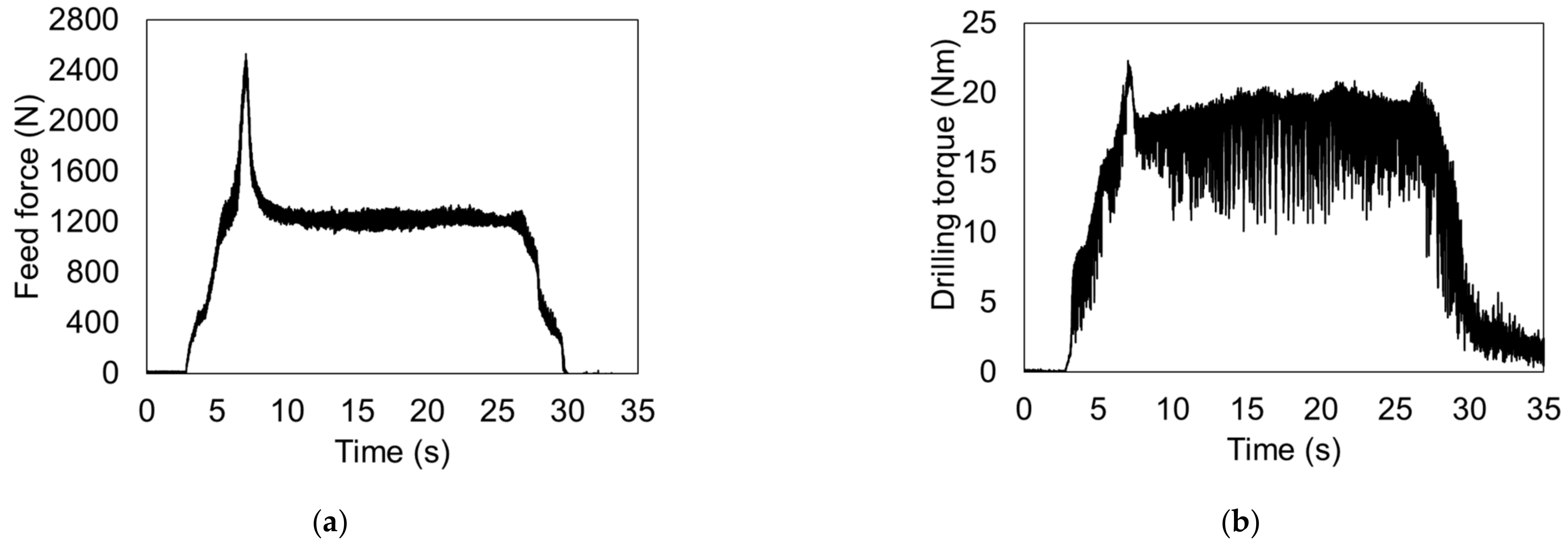
In the drilling experiments, a characteristic evolution of the feed force as well as the drilling torque were observed, with a steep increase in the quantities after the contact of the drill head with the workpiece (Figure 2). Both quantities reach a maximum, which were up to 3 kN for the feed force and up to 50 Nm for the drilling torque within the whole test series, a few seconds after the beginning of the process. Behind the peak, a plateau is formed with steady-state conditions until the samples are drilled through. The results in Figure 2 were obtained from a cylindrical sample with a length of 20 mm and an outer diameter of 25 mm. Here, the feed force reaches a maximum of 2.5 kN and steady-state conditions with a constant feed force of 1.3 kN, whereas a maximum drilling torque of 22 Nm and steady-state conditions with a torque of 19 Nm were obtained. Due to the dynamics of the process, leading to vibrations, both curves show a scatter, which is pronounced in the curve of the drilling torque (see Figure 2b) [10].
In addition to the mechanical conditions, the temperature was measured with a thermography system. For each measurement, the frame at the breakthrough of the driller was evaluated and the maximum temperature determined. At the beginning of the measurements, the emissivity was determined by a calibration measurement with a value of 0.44. Figure 3a shows the resulting frame of the measurement on the sample with a length of 20 mm. As indicated by the light-magenta color, the maximum temperature of 600 °C was observed on the outer edge of the cutting insert. This observation was reproduced by the other measurements. The determined temperature peaks at the drill exit for all the samples with lengths between 5 and 50 mm are summarized in Figure 3b. The linear regression line indicates a continuous increase in the temperature with increasing drilling depth. A similar correlation was obtained for the mechanical quantities. The maximum temperature starts close to 600 °C for a drilling depth of 5 mm. Finally, a maximum temperature up to 775 °C is obtained for a drilling depth of 50 mm [10].

2.2. SLD Simulation: FEM

The CAD of the SLD tool was obtained from the manufacturer. To simplify the simulation, only the drill head tip was taken into account, which has a length of 9.84 mm of the whole tool. The shortened CAD of the SLD tool for the simulation is shown in Figure 1b. The shortening of the tool also means that only two of the four guide pads are going to be simulated. In addition, the remaining CAD was adjusted to homogenize the applied discretization by merging the removable parts (the two guide pads and the insert) with the tool shank and removing the screw that tightens the insert with the tool shank. However, to simulate the heat transfer from the insert into the screw, the hole was filled. To simulate the workpiece to be cut, a cylindrical part was created with a diameter of 25 mm and a length of 5 mm.

2.2.1. Constitutive Law

The modeling of the materials plays an important role in the results of the simulation. Incorrect input data can produce errors during the simulation or incoherent results. The selected material for the workpiece is DIN 42CrMo4 (AISI 4140) low-alloy steel. This material has been widely used for automotive driving elements such as crankshafts or steering components [16], as well as in the production of common rails for injection systems. For the simulation of the tool material, tungsten carbide with 15% cobalt as a metal binder was selected.
  • Workpiece material
The elastic inputs can be derived from the stress–strain curves of tensile tests. Since heat generation between the tool and the workpiece is expected due to plastic deformation and friction, temperature-dependent data are used. Moreover, isotropic elastic properties are considered. A Poisson’s ratio ν of 0.3 is assumed, independent of temperature. Table 1 shows the input data for the temperature-dependent elastic properties.
To model the plastic behavior of the workpiece, the Johnson–Cook (JC) constitutive equation is implemented [17]. During the drilling process, the workpiece material is treated with high levels of strain, strain rate and temperature. For this reason, it is important to take these dependencies under consideration in order to model the flow stress σ of the material more precisely. This equation is commonly used when modeling orthogonal cutting in FEM simulations [4,5,6,7]. The JC constitutive model is presented in Equation (1) [18].
σ = A + B ε n 1 + C l n ε ˙ ε ˙ 0 1 T T a T m T a m
where A, B, C, n, and m are the five JC parameters, which are material dependent; ε is the actual plastic strain; ε ˙ and ε ˙ 0 are the actual strain rate and the reference strain rate, respectively; Tm is the melting temperature; and Ta is the ambient temperature. The input values are given in Table 2.
To simulate the damage initiation, the Johnson–Cook criterion is used. It is a special case of the ductile damage criterion model. The model represents the damage caused by nucleation, growth, and coalescence of voids in ductile materials. The equivalent plastic strain induced by the damage is considered as a function of stress triaxiality and strain rate [19]. This model is compatible with the JC plasticity model. The equation of the model is expressed as [20,21]
ε ¯ D p l = d 1 + d 2 e d 3 λ 1 + d 4 l n ε ¯ ˙ p l ε ˙ 0 1 + d 5 T *   with   T * = T T a T m T a
where d1d5 are failure parameters, λ is the stress triaxiality, ε ˙ 0 is the reference strain rate, and T* is the dimensionless temperature. The failure parameters d1d5 were determined by means of a sensitivity analysis in order to produce more realistic chip forms. In Table 3, the values for the JC damage initiation model are listed.
After damage initiation, the stress–strain relationship does not describe the material’s behavior in a precise way. Therefore, a damage evolution criterion is defined in combination with the damage initiation. In the damage evolution criterion for ductile metals, the damage is described by the progressive degradation of the material stiffness, leading to material failure [19]. To drive the evolution of damage after damage initiation, a critical displacement is defined. Damage evolution with a critical displacement at failure of 0.0001 mm is assumed. To simulate how the workpiece material is affected by the temperature, thermo-physical properties, such as the thermal expansion coefficient, thermal conductivity, and specific heat, are defined. The temperature-dependent data for the simulation are presented in Table 4.
ABAQUS allows the introduction of heat generation caused by mechanical dissipation associated with plastic straining. This feature is applied for deep hole drilling process simulations. Thus, the inelastic heat option is activated with a value of 0.9, which means that 90% of the inelastic dissipation is converted into heat. The solver requires a constant density ρ value, which was set in the simulations to 7850 kg/m3. ABAQUS also permits the deletion of elements using state variables [19]. Therefore, one solution-dependent state variable and one variable controlling the element deletion mechanism are activated to represent material failure.
  • Tool material
The tool material is considered isotropic, and it is assumed that no plasticity in the tool occurs during the drilling process. In addition, wear is not considered to reduce the complexity of the model. Thus, damage initiation and damage evolution are not applied in the tool. Moreover, it is assumed that temperature has no considerable influence on the tool and no temperature-dependent data are required. Table 5 shows the input data for the tool material.

2.2.2. Step Definition

The time integration scheme chosen for the simulation is explicit, since it is able to solve problems faster with different non-linearity sources. The coupling between a dynamic and a thermal stress analysis and the definition of the contact properties are more efficient in explicit simulations compared to implicit simulations [24]. Another important aspect of explicit procedures is that the size of the increment depends on the element dimensions and material properties [25]. To simulate the highly dynamic and unsteady single-lip deep hole drilling process, a coupled thermal stress analysis using an explicit integration was conducted. A mass scaling factor of 100 was used, which increases artificially the mass of the elements of the mesh to increase the time increment and thus reduces the computational time without affecting the results in a sensitive way.

2.2.3. Interaction Properties

For this simulation, it is important to consider the mechanical and thermal contact properties. To define the mechanical contact, a contact hard pressure-overclosure relationship and frictional behavior are considered. Likewise, heat generation due to friction and thermal conductance are taken into account to define thermal contact properties. For this simulation, the isotropic Coulomb friction model is used with a friction coefficient μ of 0.32 [9].
Heat generation is simulated using the parameters predefined by ABAQUS. This means that all energy dissipated caused by friction is converted to heat and is equally distributed between the tool and the workpiece. Thermal conductance between the surfaces is modeled defining the gap conductance. ABAQUS is applied to compute the conductive heat transfer between the contact surfaces according to [19]:
q = k T A T B
where q is the heat flux per unit area crossing the interface from point A on one surface to point B on the other one, k is the gap conductance, and T A and T B are the temperatures of these two points on the surfaces. The gap conductance is defined with a tabular clearance dependency but only to establish a constant value. The assumed value for k is 45.000 W/(m2 K). When creating the interaction, the surface of the tool is defined as the master surface and the set of nodes of the workpiece as the slave surface. The penalty contact method is selected as a mechanical constraint. This method produces less stringent enforcement of contact constraints compared with kinematic contact. However, it permits the definition of more general types of contact, for example, multiple contacts per node [19]. Finally, the finite sliding setting is chosen, which allows any arbitrary motion of the surfaces.
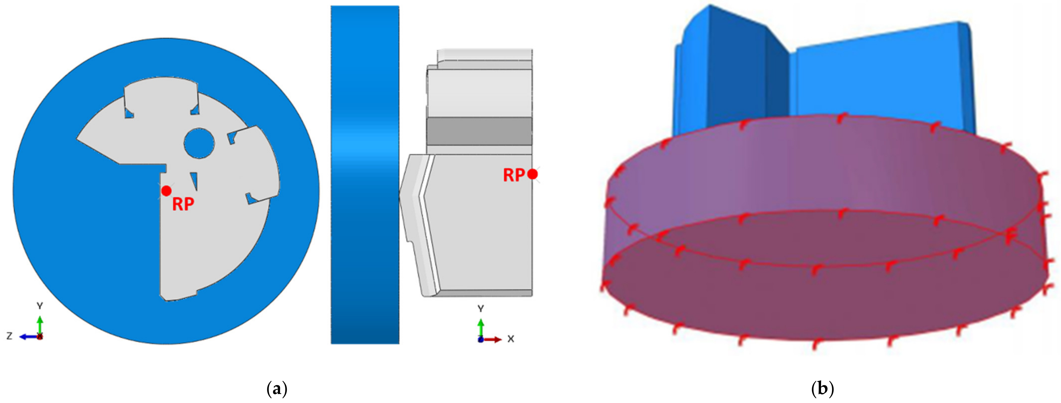
In addition to the interaction properties, a rigid body constraint between the tool and a reference point is set. The reference point is located on the axis of rotation of the tool surface (see Figure 4a). This constraint is added to enter the boundary conditions in a simple way later, that is, the feed rate and the rotation speed of the tool, which are defined through this reference point.

2.2.4. Boundary Conditions

In the simulation of the deep drilling process, boundary conditions are used to specify the feed rate and rotation speed of the cutting tool. In addition, the movement of the workpiece is also restricted to simulate the drilling process. To simulate the movement of the tool, a boundary condition is first defined that allows displacement and rotation only on the longitudinal axis of the tool. The movement in the other axes is restricted. Then another boundary condition is created, which allows one to specify angular velocities and speeds. These boundary conditions are applied to the node, which is defined as the reference point, and is linked to a rigid body constraint in the previous step (see Figure 4). This guarantees that the tool will move according to the boundary conditions defined in the reference point.

2.2.5. Discretization

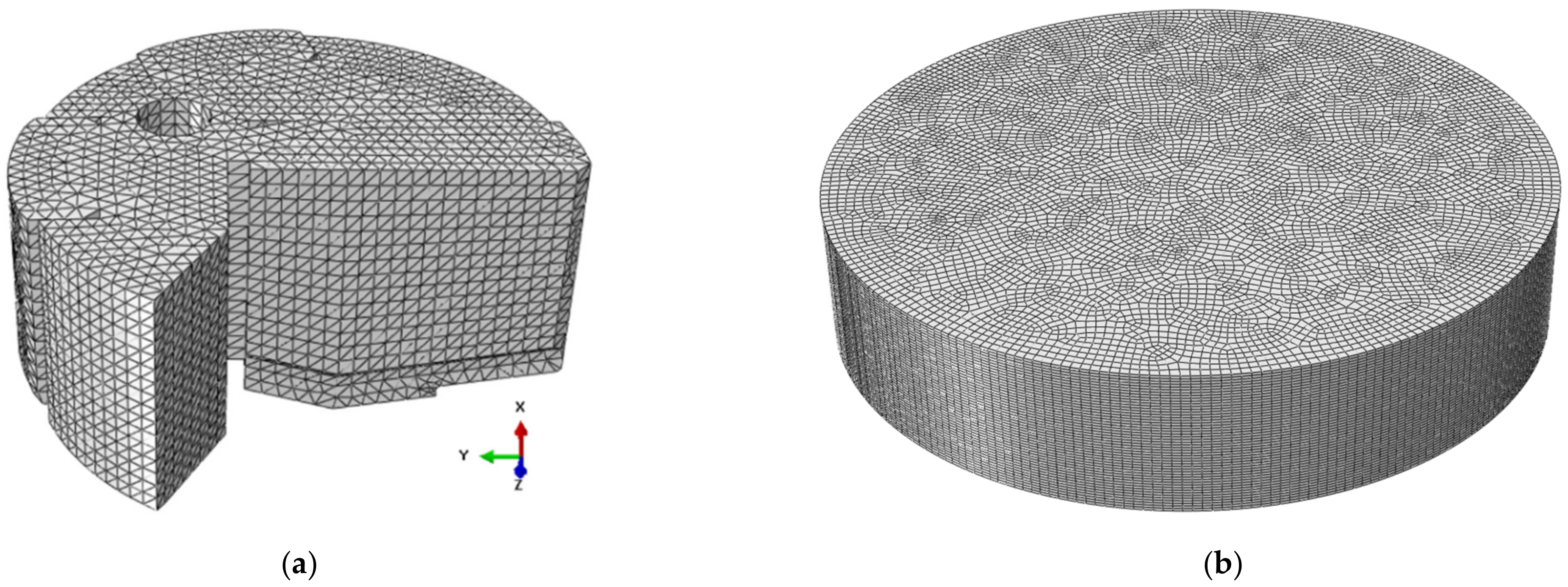
For the SLD simulation, a constant mesh density is used for both the workpiece and the drill head. On the one hand, the size of the workpiece is just enough for the drilling process to be carried out. Thus, the application of refining techniques is not required. On the other hand, the complex shape of the drill head makes it necessary to use a fine mesh to achieve the simulation without errors. Linear four-node tetrahedral elements with coupled temperature displacement and an explicit time integration scheme (C3D4T) are used for meshing the drill head. A global size of 0.5 mm is selected, thus generating 60,867 elements (see Figure 5a). For the workpiece, hexahedral elements with eight nodes (C3D8RT) are employed. These elements are suitable for a coupled temperature-displacement analysis with explicit time integration. The reduced integration function with hourglass control and the distortion control feature are activated. It was decided to work with a size of 0.3 × 0.1 mm, thus generating 348,700 elements in the workpiece (see Figure 5b). The implementation of finer meshes means a higher computing time, which would exceed the time limits established for this investigation.

2.3. SLD Simulation: Design of Experiments

To investigate the influence of the process variables on the SLD simulation, a general full factorial experiment is designed. It consists of an experiment with all combinations of factors. This enables a complete and systematical investigation of the interactions between influences of factors to identify the significant ones [11]. These interactions are investigated by means of analysis of variance (ANOVA) for the main effects, interactions, and fitting models. The objective of ANOVA is to generate mathematical relations to predict responses when cutting conditions are subjected to changes. In this study, a linear fitting model was used as a predictor to optimize the temperature or the residual stress with a confidence level of 95. To carry out ANOVA, the statistical analysis software Minitab 2018 is used. Minitab uses the adjusted mean squares (Adj MS), the adjusted sum of squares (Adj SS), and the F-value to calculate the p-value, which is a probability that measures the evidence against the null hypothesis. The null hypothesis of a main effect is that the mean response for all factor levels is equal, while for an interaction, the mean response for the level of one factor does not depend on the value of the other factor level. To determine whether each main effect and the interaction effect are statistically significant, the p-value for each term is compared to the significance level. The significance level is denoted by α and is calculated as (1 – confidence level). If the p-value is greater than the significance level, the effect is not statistically significant. However, if the p-value is less than or equal to the significance level, then the effect is statistically significant. To identify visually the significant effects, a Pareto chart for standardized effects is created. The Pareto chart plots the absolute values of the standardized effects from the largest effect to the smallest effect. The chart also shows a reference line to indicate which effects are statistically significant. The reference line depends on the significance level α. Bars that cross the reference line are statistically significant. The applied regression equation with three factors and their interaction with each other can be written as the following expression:
Y = x 0 + x A i A + x B B + x C C + x A B i A B + x A C i A C + x B C B C
where xA/B/Ci are the determined coefficients and A, B, and C are the factors according to the level i.
In the present work, the influence of the three different parameters guide pad height, feed rate, and cutting speed, which are called factors, on the temperature, feed force, and the residual stress, which are called responses, was analyzed. The number of factors in combination with the number of different values of each factor, which are called levels, determine the total number of trial runs. Here, three guide pad heights, two feed rates, and two cutting speeds were applied. This led to a total number of 12 runs. Table 6 shows the designed experiment for the simulation. The guide pad height hGP refers to the distance between the circle formed by the shank and the circle formed by the drill head, as shown in Figure 6a. A rectangular platform below the guide pad was created to control the height. A height of 0.85 mm was chosen instead of the middle height 0.75 mm because of the minimum platform size required for a mesh without poor elements.
Normally, the feed rate fz is much lower than that selected. Simulating low feed rates means longer simulation times, which are not realistic within the time frame of this research. Therefore, high speeds are selected, and then the results are compared with the experiment by means of extrapolations. Due to the necessity of few complete tool rotations leading to full contact of the guide pads with the workpiece to be able to investigate the effect of the guide pad heights on the residual stress, the cutting speed vc exceeds the applied values in the experiment, too. The designed experiment generates an experiment with 12 runs.

3. Results

3.1. SLD Simulations

The FE simulations of the highly dynamic and unsteady-state SLD process were conducted with the commercial solver ABAQUS with an explicit simulation scheme. According to the defined process parameters in the design-of-experiment approach in Table 6, the simulations were repeated 12 times. To explain the simulation results more in detail, the results of the simulation with a feed of 0.64 mm/rev and a cutting speed of 427.5 m/min are presented in this section, exemplarily.

3.1.1. Chip Formation

As the drill head engages the workpiece, the material directly ahead of the insert is deformed and sheared. The deformed material then breaks and flows into the space above the insert in the form of a chip. In other words, the chip-forming process occurs by plastic deformation and shearing. Information about the chip form is important to predict the machinability of the workpiece material. A short breaking chip is preferred because it does not affect the drilled surface and can be easily evacuated. Exemplarily, the chip formation is illustrated in Figure 6b for the following drilling conditions: guide pad height of 0.5 mm, a feed of 0.64 mm/rev, and a cutting speed of 427.5 m/min. Figure 7a shows a lateral and a front view of the formed chip in the preview illustration. The chip has a conical spiral shape, with a base smaller than the height. The guide pad height did not significantly affect the shape or size of the formed chip. By increasing the feed rate from 40 to 80 mm/s, a smaller chip is obtained, which does not coil completely. The proportions remain the same, with a smaller base cone than height. As for the increase in cutting speed, this causes the formation of a chip with an even smaller cone base. Both, higher feed rates and higher rotation speeds, produce short chips, which are easily managed and evacuated in SLD applications. The chips retain the greatest amount of heat generated during the drilling process [26]. Large chips that cannot be removed make it difficult for the cooling lubricant to cool the process.
During the experiment, mainly two types of chips are formed, a short one with a conical shape and a long one with an accordion shape. The first is known as a spiral chip and the second as a tangled chip. Figure 7b shows a photo of the chips. The model successfully simulates one of the two types of formed chips in the experiment, this being the spiral chip. The chips formed in the experiment have a size similar to the simulated chips. The only noticeable difference is that the chips from the experiment have in some cases a greater cone base than height. By simulating slightly deeper holes, chips could also form with this ratio. To simulate the other chip type (tangled), the simulation of deeper holes would be required. This is currently unfeasible due to the drastic increase in simulation time.

3.1.2. Temperature Evolution

First, the evolution of the temperature in the drill head was analyzed using the following cutting conditions: a feed of 0.64 mm/rev and a cutting speed of 427.5 m/min (see Figure 8). At the beginning, the temperature in the cutting edge increases as the insert drills into the workpiece. Once the drill head tip penetrates the workpiece completely, the heat is concentrated on the front surface of the drill head tip. At the end of the simulation, a maximum temperature of 1466 K in the succeeding guide pad is reached, as shown in Figure 8. To be able to compare the temperature with thermography data, even the maximum temperature at the cutting edge was evaluated. This location is marked in Figure 8a. Here, a maximum temperature of 887 K, which corresponds to 614 °C, is observed.
This temperature at the cutting edge of the insert matches the thermography data in Figure 3a, which shows a maximum temperature in the insert up to 600 °C (white area). A detailed temperature evaluation in the experiments can be found in [10]. The evolution of the temperature at the site of the maximum temperature in the drill head (guide pad) and in the insert is plotted in Figure 8b. At first, the temperature remains constant around room temperature at both positions since they are not yet in contact with the workpiece. After the penetration of the drill head into the workpiece, a steep temperature increase is observed. Then, the temperature remains constant, with fluctuations around 887 K, which can be attributed to the formation of chips. The drill head temperature also increases rapidly upon contact with the workpiece. In contrast to the cutting edge, the temperature shows a stronger upward behavior without significant major fluctuations. The guide pad in the drill head is not in direct contact with the generated chip and reaches a constant maximum temperature of 1466 K, which corresponds to 1193 °C. Due to the experimental setup, the thermography camera reliably detected the temperature distribution in the front surface of the drill head with the cutting edge of the insert. Another observation is that the guide pads, which are positioned behind the insert with respect to the driller axis, cannot be investigated with the thermography system. In further investigations, the application of temperature sensors underneath the guide pads is planned.

3.1.3. Feed Force Evolution

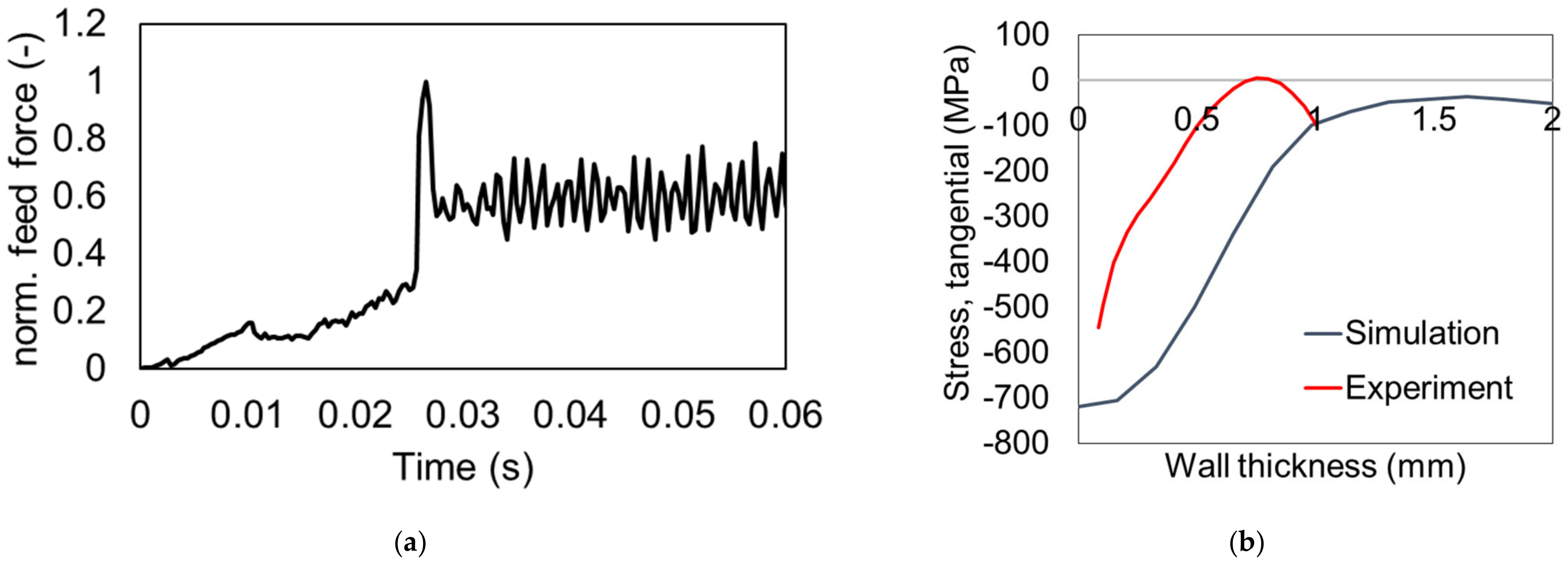
Figure 9a shows the feed force evolution in the simulation. When the simulation begins, the insert is the only part in contact with the workpiece and the drill head acquires the rotation speed and the feed rate instantly. At the beginning, the feed force increases proportionally as the insert drills into the workpiece. The contact area between the insert and the workpiece grows, thus increasing the resistance to drill. Once the drill head comes into contact with the workpiece, the feed force rises exponentially to a maximum value. Thereafter, the feed force decreases and begins to fluctuate around a lower mean value than the previously reached maximum. This means that the feed force reaches a steady state behavior. Due to the accelerated process in the simulation, the feed force overestimates the experimental values (see Figure 2a) [10]. Nevertheless, the shapes of the curves match, which indicates that the mechanisms of the SLD process can be reproduced in the simulation and thus the behavior during the drilling process.

3.1.4. Residual Stress

Residual stresses are formed when a workpiece is subjected to stresses that exceed its elastic limit such that plastic deformation occurs. During SLD, non-uniform plastic deformation occurs, inducing the formation of residual stresses. The objective is to produce deep holes with compressive residual stresses near the borehole surface to avoid the formation of microcracks. The residual stresses in the tangential direction are responsible for preventing the formation of microcracks. For this reason, the formation of residual stresses in the simulation on the workpiece is investigated. To do this, a path from the drilling surface to the outer surface of the workpiece is created. In this way, residual stresses can be measured across the depth of the borehole wall. The tangential residual stress corresponds in this case to the z-axis, which is the stress S33 in ABAQUS. Figure 9b shows a comparison of the residual stresses along the created path from the surface into the borehole wall. Here, compressive residual stresses near the drilling surface are observed. The simulation results are similar to the experimental results, which were obtained by an incremental hole-drilling method according to ASTM E837-20 [27]. A comparable behavior of the residual stresses with respect to the wall thickness is obtained. The calculated values overestimate the experimental results, which can be attributed to the accelerated process in the simulation. Therefore, it can be concluded that the developed model allows one to successfully simulate the formation of residual stresses on the borehole surface qualitatively. In the future, further investigations will focus on the deceleration of the process in the simulation to obtain a better agreement quantitatively.

3.2. SLD Simulation: Design of Experiments

To identify dependencies of parameters such as feed, cutting speed, or guide pad height on the temperature or the feed force in the process, an analysis of variance on the results of 12 runs was carried out. The results are presented in this section.

3.2.1. Temperature

Here, the influence of the cutting conditions on the temperature was analyzed. For this analysis, the temperature at different locations was considered. According to the location at the cutting edge in Figure 8a, the average temperature in the steady state for each run was evaluated. Figure 10a summarizes the temperature results. Two different levels are observed: the temperature in the runs with an odd number is at 610 °C and in the runs with an even number is at 680 °C. This leads to the conclusion that only the cutting speed affects the temperature in the cutting insert. More complex dependencies were obtained for the maximum temperature in the drill head, which is typically located in the guide pad. The maximum temperature in the drill head reached at the end of the simulation is considered. The influence of the cutting conditions on the drill head maximum temperature is shown in Figure 10b.
The lowest temperature of 1025 °C is obtained with hGP = 0.5 mm, fz = 40 mm/s, and vc = 427.5 m/min, and the highest temperature of 1560 °C results with hGP = 1 mm, fz = 80 mm/s, and vc = 532.7 m/min. Excluding the results of hGP = 0.85 mm, fz = 80 mm/s, and hGP = 1 mm, fz = 80 mm/s, the difference between the maximum temperature values is not significant. This is because of a slow temperature increase in the high cutting speed range. Although at first glance, there are no significant differences in the generated maximum temperature, it is evidently indicated that the three factors (guide pad height, feed rate, and cutting speed) interact with each other. These interactions are investigated by means of analysis of variance (ANOVA) for the main effects and interactions. As a result, all the coefficients from the regression model in Equation (4) and the effect of each factor and interaction were obtained (Table 7).
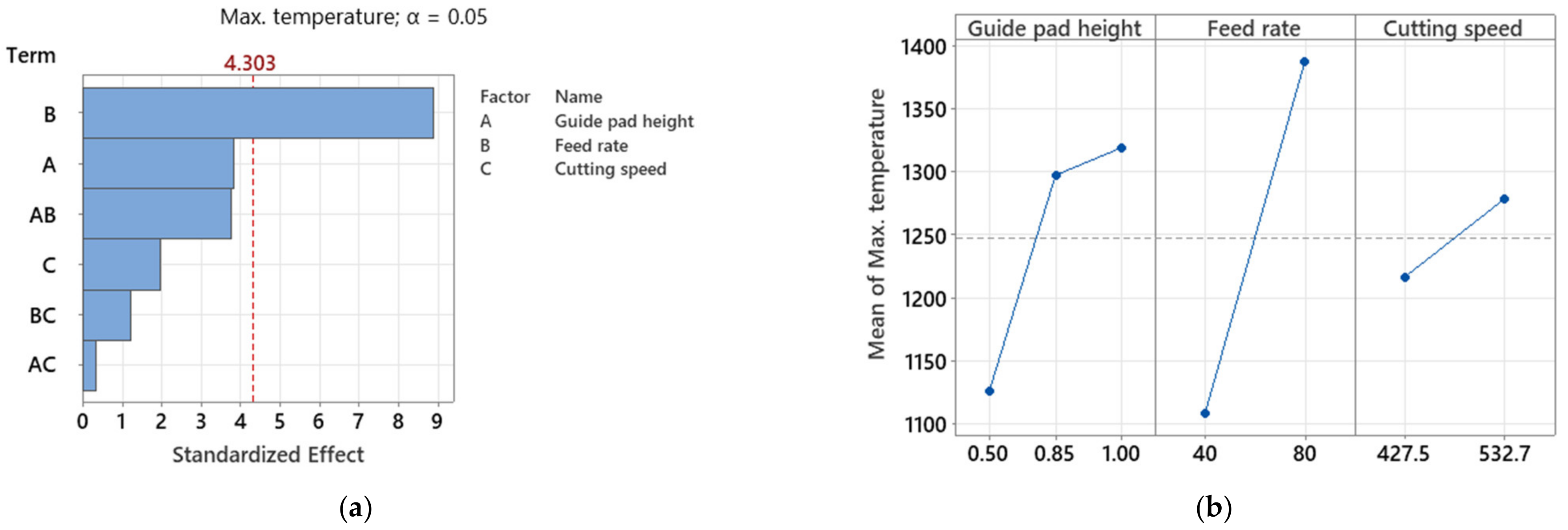
The calculated R2 value, which is a measure for the goodness of a regression, is 98.63%, slightly lower than expected. To visually identify the significant effects, a Pareto chart for standardized effects was created from the calculated values (see Figure 11a).
The Pareto chart plots the absolute values of the standardized effects from the largest effect to the smallest effect. The chart also shows a reference line to indicate which effects are statistically significant. The reference line depends on the significance level α, which is 0.05. Bars that cross the reference line are statistically significant. For the drill head maximum temperature, only the feed rate is above the red line, thus being the only significant factor. Although not all factors are significant, it is important to note how these affect the maximum temperature. Figure 11b shows the main effects plots for the maximum temperature in the drill head. The maximum temperature is directly proportional to all cutting conditions, and the largest effect is on the feed rate. The guide pad height is the second factor with the largest effect; this belongs mainly to the increase from 0.5 to 0.85 mm. By increasing the guide pad height without altering the insert, the contact surface between the guide pads and the workpiece grows, causing increased friction. From 0.85 mm, it is observed how the effect of the height is reduced, and it seems that the temperature approaches a maximum for an increased guide pad height of 1 mm. The cutting speed has the least effect on the maximum temperature on the tool, thus causing the smallest jump.

3.2.2. Feed Force

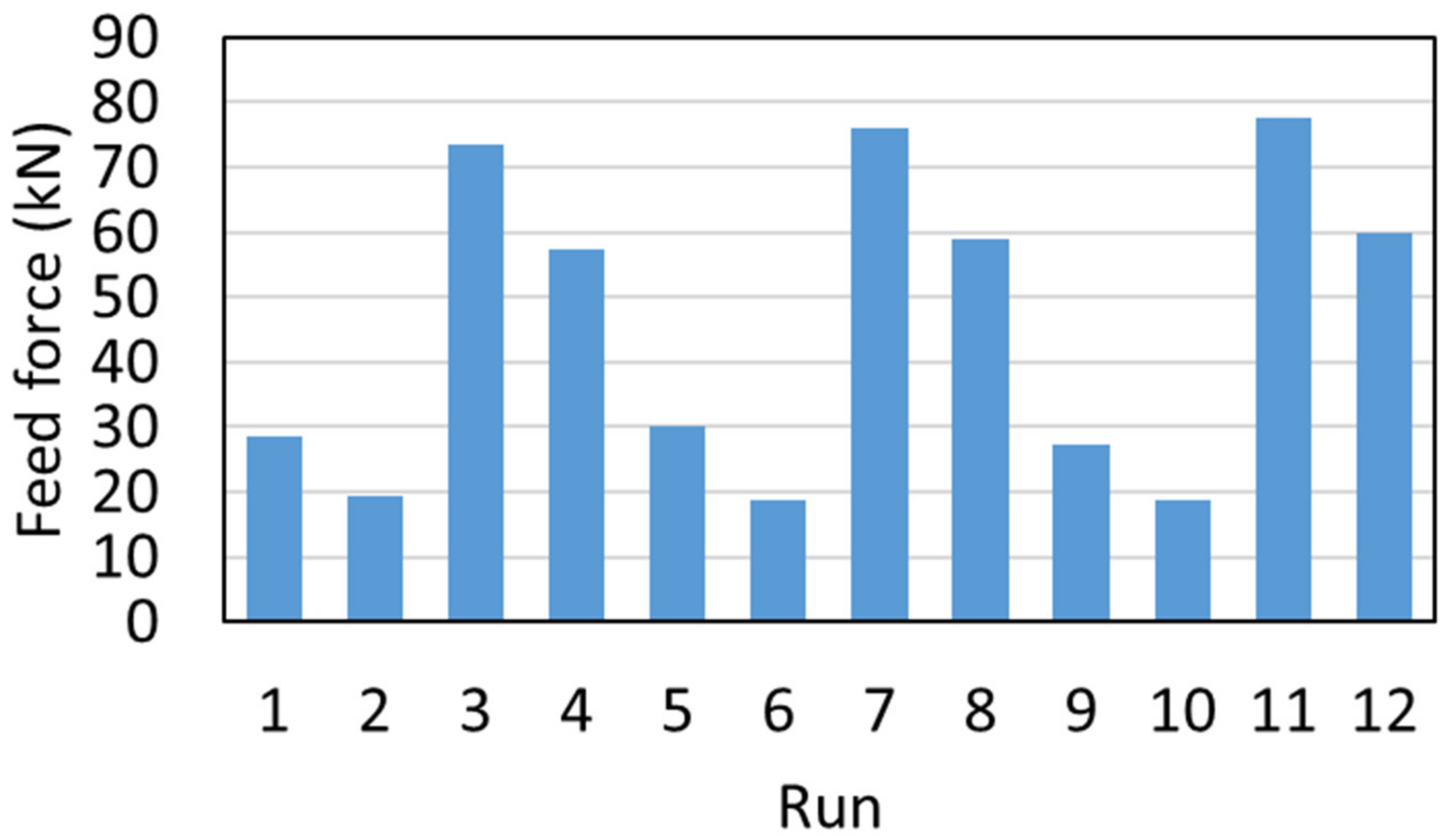
To contrast the results of all cutting conditions, the mean value of the steady-state region is taken into account (see Figure 12).
It can be immediately recognized that the feed force rises with increasing feed rate and decreases with increasing cutting speed. The guide pad height has a low influence on the feed force. To clarify the main effects and significant interactions of the cutting conditions on the feed force, ANOVA was performed. As a result, all the coefficients from the regression model in Equation (4) and the effect of each factor and interaction were obtained (Table 8).
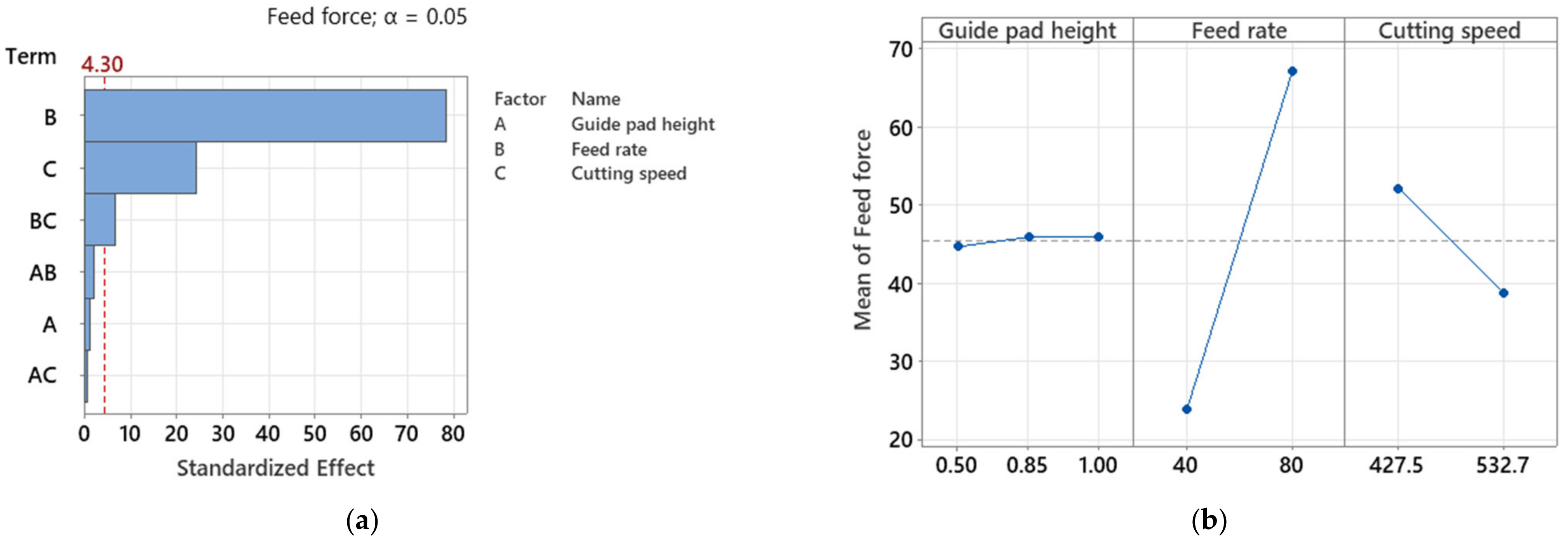
The calculated R2 value of 99.97% indicates a high goodness of the results obtained from the regression model. This is supported by the adjusted coefficient of determination, R2(adj), which is 99.84%. The visualization of the results of this analysis is presented in the Pareto chart in Figure 13a. According to the Pareto chart, the cutting condition with the most significant effect on the feed force is the feed rate, followed by cutting speed and the interaction between them. The main effects plots in Figure 13b demonstrate how the cutting conditions influence the feed force.
The guide pad height forms almost a horizontal line, indicating minimal influence on the feed force. The feed rate shows the largest change in feed force on the main effects plot, the relationship between them being directly proportional. The feed force is inversely proportional to the cutting speed.

3.2.3. Residual Stress

Residual stresses are stresses contained in a solid material despite the absence of external forces. The residual stresses can be either tensile or compressive. Generally, a component contains a combination of both stresses due to the fact that the sum of all residual stresses over the whole component needs to be zero. Residual stresses are formed when a workpiece is subjected to stresses that exceed its elastic limit and plastic deformation occurs. During SLD, non-uniform plastic deformation occurs, inducing the formation of residual stresses.
The residual stresses can be beneficial or detrimental, depending on whether the stress is compressive or tensile. Tensile residual stresses adjacent to the surface can reduce the reliability of components, while compressive residual stresses contribute to the improvement of fatigue strength. For high-performance diesel engines, the basis is an optimized combustion, which is guaranteed by the pulsed injection of fuel under high pressure. For this reason, the use of injection systems capable to endure cyclic compression loads without failure is required. To prevent these systems from failing, the formation of microcracks in component surfaces under high pressures must be avoided. The formation of cracks can be prevented with high surface quality and the targeted introduction of residual stresses in the component subsurface zone. The deep hole of rails (pressure accumulator) is created with SLD. The objective is to produce deep holes with compressive residual stresses on the borehole surface to avoid the formation of microcracks.
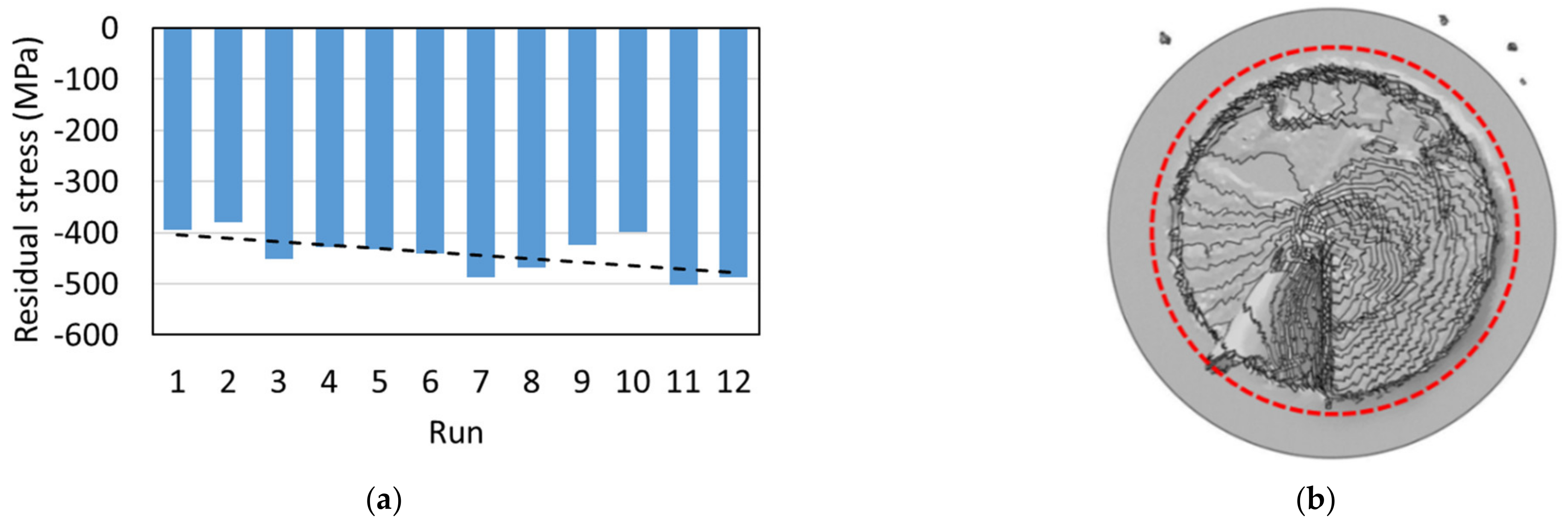
For the determination of the residual stress in the simulations, a subsurface volume was defined (see Figure 14b), which consists of approx. 30,000 elements, obtaining a comparable average stress value for each simulation run. Due to the different orientation of each element with respect to the global coordinate system, the minimal principal stress was evaluated in the subsurface volume. The evaluation of the subsurface in the simulation results delivers average compressive stresses in each simulation run in the range of −379 MPa (run #2) and −502 MPa (run #11). Figure 14a shows the resulting average residual stresses. A clear correlation is observed between increasing guide pad heights and increasing compressive residual stresses, which is indicated by the linear regression line (dashed line). Comparable to the observations for the temperature on the cutting edge (see Figure 11a) but inversely, the values of the runs with an odd number are higher than the residual stress values of the runs with an even number. This means constant parameters, such as the feed rate and the guide pad height, but an increasing cutting speed leads to decreasing compressive stresses. In addition, increasing feed results leads to increasing compressive stresses.
The simulation results are similar to the experimental results (see Figure 9b). The absolute values in the subsurface are comparable to the simulation results.
The influence of the factors on the residual stress in the subsurface were investigated by means of analysis of variance (ANOVA) for the main effects and interactions. As a result, all the coefficients from the regression model in Equation (4) and the effect of each factor and interaction were obtained (Table 9).
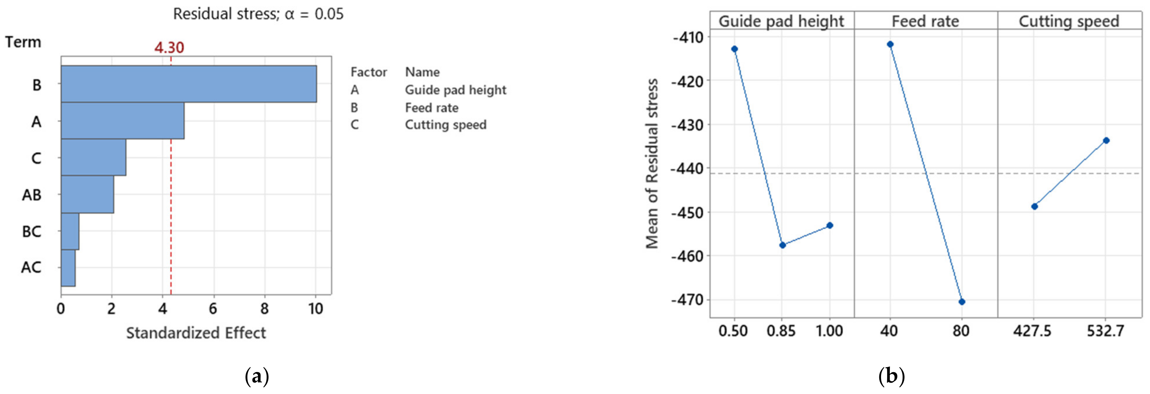
Here, the calculated R2 value of 98.81% indicates a slightly lower goodness of the results obtained from the regression model, which is in the range of the results from the maximum temperature. For visualizing the standardized effects, a Pareto chart for standardized effects was created from the calculated values (see Figure 15a). A significant effect of the feed rate as well as the guide pad heights was observed. This was already indicated by the dashed line in Figure 14a of the model responses. The main effect plot in Figure 15b shows the tendency of the factors. An increasing feed rate leads to increasing compressive stresses. This could be explained by the increasing temperature in the process, which reduces the strength of the material. Thus, the drill head causes higher plastic deformation and finally higher compressive stress. The effect of increasing compressive stress with increasing guide pad height is clear from 0.5 to 0.85 mm but counterintuitive from 0.85 to 1.0 mm, where the compressive stress decreases. The reason for this observation could be the damage model, which eliminates distorted elements from the mesh. Due to the extension of the guide pad to 1.0 mm, more elements with high compressive stresses could be removed. The remaining elements lead to a lower averaged compressive stress value. The influence of the damage model on the residual stress state in the subsurface has to be evaluated in further studies.

4. Conclusions

In this study, a full 3D FE model of an SLD drill head to simulate the drilling process was presented. Based on the results obtained in this study for the DoE analysis, the following conclusions can be drawn:
  • Although some assumptions and simplifications regarding the drill head and the drilling conditions were made, the chip formation and the temperature evolution were reproduced successfully. Moreover, the feeding force evolution as well as the residual stress were modeled with qualitative agreement.
  • A full factorial DoE study was carried out applying three factors with two (feed rate, cutting speed) and three (guide pad height) levels, respectively.
  • The extensive DoE study delivered clear effects of the selected factors, such as the feed rate, cutting speed, and guide pad height, on the maximum temperature in the drill head, the feed force, as well as the residual stress in the subsurface.
  • The regression model delivers an R2 value of 99.97% for the feed force response, which indicates a high goodness of the results. For the responses of the maximum temperature and residual stress, R2 values of 98.63% and 98.81% were obtained, respectively. These values could be improved by more data or another regression model.
  • ANOVA of the maximum temperature shows a significant effect from the feed rate. An increasing feed rate leads to increasing temperatures.
  • Significant effects of the feed rate, cutting speed, and the interaction between both on the feed force were obtained by ANOVA. An increasing feed rate and a decreasing cutting speed lead to larger chips, which have to be cut by the driller. Thus, higher forces occur in the process.
  • The residual stress is significantly affected by the guide pad height and the feed rate. Increasing factors lead to increasing compressive stresses.
  • Regression models for the feed force, maximum temperature, and residual stress were developed, and their corresponding coefficients were successfully determined.
Efforts need to be made to reduce the gap between experiments and simulations, such as performing simulations with lower feed rates or experiments with higher feed rates. This could lead to more accurate validation of the simulations.

Author Contributions

Conceptualization, V.G., R.W., H.-C.M. and S.S.; methodology, V.G. and R.W.; validation, R.W.; formal analysis, D.F.; investigation, D.F., V.G. and R.W.; data curation, R.W.; writing—original draft preparation, D.F. and V.G.; writing—review and editing, H.-C.M. and S.S.; visualization, D.F. and V.G.; supervision, H.-C.M. and S.S.; funding acquisition, H.-C.M. and S.S. All authors have read and agreed to the published version of the manuscript.

Funding

This research was funded by the DFG, grant number SCHM 746/211-1 and MO 2091/6-1. The publication was financially supported by the open access publication fund of the University of Stuttgart.

Data Availability Statement

The data presented in this study are available on request from the corresponding author. The data are not publicly available due to the large amount of data from commercially available simulation and statistical analysis software.

Acknowledgments

The scientific work has been supported by the DFG within the research priority program SPP 2086. The authors thank the DFG for this funding and intensive technical support.

Conflicts of Interest

The authors declare no conflict of interest.

Nomenclature

SLDSingle-lip drill
BTABoring and Trepanning Association
EETElement elimination technique
DoEDesign of experiment
CADComputer-aided design
PTCPositive temperature coefficient
FEMFinite element method
JCJohnson–Cook
ANOVAAnalysis of variance
fFeed per tooth, mm/rev
vcCutting speed, m/min
ρDensity, kg/m3
νPoisson’s ratio
EYoung’s modulus, GPa
εStrain, mm/mm
σFlow stress, MPa
ε ˙ Strain rate, 1/s
λStress triaxiality
hGPGuide pad height, mm
δConductivity, W/m K
αThermal expansion coefficient, µm/m K
kGap conductance, W/m2 K
qHeat flux per unit area, W/m2
TTemperature, K
TaAmbient temperature, K
TmMelting temperature, K

References

  1. Kumari, P. Drilling Machine Market. Available online: alliedmarketresearch.com (accessed on 31 March 2021).
  2. Biermann, D.; Bleicher, F.; Heisel, U.; Klocke, F.; Möhring, H.C.; Shih, A. Deep hole drilling. CIRP Ann. 2018, 67, 673–694. [Google Scholar] [CrossRef]
  3. Biermann, D.; Heilmann, M.; Kirschner, M. Analysis of the Influence of Tool Geometry on Surface Integrity in Single-lip Deep Hole Drillingwith Small Diameters. Procedia Eng. 2011, 19, 16–21. [Google Scholar] [CrossRef] [Green Version]
  4. Agmell, M.; Ahadi, A.; Ståhl, J. A fully coupled thermomechanical two-dimensional simulation model for orthogonal cutting: Formulation and simulation. Proc. Inst. Mech. Eng. B 2011, 225, 1735–1745. [Google Scholar] [CrossRef]
  5. Agmell, M.; Ahadi, A.; Gutnichenko, O.; Ståhl, J. The influence of tool micro-geometry on stress distribution in turning operations of AISI 4140 by FE analysis. Int. J. Adv. Manuf. Technol. 2017, 89, 9–12. [Google Scholar] [CrossRef] [Green Version]
  6. Persson, H.; Agmell, M.; Bushlya, V.; Ståhl, J. Experimental and numerical investigation of burr formation in intermittent turning of AISI 4140. Procedia CIRP 2017, 58, 37–42. [Google Scholar] [CrossRef]
  7. Arrazola, P.J.; Özel, T.; Umbrello, D.; Davies, M.; Jawahir, I.S. Recent advances in modelling of metal machining processes. CIRP Ann. 2013, 62, 695–718. [Google Scholar] [CrossRef]
  8. Pimenov, D.Y.; Guzeev, V.I. Mathematical model of plowing forces to account for flank wear using FEM modeling for orthogonal cutting scheme. Int. J. Adv. Manuf. Technol. 2017, 89, 3149–3159. [Google Scholar] [CrossRef]
  9. Pantalé, O.; Bacaria, J.L.; Dalverny, O.; Rakotomalala, R.; Caperaa, S. 2D and 3D numerical models of metal cutting with damage effects. Comput. Methods Appl. Mech. Eng. 2004, 193, 4383–4399. [Google Scholar] [CrossRef] [Green Version]
  10. Wegert, R.; Guski, V.; Schmauder, S.; Möhring, H.C. Effects on surface and peripheral zone during single lip deep hole drilling. Procedia Cirp 2020, 87, 113–118. [Google Scholar] [CrossRef]
  11. Aveiro, P. Design of Experiments in Production Engineering; Davim, J.P., Ed.; Springer International Publishing: Basel, Switzerland, 2016. [Google Scholar]
  12. Kyratsis, P.; Bilalis, N.; Antoniadis, A. CAD-based simulations and design of experiments for determining thrust force in drilling operations. Comput. Aided Des. 2011, 43, 1879–1890. [Google Scholar] [CrossRef]
  13. Chatterjee, S.; Mahapatra, S.S.; Abhishek, K. Simulation and optimization of machining parameters in drilling of titanium alloys. Simul. Model. Pr. Theory 2016, 62, 31–48. [Google Scholar] [CrossRef]
  14. Wegert, R.; Guski, V.; Möhring, H.C.; Schmauder, S. Determination of thermo-mechanical quantities with a sensor-integrated tool for single lip deep hole drilling. Procedia Manuf. 2020, 52, 73–78. [Google Scholar] [CrossRef]
  15. Wegert, R.; Guski, V.; Möhring, H.C.; Schmauder, S. Temperature monitoring in the subsurface during single lip deep hole drilling: Measuring of the thermo-mechanical load at different cutting parameters, including wear and simulative validation. tm-Tech. Mess. 2020, 87, 757–767. [Google Scholar] [CrossRef]
  16. Brnic, J.; Turkalj, G.; Canadija, M.; Lanc, D.; Brcic, M. Study of the effects of high temperatures on the engineering properties of steel 42CrMo4. High Temp. Mater. Process. 2015, 34, 27–34. [Google Scholar] [CrossRef]
  17. Storchak, M.; Rupp, P.; Möhring, H.C.; Stehle, T. Determination of Johnson–Cook constitutive parameters for cutting simulations. Metals 2019, 9, 473. [Google Scholar] [CrossRef] [Green Version]
  18. Johnson, G.R.; Cook, W.H. Fracture characteristics of three metals subjected to various strains, strain rates, temperatures and pressures. Eng. Fract. Mech. 1985, 21, 31–48. [Google Scholar] [CrossRef]
  19. ABAQUS. Version 2018, ABAQUS Documentation, Dessault Systems Simulia Corp; ABAQUS: Providence, RI, USA, 2018. [Google Scholar]
  20. Barge, M.; Hamdi, H.; Rech, J.; Bergheau, J. Numerical modelling of orthogonal cutting: Influence of numerical parameters. J. Mater. Process. Technol. 2005, 164, 1148–1153. [Google Scholar] [CrossRef]
  21. Mabrouki, T.; Rigal, J. A contribution to a qualitative understanding of thermo-mechanical effects during chip formation in hard turning. J. Mater. Process. Technol. 2006, 176, 214–221. [Google Scholar] [CrossRef]
  22. Schulze, V.; Michna, J.; Zanger, F.; Faltin, C.; Maas, U.; Schneider, J. Influence of cutting parameters, tool coatings and friction on the process heat in cutting processes and phase transformations in workpiece surface layers. Htm J. Heat Treat. Mater. 2013, 68, 22–31. [Google Scholar] [CrossRef]
  23. Fluhrer, J. DEFORM 3D Version 6.1 User´s Manual; Scientific Forming Technologies Corporation-SFTC: Columbus, OH, USA, 2007. [Google Scholar]
  24. Koric, S.; Hibbeler, L.; Thomas, B. Explicit coupled thermo-mechanical finite element model of steel solidification. Int. J. Numer. Methods Eng. 2009, 78, 1–31. [Google Scholar] [CrossRef] [Green Version]
  25. Prior, M. Applications of implicit and explicit finite element techniques to metal forming. J. Mater. Process. Technol. 1994, 45, 649–656. [Google Scholar] [CrossRef]
  26. Rajput, R. A Textbook of Manufacturing Technology: Manufacturing Processes; Laxmi Publications: New Delhi, India, 2007. [Google Scholar]
  27. ASTM. E837: Standard Test Method for Determining Residual Stresses by the Hole-Drilling Strain-Gage Method; ASTM International: West Conshohocken, PA, USA, 2013. [Google Scholar]
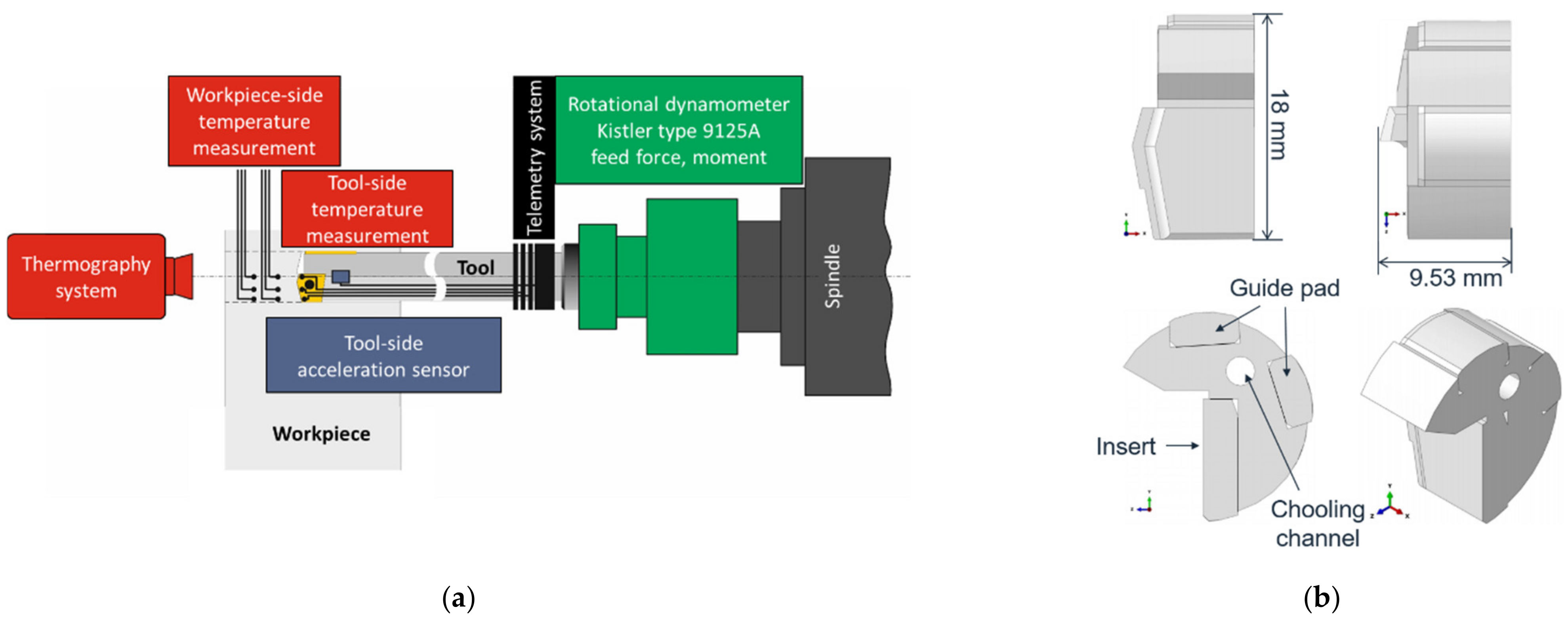
Figure 1. Schematic representation of the experimental setup for SLD (a) and CAD of the single-lip deep drill with a changeable insert and guiding pads from the company Gühring AG for the FEM simulation (b).
Jmmp 05 00044 g001
Figure 2. Feed force evolution (a) and drilling torque evolution (b) measured in an experiment for a cutting depth of 20 mm, a feed of 0.042 mm/rev, and a cutting speed of 68 m/min [10].
Jmmp 05 00044 g002
Figure 3. Thermography image of the backside of the workpiece at the moment of breakthrough (a) and maximum temperature at the cutting edge measured in the experiment (b) [10].
Jmmp 05 00044 g003
Figure 4. Location of the reference point (a) and symmetry/antisymmety/encastre boundary condition (b).
Jmmp 05 00044 g004
Figure 5. Discretization of the drill head (a) and of the workpiece (b).
Jmmp 05 00044 g005
Figure 6. Definition of guide pad height (a) and chip formation after 0.055 s with a feed of 0.64 mm/rev (80 mm/s) and a cutting speed of 427.5 m/min (b).
Jmmp 05 00044 g006
Figure 7. Lateral and front views of the formed chip with a feed of 0.64 mm/rev and a cutting speed of 427.5 m/min in the simulation (a) and chips obtained from the experiment (b).
Jmmp 05 00044 g007
Figure 8. Temperature in the drill head under the following cutting conditions: a feed of 0.64 mm/rev and a cutting speed of 472.5 m/min (a). Development of the maximum temperature at the cutting edge and the drill head with a feed of 0.64 mm/rev and a cutting speed of 472.5 m/min in the simulation (b).
Jmmp 05 00044 g008
Figure 9. Simulated feed force evolution applying a feed of 0.64 mm/rev and a cutting speed of 472.5 m/min (a) and tangential residual stresses after one rotation with a feed of 0.64 mm/rev and a cutting speed of 472.5 m/min (b).
Jmmp 05 00044 g009
Figure 10. Average temperature at the cutting edge in the steady-state region (a) and maximum temperature in the drill head (b).
Jmmp 05 00044 g010
Figure 11. Pareto chart of the standardized effects for drill head maximum temperature (a) and main effects plot for drill head maximum temperature (b).
Jmmp 05 00044 g011
Figure 12. Average feed force in the steady-state region.
Jmmp 05 00044 g012
Figure 13. Pareto chart of the standardized effects for the feed force (a) and main effects plot for the feed force (b).
Jmmp 05 00044 g013
Figure 14. Influence of the cutting conditions on the average residual stress (a) and representation of the evaluated subsurface volume (b).
Jmmp 05 00044 g014
Figure 15. Pareto chart of the standardized effects for the residual stress (a) and main effects plot for the residual stress (b).
Jmmp 05 00044 g015
Table 1. Elastic properties of DIN 42CrMo4 [16].
Young’s Modulus (GPa)Poisson’s Ratio (-)Temperature (K)
2170.3173
2130.3273
2120.3293
2070.3373
1990.3473
1920.3573
1840.3673
1750.3773
1640.3873
690.31773
Table 2. Input data for the Johnson–Cook constitutive equation to model the plasticity behavior of DIN 42CrMo4 based on [9,16].
A
(MPa)
B
(MPa)
C
(-)
n
(-)
m
(-)
Tm
(K)
Ta
(K)
5955800.0230.1331.031793300
Table 3. Input data for the Johnson–Cook damage initiation model.
d1d2d3d4d5 T m
(K)
T a
(K)
ε ˙ 0
(1/s)
0.10.04−0.0210.1217933001
Table 4. Thermal expansion, conductivity, and specific heat of DIN 42CrMo4, depending on the temperature [22].
Temperature (K)Thermal Expansion (µm/m K)Conductivity (W/m K)Specific Heat (J/kg K)
17310.8-291.24
27311.7-354.04
29311.941.7361.89
37312.543.4389.36
47313.043.2418.41
57313.641.4445.88
67314.139.1479.64
77314.536.7531.45
87314.934.1610.73
177314.934.1610.73
1923-34.1610.73
Table 5. Input data for the tool material made of tungsten carbide with 15% cobalt [23].
PropertyUnitValue
Density, ρkg/m315,700
Young’s modulus, EGPa524
Poisson’s ratio, ν-0.23
Thermal expansion, αµm/m K6.3
Conductivity, δW/m K82.2404
Specific heat, CpJ/kg K579.45
Table 6. Full factorial experiment.
Run OrderGuide Pad Height (mm)Feed Rate (mm/s)Cutting Speed (m/min)
10.540427.5
20.540532.7
30.580427.5
40.580532.7
50.8540427.5
60.8540532.7
70.8580427.5
80.8580532.7
91.0040427.5
101.0040532.7
111.0080427.5
121.0080532.7
Table 7. Estimated effects and coefficients for the maximum temperature in the drill head.
TermCoefficientSE CoefficientT-Valuep-Value
Constant1247.715.879.050.0
Guide pad height (A)
0.5−121.722.3−5.450.032
0.8549.822.32.230.155
Feed rate (B)
40−140.015.8−8.870.012
Cutting speed (C)
427.5−31.215.8−1.970.187
Guide pad height, feed rate (AB)
0.50, 40121.022.35.420.032
0.85, 40−59.022.3−2.640.118
Guide pad height, Cutting speed (AC)
0.50, 427.5−17.322.3−0.780.519
0.85, 427.512.722.30.570.628
Feed rate, cutting speed (BC)
40, 427.5−19.515.8−1.240.342
S = 54.6717; R2 = 98.63%; R2(adj) = 92.48%.
Table 8. Estimated effects and coefficients for the feed force.
TermCoefficientSE CoefficientT-Valuep-Value
Constant45.4460.277164.190.0
Guide pad height (A)
0.5−0.8130.391−2.080.172
0.850.4040.3911.030.410
Feed rate (B)
40−21.6720.277−78.300.0
Cutting speed (C)
427.56.6830.27724.140.002
Guide pad height, feed rate (AB)
0.50, 400.9700.3912.480.131
0.85, 400.2070.3910.530.649
Guide pad height, cutting speed (AC)
0.50, 427.5−0.3850.391−0.980.429
0.85, 427.50.4270.3911.090.389
Feed rate, cutting speed (BC)
40, 427.5−1.8620.277−6.730.021
S = 0.958840; R2 = 99.97%; R2(adj) = 99.84%.
Table 9. Estimated effects and coefficients for the residual stress.
TermCoefficientSE CoefficientT-Valuep-Value
Constant441.152.94−150.240.0
Guide pad height (A)
0.5028.464.156.850.021
0.85−16.454.15−3.960.058
Feed rate (B)
4029.402.9410.010.010
Cutting speed (C)
427.5−7.512.94−2.560.125
Guide pad height, feed rate (AB)
0.50, 40−3.214.15−0.770.520
0.85, 40−9.204.15−2.220.157
Guide pad height, cutting speed (AC)
0.50, 427.5−2.254.15−0.540.642
0.85, 427.54.594.151.100.384
Feed rate, cutting speed (BC)
40, 427.52.102.940.720.549
S = 10.1713; R2 = 98.81%; R2(adj) = 93.43%.
Publisher’s Note: MDPI stays neutral with regard to jurisdictional claims in published maps and institutional affiliations.