Abstract
Multiturn coils are required for manufacturing sheet metal parts with varying depths and special geometrical features using electromagnetic forming (EMF). Due to close coil turns, the physical phenomena of the proximity effect and Lorentz forces between the parallel coil windings are observed. This work attempts to investigate the mechanical consequences of these phenomena using numerical and experimental methods. A numerical model was developed in LS-DYNA. It was validated using experimental post-mortem strain and laser-based velocity measurements after and during the experiments, respectively. It was observed that the proximity effect in the parallel conductors led to current density localization at the closest or furthest ends of the conductor cross-section and high local curvature of the formed sheet. Further analysis of the forces between two coil windings explained the departure from the “inverse-distance” rule observed in the literature. Finally, some measures to prevent or reduce undesired coil deformation are provided.
1. Introduction
Electromagnetic forming (EMF) is a noncontact forming process involving the deformation of sheets with high electrical conductivity by the discharge of pulsed electrical power. This process comes under the broad umbrella of impulse-based or high-speed forming processes, as strain rates obtained during the process range from 103 to 104 s−1. Psyk et al. [1] describe the process of electromagnetic forming as obtaining a pulsed current by discharging a capacitor bank (or many). This current is time-varying and damped sinusoidal in nature. With the time-varying magnetic field, which accompanies the current and is concentrated between the coil and the workpiece, eddy currents are induced in the workpiece. Psyk et al. [1] also mention the presence of Maxwell pressure, a magnetic pressure that acts on the workpiece and deforms it by exceeding flow stress. Workpiece velocities of several hundred meters per second have been reported by Ahmed et al. [2] and Demir et al. [3] with Thibaudeau et al. [4] observing velocities between 100 and 300 m/s. The setup for electromagnetic forming is shown in Figure 1. The figure shows a general coil geometry forming a general sheet geometry, with setups to measure the current and workpiece velocity.
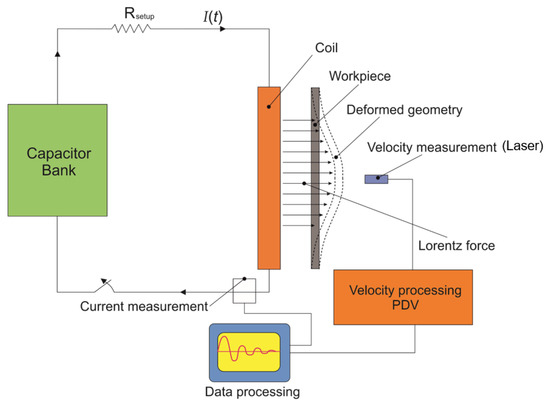
Figure 1.
General experimental and measurement setup for electromagnetic forming.
The process offers many advantages over conventional sheet metal forming processes, such as higher forming limits reported by Demir et al. [3], reduction of springback reported by Gayakwad et al. [5], possibility to perform operations, such as coining and embossing reported by Psyk et al. [1].
1.1. Context of the Research
Extensive research has been devoted to applying the principles of electromagnetic induction to achieve compression or expansion of tubes and rings, welding of tubes and sheets, as well as cutting of sheets. In addition, the performance of the process has been improved by the design of coils, capacitor banks with shorter discharge times, and higher charging energies and high-speed measurements. Numerical modeling of the process, e.g., as introduced by Takatsu et al. [6] for a flat spiral coil, also helps visualize the process and observe the development of various unmeasurable parameters during the process.
With the understanding of the process dynamics established, the focus turned to the comprehensive study of process parameters, such as characteristics of the pulsed current, coil geometry, and tool life of the coil. Coils have been examined for their mechanical and thermal aspects, such as in the study by Gies et al. [7], in which the temperature distribution of the coil was identified to determine conclusions about the long-term usage of the coil.
This work examines another important parameter, namely, the distance between potentially multiple windings of coils. This is also known as the proximity of the coils.
1.2. Tool Life and Geometries of Electromagnetic Forming Coils
As EMF is a noncontact process, the role of the tool is taken by the coil (like a punch in deep drawing). As one of the most important parts of the setup, Golovaschenko [8] recommends that the objective for coil optimization should be the improvement in the ability to withstand many repeated discharges. Taebi et al. [9] propose that the optimization approach adjust the coils’ geometrical parameters based on the deviation of the obtained workpiece geometry from the required geometry, which serves as an objective function. Thibaudeau et al. [4] state that for a given part, the coil design process should involve the decision of whether a high-pressure or a high velocity is needed. If the requirement is to have high magnetic pressure, a coil with a high number of turns must be selected, while for the latter case, a coil with a smaller number of turns must be selected, as this would lead to a shorter rise to the peak current. Coils used for processes, such as embossing and forming into shallow features, require multiturn coils with a high number of turns, as reported by Watanabe and Kumai [10]. The use of many turns for applications with small and restricted geometries of the workpiece leads to reduced spacing and dimensions of the coil.
1.3. Skin and Proximity Effects between Conductors
The skin effect can be defined as the concentration of the current in the outer annulus of the conductor at high frequencies. It has been observed in many analyses, e.g., by Dwight [11] and Kennelly [12]. Due to this so-called crowding of the current at the outer periphery of the conductor, the alternating current (AC) resistance of the conductor is much higher than its direct current (DC) resistance, according to Reatti et al. [13]. This leads to increased power loss. Sigg et al. [14] emphasize that even though the calculation of eddy current effects and the AC resistance is essential, analytical methods for doing so are limited to simple geometries, as it is required to solve Maxwell’s equations in inhomogeneous unbounded regions. Popovic [15] states that the skin depth δ can be obtained using Equation (1), where is the angular frequency, is the permittivity of the material and is the electrical conductivity:
The skin effect is due to the generation of eddy currents induced by the magnetic field of the primary current. In the center of the conductor, this eddy current cancels the primary current but reinforces the current flow at the periphery, according to Riba [16].
When dealing with multiple conductors or windings of the same conductor, the proximity effect comes into play because the current density of the conductors is affected by the current flowing in the neighboring conductors. This form of inductive coupling is known as the proximity effect, which becomes more pronounced at higher frequencies and small spacings between the conductors. Depending on the direction of the current flow, the proximity effect increases the current density at certain locations and reduces the same at other locations. If the current in adjacent coils is flowing in the same direction, then the current density is the highest in the furthest corners of the coils and vice versa.
Riba [16] states that the mathematical analysis of the proximity effect is even more difficult than that of the skin effect and possible only for a very few geometries. An analytical determination of the skin and proximity effects separately is attempted by Abdelbagi [17]. For two parallel plates with rectangular cross-sections, Abdelbagi [17] considers the flow of current in two plates in the same and opposite directions by solving the corresponding Helmholtz equation.
While this development is helpful in the analysis of the proximity effect in conductors with rectangular cross-sections, the underlying assumption of the nullification of the current density at the near conductor end ignores the actual effect of the spacing between the conductors. Furthermore, in electromagnetic forming, the additional presence of a conducting workpiece also modifies the current density distribution. The model to include the combined proximity effect due to the workpiece, the other coil windings, and the inherent skin effect at typical frequencies is predicted to be mathematically very complex and hardly scalable to many coils turns or complex coil geometries. Such a conclusion leads to using numerical models rather than analytical ones for solving complex electromagnetic problems. Vitelli [18] attempted to evaluate the current density and the subsequent losses in two conductors due to the proximity effect numerically.
1.4. Purpose of the Study
The objective of the present article is to evaluate the effect of spacing (proximity) between coil windings and its effect on their deformation and the forming of the workpiece in EMF. The primary objective above can be divided into three secondary objectives as follows:
- To develop and experimentally verify a numerical model to investigate the forming of the workpiece for various coil proximities and input energies;
- To evaluate the coil deformation for various discharge energies, cross-sections, and numbers of coils, so that this can be avoided in prospective applications.
2. Materials and Methods
2.1. Numerical Modeling in LS-DYNA
2.1.1. Development of the Simulation
As the EMF process is completed in a very small amount of time (approximately 200 µs), a transient numerical model provides a deeper understanding of the process evolution. The numerical model was developed employing the finite element code LS-DYNA, which provides the possibility to model the electromagnetic aspects of the problem along with the thermal and mechanical aspects in a coupled method. The methodology and theory of numerical modeling of electromagnetic forming are established by L’ Éplattenier [19], with the same approach being implemented here. There, the surrounding air is modeled using the boundary element method (BEM). In this way, the air does not need to be meshed, and higher deformations of the parts are possible without continuous re-adaptation of the air mesh. The numerical model can provide information about the various parameters that cannot be measured directly, such as current densities, Lorentz forces, and the magnetic field. The simulation arrangement is presented in Figure 2.
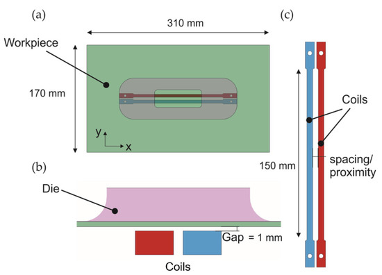
Figure 2.
Numerical model in LS-DYNA. (a) Top view showing the dimensions of the workpiece; (b) front view showing the relative arrangement of the setup, (c) arrangement of the coils relative to one another for various values of spacing.
The arrangement consists of two (or more) identical coils, which are connected in parallel. To ensure that the coils are connected in parallel, the total input current is divided by the number of coils. This input current is obtained from the experiments, as described in Section 2.3.3. A sample input current provided to the simulation is presented in Figure 3. This current is damped sinusoidal with a reducing frequency.
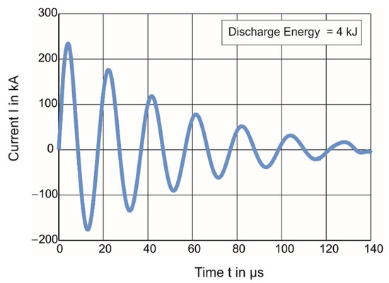
Figure 3.
Input current curve for the simulations obtained for a discharge energy E0 of 4 kJ. This current is distributed in both coils.
The material assigned to both the coils is copper alloy CuCr1Zr, which compared to wrought pure copper alloy, has lower electrical conductivity, yet excellent mechanical strength. The holes at the ends of both the coils are fixed by constraining all displacements and rotations. The workpiece is modeled to be aluminum alloy EN AW-5083-H111, with a thickness of 1 mm. The other dimensions of the workpiece were chosen according to the requirements of the experimental setup. The gap between the workpiece and the coils was set to 1 mm. The workpiece and the coils were both modeled as deformable elastic-plastic solids. The die used for the open-window electromagnetic forming process was modeled as a rigid, nonconducting and fixed shell.
In coils with a workpiece above them, the current flows close to the coil’s top surface. The coil induces a current in the opposite direction in the workpiece, and the currents flow as close as possible to one another due to the proximity effect, as explained in Section 1.3. This effect was also observed and modeled by Gies [20]. Similar straight coils were meshed so that the mesh density closer to the workpiece was high (thinner elements) and reduced gradually towards the opposite direction. This is done to capture the higher surface current density more precisely with a higher number of nodes in the vicinity. However, due to the very thin elements at the top, the aspect ratio of the elements is greatly skewed. In large deformations, such elements are prone to nonconvergence, erroneous results and long solving times. The mesh used for the coils is shown in Figure 4. The thickness of the topmost element is comparable to the calculated skin depth but experiences a high variation of current density within itself. Attempts with smaller thicknesses led to nonconvergence of the electromagnetic solver in LS-DYNA. The workpiece was meshed with two elements along the thickness, capturing the skin depth calculated at a frequency of 58,000 Hz (average obtained from various measurements), of EN AW-5083 sufficiently. Liu [21] stated that the deformation of the workpiece continues after the discharge of the current is finished. This happens due to the inertia of the workpiece. Furthermore, Gies [20] observed and modeled the temperature distribution in the numerical model until much longer after the process completion. The simulations were run for 0.009 s, when the deformation of the workpiece was observed to be completely stabilized for 90% of the run of the simulation.
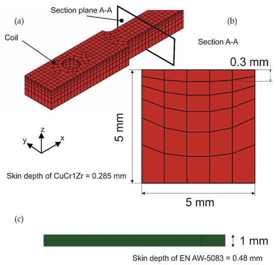
Figure 4.
Meshing of the coil for the numerical model. (a) View of the coil end and the hole feature; (b) cross-sectional view showing thinner top element layers (c) cross-sectional view showing thickness-elements of the workpiece.
2.1.2. Material Models and Data
The properties assigned to the components can be classified into electrical, thermal and mechanical properties. The electrical conductivity (), thermal conductivity () and heat capacity () vs. temperature for CuCr1Zr and EN AW-5083 is shown in Table 1.

Table 1.
Electrical and thermal properties for CuCr1Zr and EN AW-5083.
For EN AW-5083, the electrical conductivity is provided only at a room temperature of 19 MS/m. For CuCr1Zr, the plastic properties are provided as dependent on temperature. These properties were determined by hot tensile tests and were extrapolated exponentially, shown in Figure 5. The strain-rate dependency of CuCr1Zr was ignored.
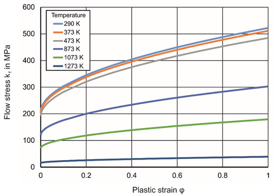
Figure 5.
Temperature-dependent stress-plastic strain flow properties of CuCr1Zr from high-temperature tensile tests and extrapolation exponentially.
The Young’s modulus of EN AW-5083 was taken as 70 Gpa; the Poisson’s ratio was taken as 0.33. The plastic behavior of EN AW-5083 was defined to be both strain-rate- and temperature-dependent. The strain-rate sensitivity of plastic flow of aluminum alloys is assumed low until 103 s−1, but a sharp rise is observed at strain rates between 103 s−1 and 104 s−1. For few aluminum alloys, this dependence of initial flow stress on the strain rate is shown by Weddeling et al. [22]. Clausen et al. [23] observed that for AA-5083-H116 (different temper than the currently used alloy), the material shows negative strain-rate sensitivity for low strains (softening when the strain rate is increased). For higher strain rates (more than 1 s−1), the strain-rate sensitivity is positive. Until 103 s−1, the material data for aluminum is based on high-temperature and high strain-rate tensile tests. For strain rates higher than 104 s−1, the flow curves are not readily available or easily measured. The sudden change in the initial flow stress for aluminum alloys is attributed to a change in deformation mechanism, according to Kabirian [24]. The mechanism for deformation at very high strain rates is the viscous drag of the dislocations. A mechanism-based constitutive relation is suggested, which is shown in Equation (2). In this equation, is the flow stress at a given strain rate and temperature, is the flow stress at a strain rate of 1 s−1, is the melting temperature, presents the sigmoidal feature of the function and is the strain rate:
For the current case, the exponential relation proposed for very high strain rates is relevant. This relation was used to predict the flow stresses for strain rates of 104 s−1 and above, with as the flow stress for lower strain rates (any lower strain rate can be chosen as the sensitivity at lower strain rates is very small). The final flow curves used in the simulations (at room temperature) are shown in Figure 6. The flow curves for strain rates of 0.001 s−1 and 1000 s−1 are almost identical due to the negligible strain-rate sensitivity of the material in this regime. As the flow curves for all strain rates in this regime are almost identical, they have not been provided in Figure 6.
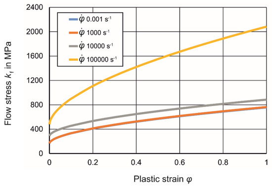
Figure 6.
Implementation of the model proposed by Kabirian [24] to determine strain-rate-dependent flow curves for EN AW-5083, represents the strain rate in 1/s.
In LS-DYNA, the flow curves (experimentally measured and extrapolated both) are provided to the solver in the form of tabular data. The material model used in LS-DYNA is denoted as MAT_106, which is an elastic-viscoplastic-thermal model. The strain dependence is expressed in terms of the sum of exponential terms, and the strain-rate dependence is expressed using the Cowper–Symonds model. From the provided tabular data, the parameters of the material model are calculated by the solver.
2.2. Numerical Modeling in FEMM
Development of the Simulation
FEMM is an open-source finite element software for a harmonic 2D or axisymmetric modeling of electromagnetics. The advantage in using FEMM is the ability to quickly model a simplified version of the present problem for efficient further processing (compared to the computationally much more costly LS-DYNA model). The cross-sections of the two coils, along with the cross-section of the sheet, are modeled. The boundary condition of the zero magnetic fields is applied at a large distance away from the coils and the workpiece.
The input of the current in FEMM happens by providing amplitude and a frequency, after which a constant sinusoidal current is applied. As the actual current, as shown in Figure 3, is damped sinusoidal, only the first half-wave of the current is modeled by using the amplitude and frequency of the same. While the number of elements in the cross-section of the coil is only 30 in the LS-DYNA model, the number of cross-section elements in the FEMM model is upwards of 10,000 with only a minor impact of total solving time and no impact on convergence. Only room temperature values for the electrical conductivity for CuCr1Zr and EN AW-5083 are input into FEMM. These values are given in Section 2.1.2.
2.3. Experimental Analysis
2.3.1. Experimental Setup
The experimental setup includes the capacitor bank for the discharge of energy, the coil setup with two or more coils for the study, the EN AW-5083 workpiece and the equipment for clamping and safety. The capacitor bank used for the analysis was the SMU612 by the company Poynting. The main characteristics of this capacitor bank are given in Table 2.
Table 2.
Characteristics of capacitor bank SMU612.
When the bank is discharged, the current flows through the circuit into the coil setup and is suitably distributed into the coils, which are connected in a parallel system. The CAD model of the coil setup used for the experiments is shown in Figure 7. The coils are connected to the setup using M3 screws, which are expected to serve as fixed support. The geometry of the coil used for the experiments is shown in Figure 2. The cross-section of the coil is 5 mm 5 mm, similar to the ones used by Gies [7]. The width of the ends was reduced to ensure closer proximities between the coils.
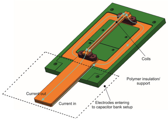
Figure 7.
CAD model of the coil setup used for the experiments. The path of the current is shown in blue. Some support elements have not been shown for clarity of representation.
2.3.2. Parameters Studied in the Experiments
To study the effect of the spacing between the coils, the spacing was varied between 4 mm and 9 mm at an interval of 1 mm. Spacings smaller than 4 mm were not possible due to the geometry of the coil. Therefore, the effect of smaller intervals was investigated through the numerical models. For each value of spacing, various energies ranging from 3 kJ to 6 kJ were discharged, and the deformation of the coil and the workpiece were recorded.
For some experiments, coils of higher cross-sections were used as possibilities to reduce the coil deformation. The cross-sections investigated were 5 mm × 10 mm and 10 mm × 5 mm. The three cross-sections used are shown in Figure 8.
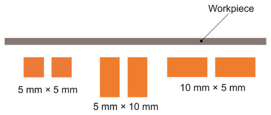
Figure 8.
Three different coil cross-sections studied for the experiments.
2.3.3. Measurement Methods
The parameters measured in the experiments, along with the techniques used to measure them, are described below: The total discharge current was measured using a Rogowski coil with a conversion factor of 1.2 mV/A. Strain measurement was performed after the process is complete. Before the process, a pattern, which is a grid of dots, is created on the top surface of the EN AW-5083 sheet by selective anodizing. After the process, the deformed pattern is analyzed by the optical strain measurement system ARGUS by GOM. The parameter of interest measured through this setup is the von Mises equivalent plastic strain. The ARGUS system can measure only the two surface strains. The thickness strain is estimated using the volume constancy law in plasticity and the assumption that the strain is uniform across the thickness. The displacement of the coils was measured using ATOS by GOM also after the completion of the process. ATOS is an optical coordinate–measuring setup. The displacements were computed by comparing the original and the deformed geometries. As both the strain measurement of the workpiece and the displacement measurement of the coils could only be conducted after the experiments, the vertical velocity of the center of the specimen (middle point) was measured during the process using photonic Doppler velocimetry (PDV), as explained by Moro [25], which is a laser-based system that uses the phase shift in the reflected beam to determine the signal.
3. Results
3.1. Validation of the Numerical Model
The numerical model was verified by comparing the post-experiment strains and the apex velocity during the process.
3.1.1. Comparison of Plastic Strains
The strains measured from the experiments at the end of the process are the plastic strains on the sheet surface. They are compared to the effective plastic strains from LS-DYNA. The comparison was made along specific paths. Path 1 is the path along the coil in the middle of the two coils and the workpiece. The deformation along this path happens mostly due to inertia. Path 2 is the path across the workpiece in the y-direction. These paths are shown in Figure 9. The comparison for the numerically and experimentally determined strains is shown in Figure 10 for path 1.
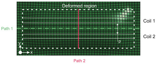
Figure 9.
Two different paths chosen for comparison of plastic strains from the numerical and experimental analyses (top view).
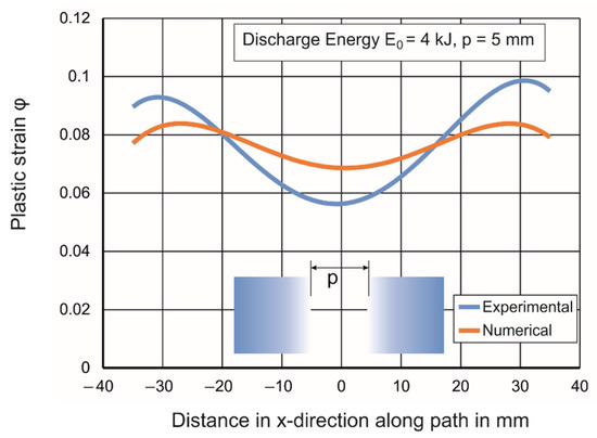
Figure 10.
Comparison of numerical and experimental equivalent plastic strains.
This process was repeated for various discharge energies and spacings between the coils. Through measurements along the aforementioned paths, it was determined that the maximum average difference between the experimentally and numerically calculated values was 8%. This means that even at very high strain rates, the plastic strain comparison yielded results with acceptable accordance.
3.1.2. Comparison of Midpoint Velocity
The velocity measurement in z-direction was performed for reassurance and revalidation of the numerical LS-DYNA model to match the experimental parameters during the process. The comparison of the numerical and experimental values provides a very good agreement, as shown in Figure 11. The figure shows the comparison between simulated and measured values for two different values of spacing between the coils but the same discharge energy. The comparison for different energies and values of spacing between the coils resulted in a maximum average velocity difference of 5%. When PDV measurements were made by Demir et al. [3] to determine the average strain rate of the process, the experiments at higher energies always led to a higher deviation between the experimental and numerical values because only a quasi-static flow curve was used for the modeling of the EN AW 5083-H111 sheet.
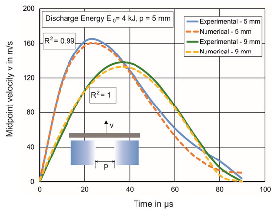
Figure 11.
Comparison of the vertical velocity of the midpoint of the workpiece from numerical and experimental (PDV) analyses for two different spacings (p) between the coils.
3.1.3. Comparison of the FEMM and LS-DYNA Model
The numerical model of FEMM was verified for use in further analysis by comparison of the current density with that obtained from the numerical model in LS-DYNA. This comparison is shown in Figure 12. The values predicted by the numerical model in LS-DYNA are slightly lower because of the actual damped current input, while FEMM can only account for a constant amplitude sinusoidal current. However, the current density obtained from FEMM contains many data points, lowering the requirement for interpolation between two calculated data. The current density from LS-DYNA is discrete and has only five data points.
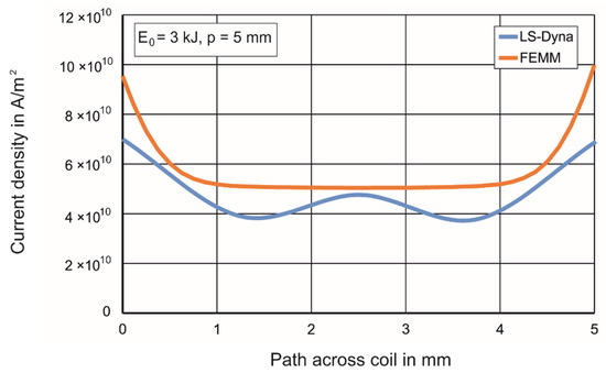
Figure 12.
Comparison of the current density distribution along the path from numerical models in LS-DYNA and FEMM. The data from LS-DYNA is very discrete and not a smooth curve, as shown in the graph.
3.2. Deformation of the Coils
3.2.1. Coil Deformation for Various Discharge Energies
Even though the coils were assigned as deformable solid bodies in the numerical model, the deformation obtained from the numerical model was much smaller than the experimentally measured deformation. In this section, the experimentally measured coil deformations are addressed.
The coils were fixed to the setup at both ends, as shown in Figure 7. Apart from this constraint, the coils were permitted to deform freely in all directions. Due to the current flowing in the same direction, the coils exert an attractive force towards one another. Based on the Ampère’s circuital law, the force per unit length between two parallel infinitely long wires is given in Equation (3), where the currents in the wires are given by and and the spacing between the wires is :
There is an inverse dependence of the force on the distance between the coils. For particular discharge energy, Figure 13 shows the displacement of the coils towards another. It is observed that as the spacing between the coils is increased, the displacement of the coil is reduced. This is because of the reduction of attractive Lorentz forces between the coils. For the discharge of 5 kJ, the 5 mm spacing causes the coils to displace to such an extent that a collision and repulsion of the coils occurs, leading to a different final shape. No conclusions can be made about the force between the two coils as plastic deformation of the coils takes place, and due to varying temperatures and strain rates, no direct relation between the force and displacements can be deduced. The figure helps in the qualitative understanding of the dependence of the coil displacement on the spacing between them.
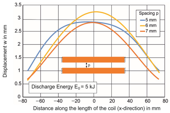
Figure 13.
Experimentally measured deformation of the coil along the coil length towards one another in x-direction due to attractive Lorentz forces for three different coil spacings. The coordinate directions are shown in Figure 2.
3.2.2. Coil Deformation for Various Cross-Sections
Due to the volumetric Lorentz force, the coil experiences a distributed load, which causes bending. This bending can be reduced by increasing the cross-section of the coil, as that increases the moment of inertia of the coil. In the experimental results explained in Section 3.2.1, the coil cross-section used was 5 mm × 5 mm. Two other cross-sections, shown in Figure 8, were analyzed experimentally. Figure 14 shows the displacement of the coils towards one another for the smallest cross-section and for the 10 mm × 5 mm one. The advantage of the 5 mm × 10 mm cross-section is that the moment of inertia when bending due to the attractive force of the other coil is much higher (4 times) than the other cross-section. This leads to a reduction in coil deformation. In the wider coil, the “effective distance” between the currents is higher due to the proximity effect, as the current migrates to the extremities of the coil cross-section. Figure 14 shows the comparison between the cross-sections 10 mm × 5 mm and 5 mm × 10 mm for the same values of discharge energy and spacing.
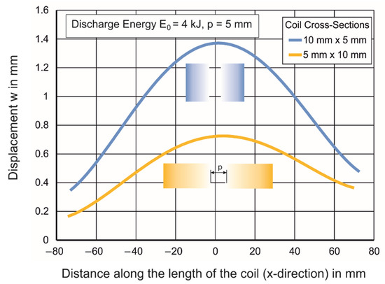
Figure 14.
Experimentally measured displacement of the coils in the y-direction for two different coil cross-sections.
4. Discussion
4.1. Deformation of the Sheet
4.1.1. Variation of Displacement, Midpoint Velocity and Efficiency of the Process with Coil Spacing
The deformation of the sheet was examined using the verified numerical model. Path 2, along which the deformation was examined, is shown in Figure 9. In the simulations with two coils, the displacement of the midpoint of the workpiece happens due to the combined influence of the Lorentz force applied by the two coils and the inertia of the workpiece. To examine the effect of the coil spacing between the final workpiece geometry, the discharge energy was kept constant. For a discharge energy of 4 kJ, the impact of spacing is shown in Figure 15. It is observed that the deformation of the apex of the workpiece is reduced with increasing coil spacing.
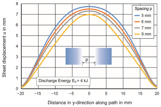
Figure 15.
Experimentally measured displacement of the workpiece in z-direction along path 2.
While the current remains the same, this deformation is explained by the reduction of the magnetic field intensity and, therefore, of the Lorentz force at the midpoint. The magnetic field intensity is smaller at the midpoint as the coils are further away for larger spacings, and it is inversely proportional to the distance. Figure 16 shows the magnetic field at the midpoint of the gap for various coil spacings, including those, which were not possible in the experiments due to design limitations.
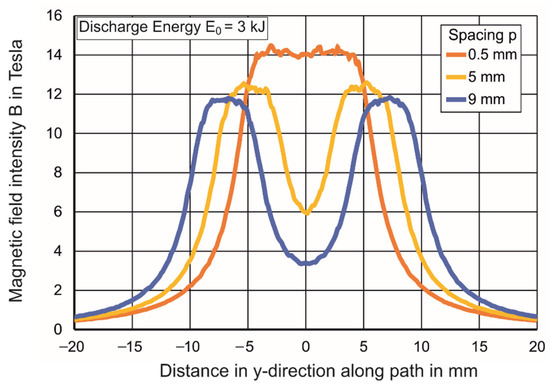
Figure 16.
Numerically determined magnetic field intensity along path 2.
In the case of the wider spacings, due to the low magnetic pressure at the midpoint, the maximum kinetic energy of the sheet at the midpoint is also low. Selected midpoint velocities obtained from the numerical model are presented in Figure 17. When the spacing is increased, the maximum velocity of the midpoint is reduced but saturates at greater values of coil spacing. The increase in spacing causes similar maximum velocity for the apex but with smaller acceleration. The reason for the lower velocity is not any difference in the circuit properties, and the current curves were also compared and determined to be highly similar. As for the lower spacing, the midpoint is located closer to the coils; the applied Lorentz force is higher, leading to higher acceleration. As the discharge energy is the same, a higher spacing causes less energy to be transferred to the midpoint and more to the local area just above the coil. The midpoint velocity saturates as it becomes a resultant of the inertia of the sheet rather than accelerating due to direct force application.
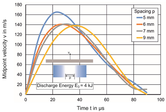
Figure 17.
Comparison of experimentally measured vertical midpoint velocity for four different coil spacings.
The efficiency of the process () can be calculated as the ratio of the energy used for forming the workpiece and the total energy discharge. The energy used for forming the workpiece is obtained from the simulations by integration of the plastic energy density (Equivalent strain times the flow stress) over the whole part volume at the end of the process. These efficiencies are typically very low, as more than half of the supplied energy is lost as Joule heat, according to Gies [7]. The efficiency is also dependent on the design of the setup and may be low because of the small size of the die cavity than the length of the coils. For the same setup and discharge energy, the efficiency of the process was observed to be related to the spacing between the coils. This dependency is observed in Figure 18 for different values of discharge energy.
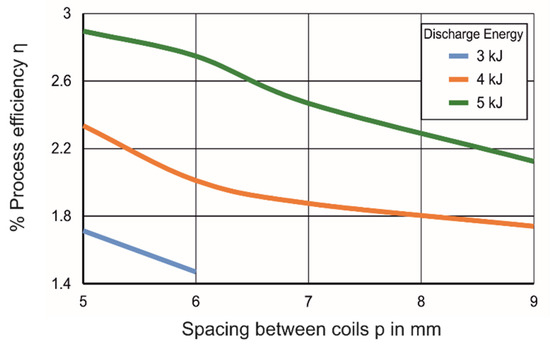
Figure 18.
Reduction in process efficiency for various values of coil spacings. The overall process efficiency increases as the discharge energy increases.
When the discharge energy is the same, the reason for a lower efficiency is the improper conversion of the supplied energy into the kinetic energy of the workpiece. The maximum kinetic energy of the workpiece was investigated during the process and analyzed for varying spacings between the coils. While the velocity was analyzed for just the midpoint, the maximum kinetic energy was monitored for the entire workpiece. It was seen that for the same discharge energy, the kinetic energy of the workpiece reduces with increased spacing between the coils from 5 mm to 9 mm by 22% for a discharge of 4 kJ energy and 26% for a discharge of 5 kJ energy. As a fraction of this kinetic energy is converted into the energy to deform the workpiece plastically, this energy reduces with increased spacing as well. The kinetic energy not converted to plastic work must get dissipated finally as heat along with other losses, such as friction.
4.1.2. Change of Local Curvature with Coil Proximity
The concentration of the current at the extreme periphery of the coil due to the proximity effect affects the quality of the workpiece as well. This effect is not explicitly visible when the displacement of the sheet is plotted, as shown in Figure 19. For the same discharge energy but various values of spacing, the local curvature of the sheet was calculated along path 2, shown in Figure 9 at the end of the process. The curvature () may be considered as a local bending-cum-stretching of the sheet, and it is defined as the inverse of the local radius. The curvature is calculated using Equation (4) and is plotted for two values of spacing in Figure 19. If the deformed contour of the workpiece is defined as and its spatial derivatives as and is as defined in Equation (4):
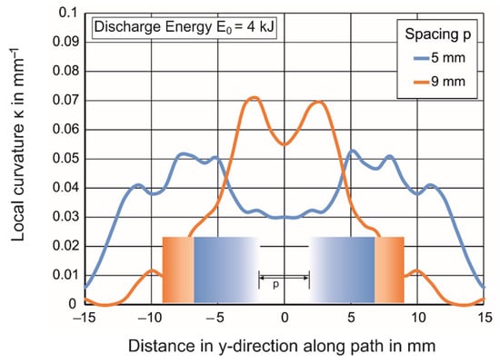
Figure 19.
Change in local workpiece curvature for coil spacings of 5 mm and 9 mm.
When the coils are close to one another, as is the case is for 5 mm spacing, the current migrates to the extremes. This high current density at the extreme applies a local pressure on the sheet and causes high bending in the region around it. This effect is much lower when the spacing is higher. Due to most of the current flowing along the top surface, the Lorentz force applied by the skewed current distribution causes a high local curvature of the sheet. When the current is almost uniform on the top surface, as for the case with higher values of spacing, one observes the bending localized at the midpoint (y = 0). This happens in the absence of large localized current densities, which bend the sheet locally.
4.2. Deformation of the Coils
4.2.1. Numerical Prediction of Force between Two Coils
To predict the total force between the two coils, the FEMM simulations were used. The assumptions used here were the following:
- No displacement of the coils and workpiece: As the force is applied, the coils begin to displace first elastically and then plastically towards one another. As the spacing between the coils is changed, it has an effect on the force as well, which will be higher than the predicted value. However, the displacement of the coils must start after a significant portion of the current is already discharged and must happen mostly due to inertia. Furthermore, according to Beerwald [26], most of the energy is transferred in the first two large pressure pulses of the current, until which, not much displacement of the coil is expected.
- An assumption about discharge current: FEMM can only model the discharge of a constant amplitude sinusoidal current, while the real current is damped in nature. Therefore, FEMM is used only for the calculation of the maximum force between the two coils, which would happen at the maximum value of current flowing between the two coils.
For the calculation of the Lorentz force between the two coils, FEMM uses Maxwell’s equations, which provide the Lorentz force exerted per unit volume. This is then multiplied to the volume of the element, and a vector addition for all elements is performed to give the overall force exerted. For various values of spacing, the force between the two coils is shown in Figure 20. The diagram is divided into two parts based on how well the diagram conforms to Equation (3), predicting the force between the two parallel current-conducting wires. For higher values of spacing, the force between the two coils follows Equation (3), and the conductors act as isolated from one another. For smaller values of spacing, the Equation (3) rule is abandoned. The force between the coils is much smaller than predicted by the equation rule. This is due to the redistribution of the current in the cross-section. Equation (3) assumes a uniform distribution of current in the cross-section. As the spacing decreases to small values, the current locates itself in the furthest end of the cross-section of the conductor, which leads to increased “effective distance” between the currents, and therefore, to a reduction of force.
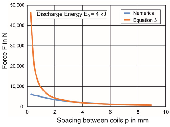
Figure 20.
Comparison of total force between two coils predicted by the numerical model in FEMM and the 1/r rule.
4.2.2. Measures to Avoid Coil Deformation
The deformation of the tool coil must be avoided in a real application to increase its reuse. To reduce coil deformation, the following measures are recommended:
- Changing the coil cross-section: Increasing the coil cross-section leads to lower deformations due to increased coil rigidity. However, the increase in dimensions of the cross-section leads to a lower current density and smaller workpiece deformation. Furthermore, if the width of the coil is increased to protect against the deformation due to the attractive force from the other coils, this will not provide much benefit against the reaction force exerted by the coil, which is orthogonal to the former force and about four times the magnitude in the geometry used in this study. It also increases the material used for the coils.
- Providing insulation support: In some of the experiments, the coils were separated by insulation made of glass-fiber-reinforced polymer, which has excellent compressive strength and insulating properties. In such experiments, the coil deformation due to the attractive force could be completely avoided. However, this led to a higher deformation in the orthogonal direction (the direction where the coil deformed due to the reaction force from the workpiece). With a good insulation design, the deformation of the coil can be completely avoided. Before implementation, however, the damping characteristics of the polymer must also be investigated.
- Innovative coil design: Gies [27] proposed using hybrid conductors for the reduction of coil deformation and suggested the methodology for the design as well. With the appropriate design of the steel support, plastic deformation of the coil can be avoided for some discharge energies. Other ideas for an improvement of the coil design could be the addition of cooling possibilities in the coil so that thermal softening of the material is prevented.
5. Conclusions
In this study, the spacing between the coil and the workpiece and the coil windings themselves was examined from multiple perspectives. Our objective was to understand and quantify the various phenomena when EMF is performed using conductors having multiple discrete turns. For this study, numerical and experimental methods were employed. The effect of spacing between coil turns on the overall workpiece displacement, workpiece midpoint velocity, efficiency and local curvature were observed. It was found that due to the proximity effect, the local curvature of the sheet is high for smaller spacings between the coils. Increasing the spacing reduces the process efficiency. For the coils, it was observed that the (undesired) deformation and the corresponding force between them both increase with reducing the spacing.
Generally, for parts with larger forming heights and high desired process efficiency, it is recommended to reduce the proximity between the coils. However, as the proximity between the coils is reduced, the forces between the coils increase, potentially leading to coil failure. Thus, there exists a tradeoff between process efficiency and tool life. The tool life may be increased by using coils with larger cross-sections and appropriate orientation.
As the spacing between the coils is an input parameter, it is essential to understand these phenomena and implement them in the setup design to obtain reliable results from EMF. Other results, such as the possible deformation of the coils, must be considered for a specific setup. For general safety of the tool coil, some recommendations, such as supporting the coil using rigid insulation and the potential addition of steel supports, are provided. Future studies in the prevention of tool coil deformation will focus on such hybrid coils.
Author Contributions
Conceptualization, S.P.G., M.L. and A.E.T.; methodology, S.P.G. and M.L.; software, S.P.G.; validation, S.P.G., A.E. and M.L.; formal analysis, S.P.G. and M.L.; investigation, S.P.G., A.E. and M.L.; resources, A.E.T. and M.H.; data curation, S.P.G. and M.H.; writing—original draft preparation, S.P.G.; writing—review and editing, S.P.G., M.H. and A.E.T.; visualization, S.P.G.; supervision, M.H. and A.E.T.; project administration, M.H. and A.E.T.; funding acquisition, M.H. and A.E.T. All authors have read and agreed to the published version of the manuscript.
Funding
This research was funded by the Deutsche Forschungsgemeinschaft (DFG) under project number 259797904. The authors express their gratitude and appreciate their commitment to support research.
Data Availability Statement
Not applicable.
Conflicts of Interest
The authors declare no conflict of interest.
References
- Psyk, V.; Risch, D.; Kinsey, B.L.; Tekkaya, A.E.; Kleiner, M. Electromagnetic forming—A review. J. Mater. Process. Technol. 2011, 211, 787–829. [Google Scholar] [CrossRef]
- Ahmed, M.; Panthi, S.K.; Ramakrishnan, N.; Jha, A.K.; Yegneswaran, A.H.; Dasgupta, R.; Ahmed, S. Alternative flat coil design for electromagnetic forming using FEM. Trans. Nonferrous Met. Soc. China 2010, 21, 618–625. [Google Scholar] [CrossRef]
- Demir, O.K.; Goyal, S.P.; Hahn, M.; Tekkaya, A.E. Novel Approach and Interpretation for the Determination of Electromagnetic Forming Limits. Materials 2020, 13, 4175. [Google Scholar] [CrossRef] [PubMed]
- Thibaudeau, E.; Kinsey, B.L. Analytical design and experimental validation of uniform pressure actuator for electromagnetic forming and welding. J. Mater. Process. Technol. 2015, 215, 251–263. [Google Scholar] [CrossRef]
- Gayakwad, D.; Dargar, M.K.; Sharma, P.K.; Purohit, R.; Rana, R.S. A Review on Electromagnetic Forming Process. Procedia Mater. Sci. 2014, 6, 520–527. [Google Scholar] [CrossRef]
- Takatsu, N.; Kato, M.; Sato, K.; Tobe, T. High-Speed Forming of Metal Sheets by Electromagnetic Force. JSME Int. J. 1988, 31, 142–148. [Google Scholar] [CrossRef]
- Gies, S.; Tekkaya, A.E. Effect of workpiece deformation on Joule heat losses in electromagnetic forming coils. Procedia Eng. 2017, 207, 347–346. [Google Scholar] [CrossRef]
- Golovashchenko, S.F. Material Formability and Coil Design in Electromagnetic Forming. J. Mater. Eng. Perform. 2007, 16, 314–320. [Google Scholar] [CrossRef]
- Taebi, F.; Demir, O.K.; Stiemer, M.; Psyk, V.; Kwiatkowski, L.; Brosius, A.; Blum, H.; Tekkaya, A.E. Dynamic forming limits and numerical optimization of combined quasi-static and impulse metal forming. Comput. Mater. Sci. 2012, 54, 293–302. [Google Scholar] [CrossRef]
- Watanabe, M.; Kumai, S. High-Speed Deformation and Collision Behavior of Pure Aluminum Plates in Magnetic Pulse Welding. Mater. Trans. 2009, 50, 2035–2042. [Google Scholar] [CrossRef]
- Dwight, H.B. Skin effect in tubular and flat conductors. Trans. Am. Inst. Electr. Eng. 1918, XXXVII-2, 1379–1403. [Google Scholar] [CrossRef]
- Kennelly, A.E.; Laws, F.; Pierce, P. Experimental researches on skin effect in conductors. Trans. Am. Inst. Electr. Eng. 1915, 34, 1953–2021. [Google Scholar] [CrossRef]
- Reatti, A.; Grasso, F. Solid and Litz-wire winding non-linear resistance comparison. In Proceedings of the 43rd IEEE Midwest Symposium on Circuits and Systems (Cat.No.CH37144), Lansing, MI, USA, 8–11 August 2000; pp. 466–469. [Google Scholar]
- Sigg, H.J.; Strutt, M.J.O. Skin effect and proximity effect in polyphase systems of rectangular conductors calculated on an RC network. IEEE Trans. Power App. Syst. 1970, 89, 470–477. [Google Scholar] [CrossRef]
- Popovic, Z.; Popovic, B.D. Introductory Electromagnetics; Prentice Hall: Upper Saddle River, NJ, USA, 2000. [Google Scholar]
- Riba, J.R. Calculation of the ac to dc resistance ratio of conductive nonmagnetic straight conductors by applying FEM simulations. Eur. J. Phys. 2000, 36. [Google Scholar] [CrossRef]
- Abdelbagi, H.E. Skin and Proximity Effects in Two Parallel Plates. 2007. Available online: https://corescholar.libraries.wright.edu/etd_all/18419 (accessed on 30 November 2020).
- Vitelli, M. Numerical evaluation of 2-D proximity effect conductor losses. IEEE Trans. Power Deliv. 2004, 19, 1291–1298. [Google Scholar] [CrossRef]
- L’Eplattenier, P.; Cook, G.; Ashcraft, C.; Burger, M.; Imbert, J.; Worswick, M. Introduction of an Electromagnetism Module in LS-DYNA for Coupled Mechanical-Thermal-Electromagnetic Simulations. Steel Res. Int. 2009, 80, 351–358. [Google Scholar] [CrossRef]
- Gies, S.; Tekkaya, A.E. Analytical prediction of Joule heat losses in electromagnetic forming coils. J. Mater. Process. Technol. 2017, 246, 102–115. [Google Scholar] [CrossRef]
- Liu, X.; Huang, L.; Su, H.; Ma, F.; Li, J. Comparative Research on the Rebound Effect in Direct Electromagnetic Forming and Indirect Electromagnetic Forming with an Elastic Medium. Materials 2018, 11, 1450. [Google Scholar] [CrossRef] [PubMed]
- Weddeling, C. Electromagnetic Form-Fit Joining. Ph.D. Dissertation, Universität Dortmund, Dortmund, Germany, 2014. [Google Scholar]
- Clausen, A.H.; Børvik, T.; Hopperstad, O.S.; Benallal, A. Flow and fracture characteristics of aluminium alloy AA5083–H116 as function of strain rate, temperature and triaxiality. Mater. Sci. Eng. A 2004, 364, 260–272. [Google Scholar] [CrossRef]
- Kabirian, F.; Khan, A.S.; Pandey, A. Negative to positive strain rate sensitivity in 5xxx series aluminum alloys: Experiment and constitutive modeling. Int. J. Plast. 2014, 55, 232–246. [Google Scholar] [CrossRef]
- Moro, E.A. New Developments in photon Doppler velocimetry. J. Phys. Conf. Ser. 2014, 500, 142023. [Google Scholar] [CrossRef]
- Beerwald, C. Grundlagen der Prozessauslegung und -Gestaltung Bei der Elektromagnetischen Umformung. Ph.D. Dissertation, Universität Dortmund, Dortmund, Germany, 2005. [Google Scholar]
- Gies, S.; Tekkaya, A.E. Design of Hybrid Conductors for Electromagnetic Forming Coils. In Proceedings of the 8th International Conference on High Speed Forming, Columbus, OH, USA, 14 May 2018. [Google Scholar] [CrossRef]


Publisher’s Note: MDPI stays neutral with regard to jurisdictional claims in published maps and institutional affiliations. |
© 2021 by the authors. Licensee MDPI, Basel, Switzerland. This article is an open access article distributed under the terms and conditions of the Creative Commons Attribution (CC BY) license (https://creativecommons.org/licenses/by/4.0/).