Article

3D Thermal Simulation of a Laser Drilling Process with Meshfree Methods

by
Mohamadreza Afrasiabi
1,2,* and
Konrad Wegener
2
1
Chair of Structural Mechanics & Monitoring, ETH Zurich, Stefano-Franscini-Plz 5, 8093 Zurich, Switzerland
2
Institute of Machine Tools & Manufacturing, ETH Zurich, Leonhardstr. 21, 8092 Zurich, Switzerland
*
Author to whom correspondence should be addressed.
J. Manuf. Mater. Process. 2020, 4(2), 58; https://doi.org/10.3390/jmmp4020058
Submission received: 24 May 2020 / Revised: 16 June 2020 / Accepted: 19 June 2020 / Published: 22 June 2020
(This article belongs to the Special Issue Optimization and Simulation of Solid State Manufacturing Processes)

Abstract

:
Numerical simulation of laser drilling is rapidly gaining interest in academia and industry since this process remains one of the most important and widely-used technologies in modern manufacturing. Meshfree methods such as Smoothed Particle Hydrodynamics (SPH) have proven to be successful as a numerical tool for the computation of the heat transfer and material removal associated with a laser drilling problem. Nonetheless, the vast majority of recent developments incorporate an inconsistent SPH kernel into their thermal simulations. In this paper, several enhanced schemes are implemented to address this problem by solving the heat transfer more accurately. These meshfree schemes can provide a second-order accurate discretization of the Laplace operator and abolish the inconsistency issue of the standard SPH kernels. An efficient approach is additionally suggested to handle the associated boundary conditions, which relies on the idea of the color function and particle label. The implementation is initially validated by a 3D benchmark study and then applied for the first time to a laser drilling problem.

1. Introduction

Laser drilling is a manufacturing process where pulsing laser beams are focused on a workpiece to create popped holes (also known as thru-holes). Due to their unique efficiency and accuracy, these technologies have become the center of attraction in various fields of application such as the gas turbine, aerospace, and printed circuit board industries. The analysis of a laser drilling problem is typically governed by an energy balance, where the thermal energy provided by a focused laser beam is conducted into the workpiece and consumed to melt or vaporize the material. This description indicates that solving the heat equation for solids is of crucial concern for the analysis of laser drilling problems since thermal effects are usually the prevalent mechanism during such processes. In brief, there exists a wide range of physical phenomena (including the thermal issues), process variables, and material parameters in laser manufacturing, recognized as the main complexities for its theoretical and experimental developments.
Numerical modeling, on the other hand, is an alternative approach that can leverage the improvement potentials of laser drilling processes. Reliable computational models are valuable tools for the characterization of quantities that are impossible to predict by theory and/or extremely hard/expensive to measure in experiments. From this point of view, laser drilling problems seem to be a prime candidate for numerical simulation since they are typically involved in ultra-fast pulses and abrupt phase changes [1,2]. According to hundreds of scientific citations, the Finite Element Method (FEM) may be regarded currently as the tool-of-choice in the domain of laser processing simulations. Examples include the FEM model designed for high energy lasers by [1], the investigation of temperature fields in sheet metals [3], the modeling of the laser welding process in butt-joint specimens [4], and the simulation of fundamental laser-micromachining processes [5]. While the use of the Finite Difference Method (FDM) [2] and the Finite Volume Method (FVM) [6] can also be found in the literature, it is hard to overstate the superiority of FEM over other mesh-based manufacturing simulations.
Another class of spatial discretization is based on particles (instead of a mesh), which is found to be a particularly promising approach for applications with complex free-surfaces, phase changes, and multiple material interfaces. The simulation of laser-based manufacturing technologies in general, and laser drilling in particular, encounters all these difficulties to a considerable extent. Therefore, several researchers have attempted to investigate the performance of meshfree particle methods in laser-based manufacturing simulations. In 2008, Gross [7] introduced a first version of the Smoothed Particle Hydrodynamics (SPH) model for modeling a simple laser cutting process. Later, an SPH thermal model of the direct laser interference patterning was developed by [8]. In the article published by Kim [9], Isoparametric Finite Point Interpolation (IPIM) techniques in both weak and strong forms were applied to simulate the material removal process in laser drilling. These early studies demonstrated an enormous potential of meshfree methods in simulating laser manufacturing processes.
More recent works include the 3D laser cutting simulation by [10] using a commercial SPH package and an improved SPH formulation for heat transfer in the laser ablation of aluminum [11]. Other interesting efforts, more closely falling into the scope of this paper, are the application of the Radial Point Interpolation Method (RPIM) [12] and the Meshless Local Petrov–Galerkin (MLPG) collocation method [13] for the heat conduction in laser drilling. In [14], the authors reproduced the results of [12] by using yet another particle-based scheme. It is worth mentioning that the number of SPH developments in other fields of application is overwhelming, and numerous efforts have been made to model a variety of structural [15], CFD [16,17], and manufacturing simulations [18,19,20,21], to name a few. While a growing share of interest in meshfree simulations of laser processing can be noticed upon this literature survey, a comprehensive study of higher order SPH formulations for (3D) thermal modeling in laser-based manufacturing processes seems to be missing from the current state-of-the-art.
Thus, the ultimate goal is to develop a highly efficient and robust meshfree solver that can provide a design tool for laser-based manufacturing models including all thermal-mechanical-material coupling effects. In the pursuit of a framework with such capabilities, this work sets its sights on the development of a robust 3D thermal solver for laser drilling applications. The first application of the methods listed in Table 1 to the heat transfer simulation of a laser drilling model is presented. Furthermore, an efficient strategy for handling the boundary issues is suggested, which relies on the idea of the color function and particle label. We also highlight the use of more advanced SPH formulations to recover first- and second-order consistency for the Laplace operator. This contribution allows for a more accurate solution of the heat equation, especially in the presence of complex boundary conditions. After validating the computer implementation in a 3D benchmark test, the proposed framework is subsequently utilized to simulate a laser drilling process.
The remainder of this paper is organized as follows. In Section 2, the relevant physics is described in some detail, including the more important of the simplifications employed by multiple research groups active in the field. Section 3 is the core of this article, where the selected meshfree methods are presented in such a way that they can be implemented in computer code with minimum effort. In Section 4, the numerical simulation framework is first validated by performing a convergence study and then applied to the laser drilling process. Concluding remarks are presented in Section 5.

2. Laser Drilling Model

A graphical illustration of the laser drilling process is displayed in Figure 1, where a laser beam is acting on a metallic material. As can be viewed in this figure and according to [28], laser drilling of cylindrical holes generally occurs through the melting and vaporization of the work material, plus the auxiliary action of the assist gas. In such a process, the focused laser beam serves as the external source providing the energy required to remove material. On the other hand, the assist gas facilitates the drilling process via an exothermic reaction (usually with oxygen) and/or evacuates molten material from the popped hole.

2.1. Problem Statement

A complete physical model of such processes is far from simple and would warrant original research as it needs to resolve multiple challenging issues including new surface generation, different time and length scales, and multiple material-phase interfaces with extreme and complex movement. In this paper, the diverse range of physical phenomena governing laser drilling processes is reduced to a thermal simulation in solids such that the present numerical solver can be applied effectively. In what follows, the details of the underlying physical model are described.
In our simplified model, a static laser beam source with a μ s to ms pulse duration is considered, while the assist gas is not modeled in the thermal analysis. The single-pulsed laser used here has a pulse duration of 150 μ s and a peak power of 100 W exerted on a very thin sheet metal made of stainless steel with a thickness of less than 200 μ m. Given these situations, a set of simplifying assumptions is outlined in the following similar to the reference model introduced by [10,13].
  • The material is isotropic and homogeneous with constant thermo-physical characteristics.
  • The input laser follows a Gaussian beam distribution and is considered to be a surface heat flux.
  • The laser beam is absorbed on the surface and emitted vertically downward. The absorptivity coefficient is taken to be constant and describes the absorbed power over the surface projected in the direction of the laser beam.
  • The laser beam radius is constant (=beam waist).
  • The melt flow, plasma formation, and recoil pressure are not considered in the model.
  • The molten material point is removed as soon as it reaches the melting temperature (without considering the latent heat) and does not show hydrodynamic behavior.
  • The removed material is transparent and does not absorb the laser energy.
The corollary to these simplifications is to allow for a single-phase thermal modeling of the laser drilling process.

2.2. Governing Equations

The thermal field is governed by the Fourier heat equation for isotropic solids expressed in a 3D Cartesian coordinate system as:
ρ c p T t = k 2 T = k 2 T x 2 + 2 T y 2 + 2 T z 2
where ρ is the density, c p specific heat capacity, T temperature, and k heat conductivity. The boundary conditions associated with Equation (1) are the surface heat flux terms defined as:
  • Heat source q s due to the absorbed laser beam.
  • Heat loss q l due to convection and radiation.
These terms are given by:
q s = n z a L P L π r b 2 exp 2 r r b 2
q l = h c ( T s T ) convection + ϵ σ ( T s 4 T 4 ) radiation
in which n z is the direction cosine of the normal vector outward from the laser-irradiated surface, a L the laser absorption coefficient ( 0 < a L < 1 ), P L the laser peak power, r the radial distance from the beam center, and r b the laser beam radius (i.e., in the waist). In Equation (3), h c is the heat convection coefficient, T s and T the surface and background temperatures, respectively, ϵ the emissivity factor, and σ the Stefan–Boltzmann constant.

3. Numerical Modeling

An overview of the numerical methods to be used for the thermal model described in Section 2 is the central focus of this section. For more clarity, the problem is decomposed into the following subsets.
  • Discretization of the Laplace operator in Equation (1).
  • Treatment of boundary conditions in Equations (2) and (3).
  • Time integration of Equation (1).
Details regarding the temporal discretization of an ODE in meshfree models are not provided in this paper. It suffices to point out that an explicit leapfrog stepping according to [29] is used for the time integration unless otherwise stated. It is widely accepted in explicit algorithms to impose a maximum step size Δ t for the sake of solution stability. In this work, the step size is calculated from the Courant–Friedrichs–Lewy (CFL) criterion by restricting the maximum permissible value of Δ t to obey:
Δ t χ ( Δ x ) 2 α
where Δ x is the characteristic distance between particles, α = k / ρ c p the thermal diffusivity, and χ a scale factor considered to be 0.25 in this paper. Discussions regarding the first and second parts of the problem decomposition are presented with more detail in the next two subsections.

3.1. Meshfree Schemes for Laplacian Approximation

The present framework requires no computational mesh for spatial discretizations and is built on the notion of SPH techniques. In principle, SPH is an interpolation method based on the position of Lagrangian particles and the use of a smooth weighting function called the kernel. Following the original derivation by [30,31], the numerical procedure of SPH for an arbitrary field f ( r ¯ ) at particle i consists of two approximations:
f ( r ¯ i ) f ( r ¯ i ) = Ω f ( r ¯ ) W ( | r ¯ i r ¯ | , h ) d V kernel approximation ( interpolation )
f ( r ¯ i ) j f ( r ¯ j ) W ( | r ¯ i r ¯ j | , h ) V j particle approximation ( discretization )
where Ω is the computational domain, d V a differential volume element, and W a kernel function that depends only on two variables: the particle distance r ¯ i j = | r ¯ i j | = | r ¯ i r ¯ j | and the smoothing length h. A variety of frequently-used kernels in SPH models were listed in [29,32], from which the following functions were chosen for the numerical examples of this paper.
  • Cubic B-spline:
    W h ( r ¯ ) = n c × 1 3 2 q 2 + 3 4 q 3 , 0 q < 1 1 4 ( 2 q ) 3 , 1 q 2 0 , otherwise
  • Wendland quintic:
    W h ( r ¯ ) = n c × ( 1 q 2 ) 4 ( 2 q + 1 ) , q < 2 0 , otherwise
where r is the position vector, h the smoothing length, which controls the amount of mollification (smoothing), and q = | r ¯ | / h . The normalization constant for 3D space is n c = 1 / π h 3 and n c = 21 / 16 π h 3 for the cubic B-spline and Wendland quintic kernels, respectively.
A major novelty of this article lies in the first application of these methods to the (3D) laser drilling problem, while the 3D implementation of ICSPM is presented for the first time. Without delving deeply into their derivations, the six variants listed in Table 1 of the introductory section are reviewed in consistent notation and a self-contained fashion.

3.1.1. Brookshaw’s Approximation (BSH)

The method presented by Brookshaw [22] is considered as one of the most popular options in SPH implementations. It benefits from a simple correction to the original SPH form and is expressed by:
2 T i BSH j 2 T i T j | r i j | e ¯ i j · W i j V j
where e ¯ i j = r ¯ i j / | r i j | is a unit vector in the inter-particle direction. BSH guarantees the conservation of energy to the precision of the time-stepping algorithm, which is an important feature of this scheme.

3.1.2. Particle Strength Exchange (PSE)

Introduced by [23,33] for the Laplacian approximation of advection-diffusion problems, PSE is regarded as a strong numerical tool for solving diffusion problems. Instead of computing the derivatives of the same SPH kernel, PSE constructs different kernels for different derivatives independently. A good review of this method can be found in [34,35]. Discretization of the three-dimensional Laplacian of T using a second-order PSE kernel reads:
2 T i PSE j ( T j T i ) 1 h 3 4 π π h 2 exp ( | r ¯ i j | / h ) 2 V j
where the pre-factor 1 / h 3 appears due to the scaling property of PSE kernels in 3D geometries. A more exhaustive list of other PSE kernels for various differential operators and different dimensions can be found in the Appendix of [34]. A comparison between Equations (9) and (10) reveals that the PSE approximation also offers the conservation of energy up to the precision of the time-stepping algorithm. It is understood from Equations (9) and (10) that the Laplacian results using BSH and PSE are not generally consist because of their kernel deficiency near/on the boundaries. The corrective schemes presented in the next subsections are employed to address this issue.

3.1.3. Reproducing Kernel Particle Method (RKPM)

RKPM is a meshfree technique, which, in theory, can be derived for a favorable order of accuracy and consistency by incorporating different correction functions. In 1995, Liu et al. [24] originally applied this method in their seminal work to advection-diffusion problems. The constructive idea of RKPM is to enhance SPH kernels by applying a correction function ψ for recovering the consistency. Iterating the same procedure described in [35] for 3D implementations leads to a first-order consistent RKPM approximation for second derivatives, and subsequently, for the Laplace operator. If the approximation of 2 / x 2 for T is desired, the mathematical expression arrives at:
2 T i x 2 RKPM j T j 2 ψ i j x 2 W i j + 2 ψ i j x · W i j x + ψ i j 2 W i j x 2 V j
where ψ is a linear correction function whose unknown coefficients are determined by enforcing a set of moment conditions and solving a system of linear equations. This procedure is repeated for the other spatial coordinates to find the Laplacian value by summing three individual second derivatives (in 3D). As pointed out in [35], it is quite popular to utilize a symmetric or anti-symmetric form of Equation (11) by replacing T j with [ T j ± T i ] .

3.1.4. Corrective Smoothed Particle Method (CSPM)

CSPM was initially derived in [25], but presented later by Chen and Beraun [36] in a more generalized framework. The constructive idea of CSPM is to reduce errors in the first and second derivatives computed with SPH by correcting the gradient operators and manipulating the Taylor series expansion. For the calculation of the second derivatives in CSPM, the values of the first derivatives must be known beforehand. The CSPM discretization of the second derivatives involves multiple matrix operations and a system of linear equations for each particle at each time step. It can be written as:
T i CSPM B i 1 j ( T j T i ) W i j V j j r ¯ j i · T i W i j V j
T i A ~ i 1 j ( T j T i ) W i j V j
whereby the fourth-order tensor B is defined for particle i:
B i = j C ~ i j W i j V j
in which the expanded definition of matrix C ~ is found in [35,36], and the renormalization matrix A ~ for particle i is computed by:
A ~ i = j r ¯ j i W i j V j
It should be noted that T in Equation (12) indicates the Hessian matrix of T, meaning that the numerical value of 2 T still needs to be calculated by the sum of elements on the main diagonal. Chen et al. [25,37] showed that CSPM is a first-order consistent method that enhances the solution accuracy, not only near the boundary, but also inside the domain.

3.1.5. Improved CSPM

More recently, Korzilius et al. [27] showed that a second-order consistent discretization of the Laplace operator can be obtained by incorporating a discrete first derivative, which is second-order consistent. They included one more term in the corresponding Taylor series of T in Equation (13) and derived a new fourth-order renormalization tensor D for the second derivatives:
T i ICSPM D i 1 j ( T j T i ) W i j V j j r ¯ j i · T i W i j V j
where T i was defined in Equation (13) and D is calculated from:
D i = B i j ( r ¯ j i W i j ) V j · A ~ i · j ( C ~ i j W i j ) V j
Just like CSPM, the Laplacian value using ICSPM needs to be calculated by the sum of the elements on the main diagonal of Equation (16). The ICSPM approximation gives a second-order consistent solution [27], while its extra computational effort compared to CSPM is negligible. An adaptation of ICSPM for thermal modeling of 2D multi-phase flows was presented by [38].

3.1.6. Fatehi’s Meshfree Scheme (FMFS)

Originally derived by Fatehi et al. [26] and recently applied to 3D heat conduction problems in [35], FMFS is another modern SPH scheme that provides a second-order consistent approximation of the Laplace operator. It computes 2 of function T via:
2 T i FMFS G ~ i : j 2 ( T j T i ) | r ¯ i j | e ¯ i j · j V j ( T j T i ) A ~ i 1 · W i j e ¯ i j W i j V j
by introducing a novel second-order renormalization tensor G ~ computed from:
G ~ i : E ¯ ~ i · A ~ i 1 · F ¯ ~ i + j r ¯ i j e ¯ i j e ¯ i j W i j V j = I ~
in which “:” denotes the double contraction of two second-order tensors. The CSPM renormalization tensor A ~ was defined in Equation (15), and e ¯ i j = ( x ¯ i j + y ¯ i j + z ¯ i j ) / r i j is the normalized or unit vector. The terms E ~ and F ~ in Equation (19) are third-order tensors given by:   
E ¯ ~ i = j e ¯ i j e ¯ i j W i j V j
E ¯ ~ i = j r ¯ i j r ¯ i j W i j V j
which are sensitive only to the location of particles. In order to minimize the computational effort of this expensive method, it is beneficial to maximize the amount of pre-computation intensity. Because the particles’ location is the only ingredient that constitutes the correction terms and renormalization tensors, the pre-computation block (which appears in corrected SPH methods) needs to be called only if any changes occur to the particle arrangement. This statement applies to other corrected SPH methods as well.

3.2. Proposed Approach for Boundary Issues

A simple and efficient strategy is proposed for the identification of surface particles, which can be used for thermal modeling applications without material deformations. The rationale behind this approach is twofold: (1) to calculate the unit normal vector at the laser-irradiated surface; (2) to impose the boundary conditions defined in Equations (2) and (3) on surface particles at each time-step.
Since the source term q l is a surface heat flux, the direction cosine of the normal vector outward from the laser-irradiated surface, n z in Equation (2), needs to be known. Calculation of the unit normal vector in this work follows the color function idea used for the surface tension term in CFD applications [16,38]. For particle i:
n ¯ ^ i = n ¯ i | n ¯ i | c i | c i |
wherein n ¯ ^ is the unit normal vector and c the gradient of the color function calculated via a symmetric SPH approximation:
c i 1 V i j V i 2 + V j 2 c i i + c i j 2 W i j
with V being the integration volume of particles. This is in fact a density-weighted color function [16], in which the index number c i j between two different phases (or colors) is computed from:
c i j = 2 ρ i ρ i + ρ j if particle i and j belong to different phases / labels 0 if particle i and j belong to the same phase / label
Moreover, one notices that q l should be applied only to the laser-irradiated particles. A straightforward approach is suggested for detecting these surface particles during the simulation. It performs locally and makes use of a state flag for each particle. In summary, the order of operations is given in the following four steps.
  • Particle i is marked molten as soon as its temperature reaches the melting point.
  • The neighbor particles adjacent to particle i are marked with a candidate flag.
  • All candidate particles that are neither molten nor already surface particles become new surface particles.
  • All molten particles are deleted.
Clearly, this strategy is valid (and efficient) as long as particles are fixed in space and the array of particle positions remains unchanged in memory, ensuring a fast identification of the neighboring particles. Figure 2 illustrates how the proposed approach works at a given time-step. Due to symmetry and for the sake of better visualization, only half of the workpiece is displayed. It is readily apparent that this laser drilling problem has a high symmetry around the irradiation axis, hence is a 2D axisymmetric model. Nevertheless, the present simulation was run in 3D to verify the computer implementation and efficiency.

4. Results and Discussion

Before simulating the laser drilling model in this section, a validation benchmark on a 3D transient heat conduction problem was conducted to ensure the correct implementation of the presented methods. As for the computer software, the open-source code “Thermal-IWF” written in C99 and published by [35] is utilized. To download this solver, please refer to the https://github.com/mroethli/thermal_iwf repository. All computations were performed on an Intel ® Core™ i5-4690 with four processors at 3.50 GHz. Most of the images were created with ParaView [39]—a powerful visualization tool for large datasets.

4.1. Validation Benchmark

The test case was related to the time-dependence of temperature fields in a 3D object and examined the accuracy and performance of the Laplacian models presented in Section 3.1. If the initial condition of Equation (1) follows a thermal pulse at the origin of the domain ( x o , y o , z o ) without Dirichlet boundary conditions, the time-dependent analytical solution of this problem at time t can be computed from:
T = 1 ( 4 π α t ) ( 4 π α t ) exp | r | 2 4 α t
in which α is the thermal diffusivity assumed to be one in this model, | r | the radial distance from the origin, and T the temperature value at time t generated by an instantaneous source of heat at the origin point P o ( x o , y o , z o ) at time t = t 0 . The time span for the transition of heat in this mode was considered to start from t 0 = 0 . 1 and end at t f = 0 . 3 . The infinite boundaries were herein limited to a cube of x 5 , + 5 , y 5 , + 5 , z 5 , + 5 , as shown by the black outlined boxes in Figure 3. This domain size was deemed sufficiently large because the boundary temperature due to the heat impulse in the origin at t f would be about 10 19 , orders of magnitude less than the error due to the methods and, in fact, orders of magnitude smaller than the machine epsilon.
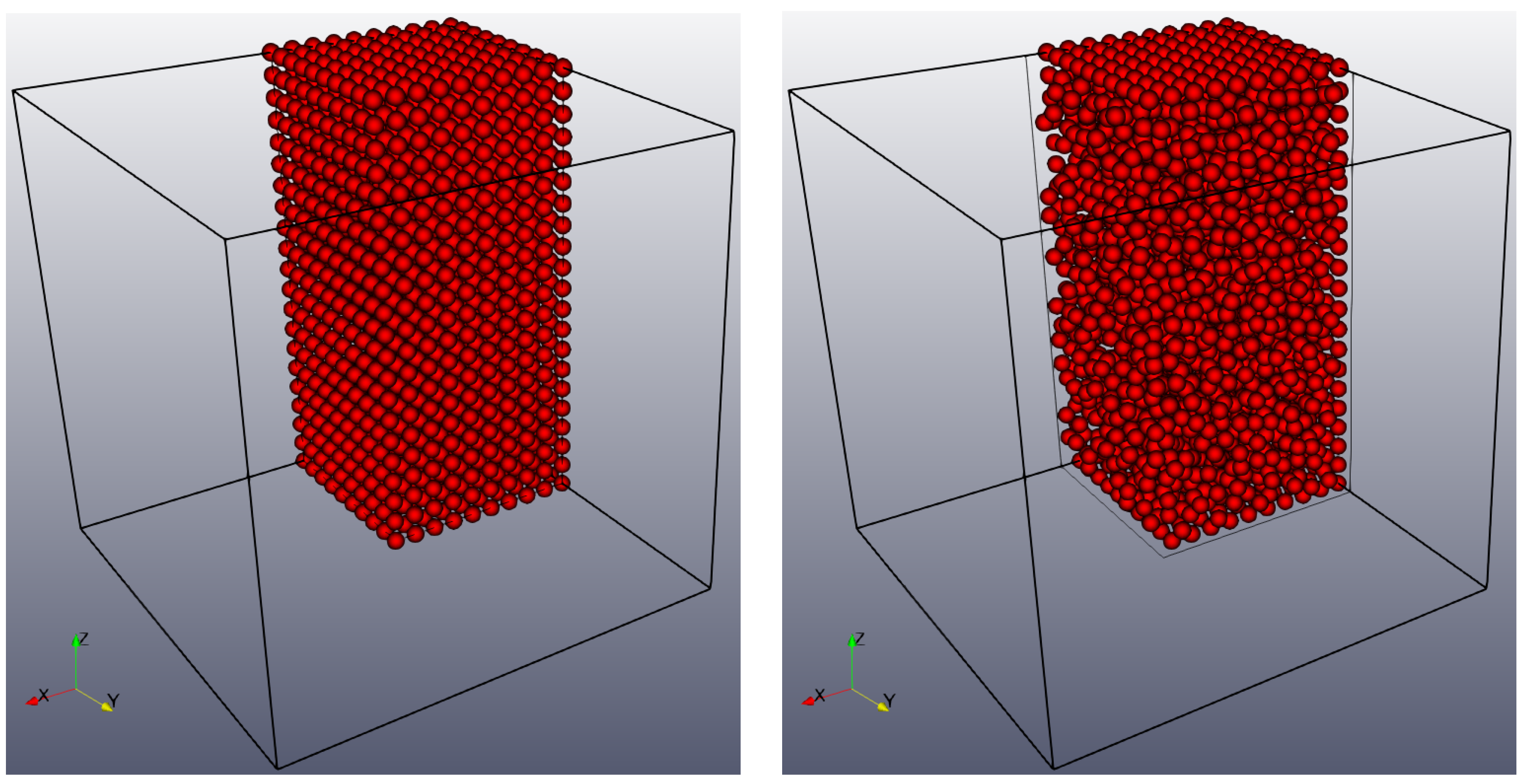
The particle spacing (i.e., discretization size) was chosen from Δ x = { 1 , 0 . 5 , 0 . 25 } to evaluate the errors and draw the convergence plots. All simulations were carried out on both regular and random particle arrangements to compare the capabilities of the methods in handling disordered situations. The randomness of particles was limited to the maximum of 50% inhomogeneity for all particles except from the edge points. The edge particles were always distributed with a regular spacing (see Figure 3).
The numerical results were compared with the exact solution at t f = 0 . 3 , and the L 2 
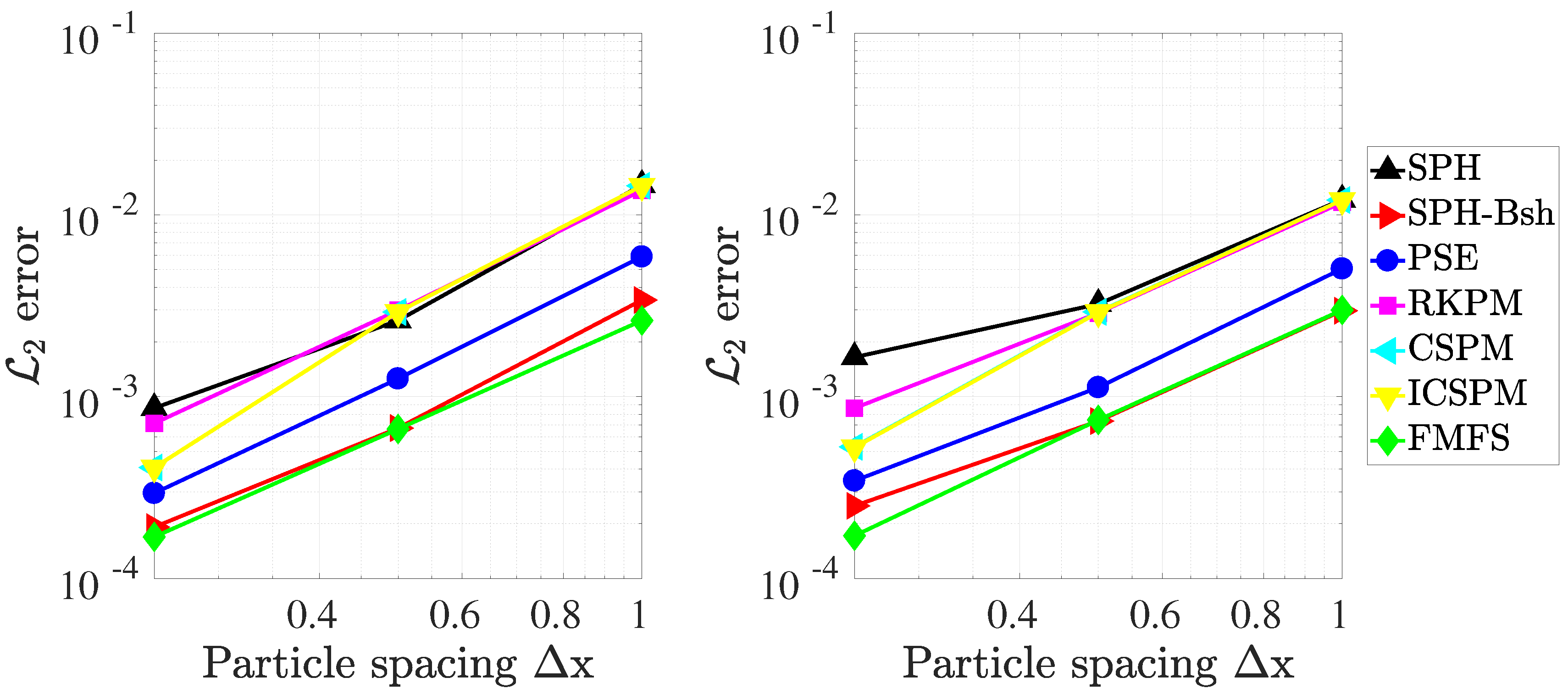
norm of the error is reported. The convergence plots shown in Figure 4 permit several interesting observations. Firstly, it can be seen that almost all methods converged with a second-order slope in the regular spacing (left graph in Figure 4). Secondly, CSPM and ICSPM delivered identical results for the uniform case. This was quite unsurprising because the main advantage of ICSPM over CSPM is its ability to provide higher-order consistency by improving the boundary deficiency, but the boundary effect in this example was negligible. When particles were not uniformly spaced, however, a marginal difference between the CSPM and ICSPM results was noticed. Thirdly, FMFS demonstrated the lowest error and outperformed the other Laplacian models in almost all cases. This was due to the higher order terms included in its truncation error. A particularly interesting conclusion from this investigation was the nearly identical behavior of SPH Brookshaw (the red graphs in Figure 4) and FMFS in discretizing the Laplacian term for uniform cases. The reason lied in the derivation process of FMFS, which originated from a Brookshaw approximation. Please consider [35] for more details in this regard.

4.2. Laser Drilling Simulation

The case study pertained to a sheet metal made of stainless steel (SS 316L) with a width of l x = 100 μ m, length of l y = 200 μ m, and thickness of l z = 150 μ m. Consistent with the initial configuration of the 3D model used by Muhammad et al. [10], the same material and laser properties were taken into account. Listed in Table 2 is a summary of the parameters used for this simulation. The absorptivity coefficient a L was chosen to be 40 % according to a very relevant investigation performed by [13] on the sensitivity of MLPG results to this parameter.
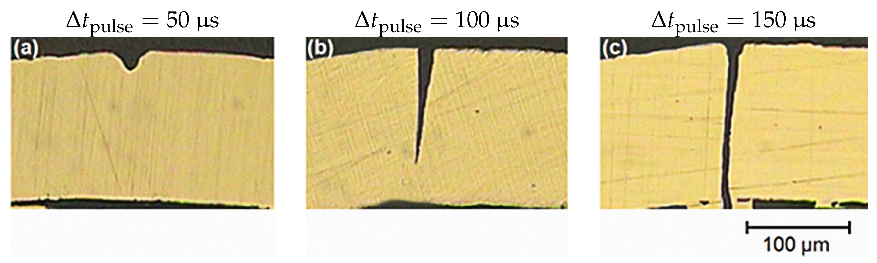
Muhammad et al. [10] were the first who considered this experimental setup for SPH modeling and showed that a pulse of 150 μ s could fully penetrate the metallic sheet with a thickness of 150 μ m. Three images adapted from the laser cutting experiments of [10] are presented in Figure 5 for three different pulse durations. As a result of this observation, the present thermal simulation was terminated at t = 150 μ s to investigate the computed temperature distribution, removed volume, and penetration depth.
Firstly, a parametric study of this example was carried out in 2 spatial resolutions using 2 kernel functions and 3 different smoothing lengths, for all 6 methods presented in Section 3.1. This combination led to a massive load of simulations including 72 configuration setups. The numerical results are inserted into Table 3, Table 4, Table 5 and Table 6, where quantities of three different kinds are reported for assessment:
  • The percentage of the volume removed from the workpiece after Δ t = 150 μ s if the total volume to be removed was conceptually equal to a cylinder of radius r b = 25 μ m and height l z = 150 μ m.
  • Whether or not a full penetration was observed.
  • The measured CPU runtime of the simulation.
The parameter Δ x in these four tables denotes the characteristic distance between particles in a uniform domain. Furthermore, the appearance of “—” corresponds to a scenario where the numerical result was unreliable or invalid. The source of these errors may stem from different issues such as the surface detection algorithm, boundary conditions, insufficient number of neighbor particles, and inconsistent kernels. An elaboration of how to resolve such issues is irrelevant to the scope of this paper and thus not provided. For further discussions, the readers are referred to textbooks and review articles such as [40,41]. Note that 2 T at surface particles was always computed by PSE even if other corrective schemes (RKPM, CSPM, ICSPM, or FMFS) were employed in the code. This new workaround ensured the stability of the solution without requiring exterior dummy particles for an invertible correction matrix where boundaries were not well defined geometrically (e.g., the laser-irradiated surface inside the popped hole).
As can be seen in these tables, CSPM and ICSPM showed the least stable behavior among the other schemes. This issue was due to the excessive number of inverse matrix calculations and also interrelated with the proposed boundary treatment approach. Unsurprisingly, the choice of the kernel function had a major impact on the stability of the simulation results. A comparison between Table 3 and Table 4 in the case of CSPM/ICSPM supported the argument that the cubic B-spline kernel performed weaker than its contestant at higher h. As a result, the Wendland quintic kernel function was selected for final simulations at a high resolution.
As far as the computational cost was concerned, attention must be paid when comparing the runtime of different schemes in purely thermal simulations. In all corrective methods (RKPM, CSPM, ICSPM, and FMFS), a significant proportion of the computational cost was attributed to the computation of their correction matrices. However, the evaluation of these matrices here was not updated within the main time loop, and a remarkable amount of computational time could be saved because the particle position remained unchanged during a purely thermal simulation. Interestingly though, the PSE scheme was indifferent to the movement of particles. It considered an exponential kernel according to Equation (10), no matter if the particle position had been changed or not. Therefore, any conclusive judgment about the computational performance of these six methods was reckoned to be inaccurate and was probably unfair.
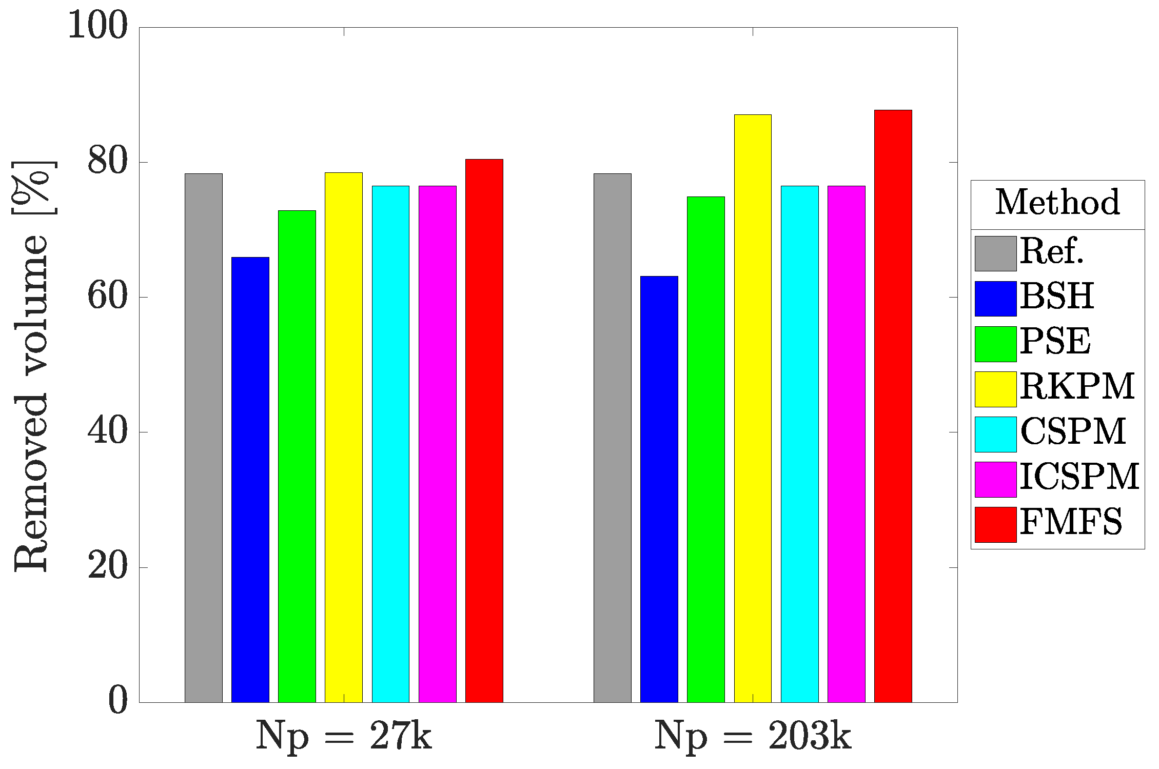
After having completed the parametric study, the optimum setup for each method could be configured. In Figure 6, the removed volume predicted by this 3D solver is compared to the corresponding value taken from a 2D meshless model developed by Abidou et al. [13]. The bar-chart shows that the highest volumes were computed by FMFS on account of its higher order terms involving a larger number of particles for each interpolation.
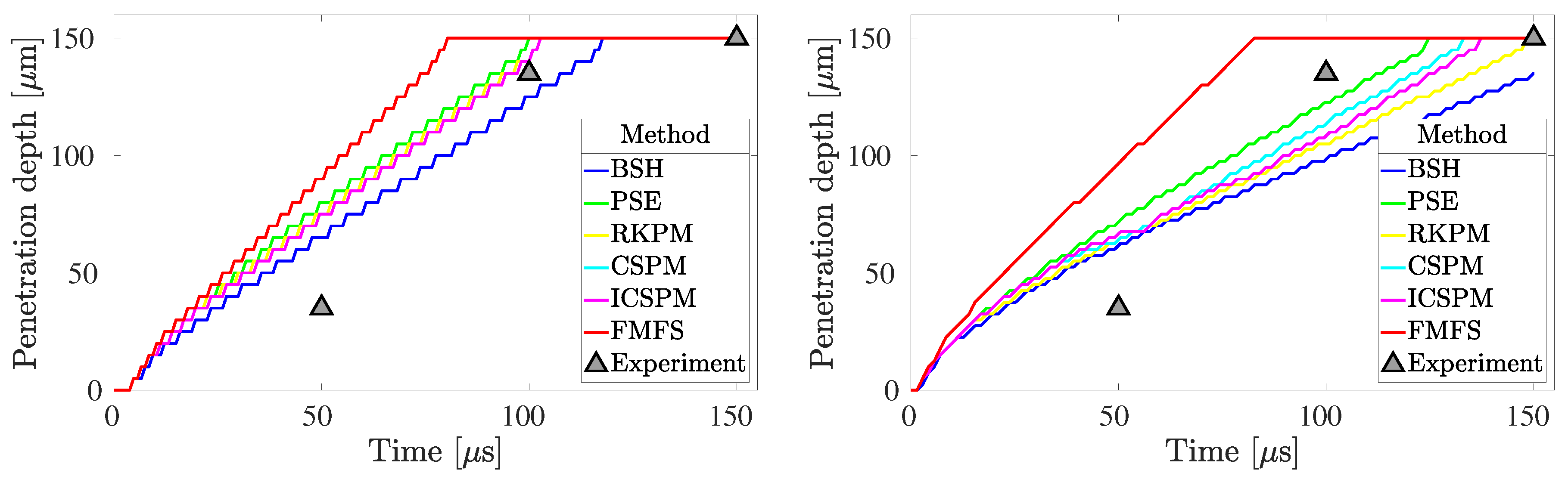
Due to the sufficient simplifications considered in this test model, any validation or comparison versus experimental measurements would be questionable at best. Nevertheless, it was still worthwhile to include a demonstration of the present result against other references. Simulated penetration depths computed by this code are plotted in Figure 7 for all six methods at two different resolutions. The numerical values and overall trend were found acceptable compared to the experimental data provided by [10] and the numerical solutions of [13]. It is important to mention that the numerical simulation presented by [13] was also performed by taking a set of assumptions similar to what was outlined in this paper.
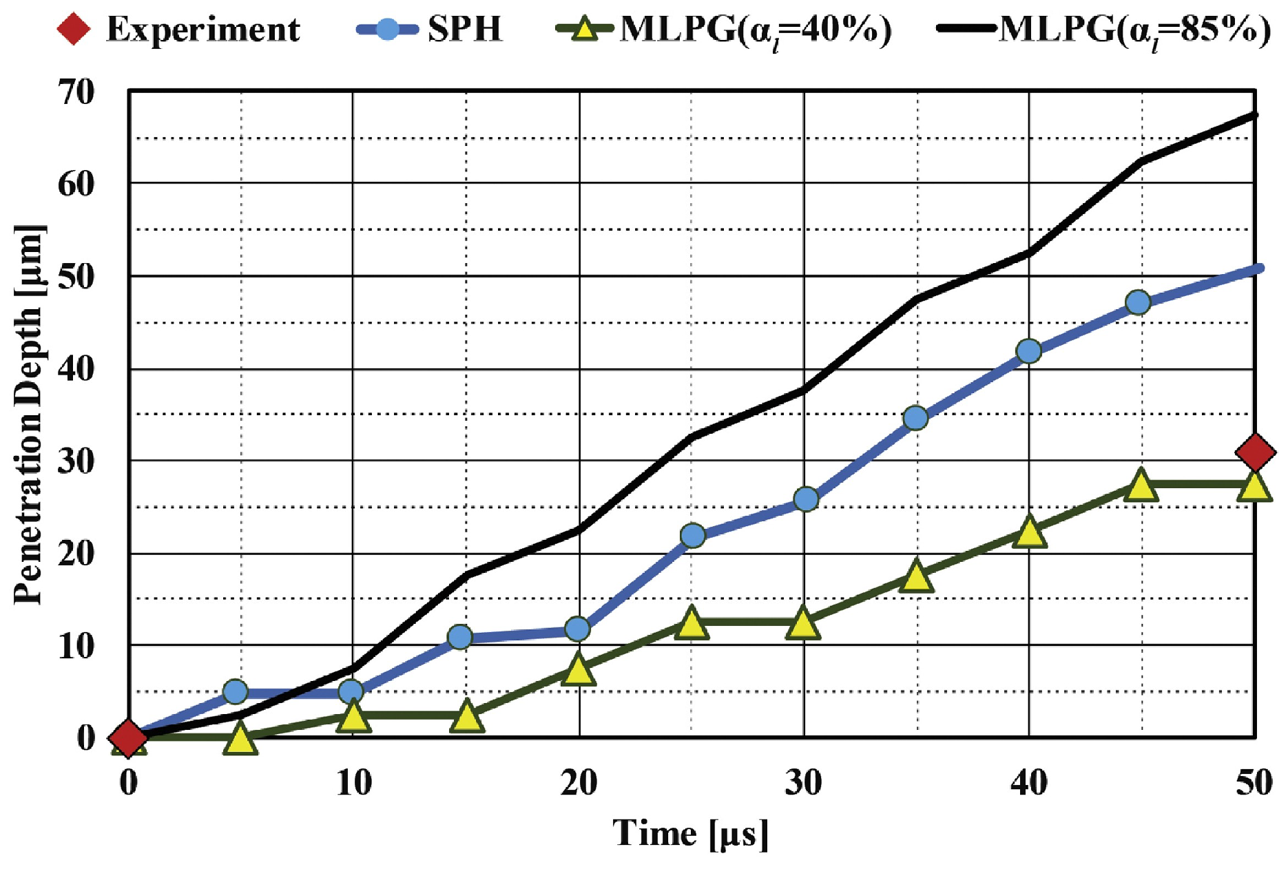
The experimental data points in Figure 8 were the penetration depth recorded for each pulse duration. In this figure, the presented methods were alternatively used to predict the penetration in time. A more or less linear behavior was noticed in all numerical graphs. According to the experimental evidence, however, the laser absorptivity coefficient at lower temperatures was less than its values at higher temperatures [10,12,13]. In other words, at the beginning of the laser drilling process, this coefficient had a lower value compared to the later stages, when it abruptly increased due to the rapid increase in both temperature and depth. Another reason for this behavior was that the laser beam was also defocused in lower parts of the hole, which indicated lower intensity and, therefore, lower heat input and surface temperature. In fact, the penetration speed was slow in the beginning as no multiple reflections occurred, and the laser due to the orthogonal irradiation had a low absorptivity. The speed increased due to multiple reflections and much better absorptivity on the steep walls. These were all the effects that were ignored by the simplifying assumptions in this paper and must be taken into consideration for future development.
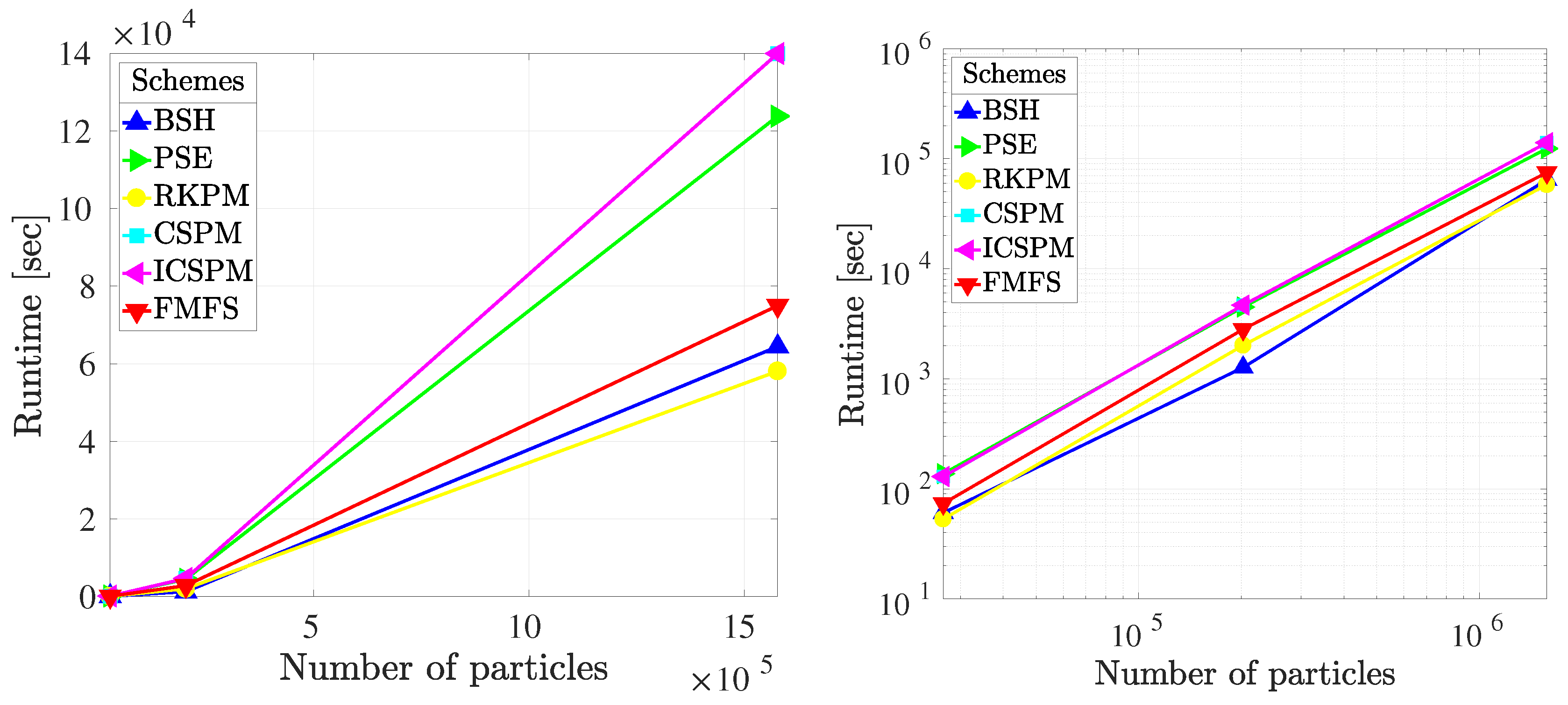
Next, we compared the computational performance of the presented methods by reporting their runtime at three different resolutions of 27 k, 203 k, and 1 . 6 mtotal particles. Both linear and log–log graphs are plotted in 
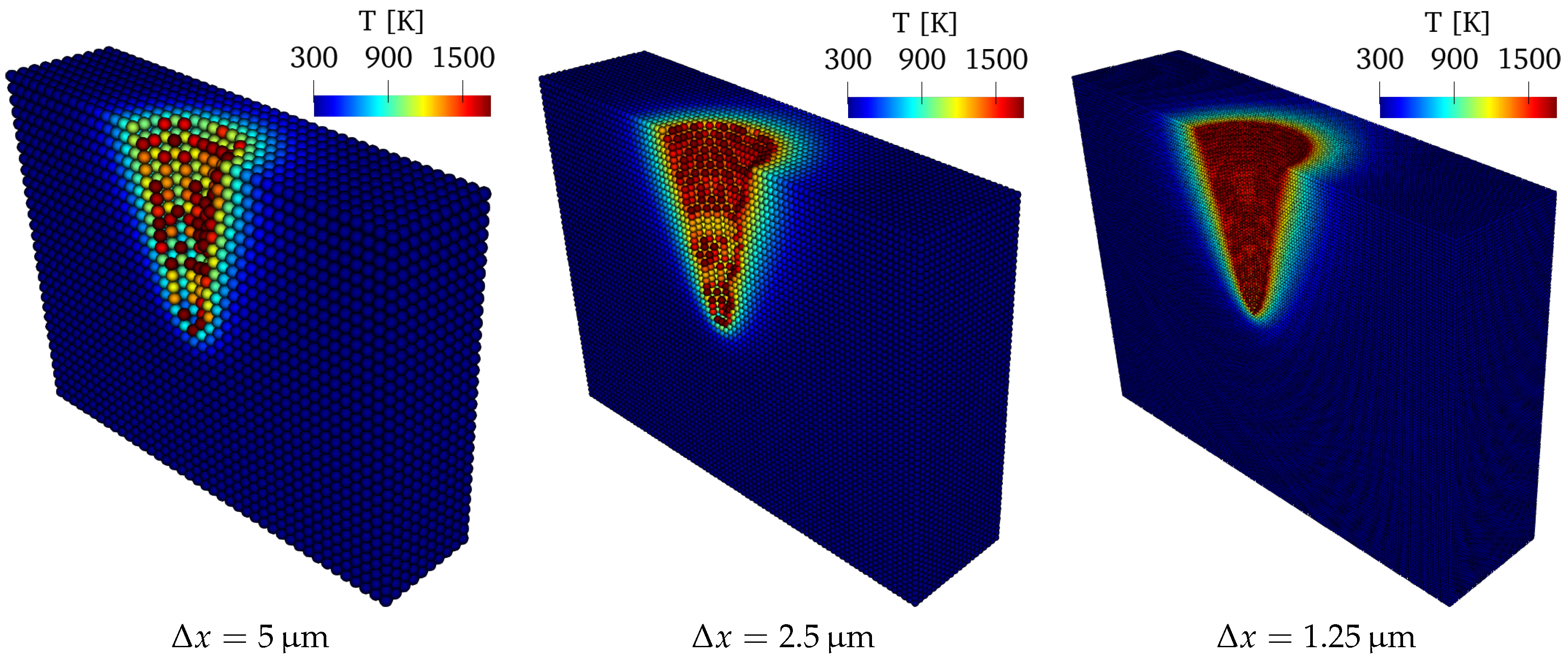
Figure 9, demonstrating the highest cost of computation for CSPM/ICSPM and the lowest for BSH. Furthermore, an exemplary snapshot of each resolution is represented in Figure 10 to illustrate the impact of (spatial) discretization size on the quality of the results.
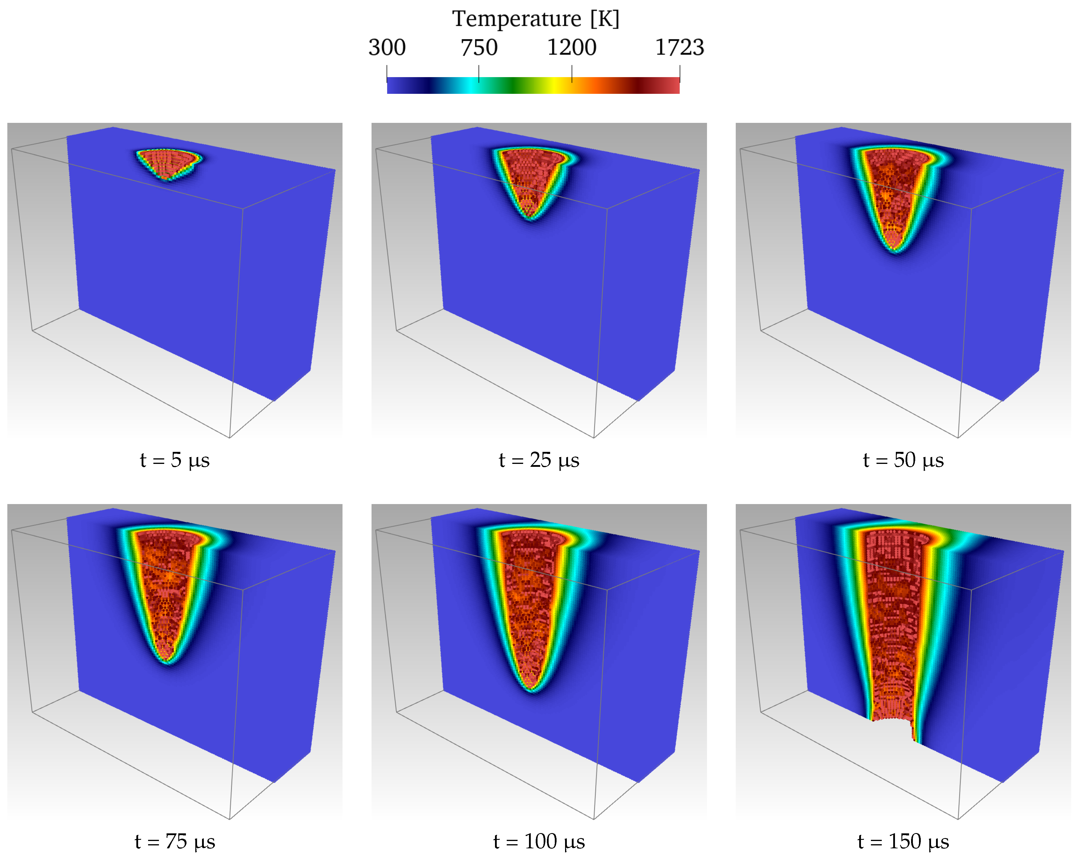
Lastly, images of the temperature distribution are provided in high resolution to gain more insights into the process. Figure 11 contains six frames of the simulation taken at six consecutive time instants, where PSE was employed for the discretization of the Laplacian operator. As a verification that our results were correct, the pictures in Figure 11 could be compared with those generated by [10,
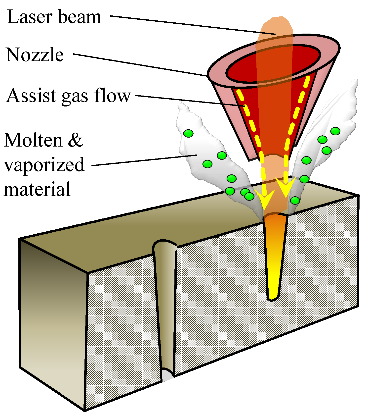
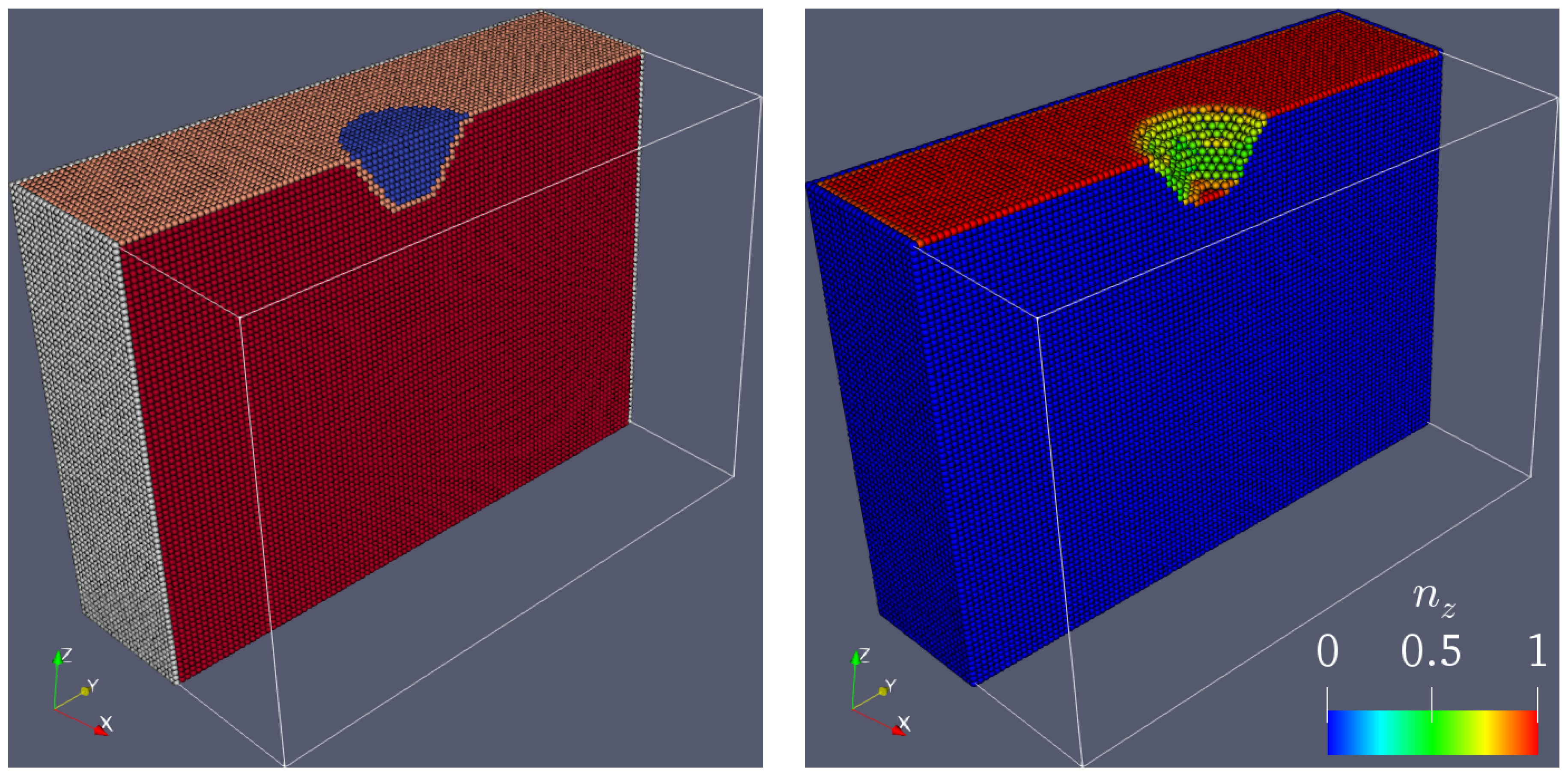
13] for a very similar case. These snapshots also served to represent how the laser-induced heat was transferred into the metallic workpiece, leading to the formation of the drilled hole. A summary of this scenario, which was captured by the present implementation rather nicely, follows. Initially, top surface particles absorbed the thermal energy provided by the laser beam. Due to the heat conduction, material particles were heated up until they reached the melting point and consequently become inactive in the simulation. These molten particles (invisible in Figure 11 because they were inactive in the model) were removed from the popped hole, and the laser beam was applied onto a newly generated surface (i.e., the orange particles in Figure 2). Therefore, the evolutionary boundary conditions during this procedure were effectively handled; the drilled hole was progressively developed; and the drilling penetration was obtained.

5. Conclusions

This paper developed a 3D numerical simulation framework that could return quantitative and qualitative insights into the thermal modeling of laser drilling processes. Six meshfree schemes with different orders of consistency were first cross-compared in a convergence study and then applied for the first time to the 3D thermal modeling of a laser drilling problem. While these methods shared some similarities in the quadratic rate of convergence for the approximation of the Laplace operator (see Figure 4), their computational cost and stability were fundamentally different in the laser drilling simulation (see Table 3, Table 4, Table 5 and Table 6 and Figure 9, for example). It was shown in Figure 6 that the total removed volume calculations compared well with those reported by [13] using the MPLG collocation method. Furthermore, the comparison of available experimental data from [10] and the penetration depth computed by this solver were found to be within an acceptable range considering the simplified modeling procedure. Nonetheless, model refinements and further experimental studies are envisaged to be necessary for better evaluation.
Overall, the computer code performed efficiently, and the implemented methods could provide useful insights into the thermal field and fundamental nature of a laser drilling process. However, an immediate enhancement to this work would adopt a more sophisticated approach for handling general boundary conditions where particles can freely move. Moreover, it is of utmost importance to include more physical phenomena in the description to increase the degree of realism required for a more realistic model. For instance, accounting for the change of laser absorptivity, modeling of the phase change, latent heat, the Marangoni effect, assist gas, molten particles, and recoil pressure could be added to future developments.

Author Contributions

M.A.: conceptualization, methodology, software, validation, formal analysis, investigation, resources, data curation, visualization, writing, original draft preparation, and writing, review and editing. K.W.: supervision, revision, project administration, and funding acquisition. All authors read and agreed to the published version of the manuscript.

Funding

This research was partially funded by the Swiss National Science Foundation Grant Number 200021-149436.

Acknowledgments

The authors sincerely thank Eleni Chatzi and Konstantinos Agathos for their support and constructive suggestions. M.A. is also grateful to Jeff Eldredge for enlightening about the 3D derivation of PSE kernels along with his instructive notes and to Matthias Roethlin for his integral contribution to this research project.

Conflicts of Interest

The authors declare no conflict of interest. The funders had no role in the design of the study; in the collection, analyses, or interpretation of data; in the writing of the manuscript; nor in the decision to publish the results.

Abbreviations

The following abbreviations are used in this manuscript:
CFDComputational Fluid Dynamics
CSPMCorrective Smoothed Particle Method
FDMFinite Difference Method
FEMFinite Element Method
FMFSFatehi’s Meshfree Scheme
FVMFinite Volume Method
ICSPMImproved CSPM
IPIMIsoparametric Point Interpolation Method
MLPGMeshless Local Petrov–Galerkin
PDEPartial Differential Equation
PSEParticle Strength Exchange
ODEOrdinary Differential Equation
RBFRadial Basis Function
RKPMReproducing Kernel Particle Method
RPIMRadial Point Interpolation Method
SPHSmoothed Particle Hydrodynamics

References

  1. Kim, M.; Majumdar, P. Computational model for high-energy laser-cutting process. Numer. Heat Transf. Part Appl. 1995, 27, 717–733. [Google Scholar] [CrossRef]
  2. Bamforth, P.; Williams, K.; Jackson, M. Edge quality optimisation for CO2 laser cutting of nylon textiles. Appl. Therm. Eng. 2006, 26, 403–412. [Google Scholar] [CrossRef]
  3. Ji, Z.; Wu, S. FEM simulation of the temperature field during the laser forming of sheet metal. J. Mater. Process. Technol. 1998, 74, 89–95. [Google Scholar] [CrossRef]
  4. Tsirkas, S.; Papanikos, P.; Kermanidis, T. Numerical simulation of the laser welding process in butt-joint specimens. J. Mater. Process. Technol. 2003, 134, 59–69. [Google Scholar] [CrossRef]
  5. Shalahim, N.; Mon, T.; Ismail, M.; Rashid, M.; Rejab, M. Finite element simulation of laser-micromachining. In Proceedings of the World Congress on Engineering, London, UK, 4–6 July 2012. [Google Scholar]
  6. Begic, D.; Bijelonja, I.; Kulenovic, M.; Cekic, A. Transient Evaporative Laser Cutting with Finite Volume Method. Available online: https://go.gale.com/ps/anonymous?id=GALE%7CA225316009&sid=googleScholar&v=2.1&it=r&linkaccess=abs&issn=17269679&p=AONE&sw=w (accessed on 13 May 2020).
  7. Gross, M. Smooth particle hydrodynamics (SPH) modelling of laser cutting. In International Congress on Applications of Lasers & Electro-Optics; Laser Institute of America: Orlando, FL, USA, 2008; Volume 2008, p. 1505. [Google Scholar]
  8. Demuth, C.; Bieda, M.; Lasagni, A.F.; Mahrle, A.; Wetzig, A.; Beyer, E. Thermal simulation of pulsed direct laser interference patterning of metallic substrates using the smoothed particle hydrodynamics approach. J. Mater. Process. Technol. 2012, 212, 689–699. [Google Scholar] [CrossRef]
  9. Kim, M.J. Meshfree isoparametric finite point interpolation method (IFPIM) with weak and strong forms for evaporative laser drilling. Appl. Math. Model. 2012, 36, 1615–1625. [Google Scholar] [CrossRef] [Green Version]
  10. Muhammad, N.; Rogers, B.; Li, L. Understanding the behaviour of pulsed laser dry and wet micromachining processes by multi-phase smoothed particle hydrodynamics (SPH) modelling. J. Phys. D Appl. Phys. 2013, 46, 095101. [Google Scholar] [CrossRef]
  11. Alshaer, A.; Rogers, B.; Li, L. Smoothed Particle Hydrodynamics (SPH) modelling of transient heat transfer in pulsed laser ablation of Al and associated free-surface problems. Comput. Mater. Sci. 2017, 127, 161–179. [Google Scholar] [CrossRef]
  12. Abidou, D.; Yusoff, N.; Nazri, N.; Awang, M.O.; Hassan, M.A.; Sarhan, A.A. Numerical simulation of metal removal in laser drilling using radial point interpolation method. Eng. Anal. Bound. Elem. 2017, 77, 89–96. [Google Scholar] [CrossRef]
  13. Abidou, D.; Sarhan, A.A.; Yusoff, N.; Nazri, N.; Awang, M.O.; Hassan, M.A. Numerical Simulation of Metal Removal in Laser Drilling using Meshless Local Petrov-Galerkin Collocation Method. Appl. Math. Model. 2018, 56, 239–253. [Google Scholar] [CrossRef]
  14. Afrasiabi, M.; Chatzi, E.; Wegener, K. A Particle Strength Exchange Method for Metal Removal in Laser Drilling. Procedia CIRP 2018, 72, 1548–1553. [Google Scholar] [CrossRef]
  15. Rabczuk, T.; Belytschko, T. A three-dimensional large deformation meshfree method for arbitrary evolving cracks. Comput. Methods Appl. Mech. Eng. 2007, 196, 2777–2799. [Google Scholar] [CrossRef] [Green Version]
  16. Adami, S.; Hu, X.; Adams, N. A new surface-tension formulation for multi-phase SPH using a reproducing divergence approximation. J. Comput. Phys. 2010, 229, 5011–5021. [Google Scholar] [CrossRef]
  17. Afrasiabi, M.; Roethlin, M.; Chatzi, E.; Wegener, K. A Robust Particle-Based Solver for Modeling Heat Transfer in Multiphase Flows. In Proceedings of the 6th European Conference on Computational Mechanics (ECCM 2018), Glasgow, UK, 11–15 June 2018. [Google Scholar]
  18. Limido, J.; Espinosa, C.; Salaün, M.; Lacome, J.L. SPH method applied to high speed cutting modelling. Int. J. Mech. Sci. 2007, 49, 898–908. [Google Scholar] [CrossRef] [Green Version]
  19. Afrasiabi, M.; Roethlin, M.; Klippel, H.; Wegener, K. Meshfree simulation of metal cutting: An updated Lagrangian approach with dynamic refinement. Int. J. Mech. Sci. 2019, 160, 451–466. [Google Scholar] [CrossRef]
  20. Roethlin, M.; Klippel, H.; Afrasiabi, M.; Wegener, K. Meshless single grain cutting simulations on the GPU. Int. J. Mechatronics Manuf. Syst. 2019, 12, 272–297. [Google Scholar] [CrossRef]
  21. Afrasiabi, M.; Meier, L.; Klippel, H.; Wegener, K. GPU-Accelerated Meshfree Simulations for Parameter Identification of a Friction Model in Metal Machining. Int. J. Mech. Sci. 2020, 176, 105571. [Google Scholar] [CrossRef]
  22. Brookshaw, L. A method of calculating radiative heat diffusion in particle simulations. Publ. Astron. Soc. Aust. 1985, 6, 207–210. [Google Scholar] [CrossRef]
  23. Mas-Gallic, S.; Raviart, P. Particle Approximation of Convection-Diffusion Problems; Technical Report R86013; Pierre and Marie Curie University Digital Analysis Laboratory: Paris, France, 1986; Volume 6. [Google Scholar]
  24. Liu, W.K.; Jun, S.; Zhang, Y.F. Reproducing kernel particle methods. Int. J. Numer. Methods Fluids 1995, 20, 1081–1106. [Google Scholar] [CrossRef]
  25. Chen, J.; Beraun, J.; Carney, T. A corrective smoothed particle method for boundary value problems in heat conduction. Int. J. Numer. Methods Eng. 1999, 46, 231–252. [Google Scholar] [CrossRef]
  26. Fatehi, R.; Manzari, M. Error estimation in smoothed particle hydrodynamics and a new scheme for second derivatives. Comput. Math. Appl. 2011, 61, 482–498. [Google Scholar] [CrossRef]
  27. Korzilius, S.; Schilders, W.; Anthonissen, M. An Improved CSPM Approach for Accurate Second-Derivative Approximations with SPH. J. Appl. Math. Phys. 2016, 5, 168. [Google Scholar] [CrossRef] [Green Version]
  28. Ng, G.; Crouse, P.; Li, L. An analytical model for laser drilling incorporating effects of exothermic reaction, pulse width and hole geometry. Int. J. Heat Mass Transf. 2006, 49, 1358–1374. [Google Scholar] [CrossRef]
  29. Monaghan, J.J. Smoothed particle hydrodynamics. Rep. Prog. Phys. 2005, 68, 1703. [Google Scholar] [CrossRef]
  30. Lucy, L.B. A numerical approach to the testing of the fission hypothesis. Astron. J. 1977, 82, 1013–1024. [Google Scholar] [CrossRef]
  31. Gingold, R.A.; Monaghan, J.J. Smoothed particle hydrodynamics: Theory and application to non-spherical stars. Mon. Not. R. Astron. Soc. 1977, 181, 375–389. [Google Scholar] [CrossRef]
  32. Li, S.; Liu, W.K. Meshfree and particle methods and their applications. Appl. Mech. Rev. 2002, 55, 1–34. [Google Scholar] [CrossRef]
  33. Choquin, J.; Huberson, S. Particles simulation of viscous flow. Comput. Fluids 1989, 17, 397–410. [Google Scholar] [CrossRef]
  34. Eldredge, J.D.; Leonard, A.; Colonius, T. A general deterministic treatment of derivatives in particle methods. J. Comput. Phys. 2002, 180, 686–709. [Google Scholar] [CrossRef] [Green Version]
  35. Afrasiabi, M.; Roethlin, M.; Wegener, K. Contemporary Meshfree Methods for Three Dimensional Heat Conduction Problems. Arch. Comput. Methods Eng. 2019, 1–35. [Google Scholar] [CrossRef]
  36. Chen, J.; Beraun, J. A generalized smoothed particle hydrodynamics method for nonlinear dynamic problems. Comput. Methods Appl. Mech. Eng. 2000, 190, 225–239. [Google Scholar] [CrossRef]
  37. Chen, J.; Beraun, J.; Jih, C. Completeness of corrective smoothed particle method for linear elastodynamics. Comput. Mech. 1999, 24, 273–285. [Google Scholar] [CrossRef]
  38. Afrasiabi, M.; Roethlin, M.; Wegener, K. Thermal simulation in multiphase incompressible flows using coupled meshfree and particle level set methods. Comput. Methods Appl. Mech. Eng. 2018, 336, 667–694. [Google Scholar] [CrossRef]
  39. Ahrens, J.; Geveci, B.; Law, C. Paraview: An end-user tool for large data visualization. Vis. Handb. 2005, 717, 1–17. [Google Scholar]
  40. Liu, G.R.; Liu, M.B. Smoothed Particle Hydrodynamics: A Meshfree Particle Method; World Scientific: Singapore, 2003. [Google Scholar]
  41. Liu, M.; Liu, G. Smoothed particle hydrodynamics (SPH): An overview and recent developments. Arch. Comput. Methods Eng. 2010, 17, 25–76. [Google Scholar] [CrossRef] [Green Version]
Figure 1. Schematic of a laser drilling process.
Jmmp 04 00058 g001
Figure 2. Illustration of how the proposed boundary treatment works. Left: the particle label is color coded, where red shows the active particles, white the wall boundaries, orange the laser surface, and blue the molten particles. Boundary conditions are applied to white and orange particles, while blue molten particles are effectively deleted from the simulation. Right: the color indicates the z-component of the unit normal vector pointing outward from the laser-irradiated surface, i.e., n z computed from Equation (22). The laser heat source expressed in Equation (2) is multiplied by n z for those particles exposed to the beam.
Jmmp 04 00058 g002
Figure 3. Uniform vs. random configuration of particles. Only a quarter of the cubic domain is clipped and shown for better visibility.
Jmmp 04 00058 g003
Figure 4. Convergence plots of the particle methods in a 3D heat conduction test. Left: regular spacing. Right: random spacing. The cubic B-spline kernel with h = 1.5 Δ x is used.
Jmmp 04 00058 g004
Figure 5. Experimental images of the penetration depth in a single-pulsed laser drilling test from [10]. Reprinted from [13], Copyright (2020), with permission from Elsevier under License Number 4835890957650.
Jmmp 04 00058 g005
Figure 6. Bar-chart comparison of the removed volume in the present 3D models versus the 2D reference solution of [13]. The label N p indicates the total number of particles.
Jmmp 04 00058 g006
Figure 7. Penetration depth of the laser in time, computed with a total of 27k (left) and 203k (right) particles. Experimental data points in these plots were read from [10].
Jmmp 04 00058 g007
Figure 8. Graph given by [13] demonstrating the numerically calculated penetration depth against experimental data points [10] where α l in this plot indicates the absorption coefficient. Reprinted from [13], Copyright (2020), with permission from Elsevier under License Number 4835890957650.
Jmmp 04 00058 g008
Figure 9. Comparison of the measured CPU times in both linear (left) and log–log (right) graphs.
Jmmp 04 00058 g009
Figure 10. Impact of the discretization size. Only half of the domain is shown for better visualization.
Jmmp 04 00058 g010
Figure 11. Formation of the popped hole due to heat transfer in a simplified laser drilling process. Snapshots of the temperature distribution were taken from a thermal simulation using PSE at a high resolution. The whole workpiece is discretized with approximately 672k particles, but only one half is shown for better visualization.
Jmmp 04 00058 g011
Table 1. Summary of the methods implemented in this work.
SchemeAcronymOrder of ConsistencyYearPublication
BrookSHaw’s approximationBSH1985[22]
Particle Strength ExchangePSE1986[23]
Reproducing Kernel Particle MethodRKPM1st1995[24]
Corrective Smoothed Particle MethodCSPM1st1999[25]
Fatehi’s Meshfree SchemeFMFS2nd2011[26]
Improved CSPMICSPM2nd2017[27]
Table 2. Parameters and material properties used according to [10,13].
PropertyUnitValue
Densitykg m 3 7950
Specific heat capacityJ kg 1 K 1 470
Heat conductivityW m 1 K 1 20
Heat convection coefficientW m 2 K 1 20
Stefan–Boltzmann constantW m 2 K 4 5.67×10 8
Emissivity factor0.4
Initial temperatureK300
Melting temperatureK1723
Laser powerW100
Laser absorptivity0.4
Laser beam radius μ m25
Table 3. Batch 1: Coarse discretization using a total of 27k particles with the cubic B-spline kernel.
MethodData h = Δ x h = 1 . 25 Δ x h = 1 . 5 Δ x
BSHRem.vol.(%)63.4174.3679.37
Full pen.
Runtime (s)3260102
PSERem. vol (%)72.8378.1383.4
Full pen.
Runtime (s)77137237
RKPMRem. vol. (%)63.2863.5378.18
Full pen.
Runtime (s)285386
CSPMRem. vol. (%)74.9983.82
Full pen.
Runtime (s)73130200
ICSPMRem. vol. (%)74.9983.02
Full pen.
Runtime (s)73131200
FMFSRem. vol. (%)80.7780.6884.76
Full pen.
Runtime (s)3874123
Table 4. Batch 2: Coarse discretization using a total of 27k particles with the Wendland quintic kernel.
MethodData h = Δ x h = 1 . 25 Δ x h = 1 . 5 Δ x
BSHRem. vol. (%)65.9572.6678.56
Full pen.
Runtime (s)3261101
PSERem. vol (%)72.8378.1383.4
Full pen.
Runtime (s)77137237
RKPMRem. vol. (%)78.4776.4480.47
Full pen.
Runtime (s)295388
CSPMRem. vol. (%)76.5277.6387.85
Full pen.
Runtime (s)73129205
ICSPMRem. vol. (%)76.5277.6789.51
Full pen.
Runtime (s)73129205
FMFSRem. vol. (%)80.4781.4485.39
Full pen.
Runtime (s)3874122
Table 5. Batch 3: Fine discretization using a total of 203k particles with the cubic B-spline kernel.
MethodData h = Δ x h = 1 . 25 Δ x h = 1 . 5 Δ x
BSHRem. vol. (%)40.1739.3568.66
Full pen.
Runtime (s)67112342095
PSERem. vol (%)60.2174.9286.73
Full pen.
Runtime (s)240544897628
RKPMRem. vol. (%)32.6133.42
Full pen.
Runtime (s)113421673536
CSPMRem. vol. (%)71.50
Full pen.
Runtime (s)258945415357
ICSPMRem. vol. (%)71.50
Full pen.
Runtime (s)259245155609
FMFSRem. vol. (%)87.7489.6390.69
Full pen.
Runtime (s)135826534433
Table 6. Batch 4: Fine discretization using a total of 203k particles with the Wendland quintic kernel.
MethodData h = Δ x h = 1 . 25 Δ x h = 1 . 5 Δ x
BSHRem. vol. (%)41.4839.0863.13
Full pen.
Runtime (s)66012682115
PSERem. vol (%)60.2174.9286.73
Full pen.
Runtime (s)240544897628
RKPMRem. vol. (%)87.0346.6948.91
Full pen.
Runtime (s)110620153364
CSPMRem. vol. (%)76.5169.0197.55
Full pen.
Runtime (s)202246667630
ICSPMRem. vol. (%)76.5163.43
Full pen.
Runtime (s)202846737591
FMFSRem. vol. (%)87.7489.4290.97
Full pen.
Runtime (s)121328194534

