An Analytic Approach to the Cox Proportional Hazards Model for Estimating the Lifespan of Cutting Tools

Abstract

The machining industry raises an ever-growing concern for the significant cost of cutting tools in the production process of mechanical parts, with a focus on the replacement policy of these inserts. While an early maintenance induces lower tool return on investment, scraps and inherent costs stem from late replacement. The framework of this paper is the attempt to predict the tool inserts Mean Up Time, based solely on the value of a cutting parameter (the cutting speed in this particular turning application). More specifically, the use of the Cox Proportional Hazards (PH) Model for this prediction is demonstrated. The main contribution of this paper is the analytic approach that was conducted about the relevance on data transformation prior to using the Cox PH Model. It is shown that the logarithm of the cutting speed is analytically much more relevant in the prediction of the Mean Up Time through the Cox PH model than the raw cutting speed value. The paper also covers a numerical validation designed to show and discuss the benefits of this data transformation and the overall interest of the Cox PH model for the lifetime prognosis. This methodology, however, necessitates the knowledge of an analytical law linking the covariate to the Mean Up Time. It also shows how the necessary data for the numerical experiment was obtained through a gamma process simulating the degradation of cutting inserts. The results of this paper are expected to help manufacturers in the assessment of tool lifespan.

1. Introduction

Little information is available to machining industry about proper cutting tools management. In most industrial cases, the decision of replacing a cutting insert is made entirely by the machining operator, and based on experience only. Meanwhile, an important fraction of the machining costs is linked with the tool maintenance itself [1,2,3], and in particular with improper management and poor maintenance decisions. A special aspect of this concern is the replacement policy of these inserts: while an early maintenance induces lower tool return on investment, scraps and inherent costs stem from late replacement [4]. In this last case, the important cost is due to dimensional discrepancies and bad surface finish of parts that are machined by worn tools. While standardized geometrical wear criteria for cutting inserts exist, their real-time quantification is not easily performed because said criteria cannot be measured while the machining operation is ongoing. Therefore, the general framework of this paper is the effort to provide aid for real-time quantification of the Remaining Useful Life (RUL) of a cutting insert.

While the wear phenomenon occurs in all machining operations, the present work is focused on turning. Among the types of wear, the present study considers the average flank wear, which is the nominal type of wear for the longest tool lifetime according to manufacturers of carbide inserts [5]. They consider that other forms of wear usually stem from poor cutting parameters choices [5]. However, this type of wear is also crucial, because of its important correlation with surface roughness, surface integrity and dimensional accuracy of the machined part.

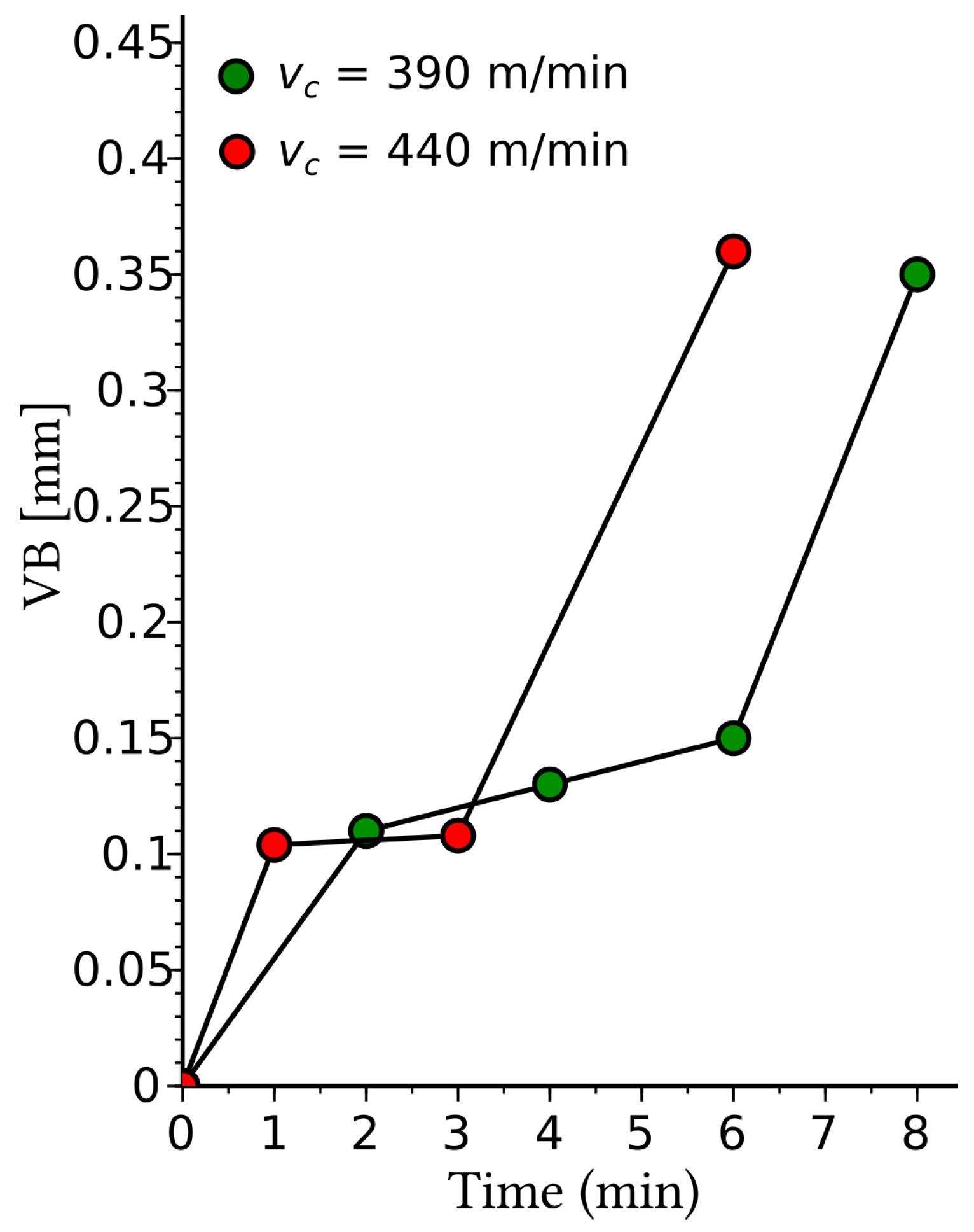
Flank wear is usually considered a result of abrasive wear, and it is influenced by the machining parameters, i.e., (in turning) cutting speed, depth of cut, and feed rate [6,7]. This degradation process is linked with abrasive wear, and incidentally with the hardness of machined materials. Regardless cutting parameters, the evolution of flank wear is usually divided into three phases: a first quick wear phase, followed by a longer steady-state region, and finally an accelerated wear after a given time. This evolution of the wear is always qualitatively similar albeit steeper as the cutting speed increases. The end-of-life criterion in life testing cases is given by the ISO 3685 standard as given in Equation (1) for average flank wear [8].

$$\mathrm{VB}=0.3\mathrm{mm}$$

(1)

Several works showed the interest of stochastic simulation of the evolution of degradation over time, using a stochastic model piloted by a gamma process modelling the monotonous characteristic of the process [9,10]. Letot et al. also demonstrated its use in this framework recently [11,12]. Numerous other models have been used in the specific approach of tool flank wear. Aramesh et al. showed the fit of the Weibull model to failure data of cutting tools [13]. Li also reviewed relevant mathematical models and numerical simulations [3]. Rizal et al. used a neuro-fuzzy inference system to extract specific characteristics from the force signal to predict the flank wear [14]. Moreover, they also showed a strong correlation between flank wear and feed force signals. Halila et al. [15] built a statistical model based on the Weibull model and proposed a new end-of-life criterion. More recently, machine learning techniques were also presented to determine the tool wear evolution. For example, training artificial neural networks and variants in order to determine the tool wear from tool micrography [16,17], or to predict the tool wear from condition monitoring variables such as cutting forces [18].

F. W. Taylor presented a relationship between the lifetime of a cutting tool (T) and the cutting speed ($v_c$) [19], which has been extensively discussed and used in numerous studies [6,7,11,20,21]. The Cox Proportional Hazards (PH) Model has been introduced by Cox in order to study the survival rates in medical context [22], but has since been widely used in mechanical engineering and in particular in maintenance and machining fields [23,24]. In earlier work, it has also been postulated that the influence of cutting parameters could therefore be used as the explanatory variable of a Cox PH Model, and experiments corroborated this postulate [12,13,25]. Furthermore, questions have been raised concerning the validity of data transformations when using the Cox PH Model [26].

A wide variety of wear indicators have also been associated with tool wear [27,28,29], therefore opening perspectives for online Tool Condition Monitoring [11,30]. Current approaches attempt to demonstrate the feasibility of prognosis regarding the Tool Lifetime based on few explanatory variables. In particular, previous studies showed the Tool Lifetime Prediction to lack accuracy at the borders of its learning interval [12]. The objective of this paper is to determine whether data transformation of the covariates may lead to improvement of the accuracy of the Cox PH Model precision. Through this objective, this paper aims specifically at improving the current approach using cutting parameters to estimate the Tool Lifetime via the Cox PH Model.

In this paper, the Cox PH Model itself is first described, and its choice and use in the case of cutting tools are explained. Second, the novelty of this contribution is developed, i.e., the analytic approach comparing the PH Model outputs with a theoretical law, and contribute to answer the issues raised by Feng et al. [26]. Later, the interest of this methodology is illustrated through a numerical validation, and the fitting methodology of the stochastic model that allows gathering of the necessary data for this experiment is shown. Finally, a general discussion of the approach shown in this work, and on perspectives concludes the paper.

2. Cox Proportional Hazards Model

Cox’s PH Model is the most important model in survival analysis [31]. It assumes the failure rate of a system to be a parametric function of a hazard baseline. The model relies on the assumption of the proportionality between the observed hazard rate and the baseline hazard function. The weighting of the respective influences of the covariates is usually expressed through an exponential function of a linear combination of the covariates.

The Cox PH Model has previously been shown to be well adapted to the evaluation of the Mean Up Time of mechanical equipment, and in particular of cutting inserts [13,25]. Aramesh et al. also stated that the Cox PH Model could take into account the ageing and cumulative wear of the tool, as well as cutting parameters and condition monitoring, which constitute the main advantages of the PH models in comparison with others [6].

In a general fashion, the Cox PH model can be expressed as follows:

$$h\left(t\right)=h_0\left(t\right)·exp\left(\sum _{i=1}^p{\beta }_i{\alpha }_i\right)$$

(2)

In this equation, $h\left(t\right)$ is the hazard function or failure rate, $h_0\left(t\right)$ is the baseline hazard function, ${\beta }_i$ the weighting coefficients for the p covariates and ${\alpha }_i$ the covariates.

In the framework of this paper, the only covariate that is taken into consideration is the cutting speed. The estimation of the only weighting coefficient $\beta$ and the baseline hazard curve are made through the computation of partial likelihood for $\beta$ and methods analogous to the Kaplan-Meier estimators for the baseline hazard curve $h_0\left(t\right)$, as Si et al. showed [23].

Because we chose to study the influence of only one covariate, Equation (2) can be simply written as:

$$h\left(t\right)=h_0\left(t\right)·exp\left(\beta v_c\right)$$

(3)

with $v_c$ the cutting speed. The Cox Model baseline can then be fitted to a Weibull distribution.

From the failure rate, which is fitted to a Weibull distribution, it is now possible to compute the reliability function. In a general case, the reliability of the cutting insert can be computed from the hazard baseline with help of Equation (4).

$$R\left(t\right)=exp\left(-{\int }_0^{+\infty }h\left(t\right)dt\right)$$

(4)

At this point, the distribution fitting provides us with the Weibull parameters, allowing the analytical obtaining of the reliability function as given in Equation (5):

$$R\left(t\right)=exp\left(-{\left(\frac{t}{\eta }\right)}^k\right)$$

(5)

In this equation, $R\left(t\right)$ is the reliability function in the case of a 2-parameter Weibull distribution, $\eta$ being the scale parameter and k the shape parameter of the Weibull distribution.

Therefore, the Mean Up Time (MUT) of the cutting inserts can be computed through Equation (6). It is to be considered to be a prediction for the cutting insert lifetime:

$$MUT={\int }_0^{+\infty }R\left(t\right)dt$$

(6)

This method for computing the Mean Up Time is classical and is used in a variety of similar works [4,6,12,13]. However, as previous work showed [12], while the quality of the prediction is very good within the learning interval, the quality of the prediction rapidly drops near the border of the learning interval, which impedes the use of this method for providing extrapolating prognosis. The mathematical interpretation of this behavior was found to be the inability of the usual approach using the Cox PH Model to reproduce the concavity of the observed experimental data [12].

3. Analytical Expression of the MUT and Data Transformation

In the case of estimating the MUT from cutting speeds, the Cox PH Model lifetime prediction, without data transformation, tends to be lower than the observed life duration at both ends of the learning set [12]. Therefore, we question the ability of the PH Model to replicate the curvature of the observed data curve in its prediction. Our inference is that analytical examination of the MUT as predicted by the PH Model is necessary to determine why the model deviates from the observed samples at the ends of the learning interval.

The MUT as computed in Equation (6) though the Cox PH Model is a result of computations performed on experimental data through Equation (3). It is, therefore, of major interest to ensure that the general expression of the Cox PH Model can reproduce the analytical influence of the covariate on the MUT. Taylor’s law provides such an analytical relationship linking the tool lifetime with the cutting speed [19]:

$$v_c{T}^n=C_T$$

(7)

With T the cutting tool lifetime (that we assimilate here to the MUT), n Taylor’s exponent and $C_T$ a constant that depends on the tool and the material being used. The objective of this analytic approach is to verify whether Equation (6) may be of the same form as Equation (7).

Mathematically stated:

$${\int }_0^{+\infty }{R}_{\mathrm{Cox}}\left(t\right)dt\stackrel{?}{=}{\left(\frac{C_T}{v_c}\right)}^{1/n}$$

(8)

This equation must be developed to achieve a clear answer, but two assumptions must be made at this point to obtain the analytic expressions that can be compared:

• the hazard baseline function is fitted on a Weibull distribution
• the Mean Up Time of the experimental sample that allowed to fit the Cox PH Model follows Equation (7)

Statistical reliability relationships define the following expression, where $f\left(t\right)$ is the failure probability density function:

$$h\left(t\right)=\frac{f\left(t\right)}{R\left(t\right)}=-\frac{\frac{dR\left(t\right)}{dt}}{R\left(t\right)}$$

(9)

therefore,

$$h\left(t\right)=-\frac{d}{dt}\left(log\left(R\right(t\left)\right)\right)$$

(10)

Because the failure rate is obtained through the Cox PHM, and fitted to a Weibull model, the left side of Equation (10) can be substituted with Equation (3), using the analytical expression of the failure rate in the case of a Weibull distribution:

$$\int \left(\frac{k}{\eta }\right){\left(\frac{t}{\eta }\right)}^{k-1}exp\left(\beta v_c\right)dt=-log\left(R\left(t\right)\right)$$

(11)

The initial conditions giving a unitary reliability, the integration constant is null and Equation (11) becomes:

$$R\left(t\right)=exp\left(-{\left(\frac{t}{\eta }\right)}^k·exp\left(\beta v_c\right)\right)$$

(12)

Therefore, the left-hand side of Equation (8) becomes:

$${\displaystyle {\int }_0^{+\infty }exp\left(-{\left(\frac{t}{\eta }\right)}^k·exp\left(\beta v_c\right)\right)dt\stackrel{?}{=}{\left(\frac{C_T}{v_c}\right)}^{1/n}}$$

(13)

The left-hand side can be integrated if ${\displaystyle \frac{exp\left(\beta v_c\right)}{{\eta }^k}>0}$ and $k>0$. Both conditions being always true, Equation (13) becomes:

$$\frac{\mathsf{\Gamma }(1/k)}{k{\left(\frac{exp\left(\beta v_c\right)}{{\eta }^k}\right)}^{1/k}}\stackrel{?}{=}{\left(\frac{C_T}{v_c}\right)}^{1/n}$$

(14)

The gamma function $\mathsf{\Gamma }\left(x\right)$ is defined as given in Equation (15) [32].

$$\mathsf{\Gamma }\left(x\right)={\int }_0^{+\infty }{t}^{x-1}exp(-t)dt$$

(15)

At this stage, the simplest strategy is to compare the sides of Equation (14), and to determine whether both sides have similar expressions of $v_c$.

For the constant part:

$$C_T={\left(\frac{\mathsf{\Gamma }(1/k)\eta }{k}\right)}^n$$

(16)

This equation can be true, and the fitting of the Weibull model to the survival baseline curve aims at verifying this equation. As for the $v_c$ part:

$$exp\left(\frac{\beta ·v_c}{k}\right)\ne v_c^{1/n}$$

(17)

Equation (17) is never verified. Therefore, it can be concluded that the Cox PH Model is intrinsically unable to produce a prognosis that follows Taylor’s law while using $v_c$ as covariate without data transformation.

However, the notation $v_c$ in the left-hand side of Equation (17) should be interpreted as the covariate used in the Cox PH Model. Instead, we can denote this input as any time-independent function of the cutting speed: $f\left(v_c\right)$, despite Cox’s original paper mainly pointing to a linear function [22,33]. Then, the objective becomes the search for a function $f\left(v_c\right)$ such that it would allow the last equation to be true, which becomes evident:

$$f\left(v_c\right)=\frac{klog\left(v_c\right)}{n\beta }$$

(18)

which is an adequate data transformation to allow proper results of the Cox PH Model. This function being time-independent, it will not affect the integration. The coefficients that appear in this final equation involve the Weibull distribution parameters. Their value would be absorbed by the weighting coefficient $\beta$ during the process of fitting the Cox PH Model. Thus, only nonlinear transformations should be taken into consideration at this stage.

This analytical approach therefore brings forward the necessity of performing a data transformation on the covariate $v_c$ before fitting the Cox PH Model and the subsequent Weibull distribution. The covariate that must be used in this fit is no longer $v_c$ but rather $log\left(v_c\right)$. This transformation should provide much more accurate results in fitting the PH Model. It can also be checked whether this transformation reduces the size of the sample that is necessary to achieve convergence of the PH Model. This question arises because the analytical approach modifies the Cox PH Model equation in a way that allows its MUT prediction to fit the analytical law that describes the phenomenon (in this case, Taylor’s law). This issue is assessed in the numerical validation.

Furthermore, similar approaches could be performed for any covariate describing the system. In actuality, only the first assumption (that the hazard baseline is fitted to a Weibull distribution) is strictly necessary for the reasoning to be true. Even in the case of this assumption not being verified, similar approaches could be pursued for other statistical distributions if necessary. Special caution must be paid while integrating Equation (13): some distributions may not provide with an expression that can be integrated. The second assumption is not necessary under the formulation that was given: any analytical law that describes the relationship between the covariate and the lifetime can be used. However, the right-hand side of Equation (13) must have a shape that is compatible with the comparison approach that was used on Equations (16) and (17).

The analytical developments using the logarithmic transformation lead from Equations (16) and (17) to respectively Equations (19) and (20), which can be analytically satisfied regardless the value of $v_c$, and in practice through the fitting of the PH Model and the Weibull model to the survival baseline curve.

$$C_T={\left(\frac{\mathsf{\Gamma }(1/k)\eta }{k}\right)}^{\frac{k}{\beta }}$$

(19)

$$n=\frac{k}{\beta }$$

(20)

This development therefore confirms that the raw cutting speed value cannot be a satisfactory Cox PH Model covariate, because regardless how good the model fitting may be, it cannot replicate the analytical link between the cutting speed and the tool life.

4. Materials and Methods

To assess the analytical development that was described in the previous section, it is intended to show an experimental validation based on tool life duration data obtained through a stochastic degradation process.

The research technique is based on the following process:

• Degradation paths based on a gamma process are generated. This gamma process is fitted on experimental tool wear evolution data.
• The degradation paths are used to generate a set of tool lifetimes (each curve yields a lifetime when it crosses the tool end-of-life threshold).
• These lifetimes are used to fit and assess the Cox PH model with and without the identified data transformation, to assess the benefits of the proposed methodology.

4.1. Piecewise Stochastic Flank Wear Model

In previous studies, several stochastic models of the degradation evolution using a gamma process were constructed [11,12,34]. The gamma process is widely considered in various research topics involving monotonous processes, such as reliability analyses and maintenance optimization of ageing systems [10]. Its monotonic behavior makes it particularly well suited for the modelling of physical degradation, i.e., wear, crack propagation, corrosion, etc. Therefore, the gamma process is particularly well adapted to represent the flank wear evolution of cutting tool inserts [35].

If $Z\left(t\right)$ denotes the evolution of the degradation process with respect to time, and $Z\left(t_0\right)$ is the initial degradation, then:

$$Z\left(t\right)=Z\left(t_0\right)+G\left(t\right|m\left(t\right),\lambda )$$

(21)

G is the gamma process, and has the following characteristics:

• G has independent increments;
• $G\left(0\right)=0$;
• G is a stochastic continuous process, and $\forall t_2,t_1(t_2\ge t_1\ge 0)$, the intensity of the jump $G\left(t_2\right)-G\left(t_1\right)$ follows a gamma distribution with shape parameter $m\left(t_2\right)-m\left(t_1\right)$ and scale parameter $\lambda$ with density function:

  $${\displaystyle f\left(x\right)=\frac{{\lambda }^{m\left(t_2\right)-m\left(t_1\right)}}{\mathsf{\Gamma }(m\left(t_2\right)-m\left(t_1\right))}{x}^{m\left(t_2\right)-m\left(t_1\right)-1}exp(-\lambda x)}$$

  (22)

A characteristic of the gamma function is its domain being ${\mathbb{R}}^{+}$, therefore producing only positive increments. The mathematical expectation and variance of the gamma process at any given time t are:

$$E\left(G\left(t\right|m\left(t\right),\lambda )\right)=\frac{m\left(t\right)}{\lambda }$$

(23)

$$V\left(G\left(t\right|m\left(t\right),\lambda )\right)=\frac{m\left(t\right)}{{\lambda }^2}$$

(24)

If the shape parameter is a linear function of time ($m\left(t\right)=\alpha t$), then the gamma process is stationary. The degradation process may be into time slices depending on the experimental inspection intervals. The interest and the fitting of this piecewise gamma process in comparison with nonlinear processes, especially in the case of the wear of cutting inserts, was already discussed [34]. This approach allows close replication of the non-stationary effects that occur at the beginning and the end of the tool life.

4.2. Gamma Process Fitting on Experimental Data

In this case, the data set used to create this model was obtained by gathering 29 replications of turning 322 Hv FGL250 cylinders with a diameter of 190 mm and a length of 220 mm on a CNC SOMAB “UNIMAB 450” lathe, using a cutting tool DCLNL 2525M 12 with CNMG 1204 085B OR SAFETY SA coated tungsten carbide inserts [11]. The depth of cut is kept constant at 1.5 mm and the feed at 0.18 mm/rev. The cutting speed is first kept constant at 340 m/min for the 29 degradation trajectories, then the experiment is repeated at different cutting speeds. The degradation evolution paths of the cutting inserts with machining time is represented in Figure 1 for the repetitions at constant cutting speed, and in Figure 2 at the other cutting speeds. In Figure 1, the time slicing relative to the piecewise approach are highlighted: the time intervals for which a gamma process is fitted are represented at the top of the figure, and the corresponding gamma parameters are computed in

Table 1. Parameters of the piecewise linear gamma process. Data from [34].

${\mathit{G}}_{\mathit{i}}({\mathit{\alpha }}_{\mathit{i}},{\mathit{\lambda }}_{\mathit{i}})$	${\mathit{G}}_1$	${\mathit{G}}_2$	${\mathit{G}}_3$	${\mathit{G}}_4$	${\mathit{G}}_5$	${\mathit{G}}_6$	${\mathit{G}}_7$	${\mathit{G}}_8$	${\mathit{G}}_9$	${\mathit{G}}_{10}$	${\mathit{G}}_{11+}$
${\alpha }_i$	$349.65$	$7.12$	$7.62$	$2.54$	$2.46$	$2.14$	$1.19$	$1.48$	$2.15$	$1.11$	$1.59$
${\lambda }_i$	$5583.64$	$580.07$	$378.36$	$291.01$	$307.40$	$382.25$	$91.27$	$138.41$	$210.99$	$12.46$	$8.49$

. The model fitting is performed through a maximum likelihood method [34].

.

The model is extended to various cutting speeds by using Taylor’s tool life equation [19]:

$$v_c{T}^n=C_T$$

(25)

Given experimental points for the lifetime of cutting inserts at different cutting speeds, the Taylor parameters n and $C_T$ can be found. In the case of this study, these values were found to be: $n=0.383$ and $C_T=840$. Taking advantage of the use of piecewise linear gamma process, simple lifetime corrections may be added through a modification of each of the shape parameters of the gamma processes. Indeed, the expected value of the gamma process is a linear image of the shape parameter [34]. Therefore, a correcting factor $T_{ref}/T_c$ can be introduced to the shape parameters, where $T_{ref}$ is the average tool lifetime at reference cutting speed $v_{c,ref}$ and $T_c$ is the computed tool duration at the considered cutting speed.

4.3. Numerical Validation

The general principle of this numerical experiment is to generate degradation trajectories based on the stochastic model of the tool wear degradation [12]. The time values at which each trajectory crosses the end-of-life degradation criterion provided in Equation (1) constitute our set of generated tool lifetimes.

Let us remember that the stochastic approach allows us to generate failure times for different cutting parameters. Two sets of 2000 trajectories of degradation each were generated for 20 different cutting speeds (100 trajectories per cutting speed value, the evenly distributed cutting speed values ranging from 280 to 470 m/min). The cutting speeds were chosen in order to discretize the interval of possible cutting speeds for this tool proposed by the manufacturer’s catalog, and 20 discrete values of cutting speeds are sufficient to highlight the interest of the data transformation, as shown in Section 5. 500 trajectories are sufficient to ensure convergence [36], but given the low computational cost, 2000 trajectories were generated. Furthermore, the convergence is also shown in Section 5. Of those two sets of 2000 trajectories, one was used for learning, and the other as control. The two sets were generated separately but following the same procedure, to ensure their statistical equivalence. A Cox PH Model was fitted on the learning set. The PH Model was used to produce predictions for evenly spread cutting speeds in the learning interval. These predictions were then compared to the control sample.

5. Results and Discussion

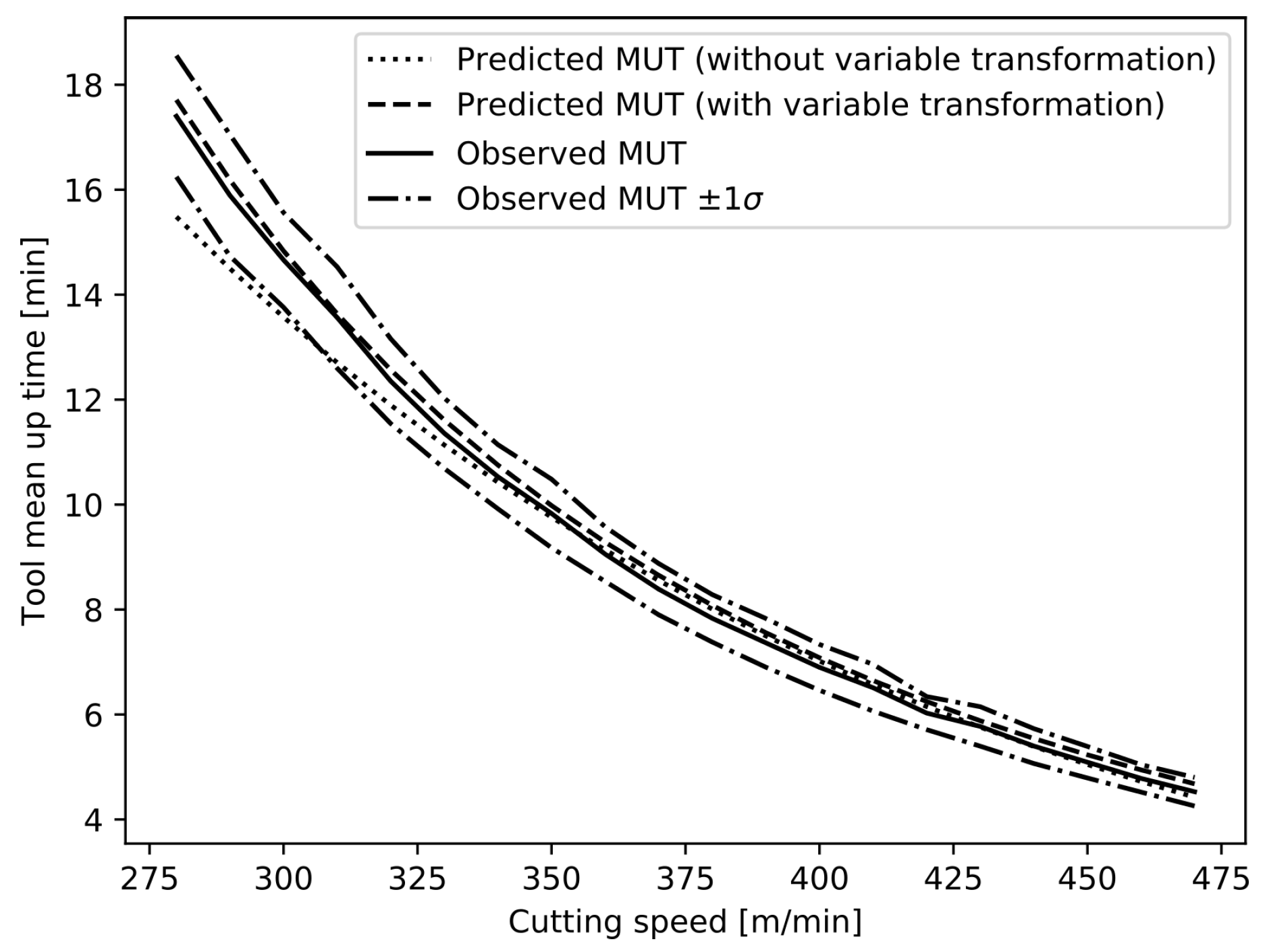
The numerical experiment was performed first without data transformation. In that case, the Cox PH Model received the cutting speed $v_c$ as a covariate. On the second experiment, the Cox PH Model received the natural logarithm of the cutting speed $log{v}_c$ as a covariate. In the first case, depicted dotted in Figure 3, as in previous studies, the prediction is shown to underestimate the actual lifetime of the cutting inserts, even within the learning range of the Cox PH Model, and especially for lower cutting speeds [12].

These results are to be compared with the dashed results presented in Figure 3. In particular, the left-hand part of the graph shows the correction for lower cutting speeds, and the predicted tool lifetimes better fit the curvature of the observed data, thanks to the data transformation. The model however diverges from the mean observed value. This effect can be attributed to the fitting method of the Cox Proportional Hazards Model (max partial-likelihood method), as opposed to the arithmetic mean that is shown on this Figure.

The comparison between both prediction curves in Figure 3 shows that without data transformation, the prediction is underestimated by more than one standard deviation at the lower border of the learning interval. In the case shown in Figure 3, this leads to an underestimation of the cutting tool lifespan by 11.1% at 280 m/min without data transformation, compared to an overestimation of 1.7% by the model with data transformation at the same cutting speed. This phenomenon is reduced with the data transformation; therefore, it supports the interest of the data transformation that was proposed.

To assess the capability of the Cox Model to match the Taylor parameters used to pilot the stochastic model that created its learning and control sets, they were estimated through a least square regression. The results of this regression are compared between the model constructed with and without data transformation in

Table 2. Least squares estimated values, coefficient, and relative error ($ϵ$) on the Taylor parameters from the MUT predictions with and without data transformation, compared to the learning set values.

	Without Data Transformation	With Data Transformation	Generated Data
n	0.412	0.389	0.384
$C_T$	885.5	856.7	839.7
$R^2$	0.995	1	-
$ϵ\left(n\right)$	7.8%	1.7%	-
$ϵ\left(C_T\right)$	6%	2.5%	-

.

This data transformation is therefore necessary for the Cox PH Model to produce a prediction that bears an analytical compatibility with correct replication of the analytical model (in this case, Taylor’s law). We showed that applying this procedure reduces the error of the prediction, and we can expect this error reduction to be of essential importance when using several covariates, in particular at the edge of the learning interval for each covariate. This is because the deviation observed on the prediction with one covariate would suffer from the combination of deviations due to each used covariate.

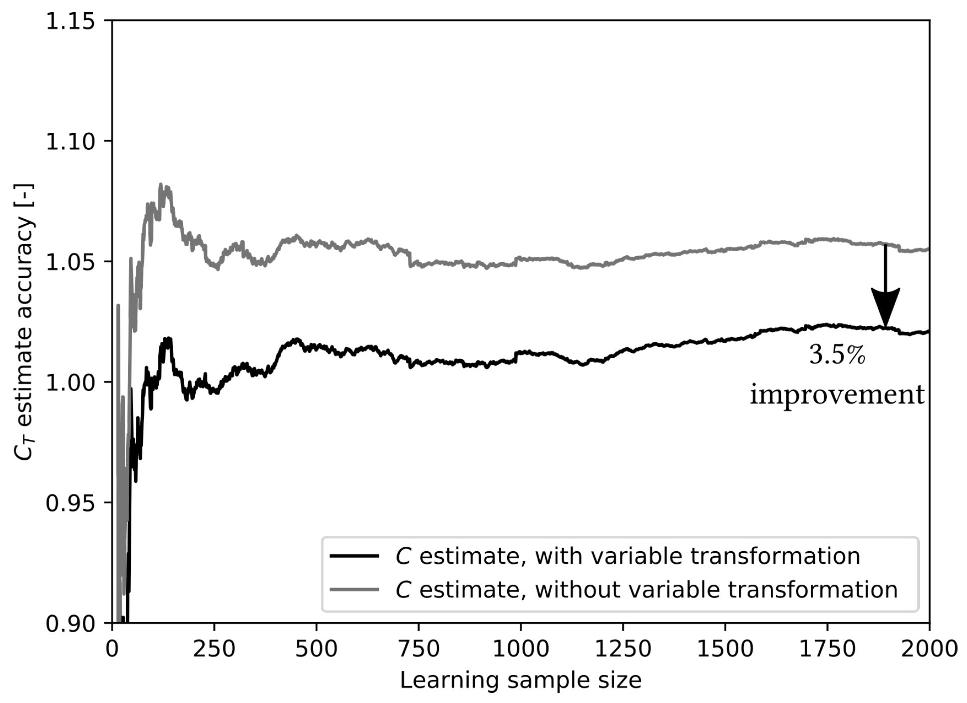
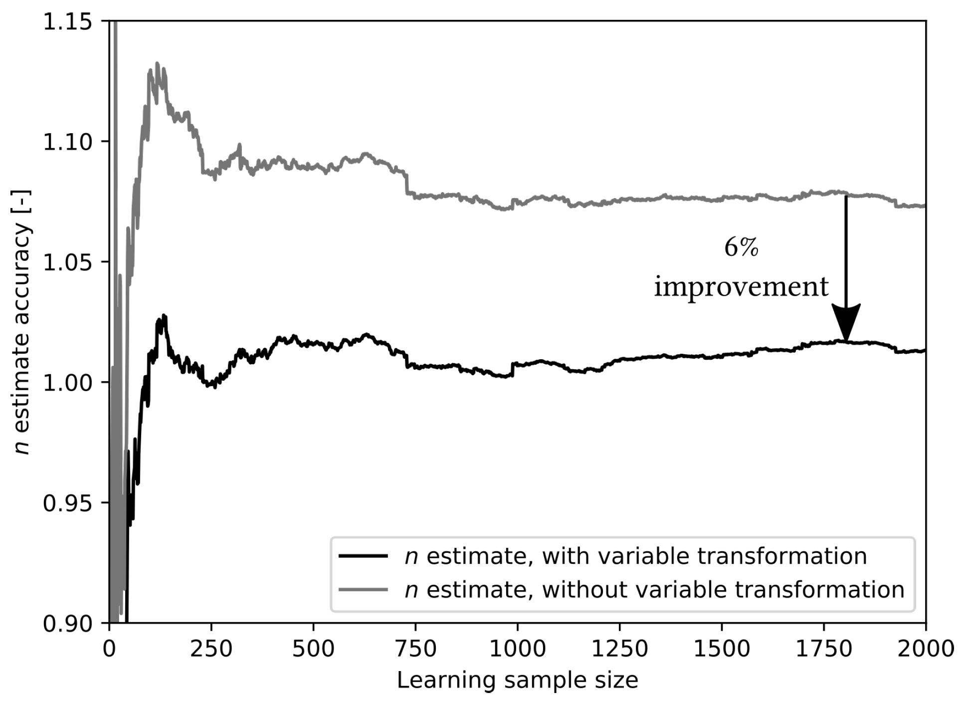
On the other hand, this methodology necessitates the previous knowledge of analytical laws linking the covariates with the MUT prediction (such as Taylor’s laws for cutting parameters), which will in turn allow performance of this analytical method and determine the correct data transformation that must be made for each used covariate. The better model performance due to the data transformation could also tend to suggest that smaller learning samples would be necessary to obtain a convergence. This assumption can be assessed: the Cox PH Model can be fitted to both log-transformed and non-transformed datasets of increasing learning sizes. Then, each time the model is fitted, the corresponding n and $C_T$ can be estimated and compared to the mean observed value of the complete sample.

This comparison is done for both Taylor parameters in Figure 4 and Figure 5. These figures represent the evolution accuracy of the parameters estimates (i.e., the ratio between the Cox-predicted value and the arithmetic average value over the total sample). They also allow to clearly see the convergence of the model results given the sample size. The offset in the estimate of both parameters is clear, regardless the sample size. The results show that an admissible value, within a relative error of 5%, is reached within a sample size of 25 (i.e., 25 data points are sufficient to reach the asymptotic value of the Taylor coefficients within a margin of ±5%). Furthermore, while a large offset separates the curves, it seems to remain similar in value throughout the sample size growth. Furthermore, the changes in predicted values follow the same tendency on both curves, linking them with the variability of generated data rather than inherent failure to converge from either model.

6. Conclusions

In this paper, issues raised in previous work were addressed [11,12,26]: the necessity of data transformation in using the Cox PH Model, and the nature of this transformation. A methodology used for creating a stochastic model relative to cutting tools in turning in cast iron was showed. The use of a Cox PH Model in survival analysis of cutting tools was discussed, and it was used to predict the Mean Up Time of tools.

More importantly, facing previous discrepancies and issues with data transformation and the Cox PH Model, the origins of discrepancies, that were brought forward by previous work, were highlighted. In the case of the cutting speed, a logarithmic data transformation has been proposed that was tested in the experimental part. Through a numerical validation, the data transformation has been shown to have positive qualitative and quantitative effects on the MUT prediction of the model. It was shown that few data is sufficient for an approximate estimate of the tool useful life through the Cox PH Model.

The analytical methodology that was demonstrated should be replicated on further studies using the Cox PH Model if an analytical model linking the covariate to the MUT exists. If further experiments confirm the interest of analogous analytical methodologies in mechanical framework or other uses of the Cox PH Model, the use of this approach should be generally recommended. On an industrial point of view, it is expected that the present methodology may contribute to a general condition monitoring framework, this emancipating from the control charts methodology that may prove conservative and constraining in some cases.