Abstract
This work presents a new methodology for machine tools anomaly detection via operational data processing. The previous methodology has been field tested on a milling-boring machine in a real production environment. This paper also describes the data acquisition process, as well as the technical architecture needed for data processing. Subsequently, a technique for operational machine data segmentation based on dynamic time warping and hierarchical clustering is introduced. The formerly mentioned data segmentation and analysis technique allows for machine tools anomaly detection thanks to comparison between near real-time machine operational information, coming from strategically positioned sensors and outcomes collected from previous production cycles. Anomaly detection techniques shown in this article could achieve significant production improvements: “zero-defect manufacturing”, boosting factory efficiency, production plans scrap minimization, improvement of product quality, and the enhancement of overall equipment productivity.
1. Introduction
Industry 4.0 is about the significant transformation taking place in the way goods are produced now [1]. The term Industry 4.0 (“Industrie 4.0” (I40)) was coined by the German government as one of 10 “Future Projects” part of its High-Tech Strategy 2020 Action Plan [2]. Industry 4.0 is being considered the fourth generation of industrial revolution and it is based on the so-called cyber-physical system (CPS) [3], which enables manufacturing and service innovation.
Smart production is based on process digitization and the competitive advantage given by the exploitation of the enormous sets of data obtained from a wide range of sources: from computer numeric control (CNC) machine tools, programmable logic controller (PLC), industrial control systems (ICS), supervisory control and data acquisition (SCADA), temperature sensors, and customer data, among others [4]. The previous sentence also introduced a very trendy concept nowadays, the internet of things (IoT) and the industrial internet concept. The later originated in the United States and partially overlaps the German concept of Industry 4.0 [5]. According to sources of the industry a 15% drop in unplanned downtime is gathered and a 7% increase in product quality is achieved after smart manufacturing is implemented, and the later facts are showing that when sensor data is captured and analyzed, between 2.3 and three times improvement in quality and productivity are attained [6]. Hence, significant gains await industries that strike out into digital transformation [7,8].
However, the transition to Industry 4.0 and smart manufacturing is not a straight forward road. It will be driven by the adoption of bleeding-edge information and communication technologies (ICT) and flexible solutions such as fast, reliable, and secure connectivity and high device density capable infrastructures [9]. Smart production is also about sharing information, collaborative manufacturing and machines talking to each other [10]. Perhaps, one of the most obvious cases on collaborative mechanization could be when a machine stops and tells the others in the production floor to stop too. Chances are, that if a machine is going to be sent a part, is no longer running properly, and there could be good reason for it to stop as well. Further to this, if greater intelligence is added, and machines are able to interact with other surrounding systems having direct impacts on their performance, we could ultimately achieve self-aware and self-learning machine tools. Thereupon, concepts such as Industry 4.0, smart manufacturing, anomaly detection, predictive maintenance, and ICT are closely intertwined. As a result of this, one of the most straight forward applications of smart technology could be equipment maintenance, reducing production downtime and inherent costs. Here is where the present article comes into play.
This document introduces a new approach to preventive anomaly detection during the machining process, in which the machine makes contact with the workpiece being machined. The former implies that as time passes by, the different machine components (spindles, tools, bearings, axes, etc.) deteriorate, compromising machine operational life and the quality of the machined parts and therefore the economic profitability. This method is based on data science techniques, like dynamic time warps (DTW) and hierarchical clustering. To the best of our knowledge, no anomaly detection method based on DTW in the field of machine tool was previously presented. Previous approaches to these problems [11,12,13,14,15] are based in the extraction of features from the time series, with the consequent loss of dimension and information, while our approach uses the whole time series to determine anomalous behaviors. It also introduces a suggestion for segmenting machine data from the CNC into operations. This task is not always trivial and it is usually overlooked. Regarding the applicability of this work, the developed method can be used with other machine tool relevant information related to the machine process such vibrations, voltages, temperatures, bearings load, and pressures, thus generating correlations for any origin where an anomaly can be detected. This solution allows not only focus on the information about the machining process, but also allows a focus on maintenance, preventing unexpected breakdowns and scheduling necessary maintenance plans and reducing the stoppage time when working.
The theoretical hypothesis sustaining this work is based on the assumption that under ideal conditions, a machine should behave similarly when likewise operations are performed. Consequently, when an operating machine tool shows a different behavior than expected, it can be perceived as an indicator of machine degradation or malfunction. Anomaly prevention can be accomplished through data analysis gathered from ICS, SCADA, and other sorts of sensors and heterogeneous sources. Subsequently, operational data is superimposed on theoretical ones as well as stored from previous operations. One of the most decisive contributions of this study is its capacity to perform nearly real-time data analysis. Additionally, operational data is uploaded to the cloud making it available to other devices and hence, paving the way for one of the main paradigms of Industry 4.0: collaborative manufacturing.
This paper is structured as follows: Section 2 describes the industrial context and the study input data. Section 3 explains the implemented data pre-processing methodology, input data, and the analysis techniques description. In this section we also have established a criterion to determine whether an execution could be considered anomalous. The results of the application of this technique to sample input data are undisclosed and explained in Section 4, and Section 5 contains a discussion of these results and comparison of the method presented with some other methods present in the literature. Conclusions and perspectives of further research are discussed in Section 6.
2. Industrial Context and Infrastructure
The data used in this article as input were gathered from a real-production floor-type milling-boring machine. This production tool is equipped with an embedded CPS to monitor their components and operations. Collected data are transmitted through an electronic device known as IoT gateway capable of unifying diverse sensing infrastructure and industrial machinery data with minimum deployment efforts and upload it to the cloud in real-time. The input data capture rate of this box is one observation per second. The facility where this machine is located produces a wide range of machined parts through the use of different CNC programs. Needed is to say, that each machining program is subject to some random interference, produced by exogenous factors such as casting quality, state of the tools or of the machine for instance.
The machine tool object of this work produces pieces sequentially (each piece must be completed before moving to the next one) and executes programs that perform different operations on the piece. Program execution must be supervised by an operator because chances are that he/she might have to react to unpredictable situations (such as temperature peaks, collisions or suboptimal results that require rerunning part of the program). As there is no possibility of changing the manufacturing process setup at will for experimental purposes, we had to deal with real input production data. Therefore, tackling real production data implies facing situations that are unlikely to happen in an experimental controlled environment, with no customer needs to meet. However, a fully productive environment offers us a precious source of information.
2.1. Data Description
The milling-boring machine parameters and variables monitored during this study include:
- The machine’s CNC and PLC parameters,
- The vibrations of the spindle, the ball screws and the pinion racks,
- The state of the oil and temperature,
- Information on the hydraulic system,
- The energy consumption of the machine components, and
- The alarms and warnings provided by the machine.
Table 1 shows the subset of milling-boring machine operational variables monitored during this study. The Milling-boring machine input data collected take the form of a table. Each row of data is univocally identified by a timestamp acting as table primary key, which represents the date and time when data were received. Other table columns represent the value of the rest of the parameters, at that precise time. The data collection rate was at 1 event per second. Table 2 shows an example of the milling-boring machine input data, inside the table.

Table 1.
Machine variables used in this work.
Table 2.
Example of machine data.
Collected variables can be divided into two groups:
- User-defined variables: These variables are provided directly or indirectly by the user. These variables include: the name of the CNC program, code of the tool in use, or commanded axis position
- Analog-input variables: These variables cannot be directly controlled by the user. On the other hand, they are gathered from different machine monitoring sensors. These variables record different machine parameters, such as component temperature, electric power consumption, or real axis position rather than commanded.
It can be understood as the first group of variables defining the actions that the machine is ordered to perform, whether it is through direct commands or through automated routines, while the second group representing the reactions of the machine to the actions performed.
2.2. Implementation
The method presented in this paper can be implemented as an offline solution capable of generating operational reports to the user and/or sending notifications when malfunctions or anomalies are detected.
Figure 1 depicts the implemented architecture and data workflow explained with the help of labels. A machine in production (a) generates output data that are collected through an IoT gateway (b). This box is connected to the machine and the internet. Data collected from the working machine is sent to the cloud and stored there as shown in (c) at a pace of one record per second. Data stored in the cloud can be accessed via an API (e), and retrieved on demand through a proper query. Stored data can be downloaded to a computer (d), where it is analyzed and transformed or enriched and if necessary, stored back in the cloud (f). Previously mentioned analysis makes use of newly incoming data as well as outputs from previous analysis or historical stored records. This service allows us to schedule unattended tasks, performed on a regular basis, (for instance every 20 min) such as the cyclical data processing mentioned immediately before, (downloading and analyzing, and data storage back in the cloud). Other outcomes from this process are reports (g), and warnings and alarms (h) to the user. This work serves as a base for interactive and user-friendly applications where a machine user and help desk assistant can obtain insight about the machine state and the production process.
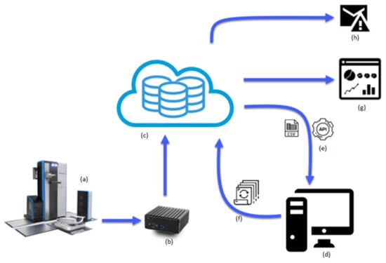
Figure 1.
Architecture diagram of the infrastructure implemented.
3. Methods
This section is divided in two parts. First, in Section 3.1 we describe the methodology used to segment the data as a previous step to apply more complicated models. Then, in Section 3.2, we explain the techniques applied to gain a better knowledge about machine data. The analysis is based on dividing machine programs into operations and studying the resultant time series. In recent years, time series techniques have begun to be used in the context of machine tools [16,17].
3.1. Data Segmentation
From the division of variables in Section 2.1 the value of the second group of variables should arise from a combination of the value of the first group variable and the state of the machine and its different components, that is, there must be some function f such that
It seems clear then that under a similar machine state, the same values of user-defined variables should lead to similar values of analog-input variables. In other words, under the same machine state, performing the same operation should lead the machine to behave in the same way. As a consequence, if similar operations lead to different behavior, it can be taken as a sign of a change in machine state, usually due to component and tool wear.
The machining process is defined by a CNC program written in the ISO-6983 programming language Heidenhain–Klartext [18,19]. The name of the program being run is stored in the variable Cnc_Program_Name_RT. A CNC program is a list of commands that are executed one line (also called blocks) at the time. The number of program line being executed at each moment is stored in the variable Cnc_Program_BlockNumber_RT.
The program execution is sequential unless any control command forces the execution to jump lines. Additionally, since these programs are executed under operator supervision, the machining process can occasionally be stopped, or some parts might be re-run. The evolution of the block number in time during the execution of different programs can be seen in Figure 2a.
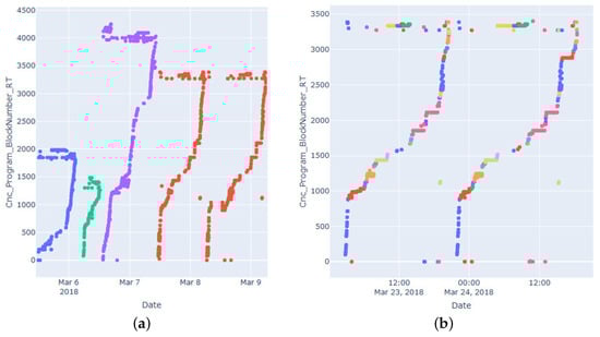
Figure 2.
(a) Evolution in time of Cnc_Program_BlockNumber_RT. (b) Segmentation of two executions of the same program by operation.
As can be seen, there are many sub-sequences that look to be monotonously increasing most of the time, while occasionally the numbers go back and forth, or some parts need to be re-run.
While it might seem a good idea to run comparisons of machine operations by block (that is, comparing executions of the same block of the same program), it is not practical since in many occasions the execution of a block is too short to be significant, sometimes being even too short to be captured by the sampling rate. That, combined with the high volatility of many analog-input variables, makes the block not a good base for comparison. As a solution we propose a new base for comparison in between block and program execution, called operation.
During the machining of large pieces that involve many different operations, it is required to change the tool attached to the spindle many times. These tools are identified by a code number, that is stored in the variable Cnc_Tool_Number_RT.
The machine is considered to be in production if the axes are moving or the spindle is spinning or the axes are moving, along with the program name being non-null and the block and tool number being neither null nor zero.
Then, an operation is defined as a sequence of time where
- the program name does not change,
- the tool number does not change, and
- the machine does not stay without production for more than 600 seconds.
Once divided the machine data in operation, an operation is determined by its program name, its tool number and the block numbers comprised along its duration. An operation is characterized as follows:
Two operations and are said to be operations of the same type if the three following conditions are fulfilled:
- (same program),
- (same tool), and
- (intersection of block extrema intervals).
This last condition needs to be met because, due to sampling rate and possible variations in program execution, the sequences of blocks are not likely to be exactly the same, and actually might have serious discrepancies while being the same operation. The fact that the block sequence is usually increasing and monotonous which is why the condition make sense the way it is posed.
In Figure 2b the way it is segmented can be seen. Each execution is segmented as sequences of blocks that are usually consecutive with the same tool. When we compare the segmentation between the two executions, similar sequences of blocks are executed with the same tool, so those sequences executed with the same tool are operations of the same type.
3.2. Overview of Techniques
This work focuses on studying the variable Spindle_Power_percent. This variable represents the percentage of electrical power that is using the Spindle with respect to its nominal power (in this particular case, 81 kW).
The electrical power used by a component it is usually a good indicator of its health, since under similar circumstances the consumption should be similar, and deviations from the norm might be an indicator of something going wrong (as for instance, a component engine failure or component wear).
After several executions of the same program have been performed and divided into operations, different executions of operations of the same time can be grouped and compared in order to establish which executions differ from the norm.
For that purpose, a distance matrix between different executions can be computed using the DTW algorithm, and then hierarchical clustering algorithms can be applied to that distance matrix. Then, clustering techniques are used on this distance matrix to establish whether an execution can be considered anomalous with respect to the others.
3.2.1. Dynamic Time Warping
DTW [20] is an algorithm used to measure the dissimilarity between two ordered sequences or time series that might vary in length and phase.
Having two ordered sequence (or time series) and , we define an alignment between U and V as a set of tuples with and that fulfills the following conditions:
- ,
- ,
- if , if and , then and
- if , if and , then .
Each possible alignment is a possible way of mapping two ordered sequences or time series in a scenario where differences in length or phase might make a direct matching point to point non appropriate. Depicting an alignment between two series as in Figure 3, the two last conditions imposes that any pair of segments should never cross.
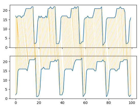
Figure 3.
Example of optimal alignment between two time series.
Then, if is the set of all the possible alignments between U and V, the DTW distance between U and V is
that is, the minimal sum of difference of elements in an alignment. In Figure 3 the optimal alignment between two time series is shown. Their DTW distance would be the sum of the difference in the absolute value of each pair of mapped points.
3.2.2. Hierarchical Clustering Techniques
Clustering techniques [21] are used to divide sets of elements into a subsets such that the elements in each subset are similar according to some criterion.
This work uses an agglomerative hierarchical clustering algorithm. It is an iterative algorithm that works as follows: Let us have a set S of elements to be divided into clusters. A family of subsets is a partition into clusters of S if they are mutually disjointed and their union is equal to S. A distance function
is defined for each pair of subsets of S. This function is called the linkage function of the algorithm. Then, the algorithm goes as follows:
- It starts from a partition of S where each element of S forms a single cluster.
- Each step it takes the two clusters for which D is minimized and combine them into a single cluster. If there is more than one possible choice, select randomly.
- Repeat until there is a single cluster that contains the whole set S.
Once this is done, S can be divided into k clusters by undoing the last steps of the algorithm. This is equivalent to just running the algorithm until the data has been grouped into k clusters but usually is necessary to run the algorithm to its end to see the bigger picture and decide how many natural clusters there are.
In a single-linkage clustering the linkage function is the following:
where d is some distance function for two elements of S (in this paper, d will be the DTW). That is, the single-linkage distance between two sets is the minimum distance between one element of one set and one element of the other.
A hierarchical clustering is usually represented visually through a dendogram, where it is easily seen which two clusters are joined together in each step, and what was the value of the linkage function at each union. The value of the linkage for each union is called the height of the dendogram. If S has N elements, denotes the height of the dendogram for each step of the algorithm, having a total of heights. This sequence is strictly non-decreasing.
Usually, when visually inspecting a dendogram, one can see many low heights and a few high heights. A rule of thumb in determining how many clusters there are is the number of high heights plus one. If there are no heights that are notably higher than most of them the data can be considered to form a unique cluster.
In Figure 4a is an example of clusterization with single-linkage, each color representing a cluster. In Figure 4b, we see the dendogram, where the black line represents the cut-off point.
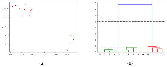
Figure 4.
(a) Example of clusterization by single linkage. (b) Dendogram and cut-off point.
3.3. Anomaly Detection
For each execution of a program, its operations are analyzed [22] by comparing them with the previous execution of that operation. An execution is anomalous with respect to the previous ones by using this criterion: Let be a sequence of time series belonging to different executions of operations of the same type, and let be the ordered set of heights of the dendogram resulting from applying the single-linkage clustering algorithm to these series. Then, is anomalous with respect to the previous one if the following two conditions apply:
- After dividing S in two clusters, is alone in one cluster and the rest are in the other.
- is anomalous with respect to . A good criteria is that is anomalous if where and are the mean value and standard deviation of . The scalar is chosen according to Chebyshev’s inequality, by which, if comes from the same distribution as the rest of ’s, its probability of being outside is smaller than 0.1.
Then is added to the set of previous series if it is not anomalous, using it as a frame of comparison for future executions.
4. Results
The methodology described above is applied to a machine in real production. It machines a total of two different types of pieces. Each of these utilize two programs, one per side. In this section we show two examples of the application of the previous methodology to these data. The Python code necessary to replicate these results, as well as the data are fully available at [23].
In Figure 5a, eight executions of a finishing operation are analyzed. The value of the spindle power along its executions is similar, and the algorithm does not detect it as an anomaly since the last (the pink one at the top) execution would not be the only element in its cluster. In Figure 6a, the evolution in time of the spindle power for each series is compared, where the red one is the last to take place.
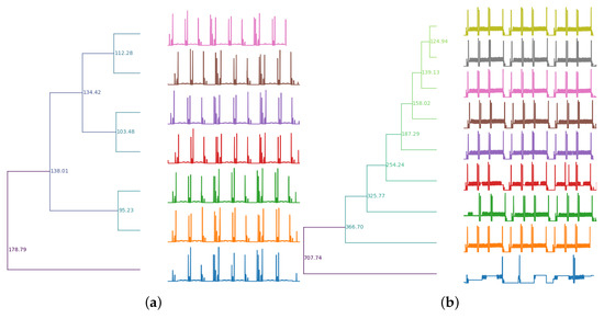
Figure 5.
(a) Example of analysis with no anomalous executions. (b) Example of analysis with one anomaly.
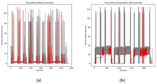
Figure 6.
(a) Spindle power during executions with no anomalies. (b) Spindle power for executions where one is anomalous.
On Figure 5b, eight executions of a sequence of drilling are analyzed. It can be seen as the last execution and is clearly anomalous with respect to the previous ones, as the pattern of spindle power is totally different. The algorithm detects the last execution as a clear anomaly, since the last execution (the blue one at the bottom) would be the only element in its cluster in a partition in two clusters of the sets, and its height is anomalous with respect to the previous ones, most likely due to a change of pattern. In Figure 6b, the evolution in time of the spindle power for each series is compared, where the red one is the last to take place and clearly anomalous. In this case a notification would have been issued.
5. Discussion
This work presents an innovative technique for early anomaly detection in the field of manufacturing. This novelty covers two fields: The algorithm for the segmentation of machine data into operations and the algorithm for anomaly detection itself.
Regarding the segmentation algorithm based on the collection of CNC information (program, line number, tool in use, and so on), this work has the advantage over previous works of data analysis in manufacturing as they usually depart from a conveniently segmented and labeled set of data (see, for instance [12]). In practice, it is unusual to depart from a duly labeled and segmented data set. This might happen for several reasons: lack of communication between data analyst and machine user, absence of necessary variables (for instance, a part counter), machining context where additional sub-segmenting is needed (a 10-second chain-production operation is not the same as a 3-min operation inside a 2-hour long process, where additional segmenting as it is done in this work is needed), etc. To the best of our knowledge, the problem of segmenting the data from the CNC has not yet been solved in the literature. We consider data segmentation very relevant as prior data preprocessing is a crucial, and often overlooked, aspect of data analytics.
Regarding the problem of anomaly detection for collections of time series, the problem has also been studied in the field of commercial software solutions [11] and academic research [12,13,14,15]. What these previous works have in common is their approach based on the extraction of features from the time series and performing data analysis on those features. For example, in [12] (and in the work upon which it is based, [13]) it is suggested to extract a set of very elaborated characteristics from each time series, reducing an object that could potentially have many dimensions to a collection of a few. Dimensions are reduced again via principal components analysis to avoid the curse of dimensionality. Additionally, density based algorithms for anomaly detection, such as DBSCAN [24], have been used to point out anomalous instances. The authors in [14] computed a selection of simpler features (absolute mean, kurtosis, and crest factor). From those statistics, a system of thresholds was established to determine anomalies. The researchers in [15] included in their analysis, features such as variance, crest factor, skewness, and wavelet energy. Using those previously mentioned features, the authors proposed a supervised problem where the data is analyzed towards the identification of a collection of known types of failures. As a main difference to those previous mentioned works, our technique is not based on feature extraction to compare series of data. We use instead, the whole time series. The main innovation of this paper with respect to the aforementioned previous ones is that, to the best of our knowledge, there is no similar approach in the literature in the field of manufacturing.
These previously published works have some advantage with respect to our approach: They are faster at computing (the DTW algorithm is with respect to the length of the time series, and our method is also with respect to the number of series) and they require less space to store the information about previous series (an array of statistics takes less space than the whole series). This advantage is becoming less meaningful in the context of Big Data since the ability to store and efficiently process large amounts of data makes our approach feasible. On top of that, manufacturers usually provide guidelines regarding hours of use for tools, so it is possible to determine after how many hours of use the machine data ceases to be comparable, allowing the possibility of "forgetting" time series that are too old.
On the other hand, the type of approach found in the literature has one big disadvantage with respect to the one proposed: By reducing each time series to a collection of statistics, many properties are lost. While the previously mentioned approaches are suitable for our purposes, and they do indeed do a good job by detecting the anomalies in our examples, it might happen that two time series are indeed very different but have very similar features. For example, let us have the collection of time series
and
where are independent random variables with distribution . That is, the seven first series are slightly perturbed sine signals, stretched to 1000 s, while the last one is a slightly perturbed, stretched cosine signal. In Figure 7a it can be seen how the cosine (in red) is clearly different to the sines (in red). However, in Figure 7b it is shown the result of selecting a set of key features [12] to this collection of series and then reducing the dimension by robust principal components analysis [25] and applying highest density region [26] as suggested by [13]. In this plot, the ten series that are more anomalous according to the application of the method are painted in red, and the cosine (painted in green) is not among them. On the other hand, in Figure 8 it can be seen that the result of applying the method proposed in this paper to the same collection of time series: The cosine stands out clearly as an anomaly.
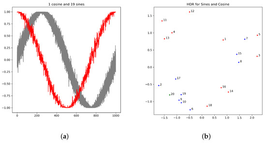
Figure 7.
(a) Representation of the one cosine (red) and nineteen sines (grey). (b) Application of [12] to these series.
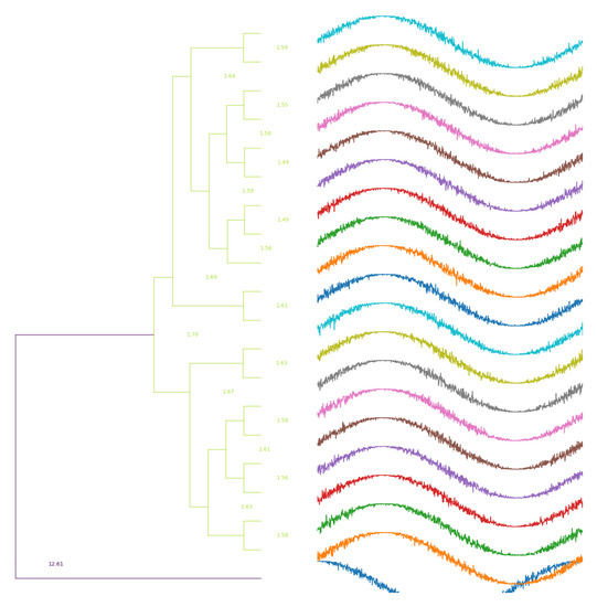
Figure 8.
Application of the method proposed in this work for one cosine and nineteen sines.
These two parts of the work combined have proven to be useful in production environments where machine failures and deviations in the production process are common, since the ability to detect these anomalies automatically allows taking action. In such problematic production environments, an algorithm like this may increase the production by handling unexpected situations more quickly.
It is relevant to remark on two possible limitations of this work:
- The first limitation of this methodology is the assumption that the machine user is going to always use the machine the same way. If the machine user follows best practices, changes in the CNC program should imply a new release and a new program name where the release number is indicated, however, this cannot always be assured. This situation could lead to misclassification of operations, and therefore to false negatives or false positives when detecting anomalous behaviors. As long as good practices are followed, this algorithm should be robust enough to be trusted.
- Another limitation of this work (and a path for possible future work) comes from the batch-like nature of the architecture. Data are downloaded and operations are segmented each number of minutes, and an operation is only analyzed (that is, compared with previous executions of the same operation) when it has finished. Due to this, if a very severe anomaly takes place, it might take some minutes until the system detects it. Regarding this limitation, when very severe anomalies happen there are usually other ways to be aware of them, including manual thresholds; the main target of this approach is to detect changes that might not be severe per se, but do imply a change in the way the machine is working, so the gap of a few minutes until it is detected does not make a large difference.
6. Conclusions and Future Work
The most relevant conclusions obtained from the work done and shown in this paper are:
- The developed methodology introduced in this paper takes industrial manufacturing a step further towards the Smart manufacturing and the Industry 4.0 paradigm.
- It allows machine operators to obtain a nearly real-time diagnosis of the production process.
- It permits a thorough scrutiny of so far unsupervised production parameters either pneumatic, hydraulic and/or electronic as far as production information can be analyzed and consolidated from an assortment of sensors.
- Rapid differentiation between anomalous and normal manufacturing processes is made possible via comparison between nearly real-time collected data and stored sequences from previous manufacturing cycles or theoretical ones developed by the hardware vendors.
- Manufacturing equipment can be preventively maintained as production anomalies are detected in advance.
- Collaborative manufacturing, one of the most important aims of Smart manufacturing and Industry 4.0, is put forward by the methodology summarized in this article.
Following the line of work on which the project is based, while seeing that the analysis of time series in industrial environments is beginning to be exploited, and seeing the capabilities it offers, the following tasks are proposed as future work:
- Apply the knowledge acquired during the pattern detection process, which allows the detection of other behaviors, anomalies or wear, in critical elements of the machine and therefore allows for the avoidance of unscheduled stops or long periods of inactivity of the machine.
- Improvement of the visualization is proposed, adapting more to the process focusing on the operator at the foot of the machine, allowing him to have a diagnosis at all times.
- Validate the model when there is no continuity in the processes, that is, when serial pieces are not made. By having more diverse information, there is not so much specific information about the process, which can be a great barrier to developing a reliable model.
- Use mixed models of deep learning and machine learning and combining them with DTW to improve the model, as well as different methodologies that can be adjusted to the problems that may appear.
- Using deep learning techniques to be able to implement a predictive model. Currently making a predictive model in real time is very complex due to the limitations offered by the numerical control. It must be taken into account that it is not the task of the CNC to have to perform such tasks.
- In order to improve the response time to anomalies, early classification techniques for time series [27] will be considered so that anomalous behavior can be detected before the operation has finished.
Author Contributions
Conceptualization: A.A. (Amaia Arregi) and J.E.; data curation: G.H.; formal analysis: J.E. and G.H.; investigation: G.H.; project administration: A.A. (Alfonso Antolínez), J.K.G.; software: G.H.; supervision: A.A. (Alfonso Antolínez), J.K.G.; validation: J.E.; visualization: J.E. and G.H.; writing—original draft preparation: J.E. and G.H.; writing—reviewing & editing: A.A. (Alfonso Antolínez), J.E. and G.H.
Funding
This research received no external funding.
Conflicts of Interest
The authors declare no conflict of interest.
Abbreviations
The following abbreviations are used in this manuscript:
| API | Application Programming Interface |
| CNC | Computer Numerical Control |
| DBSCAN | Density-Based Spatial Clustering of Applications with Noise |
| DTW | Dynamic Time Warp |
| IIoT | Industrial Internet of Things |
| IoT | Internet of Things |
| PLC | Programmable Logic Controller |
References
- Moldovan, L.; Gligor, A. Foreword Global trends in manufacturing technologies which create a path to tomorrow’s innovations. Procedia Manuf. 2018, 22, 1–3. [Google Scholar] [CrossRef]
- Directorate-General Internal Market, Industry, E.; SMEs. Digital Transformation Monitor Germany: Industrie 4.0; Technical Report; European Comission: Brussels, Belgium, 2017. [Google Scholar]
- Schleinkofer, U.; Klöpfer, K.; Schneider, M.; Bauernhansl, T. Cyber-physical Systems as Part of Frugal Manufacturing Systems. Procedia CIRP 2019, 81, 264–269. [Google Scholar] [CrossRef]
- Vaidya, S.; Ambad, P.; Bhosle, S. Industry 4.0—A Glimpse. Procedia Manuf. 2018, 20, 233–238. [Google Scholar] [CrossRef]
- Boyes, H.; Hallaq, B.; Cunningham, J.; Watson, T. The industrial internet of things (IIoT): An analysis framework. Comput. Ind. 2018, 101, 1–12. [Google Scholar] [CrossRef]
- Aberdeen Group; Cline, G. Towards Industry 4.0: An Overview of European Strategic Roadmaps; Technical Report; IBM: Aberdeen, UK, 2010. [Google Scholar]
- Santos, C.; Mehrsai, A.; Barros, A.; Araújo, M.; Ares, E. Towards Industry 4.0: An overview of European strategic roadmaps. Procedia Manuf. 2017, 13, 972–979. [Google Scholar] [CrossRef]
- Gerrikagoitia, J.; Unamuno, G.; Urkia, E.; Serna, A. Digital Manufacturing Platforms in the Industry 4.0 from Private and Public Perspectives. Appl. Sci. 2019, 9, 2934. [Google Scholar] [CrossRef]
- Dalenogare, L.S.; Benitez, G.B.; Ayala, N.F.; Frank, A.G. The expected contribution of Industry 4.0 technologies for industrial performance. Int. J. Prod. Econ. 2018, 204, 383–394. [Google Scholar] [CrossRef]
- Lee, J.; Kao, H.A.; Yang, S. Service Innovation and Smart Analytics for Industry 4.0 and Big Data Environment. Procedia CIRP 2014, 16, 3–8. [Google Scholar] [CrossRef]
- Detecting CNC Anomalies with Unsupervised Learning (Part 1). Available online: https://medium.com/machinemetrics-techblog/using-pca-and-clustering-to-detect-machine-anomalies-part-1-ba89f6a6a8cd (accessed on 6 November 2019).
- Zhang, L.; Elghazoly, S.; Tweedie, B. Introducing AnomDB: An Unsupervised Anomaly Detection Method for CNC Machine Control Data. Proc. Annu. Conf. PHM Soc. 2019, 11. [Google Scholar] [CrossRef]
- Hyndman, R.J.; Wang, E.; Laptev, N. Large-Scale Unusual Time Series Detection. In Proceedings of the 2015 IEEE International Conference on Data Mining Workshop (ICDMW), Atlantic City, NJ, USA, 14–17 November 2015; pp. 1616–1619. [Google Scholar] [CrossRef]
- Liang, Y.; Wang, S.; Li, W.; Lu, X. Data-Driven Anomaly Diagnosis for Machining Processes. Engineering 2019, 5, 646–652. [Google Scholar] [CrossRef]
- DEmilia, G.; Gaspari, A.; Hohwieler, E.; Laghmouchi, A.; Uhlmann, E. Improvement of Defect Detectability in Machine Tools Using Sensor-based Condition Monitoring Applications. Procedia CIRP 2018, 67, 325–331. [Google Scholar] [CrossRef]
- Żabiński, T.; Mączka, T.; Kluska, J.; Madera, M.; Sep, J. Condition monitoring in Industry 4.0 production systems—The idea of computational intelligence methods application. Procedia CIRP 2019, 79, 63–67. [Google Scholar] [CrossRef]
- Yin, S.; Ding, S.X.; Xie, X.; Luo, H. A Review on Basic Data-Driven Approaches for Industrial Process Monitoring. IEEE Trans. Ind. Electron. 2014, 61, 6418–6428. [Google Scholar] [CrossRef]
- Klartext Portal. Available online: https://www.klartext-portal.com (accessed on 23 October 2019).
- ISO 6983-1:2009. Available online: https://www.iso.org/standard/34608.html (accessed on 23 October 2019).
- Jeong, Y.S.; Jeong, M.K.; Omitaomu, O.A. Weighted dynamic time warping for time series classification. Pattern Recogn. 2011, 44, 2231–2240. [Google Scholar] [CrossRef]
- Maimon, O.; Rokach, L. Data Mining and Knowledge Discovery Handbook, 2nd ed.; Springer: New York, NY, USA, 2010. [Google Scholar]
- Lin, J.; Williamson, S.; Borne, K.; DeBarr, D. Pattern Recognition in Time Series. Adv. Mach. Learn. Data Min. Astron. 2012, 1, 617–645. [Google Scholar] [CrossRef]
- Git Repository for This Work. Available online: https://gitlab.danobatgroup.com/gherranz/pattern-recognition (accessed on 29 November 2019).
- Ester, M.; Kriegel, H.P.; Sander, J.; Xu, X. A Density-based Algorithm for Discovering Clusters a Density-based Algorithm for Discovering Clusters in Large Spatial Databases with Noise. In Proceedings of the Second International Conference on Knowledge Discovery and Data Mining; AAAI Press: Palo Alto, CA, USA, 1996; pp. 226–231. [Google Scholar]
- Candès, E.J.; Li, X.; Ma, Y.; Wright, J. Robust Principal Component Analysis? J. ACM 2011, 58, 11:1–11:37. [Google Scholar] [CrossRef]
- Hyndman, R.J. Computing and Graphing Highest Density Regions. Am. Stat. 1996, 50, 120–126. [Google Scholar] [CrossRef]
- Mori, U.; Mendiburu, A.; Miranda, I.; Lozano, J. Early classification of time series using multi-objective optimization techniques. Inf. Sci. 2019, 492, 204–218. [Google Scholar] [CrossRef]
© 2019 by the authors. Licensee MDPI, Basel, Switzerland. This article is an open access article distributed under the terms and conditions of the Creative Commons Attribution (CC BY) license (http://creativecommons.org/licenses/by/4.0/).