Figure 1.
Key elements considered for the benchmarking design approach, adapted from [
27].
Figure 1.
Key elements considered for the benchmarking design approach, adapted from [
27].
Figure 2.
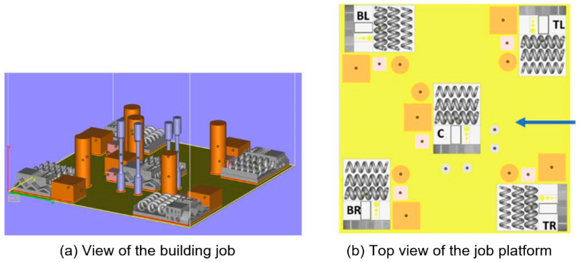
View of one complete platform of benchmarking building job. (
a) View of the full building job; (
b) Top view of the building platform [
27].
Figure 2.
View of one complete platform of benchmarking building job. (
a) View of the full building job; (
b) Top view of the building platform [
27].
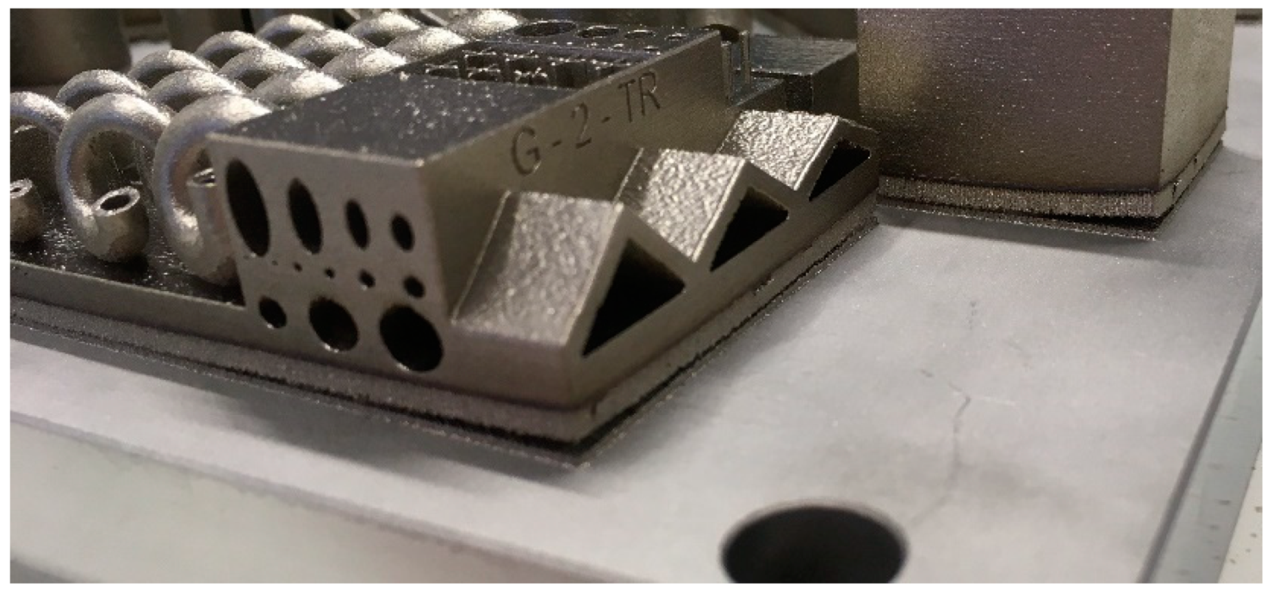
Figure 3.
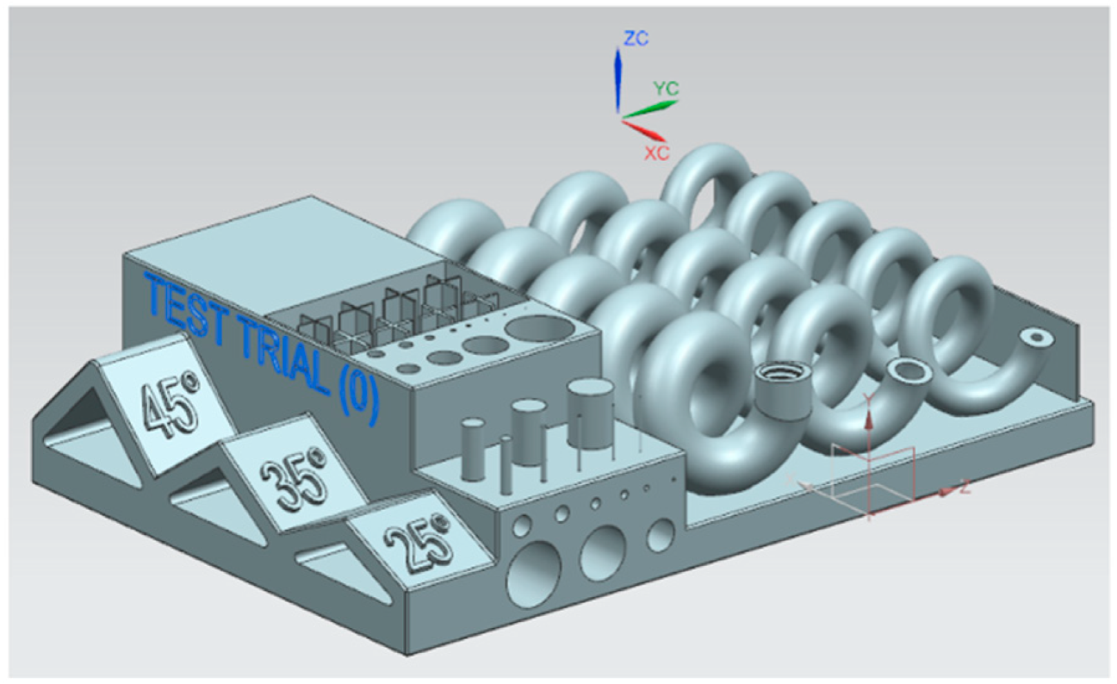
Artifact with spiral on benchmarking [
27].
Figure 3.
Artifact with spiral on benchmarking [
27].
Figure 4.
Surface roughness measurements of samples with spiral and big parallelepiped. (left) position on the sample with spirals where the roughness in X and Y directions was measured, (right) position on the parallelepiped where the roughness in Z and T directions was measured.
Figure 4.
Surface roughness measurements of samples with spiral and big parallelepiped. (left) position on the sample with spirals where the roughness in X and Y directions was measured, (right) position on the parallelepiped where the roughness in Z and T directions was measured.
Figure 5.
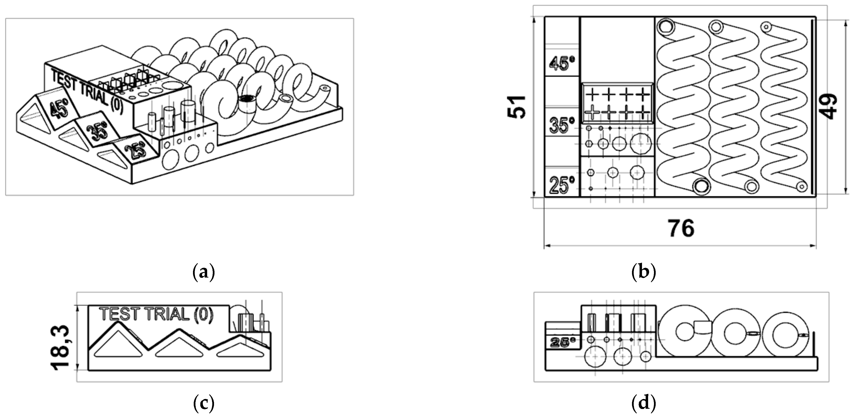
Nominal CAD drawings with reference dimensions. (a) isometric view, (b) top view, (c) left side view, (d) front view.
Figure 5.
Nominal CAD drawings with reference dimensions. (a) isometric view, (b) top view, (c) left side view, (d) front view.
Figure 6.
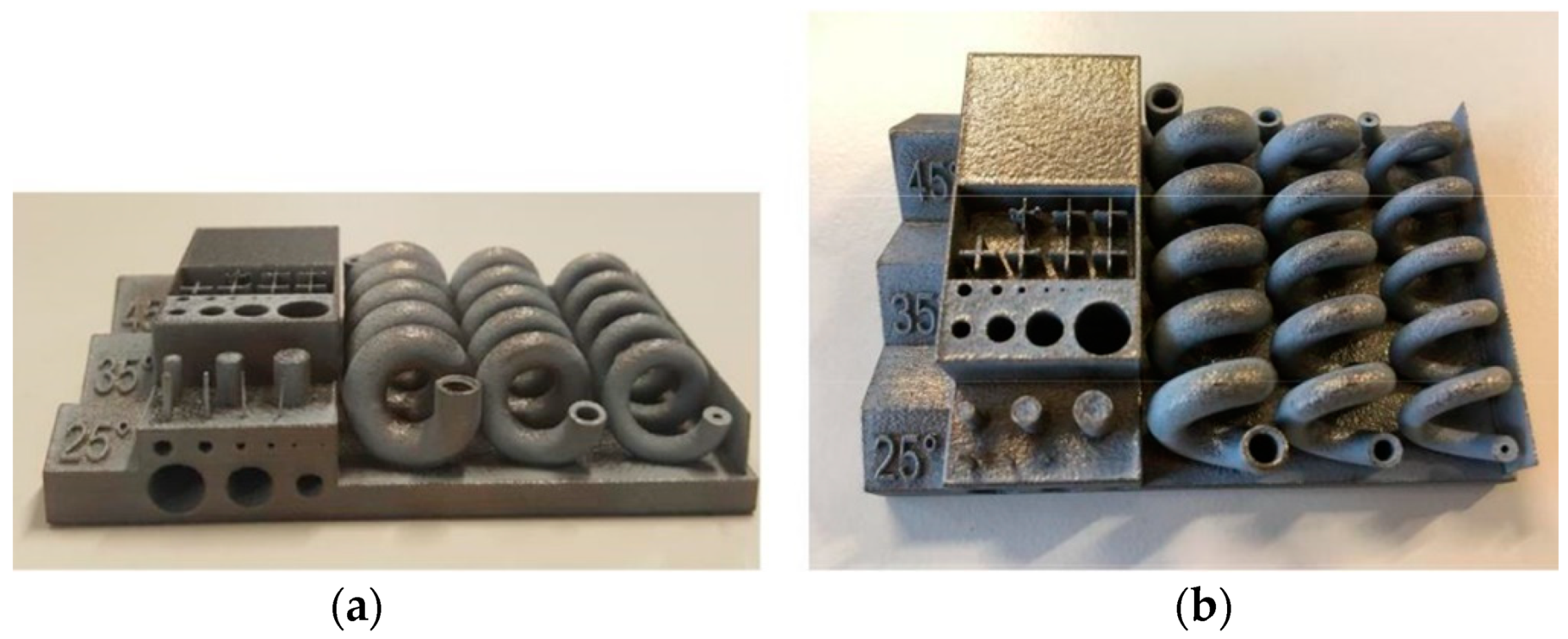
Views of samples received from company B. (a) front view, (b) top view.
Figure 6.
Views of samples received from company B. (a) front view, (b) top view.
Figure 7.
Views of samples received from company H. (a) front view, (b) top view.
Figure 7.
Views of samples received from company H. (a) front view, (b) top view.
Figure 8.
Delamination visible on the sample from company G.
Figure 8.
Delamination visible on the sample from company G.
Figure 9.
3D scanner alignment used for the evaluation of the results: view of alignment on spirals (left), and on the top (right).
Figure 9.
3D scanner alignment used for the evaluation of the results: view of alignment on spirals (left), and on the top (right).
Figure 10.
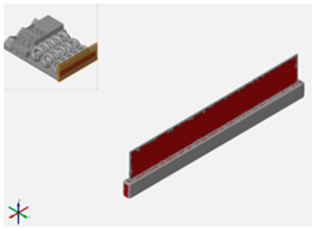
View of alignment on the thin wall.
Figure 10.
View of alignment on the thin wall.
Figure 11.
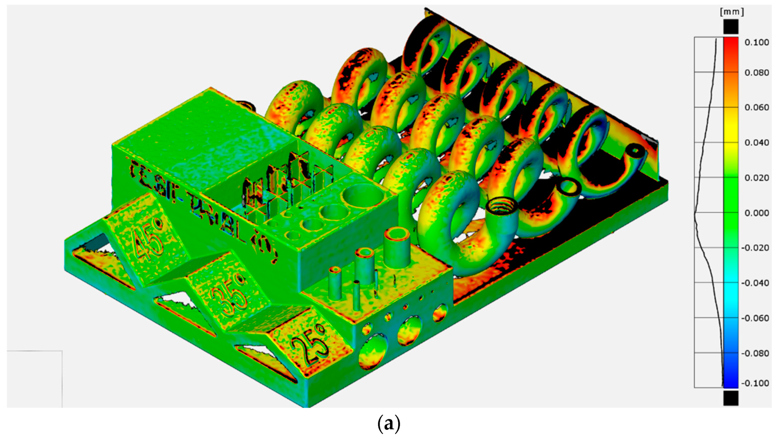
Color plot of the central spiral sample, first job from company H.
Figure 11.
Color plot of the central spiral sample, first job from company H.
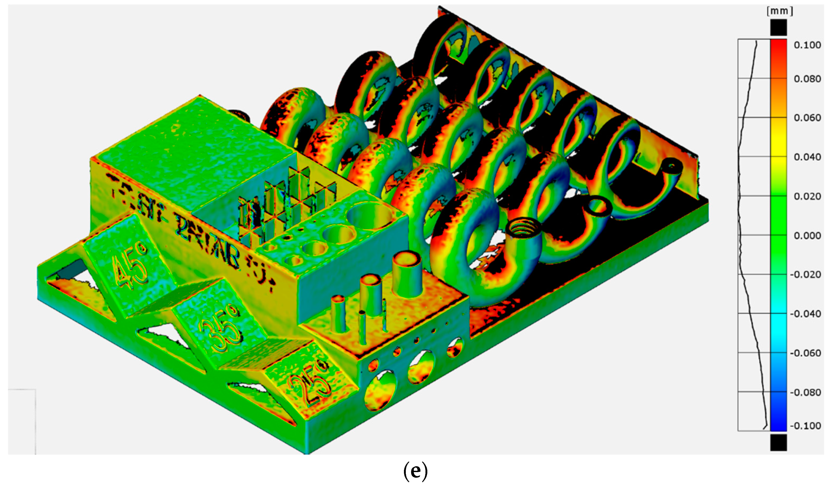
Figure 12.
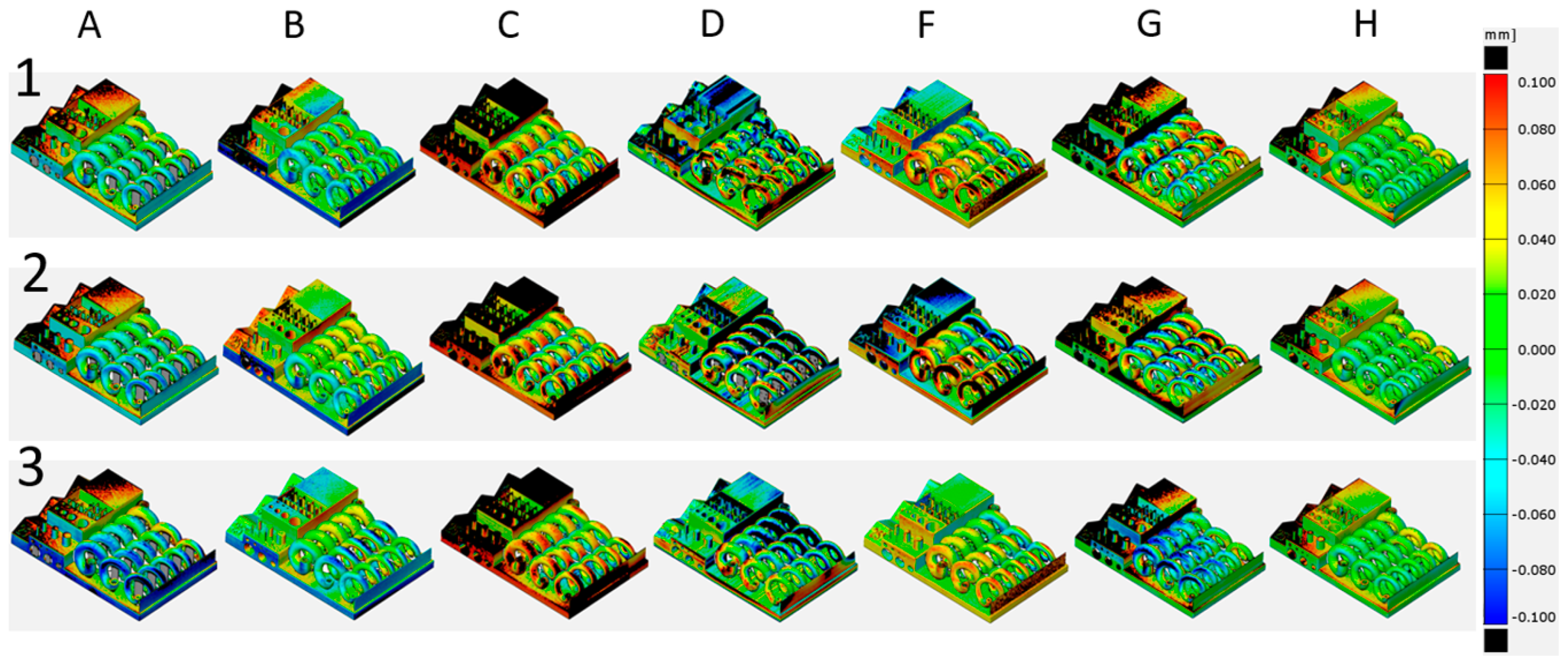
Comparison of color plots from the central sample of each benchmarking job. Job number is on the left (1, 2 and 3); letter on top represents participant (A, B, C, D, F, G and H); color scale is on the right.
Figure 12.
Comparison of color plots from the central sample of each benchmarking job. Job number is on the left (1, 2 and 3); letter on top represents participant (A, B, C, D, F, G and H); color scale is on the right.
Figure 13.
Color plot of the entire first job from G, 3D scanner top alignment. (a) BL, (b) BR, (c) C, (d) TL, (e) TR.
Figure 13.
Color plot of the entire first job from G, 3D scanner top alignment. (a) BL, (b) BR, (c) C, (d) TL, (e) TR.
Figure 14.
Color plot from the entire second job from company H; 3D scanner top alignment. (a) BL, (b) BR, (c) C, (d) TL, (e) TR.
Figure 14.
Color plot from the entire second job from company H; 3D scanner top alignment. (a) BL, (b) BR, (c) C, (d) TL, (e) TR.
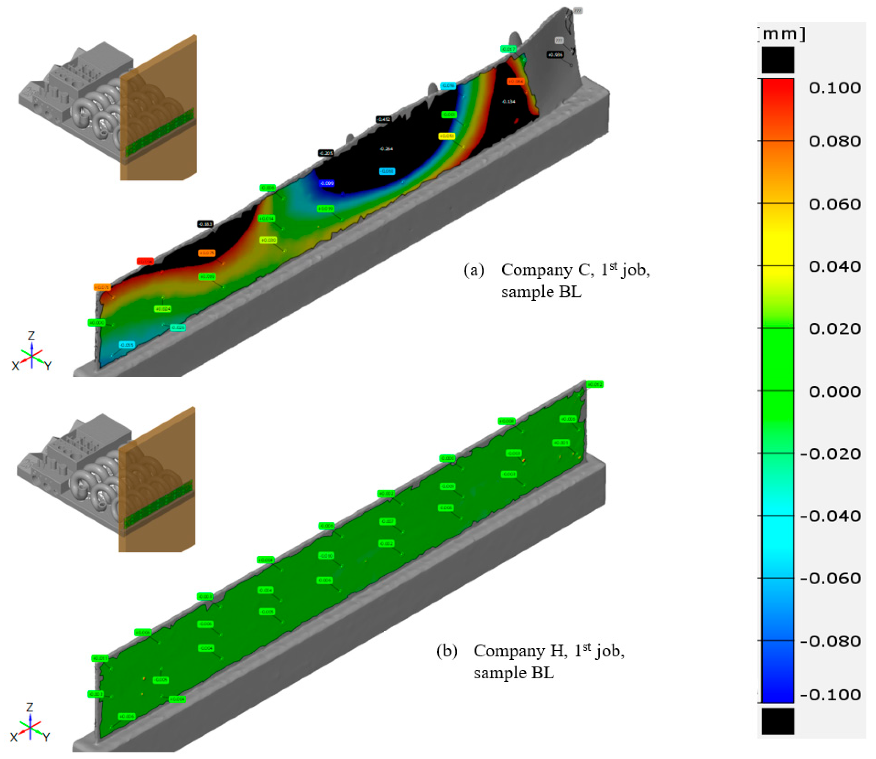
Figure 15.
Comparison of the thin wall color plots from companies C and H. (a) sample BL from company C, 1st job, (b) sample BL from company H, 1st job.
Figure 15.
Comparison of the thin wall color plots from companies C and H. (a) sample BL from company C, 1st job, (b) sample BL from company H, 1st job.
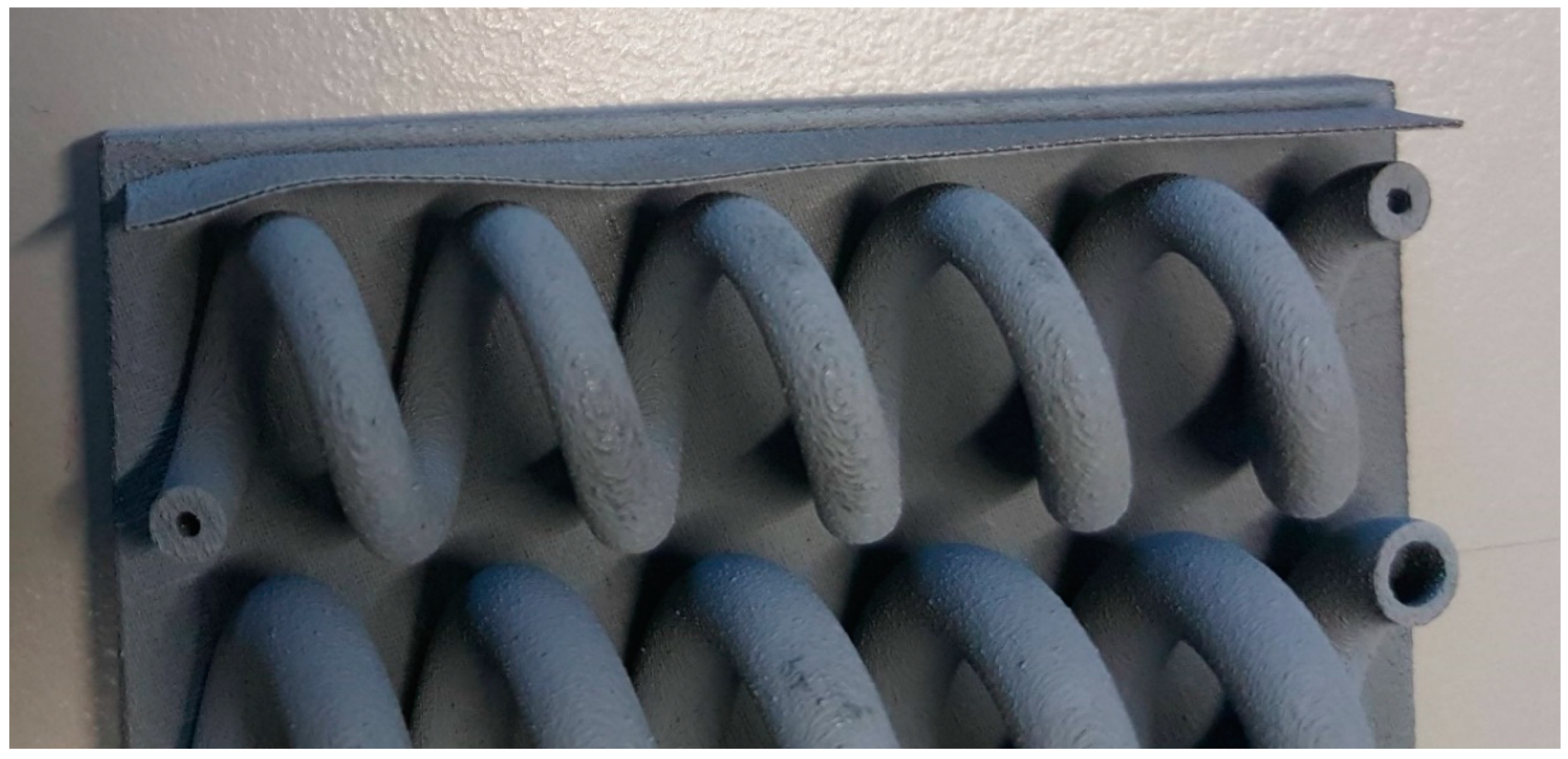
Figure 16.
Picture of the real sample from company C, first job, BL.
Figure 16.
Picture of the real sample from company C, first job, BL.
Figure 17.
Optical microscope analysis of 2 mm pins from selected participants.
Figure 17.
Optical microscope analysis of 2 mm pins from selected participants.
Figure 18.
Deviation graph of the pin diameters compared to nominal CAD dimension produced with GOM Inspect for each pin from each company (in the graph, company F is referred to as company I).
Figure 18.
Deviation graph of the pin diameters compared to nominal CAD dimension produced with GOM Inspect for each pin from each company (in the graph, company F is referred to as company I).
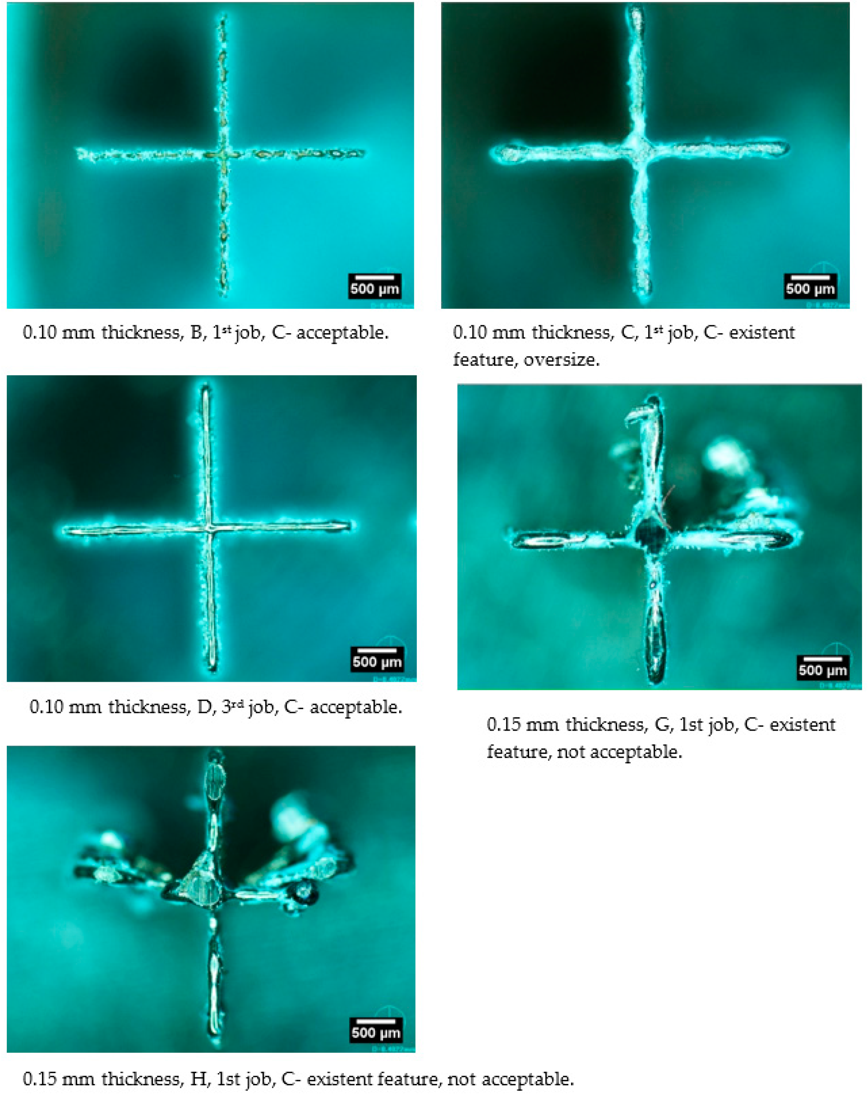
Figure 19.
Optical microscope analysis of 0.10 mm and 0.15 mm thick crosses from selected participants. Each picture presents a short description below.
Figure 19.
Optical microscope analysis of 0.10 mm and 0.15 mm thick crosses from selected participants. Each picture presents a short description below.
Figure 20.
Deviation graph of the cross wall thickness compared to the nominal CAD dimension produced with GOM Inspect for each cross from each company (in the graph, company F is referred to as company I).
Figure 20.
Deviation graph of the cross wall thickness compared to the nominal CAD dimension produced with GOM Inspect for each cross from each company (in the graph, company F is referred to as company I).
Figure 21.
Deviation graph of the hole diameters compared to nominal CAD dimensions produced with GOM Inspect for each hole from each company (in the graph, company F is referred to as company I).
Figure 21.
Deviation graph of the hole diameters compared to nominal CAD dimensions produced with GOM Inspect for each hole from each company (in the graph, company F is referred to as company I).
Figure 22.
Optical microscope pictures of selected holes: diameter of 1.5 mm and 1.2 mm, F, first job, central sample (left); diameter of 1.5 mm and 1.2 mm, H, first job, central sample (right).
Figure 22.
Optical microscope pictures of selected holes: diameter of 1.5 mm and 1.2 mm, F, first job, central sample (left); diameter of 1.5 mm and 1.2 mm, H, first job, central sample (right).
Figure 23.
Deviation graph of pyramid inclination measurements compared to the nominal CAD dimensions produced with GOM Inspect for each pyramid from each company (in the graph, company F is referred as company I).
Figure 23.
Deviation graph of pyramid inclination measurements compared to the nominal CAD dimensions produced with GOM Inspect for each pyramid from each company (in the graph, company F is referred as company I).
Figure 24.
Observed defects on the spiral samples: pyramids from company D, first job, C sample (left); recoater issue from company D, first job, T sample (right).
Figure 24.
Observed defects on the spiral samples: pyramids from company D, first job, C sample (left); recoater issue from company D, first job, T sample (right).
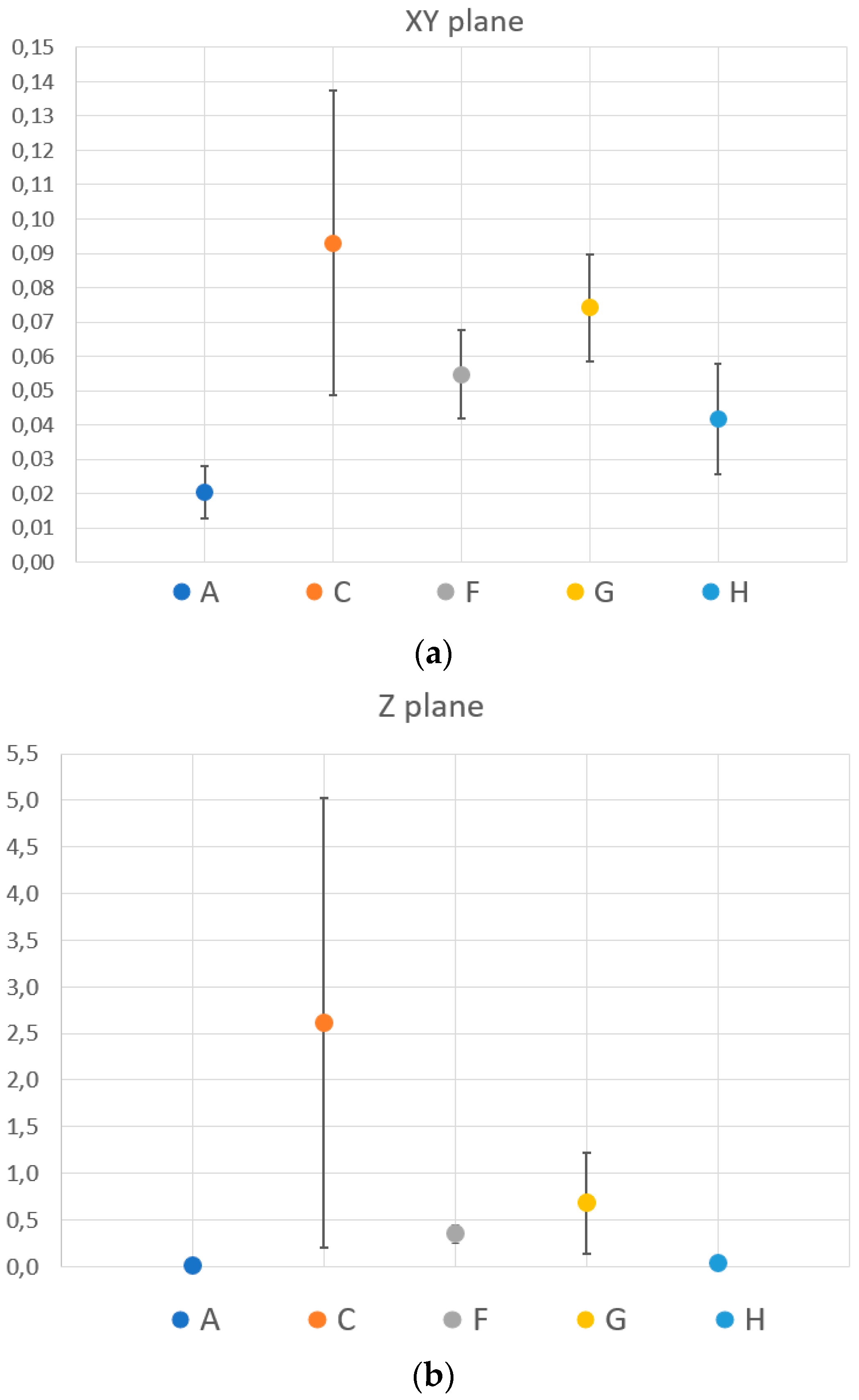
Figure 25.
Ra (μm) represents the comparison for each direction across players. Roughness on the (a) X, (b) Y, (c) Z, (d) T directions.
Figure 25.
Ra (μm) represents the comparison for each direction across players. Roughness on the (a) X, (b) Y, (c) Z, (d) T directions.
Figure 26.
Percentage of residual defects on the polished surfaces of the (a) XY, (b) XZ surfaces.
Figure 26.
Percentage of residual defects on the polished surfaces of the (a) XY, (b) XZ surfaces.
Figure 27.
Residual defect, company C: XY face (left), XZ face (right).
Figure 27.
Residual defect, company C: XY face (left), XZ face (right).
Figure 28.
Rockwell hardness C (HRC) values across the selected companies: XY face (left); XZ face (right).
Figure 28.
Rockwell hardness C (HRC) values across the selected companies: XY face (left); XZ face (right).
Figure 29.
Tall parts produced by selected companies: company A (left), company G (right).
Figure 29.
Tall parts produced by selected companies: company A (left), company G (right).
Table 1.
Examples of benchmarking of additive manufacturing (AM) technologies. For the AM technologies: SLA, stereolithography; SLS, selective laser sintering; LOM, laminated object manufacturing; FDM, fused deposition modeling.
Table 1.
Examples of benchmarking of additive manufacturing (AM) technologies. For the AM technologies: SLA, stereolithography; SLS, selective laser sintering; LOM, laminated object manufacturing; FDM, fused deposition modeling.
| Ref. | Year | AM Tech | Materials | Comments |
|---|
| [16] | 2004 | SLA, SLS, LOM, FDM | Different plastics | Comparative evaluation of AM processes, incorporating features from different benchmarking (dimensions: 170 × 170 × 20 mm). |
| [17] | 2005 | SLS, LPBF | Different metal alloys | Thin plate with multiple features (dimensions: 50 × 50 × 9 mm). |
| [18] | 2006 | SLS | Steel-based alloys | Design derived from a real component: half die of a glass bottle (dimensions: 200 × 100 × 40 mm). |
| [19] | 2006 | BJ | Different plastics | Development of a methodology to classify the accuracy of printed parts. |
| [20] | 2007 | LPBF | TiAl6V4 and Co–Cr–Mo | Investigation of medical parts production. |
| [21] | 2010 | SLS | Bronze-based metal | Same features repeated in different orientations in different positions (dimensions of small features: 20 × 20 × 20 mm). |
| [22] | 2010 | BJ | Mixture of polymers | Systematic investigation of the influence of 4 process parameters on the quality and accuracy of green parts. |
| [23] | 2011 | FDM | ABS | Quantitative evaluation of open-source 3D printer. |
| [24] | 2011 | MJ, SLA, SLS, FDM | Different plastics | Simple and quick method to compare speed and accuracy of AM technologies. |
| [25] | 2012 | SLS | Nylon | Focus on accuracy and repeatability (dimensions: 270 × 50 mm). |
| [14] | 2014 | Several AM techs | Several materials | Moylan et al.’s standardization proposal (dimensions: 100 × 100 × 10 mm). |
| [26] | 2015 | SLS, SLA, MJ | Different plastics | Definition of a DoE to optimize the manufacturing of a mass-production consumer device geometry. |
Table 2.
Investigation criteria of benchmarking.
Table 2.
Investigation criteria of benchmarking.
| General Aspect | Specification | Comments |
|---|
| Accuracy | Dimension of feature | Various features visible in Figure 3, with minimum dimensions that go beyond the currently known machine’s limitation (see Table 3). |
| Surface roughness | Important factor considering industrial production and current need for post-processing parts to achieve specified roughness. |
| Repeatability | Same job, different positions | Evaluated by repeating production of the same part in 4 corners of the machine’s building volume and centre of the building platform; extremely important considering industrial need for a robust and reliable process. |
| Different jobs | Same as above; each job repeated 3 times. |
| Complex feature | Spiral shape: mold’s cooling channel | Overview of machine capabilities in handling complex features that can be related to real applications such as conformal cooling channels in molds. |
| Homogeneity | Residual defects | Indicator of process quality. |
| Density |
| Residual stress | Part distortions | Related to robustness of the process and final quality of the product in terms of how close they are to the nominal design. |
| Mechanical properties | Rockwell hardness C | General indicator of quality of the material. |
| Built speed | | To compare the speed of various machines. |
| Tall parts production | Tall samples | Understanding of machine capabilities in building relatively tall parts. |
Table 3.
Minimum dimension of features presented in benchmarking artifact.
Table 3.
Minimum dimension of features presented in benchmarking artifact.
| Feature | Minimum Dimension | Min Dimension in Artifact |
|---|
| Wall thickness | 0.15 mm | 0.10 mm |
| Overhang structure | 45° | 25° |
| Circular holes (diameter) | 0.50 mm | 0.20 mm |
| Circular pins (diameter) | 0.50 mm | 0.10 mm |
Table 4.
Chemical composition of maraging steel (st-%) [
31].
Table 4.
Chemical composition of maraging steel (st-%) [
31].
| Fe | Ni | Co | Mo | Ti | Al | Cr, Cu | C | Mn, Si | P, S |
|---|
| Bal | 17–19% | 8.5–9.5% | 4.5–5.2% | 0.6–0.8% | 0.05–0.15% | Each ≤0.5% | ≤0.03% | Each ≤0.1% | Each ≤0.01% |
Table 5.
Surface roughness measurement specifications.
Table 5.
Surface roughness measurement specifications.
| Ra Range | 2–10 μm |
|---|
| Evaluation length | 12.5 mm |
| Sample length | 2.5 mm |
| λc | 2.5 mm |
| λf | 0.08 mm |
| Number of cut-offs | 5 |
| Surface | Aperiodic |
| Filter | Gaussian |
Table 6.
Machines evaluated in this benchmarking. Machine H is the only one whose information will be shared: Yb fiber laser, max power 200 W, building platform 250 × 250 mm, nitrogen atmosphere, hard ceramic recoater.
Table 6.
Machines evaluated in this benchmarking. Machine H is the only one whose information will be shared: Yb fiber laser, max power 200 W, building platform 250 × 250 mm, nitrogen atmosphere, hard ceramic recoater.
| Company | Type of Company | No. Lasers Used | Cutting Technology | Layer Thickness [μm] |
|---|
| A | Machine manufacturer | 1 | Wire EDM | 40 |
| B | Machine manufacturer | 1 | Wire EDM | 30 |
| C | Machine manufacturer | 2 | 2 jobs: wire EDM 1 job: band saw | 30 |
| D | Machine manufacturer | 1 | Wire EDM | 40 |
| E | End user (machine owner) | 2 | – | 40 |
| F | Machine manufacturer | 4 | Wire EDM | 40 |
| G | End user (machine owner) | 1 | Band saw | 40 |
| H | End user (machine owner) | 1 | Band saw | 40 |
Table 7.
Pin construction summary for each company. ✓ acceptable; ≈ uncertain; ✗ not built.
Table 7.
Pin construction summary for each company. ✓ acceptable; ≈ uncertain; ✗ not built.
| Supplier | Pin | 1 | 2 | 3 | 4 | 5 | 6 | 7 | 8 |
|---|
| A | TL | ✗✗✗ | ✗✗✗ | ✗✓✓ | ✗✗≈ | ✓✓✓ | ✓✓✓ | ✓✓✓ | ✓✓✓ |
| TR | ✗✗✗ | ✗✗✗ | ✗✓✗ | ✗✗≈ | ✓✓✓ | ✓✓✓ | ✓✓✓ | ✓✓✓ |
| C | ✗✗✗ | ✗≈✗ | ✓✓✓ | ✗≈✗ | ✓✓✓ | ✓✓✓ | ✓✓✓ | ✓✓✓ |
| BL | ✗✗✗ | ✗✗✗ | ✗✓≈ | ✗≈≈ | ✓✓✓ | ✓✓✓ | ✓✓✓ | ✓✓✓ |
| BR | ✗✗✗ | ✗✗✗ | ✓✗✓ | ✗✗✗ | ✓✓✓ | ✓✓✓ | ✓✓✓ | ✓✓✓ |
| B | TL | ✗≈✗ | ≈✗✗ | ✓✓✓ | ✓✓✓ | ✓✓✓ | ✓✓✓ | ✓✓✓ | ✓✓✓ |
| TR | ✗✗≈ | ≈≈≈ | ✓✓✓ | ✓✓✓ | ✓✓✓ | ✓✓✓ | ✓✓✓ | ✓✓✓ |
| C | ✗✗≈ | ≈≈≈ | ✓✓✓ | ✓✓✓ | ✓✓✓ | ✓✓✓ | ✓✓✓ | ✓✓✓ |
| BL | ✗≈✗ | ≈≈✗ | ✓✓✓ | ✓✓✓ | ✓✓✓ | ✓✓✓ | ✓✓✓ | ✓✓✓ |
| BR | ✗≈≈ | ≈≈≈ | ✓✓✓ | ✓✓✓ | ✓✓✓ | ✓✓✓ | ✓✓✓ | ✓✓✓ |
| C | TL | ≈≈≈ | ≈≈≈ | ✓✓✓ | ✓✓✓ | ✓✓✓ | ✓✓✓ | ✓✓✓ | ✓✓✓ |
| TR | ≈≈≈ | ≈≈≈ | ✓✓✓ | ✓✓✓ | ✓✓✓ | ✓✓✓ | ✓✓✓ | ✓✓✓ |
| C | ≈≈≈ | ≈≈≈ | ✓✓✓ | ✓✓✓ | ✓✓✓ | ✓✓✓ | ✓✓✓ | ✓✓✓ |
| BL | ≈≈≈ | ≈≈≈ | ✓✓✓ | ✓✓✓ | ✓✓✓ | ✓✓✓ | ✓✓✓ | ✓✓✓ |
| BR | ≈≈≈ | ≈≈≈ | ✓✓✓ | ✓✓✓ | ✓✓✓ | ✓✓✓ | ✓✓✓ | ✓✓✓ |
| D | R | ✗✗✗ | ≈✗✗ | ✓✓✓ | ✓✓✓ | ✓✓✓ | ✓✓✓ | ✓✓✓ | ✓✓✓ |
| T | ✗✗✗ | ✗≈✗ | ✓✓✓ | ✓✓✓ | ✓✓✓ | ✓✓✓ | ✓✓✓ | ✓✓✓ |
| C | ✗✗✗ | ✗✗✗ | ✓✓✗ | ✓✓✓ | ✓✓✓ | ✓✓✓ | ✓✓✓ | ✓✓✓ |
| L | ✗✗✗ | ✗✗≈ | ✓✓✓ | ✓✓✓ | ✓✓✓ | ✓✓✓ | ✓✓✓ | ✓✓✓ |
| B | ✗✗✗ | ✗✗✗ | ✓✓✗ | ✓✓✓ | ✓✓✓ | ✓✓✓ | ✓✓✓ | ✓✓✓ |
| F | TL | ✗✗✗ | ✗✗✗ | ✗✗✗ | ✓✓✓ | ✓✓✓ | ✓✓✓ | ✓✓✓ | ✓✓✓ |
| TR | ✗✗✗ | ✗✗✗ | ✓✗✓ | ✓✓✓ | ✓✓✓ | ✓✓✓ | ✓✓✓ | ✓✓✓ |
| C | ✗✗✗ | ✗✗✗ | ✓≈✗ | ✓✓✓ | ✓✓✓ | ✓✓✓ | ✓✓✓ | ✓✓✓ |
| BL | ✗✗✗ | ✗✗✗ | ✗✗✗ | ✓✓✓ | ✓✓✓ | ✓✓✓ | ✓✓✓ | ✓✓✓ |
| BR | ✗✗✗ | ✗✗✗ | ✓✓✓ | ✓✓✓ | ✓✓✓ | ✓✓✓ | ✓✓✓ | ✓✓✓ |
| G | TL | ✗✗✗ | ✗≈✗ | ✓✓✓ | ✓✓✓ | ✓✓✓ | ✓✓✓ | ✓✓✓ | ✓✓✓ |
| TR | ✗✗✗ | ✗✗✗ | ✓✓✓ | ✓✓✓ | ✓✓✓ | ✓✓✓ | ✓✓✓ | ✓✓✓ |
| C | ✗✗✗ | ✗✗✗ | ✓✓✓ | ✓✓✓ | ✓✓✓ | ✓✓✓ | ✓✓✓ | ✓✓✓ |
| BL | ✗✗✗ | ✗✗✗ | ✓✓✓ | ✓✓✓ | ✓✓✓ | ✓✓✓ | ✓✓✓ | ✓✓✓ |
| BR | ✗✗✗ | ✗≈≈ | ✓✓✓ | ✓✓✓ | ✓✓✓ | ✓✓✓ | ✓✓✓ | ✓✓✓ |
| H | TL | ✗✗✗ | ✗✗≈ | ✓✓✓ | ✓✓✓ | ✓✓✓ | ✓✓✓ | ✓✓✓ | ✓✓✓ |
| TR | ✗✗✗ | ≈≈✗ | ✓✗✓ | ✓✓✓ | ✓✓✓ | ✓✓✓ | ✓✓✓ | ✓✓✓ |
| C | ✗✗✗ | ✗✗✗ | ✓✓✓ | ✓✓✓ | ✓✓✓ | ✓✓✓ | ✓✓✓ | ✓✓✓ |
| BL | ✗✗✗ | ≈≈≈ | ✗✗✓ | ✓✓≈ | ✓✓✓ | ✓✓✓ | ✓✓✓ | ✓✓✓ |
| BR | ✗✗✗ | ✗≈✗ | ✓✓✗ | ✓✓✓ | ✓✓✓ | ✓✓✓ | ✓✓✓ | ✓✓✓ |
Table 8.
Cross construction summary for each company. ✓ acceptable; ≈ existing feature, oversize; ✓ existing feature, not acceptable; ✗ not built.
Table 8.
Cross construction summary for each company. ✓ acceptable; ≈ existing feature, oversize; ✓ existing feature, not acceptable; ✗ not built.
| Supplier | Cross | 1 | 2 | 3 | 4 | 5 | 6 | 7 | 8 |
|---|
| A | TL | ✗✗✗ | ✗✗✗ | ✓✓✓ | ✓✓✓ | ✓✓✓ | ✓✓✓ | ✓✓✓ | ✓✓✓ |
| TR | ✗✗✗ | ✗✗✗ | ✓✓✓ | ✓✓✓ | ✓✓✓ | ✓✓✓ | ✓✓✓ | ✓✓✓ |
| C | ✗✗✗ | ✗✗✗ | ✓✓✓ | ✓✓✓ | ✓✓✓ | ✓✓✓ | ✓✓✓ | ✓✓✓ |
| BL | ✗✗✗ | ✗✗✗ | ✓✓✓ | ✓✓✓ | ✓✓✓ | ✓✓✓ | ✓✓✓ | ✓✓✓ |
| BR | ✗✗✗ | ✗✗✗ | ✓✓✓ | ✓✓✓ | ✓✓✓ | ✓✓✓ | ✓✓✓ | ✓✓✓ |
| B | TL | ✓✓✓ | ✓✓✓ | ✓✓✓ | ✓✓✓ | ✓✓✓ | ✓✓✓ | ✓✓✓ | ✓✓✓ |
| TR | ✓✓✓ | ✓✓✓ | ✓✓✓ | ✓✓✓ | ✓✓✓ | ✓✓✓ | ✓✓✓ | ✓✓✓ |
| C | ✓✓✓ | ✓✓✓ | ✓✓✓ | ✓✓✓ | ✓✓✓ | ✓✓✓ | ✓✓✓ | ✓✓✓ |
| BL | ✓✓✗ | ✓✓✓ | ✓✓✓ | ✓✓✓ | ✓✓✓ | ✓✓✓ | ✓✓✓ | ✓✓✓ |
| BR | ✓✓✓ | ✓✓✓ | ✓✓✓ | ✓✓✓ | ✓✓✓ | ✓✓✓ | ✓✓✓ | ✓✓✓ |
| C | TL | ≈≈≈ | ≈≈≈ | ✓✓✓ | ✓✓✓ | ✓✓✓ | ✓✓✓ | ✓✓✓ | ✓✓✓ |
| TR | ≈≈≈ | ≈≈≈ | ✓✓✓ | ✓✓✓ | ✓✓✓ | ✓✓✓ | ✓✓✓ | ✓✓✓ |
| C | ≈≈≈ | ≈≈≈ | ✓✓✓ | ✓✓✓ | ✓✓✓ | ✓✓✓ | ✓✓✓ | ✓✓✓ |
| BL | ≈≈≈ | ≈≈≈ | ✓✓✓ | ✓✓✓ | ✓✓✓ | ✓✓✓ | ✓✓✓ | ✓✓✓ |
| BR | ≈≈≈ | ≈≈≈ | ✓✓✓ | ✓✓✓ | ✓✓✓ | ✓✓✓ | ✓✓✓ | ✓✓✓ |
| D | R | ✓✓✓ | ✓✓✓ | ✓✓✓ | ✓✓✓ | ✓✓✓ | ✓✓✓ | ✓✓✓ | ✓✓✓ |
| T | ✓✓✓ | ✓✓✓ | ✓✓✓ | ✓✓✓ | ✓✓✓ | ✓✓✓ | ✓✓✓ | ✓✓✓ |
| C | ✓✓✓ | ✓✓✓ | ✓✓✓ | ✓✓✓ | ✓✓✓ | ✓✓✓ | ✓✓✓ | ✓✓✓ |
| L | ✓✓✓ | ✓✓✓ | ✓✓✓ | ✓✓✓ | ✓✓✓ | ✓✓✓ | ✓✓✓ | ✓✓✓ |
| B | ✓✓✓ | ✓✓✓ | ✓✓✓ | ✓✓✓ | ✓✓✓ | ✓✓✓ | ✓✓✓ | ✓✓✓ |
| F | TL | ✓✓✓ | ✓✓✓ | ✓✓✓ | ✓✓✓ | ✓✓✓ | ✓✓✓ | ✓✓✓ | ✓✓✓ |
| TR | ✓✓✓ | ✓✓✓ | ✓✓✓ | ✓✓✓ | ✓✓✓ | ✓✓✓ | ✓✓✓ | ✓✓✓ |
| C | ✓✓✓ | ✓✓✓ | ✓✓✓ | ✓✓✓ | ✓✓✓ | ✓✓✓ | ✓✓✓ | ✓✓✓ |
| BL | ✓✓✓ | ✓✓✓ | ✓✓✓ | ✓✓✓ | ✓✓✓ | ✓✓✓ | ✓✓✓ | ✓✓✓ |
| BR | ✓✓✓ | ✓✓✓ | ✓✓✓ | ✓✓✓ | ✓✓✓ | ✓✓✓ | ✓✓✓ | ✓✓✓ |
| G | TL | ✗✗✗ | ✓✓✓ | ✓✓✓ | ✓✓✓ | ✓✓✓ | ✓✓✓ | ✓✓✓ | ✓✓✓ |
| TR | ✗✗✗ | ✓✓✓ | ✓✓✓ | ✓✓✓ | ✓✓✓ | ✓✓✓ | ✓✓✓ | ✓✓✓ |
| C | ✗✗✗ | ✓✓✓ | ✓✓✓ | ✓✓✓ | ✓✓✓ | ✓✓✓ | ✓✓✓ | ✓✓✓ |
| BL | ✗✗✗ | ✓✓✓ | ✓✓✓ | ✓✓✓ | ✓✓✓ | ✓✓✓ | ✓✓✓ | ✓✓✓ |
| BR | ✗✗✗ | ✓✓✓ | ✓✓✓ | ✓✓✓ | ✓✓✓ | ✓✓✓ | ✓✓✓ | ✓✓✓ |
| H | TL | ✗✗✗ | ✓✓✓ | ✓✓✓ | ✓✓✓ | ✓✓✓ | ✓✓✓ | ✓✓✓ | ✓✓✓ |
| TR | ✗✗✗ | ✓✓✓ | ✓✓✓ | ✓✓✓ | ✓✓✓ | ✓✓✓ | ✓✓✓ | ✓✓✓ |
| C | ✗✗✗ | ✓✓✓ | ✓✓✓ | ✓✓✓ | ✓✓✓ | ✓✓✓ | ✓✓✓ | ✓✓✓ |
| BL | ✗✗✗ | ✓✓✓ | ✓✓✓ | ✓✓✓ | ✓✓✓ | ✓✓✓ | ✓✓✓ | ✓✓✓ |
| BR | ✗✗✗ | ✓✓✓ | ✓✓✓ | ✓✓✓ | ✓✓✓ | ✓✓✓ | ✓✓✓ | ✓✓✓ |
Table 9.
Collection of results on surface roughness, Ra μm.
Table 9.
Collection of results on surface roughness, Ra μm.
| Company | Direction | Job | Avg | Std.-Dev | Company | Direction | Job | Avg | Std.-Dev |
|---|
| A | X | 1 | 9.5 | 0.7 | F | X | 1 | 6.5 | 0.4 |
| 2 | 8.9 | 0.7 | 2 | 6.1 | 0.6 |
| 3 | 9.6 | 0.9 | 3 | 5.6 | 0.2 |
| Y | 1 | 9.9 | 0.6 | Y | 1 | 6.9 | 1.0 |
| 2 | 8.8 | 0.6 | 2 | 6.7 | 0.4 |
| 3 | 8.3 | 1.1 | 3 | 6.3 | 0.9 |
| Z | 1 | 6.1 | 0.5 | Z | 1 | 10.1 | 1.3 |
| 2 | 6.3 | 0.2 | 2 | 9 | 1 |
| 3 | 6.5 | 0.5 | 3 | 11 | 1 |
| T | 1 | 6.7 | 1.0 | T | 1 | 10.6 | 1.4 |
| 2 | 6.3 | 0.4 | 2 | 9.6 | 0.8 |
| 3 | 5.9 | 0.7 | 3 | 10 | 1 |
| B | X | 1 | 12.6 | 0.4 | G | X | 1 | 9.9 | 0.2 |
| 2 | 10.6 | 1.9 | 2 | 8.9 | 0.7 |
| 3 | 10.6 | 1.9 | 3 | 8.6 | 1.2 |
| Y | 1 | 10.3 | 0.4 | Y | 1 | 8.3 | 0.1 |
| 2 | 10.1 | 0.2 | 2 | 9.4 | 0.9 |
| 3 | 10.4 | 1.1 | 3 | 8.7 | 0.4 |
| Z | 1 | 9.2 | 0.8 | Z | 1 | 8.0 | 0.9 |
| 2 | 11.4 | 0.3 | 2 | 6.4 | 0.3 |
| 3 | 8.6 | 0.6 | 3 | 7.8 | 0.2 |
| T | 1 | 9.7 | 0.4 | | 1 | 5.5 | 1.7 |
| 2 | 10.8 | 1 | T | 2 | 5.0 | 0.3 |
| 3 | 8.9 | 0.3 | | 3 | 5.3 | 0.5 |
| C | X | 1 | 10.8 | 0.2 | H | X | 1 | 7.1 | 0.9 |
| 2 | 11.5 | 0.3 | 2 | 5.2 | 0.5 |
| 3 | 9.9 | 0.6 | 3 | 6.1 | 0.4 |
| Y | 1 | 10.1 | 1.1 | Y | 1 | 6.1 | 0.6 |
| 2 | 9.8 | 0.7 | 2 | 6.2 | 0.6 |
| 3 | 10.1 | 0.7 | 3 | 6.1 | 0.3 |
| Z | 1 | 7.7 | 0.3 | Z | 1 | 5.4 | 0.7 |
| 2 | 7.8 | 0.5 | 2 | 5.2 | 0.5 |
| 3 | 9.3 | 0.3 | 3 | 6.2 | 0.3 |
| T | 1 | 7.0 | 0.6 | T | 1 | 5.1 | 0.9 |
| 2 | 7.7 | 0.8 | 2 | 5.2 | 0.4 |
| 3 | 9.7 | 0.5 | 3 | 5.7 | 0.33 |
| D | X | 1 | 6.9 | 0.5 | | | | | |
| 2 | 19.9 | 6.4 | | | | | |
| 3 | 11.7 | 0.5 | | | | | |
| Y | 1 | 18.9 | 2.1 | | | | | |
| 2 | 19.2 | 3 | | | | | |
| 3 | 10 | 1.2 | | | | | |
| Z | 1 | 6.2 | 0.4 | | | | | |
| 2 | 7.5 | 0.4 | | | | | |
| 3 | 8 | 1.2 | | | | | |
| T | 1 | 5.9 | 0.1 | | | | | |
| 2 | 7.6 | 0.6 | | | | | |
| 3 | 8.6 | 1.9 | | | | | |
Table 10.
Density and relative density for each supplier.
Table 10.
Density and relative density for each supplier.
| Company | Density (g/cm3) | Relative Density (%) |
|---|
| A | 8.05 | 99.4 |
| B | 8.04 | 99.3 |
| C | 8.07 | 99.6 |
| D | 7.98 | 98.5 |
| F | 8.06 | 99.5 |
| G | 8.05 | 99.4 |
| H | 8.06 | 99.5 |
Table 11.
Percentage of residual defects visible on polished surfaces.
Table 11.
Percentage of residual defects visible on polished surfaces.
| Company | Face XY | Face Z |
|---|
| A | 0.02% | 0.01% |
| C | 0.09% | 2.6% |
| F | 0.06% | 0.4% |
| G | 0.07% | 0.7% |
| H | 0.04% | 0.04% |
Table 12.
Build time (in hours) for each company to produce one job.
Table 12.
Build time (in hours) for each company to produce one job.
| A (1 Laser) | B (1 Laser) | C (2 Laser) | D (1 Laser) | F (4 Lasers) | G (1 Laser) | H (1 Laser) |
|---|
| 40.5–49.5 | 52.6 | 50–65 | 66–80 | 24–25 | 60–62 | 52–53 |
Table 13.
Results overview and discussion.
Table 13.
Results overview and discussion.
| General Aspect | Specifications | Results and Discussion |
|---|
| Accuracy | Dimension of feature | Most features measured overcame limitations stated by machine manufacturers in Table 3. |
| Surface roughness | Surface roughness revealed for most companies’ discontinuities in Ra value among jobs depended on the directions; in general, between all samples, Ra was never lower than 5.0 ± 0.3 μm (G-T-2). |
| Repeatability | Same job, different positions | Color plot analysis shows there was total repeatability among positions and/or jobs for none of the companies; however, differences could have been appreciated between companies. |
| Different jobs |
| Complex feature | Spiral shape: mold’s cooling channel | All companies managed to produce good quality spiral features, well handling complex geometries. |
| Homogeneity | Residual defects | Most companies had density higher than 99%, as expected, during Archimedes analysis; in polished surface analysis some differences of residual defects could be seen, even if most participants did not overstep 0.1% of defects on both surfaces. |
| Density |
| Residual stress | Part distortions | Thin wall showed, especially in some cases, great distortions coming from process that would need to be considered for production of end products with tight tolerance; during analysis of repeatability it was possible to appreciate part distortion of overall spiral sample. |
| Mechanical properties | Rockwell hardness C | Measurements did not reveal discontinuity of products from any company, recording expected HRC value. |
| Built speed | | Time required for production was important input for readiness of use of LPBF for industrial production as well as an indication of the recent direction of technology development. |
| Tall parts production | Tall samples | Tall parts production (with a small base) presented issues for only one company, confirming that it does not represent a current problem. |

