Article

Adapting Laser Ablation Models from Simulation to Experiment: A Transfer Learning Approach for Stainless Steel, Silicon and Aluminum

by
Javier F. Troncoso
1,*,
Beatriz Blanco-Filgueira
1,
Vanessa Alvear-Puertas
1,
Marta Gallego-Vázquez
1,
Sara Vidal
1,
Tamara Delgado
1,
Céline Petit
2,
David Bruneel
2,
Pablo Romero
1 and
Santiago Muiños-Landin
1
1
AIMEN Centro Tecnológico, Polígono Industrial de Cataboi SUR-PPI-2, Sector 2, Parcela 3, 36418 O Porriño, Pontevedra, Spain
2
LASEA, 4102 Seraing, Belgium
*
Author to whom correspondence should be addressed.
J. Manuf. Mater. Process. 2026, 10(7), 244; https://doi.org/10.3390/jmmp10070244
Submission received: 21 May 2026 / Revised: 1 July 2026 / Accepted: 7 July 2026 / Published: 9 July 2026

Abstract

Ultrashort Pulse Laser (USPL) ablation is a versatile manufacturing process, but predicting its outcomes across different materials often requires extensive and costly experimentation. This work provides a machine learning framework that leverages transfer learning to bridge the gap between simulation and experimental data, enabling accurate prediction of material behavior during USPL ablation under data-scarce conditions. We generated a high-fidelity computational dataset using the LS-PLUME® simulator for Stainless Steel 316 (SS 316), and then complemented with targeted experimental studies on SS 316, Silicon (Si) and Aluminum (Al) to capture real-world deviations. A model pre-trained on the simulation data was successfully adapted to the experimental domain, effectively absorbing systematic deviations and extending its predictive capability to new materials with minimal experimental data. Our transfer learning framework bridged the simulation-to-experiment gap using minimal data, successfully fine-tuning a base model trained on 3075 samples with just 49 experimental points for Si and 46 for Al with mean percentage errors under 5%, thus demonstrating high data efficiency for industrial laser surface texturing. Furthermore, the application of explainable artificial intelligence revealed that the model predictions are more sensitive to peak fluence and the number of passes, with SS 316 exhibiting higher overall sensitivity to input parameter variations than Si and Al, thus providing actionable physical and process-level insight relevant for industrial optimization.

1. Introduction

Ultrashort pulse lasers (USPLs) are advanced devices capable of emitting light pulses lasting only femto- or picoseconds [1]. USPLs operate by emitting ultra short pulses that allow for precise ultrafast energy deposition into materials and ultrafast energy delivery, thus creating extreme localized conditions that induce non-linear optical effects and material modifications or removal while minimizing surrounding damage, making them ideal for high-precision micro- and nanofabrication [2]. USPLs are revolutionizing fields like manufacturing, biomedical science and photonics by enabling precise micro-machining, advanced surface texturing and innovative material processing [1,3]. The unique properties of USPLs allow them to create intricate micro- and nanoscale structures with exceptional precision with minimal heat-affected zone during laser processing, which ensures superior quality in micromachining applications [2,3]. One prominent industrial application of USPLs is laser surface texturing (LST), which involves modifying the surfaces of materials to enhance their mechanical, chemical or optical properties. LST can significantly improve properties such as wettability, friction and adhesion, making it valuable for various manufacturing industries [4].
For widespread industrial adoption, the ability to optimize laser manufacturing parameters for specific textures and functionalities becomes critical [4,5]. However, identifying the best processing strategies and process parameters requires sophisticated methods and tools that ensure efficiency and effectiveness. Recent advancements have focused on increasing the power and repetition rates of USPLs, with some systems now reaching tens of MHz and bridging the gap between high-quality processing and industrial productivity [4,6]. Together with these developments, innovations in high-speed beam scanning and multi-beam processing techniques are paving the way for efficient industrial applications of USPLs [4,6]. Additionally, since the performance of these textured surfaces heavily depends on precise control of laser parameters such as pulse duration, intensity, repetition rate and beam focus, the optimization of LST parameters is crucial to achieve desired surface functionalities and ensuring efficiency in industrial applications [4]. By optimizing these parameters, manufacturers could tailor surface properties to specific applications, maximizing the functional and economic benefits of textured surfaces.
Nowadays, most industrial process still rely on traditional trial-and-error methods for optimizing LST parameters, but they are often time-consuming and resource-intensive [4,5,7,8]. These approaches may involve testing one parameter independently while maintaining the others constant, which limits the exploration of complex interactions between variables. This highlights the need for systematic and efficient optimization techniques to navigate the vast parameter space and achieve reliable results. However, the realization of multiple experiments to find patterns and correlations between process parameters and output variables still becomes too time and resource demanding. In this scenario, computer simulations and machine learning (ML) appear as an alternative to advance the understanding and optimization of USPLs. The use of simulations solving complex nonlinear equations to model pulse propagation, material removal and nonlinear effects enabled the design and optimization of laser processing and the study of material interactions [9,10]. These simulation techniques include atomistic, microscopic and phenomenological studies, such as first-principles calculations, molecular dynamics simulations, computational fluid dynamics simulations and absorption and ablation models like the two-temperature and Drude absorption models [11,12,13,14]. Similarly, ML accelerated system optimization and calibration, reducing trial-and-error experimentation [4,7,8,15]. ML enhanced pulse characterization by reconstructing pulse shapes and phases from experimental data, enabled predictive modeling for laser stability and performance, optimized material processing tasks and detected system faults [16,17]. Together, the combination of computational models that simulate the interactions between laser pulses and material properties with ML algorithms showed that it is possible to identify correlations between LST parameters and the resulting surface textures [4]. These methods not only speed up the optimization process but also enable the exploration of parameter combinations that might be overlooked in traditional methods in stainless steel. However, these studies often focus on specific materials, and their application is restricted to such specific configurations. LST is profoundly influenced by the material being processed, since each material exhibits unique physical, thermal and optical properties that determine how it interacts with laser pulses. Parameters such as absorption coefficient, thermal conductivity, melting point and reflectivity vary widely between materials and directly impact the energy required to achieve the desired texture. In this context, understanding these dependencies is crucial for tailoring LST processes to specific materials, and then extrapolate the impact of LST parameters on surface texture to different materials.
In the present work, we propose a novel approach based on transfer learning (TL) applied to experimental and simulation data to deal with the material dependence of the LST technique, thus enabling not only the transfer of knowledge learned on simulation to experimental data but also on one material to a different one. This approach considerably reduced the number of simulations and experiments needed for training, thus saving time and resources, and making simulation results highly applicable in industrial environments. TL has already showed its great potential for the accurate prediction of material properties or defect detection [18,19], but this work demonstrates that TL can also encode transferable chemistry-dependent features in LST, allowing robust generalization across materials with only a very limited amount of new data corresponding to fewer than 50 experiments. Furthermore, with the use of explainable Artificial Intelligence (xAI) techniques to compare feature sensitivities across materials, we gained actionable physical and process-level insight, relevant for generating surfaces with tailored textures in industrial environments. The techniques used in the present work are described in Section 2 and the results in Section 3.

2. Methods

2.1. Experimental Techniques

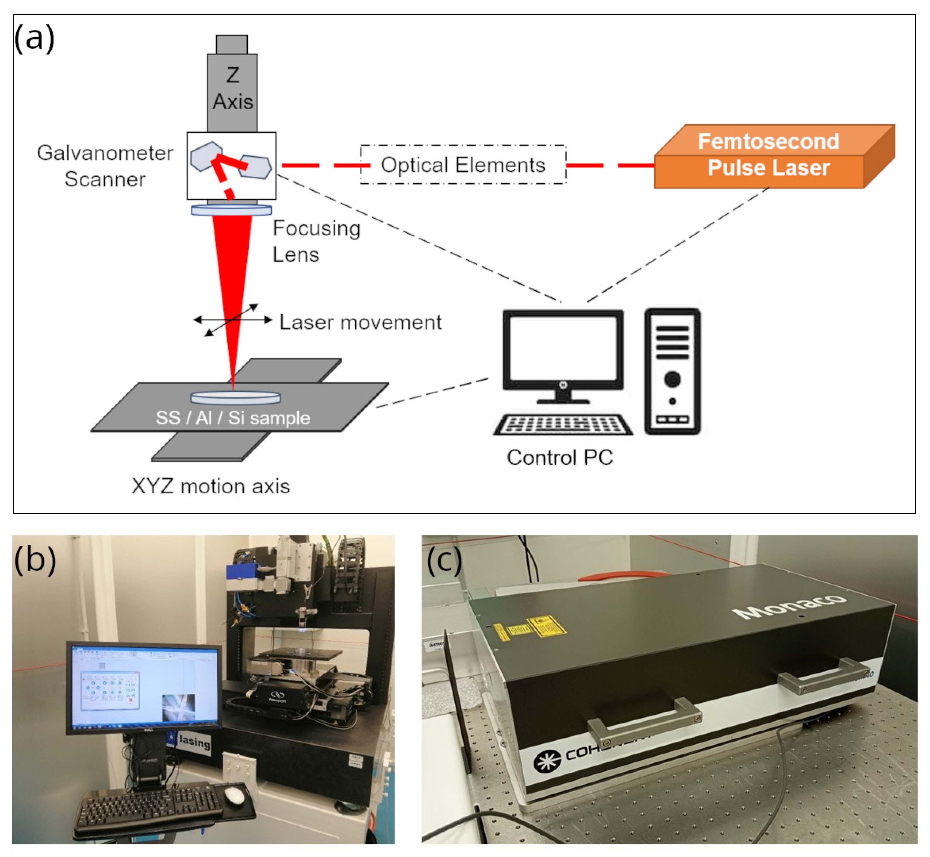
Experimental data were obtained using a femtosecond laser system integrated with a galvanometric beam scanning setup. A Monaco 1035-80-60 femtosecond laser source (by Coherent Corp., Santa Clara, CA, USA) was employed, delivering linearly polarized pulses at a central wavelength of 1035 nm and with a measured pulse width of approximately 280 fs. Figure 1 shows a schematic diagram of the experimental setup and images of the working station and laser device used at AIMEN facilities for the experimental characterization. The pulse repetition rate of this laser system can be tunable from single-shot operation up to 1 MHz using an acousto-optic modulator, and up to tens of MHz without pulse picking. The output beam exhibited a near-Gaussian spatial profile, with a beam diameter of approximately 2.8 mm in both transverse directions and a circularity of about 96%. Among the USP laser systems available at AIMEN facilities, this laser system was chosen as the most similar to the one used by the LS-Plume® simulator developed by Lasea [20].
The laser beam was guided through a galvanometer scanner and focused onto the sample surface using a telecentric fused-silica F-theta lens optimized for the 1030–1080 nm wavelength range. The lens had a nominal focal length of 160 mm, a maximum input beam diameter of 14 mm and a usable working area of 100 × 100 mm2. Due to the dynamic limitations of the galvanometric scanner, scanning speeds were kept below 1500 mm/s to ensure accurate beam positioning and to guarantee that the effective scanning velocity on the sample matched the programmed values.
Laser engraving tests were performed using a scanned-line machining strategy, producing straight channels of approximately 5 mm length. For each investigated material, i.e., SS 316, Si and Al, channels were fabricated using different combinations of pulse energy (between 10 and 50 uJ), repetition rate (between 10 and 200 kHz), scanning speed and number of passes (between 1 and 10), thus covering a broad range of peak fluence and pulse overlap conditions. Identical processing strategies and parameter ranges were applied to the three different materials to ensure consistency across experimental datasets.
The effective laser spot size on the material surface was experimentally determined by generating pulse-separated irradiations. This was achieved by appropriately adjusting the scanning speed and pulse repetition rate to minimize pulse overlap for each peak fluence condition. The resulting individual laser footprints were later analyzed to extract the beam diameter at focus, which was used for the calculation of fluence and overlap parameters.
The fabricated channels and laser footprints were characterized using a Sensofar Neox S confocal optical microscope (sourced by Sensofar Metrology, Terrassa, Spain). Measurements were performed in confocal scanning mode using a 50× objective, enabling high-resolution three-dimensional surface topography acquisition. From the measured profiles, the channel depth and the FWHM of the depth profile were extracted and used as output variables in the subsequent data analysis and ML models.

2.2. Computer Simulations

Computer simulations were used to extend experimental findings. For this purpose, a simulation model that solves the well-defined absorption law of energy and includes incubation effects, surface reflectivity and Gaussian beam diameter variations due to focal distance [21] was used to reproduce experimental ablation depths as a function of ablation energy, ablation threshold and radiation penetration depth, and was run through the LS-Plume® simulator developed by Lasea [20]. Thanks to it, we could simulate different surface topographies resulting from ultrafast laser ablation with different machining methods (scanned lines or areas, precession and percussion) with stainless steel 316L (SS 316), thus obtaining different ablation profiles for different laser settings. These laser settings correspond to input process parameters such as pulse energy, repetition rate, spot size at the focal point and scanning parameters such as speed, pitch between consecutive lines and incident angle. Similarly, material-specific parameters for SS 316 were used, including ablation threshold, laser penetration depth and refractive index.
The model expands on the classic logarithmic ablation law, where the ablation depth per pulse z depends on the material’s penetration depth δ and the ratio between the local applied laser fluence F and the material’s ablation threshold F t h :
z = δ ln F F t h .
Because the laser beam has a Gaussian intensity profile, the local fluence decreases exponentially at a radial distance r from the center of the beam, where F 0 is the peak fluence and ω 0 is the beam radius at 1 / e 2 :
F ( r ) = F 0 exp 2 r 2 w 0 2 .
To accurately predict dynamic, multi-pulse industrial operations (such as engraving lines or areas), the model integrates several critical interdependent phenomena:
  • Incubation: The material accumulates microscopic defects with N successive laser pulses, which increases its absorption coefficient and lowers the ablation threshold F t h ( N ) relative to the single-pulse threshold F t h ( 1 ) using an incubation coefficient:
    F t h ( N ) = F t h ( 1 ) · N S 1 ,
    where S stands for the incubation coefficient, which is an empirical parameter that depends on the strength of the incubation in the target material and is bound between 0 and 1.
  • Local Surface Angle and Reflectivity: As the laser carves into the material, the initial flat surface becomes a curved cavity. The local angle of incidence changes continuously, altering both the geometric area intercepting the beam and the material’s reflectivity R. The model dynamically recalculates the local absorbed fluence F a b s , N ( r ) based on the local wall slope angle θ ( r ) and Fresnel equations for specific light polarizations:
    F a b s , N ( r ) = F N ( r ) · ( 1 R ) · c o s θ ( r ) .
  • Beam Propagation: As the trench deepens by a distance z, the bottom moves away from the optical focal plane. The model integrates Gaussian beam propagation laws to adjust for the natural widening of the laser spot radius ω ( z ) based on the Rayleigh distance z R :
    ω ( z ) = ω 0 1 + z z r 2 .
By replacing pure radial symmetry with a 2D (x, y) numerical grid, the algorithm combines scanning speed v and pulse repetition rate P R R to determine the pulse distance interval δ x = v / P R R , calculating the exact spatial distribution of energy deposited during a scan.
The LS-Plume® simulator showed a good agreement between simulated and experimental results, in part thanks to the fact that thermal effects are not considered in the simulation model while experiments were also run under conditions where thermal contributions to laser ablation are minimal. This engineering tool successfully balances computational speed with physical accuracy by unifying incubation, Fresnel reflectivity, beam divergence, and scanning kinematics, and provides manufacturers with a reliable method to predict final part topography and optimize industrial laser processes for both time and energy efficiency. The model was validated using polished 316L stainless steel samples irradiated with a 1030 nm femtosecond laser (≈330 fs). The material’s intrinsic properties were determined to be F t h ( 1 ) = 0.1 J/ cm 2 , S = 0.8, and δ = 50 nm. The resulting micromachined topographies were mapped using a high-resolution confocal optical microscope, and the model perfectly predicted ablation depth and wall profiles for low to medium energy regimes, as well as the effects of shifting scanning speeds (from 50 to 450 mm/s). In multi-pass milling (17 to 33 passes), the simulated curves closely matched the real geometric slopes. A slight discrepancy appeared at 65 passes, where the real trench width was 8 µm narrower than predicted; the authors attribute this to debris accumulation on the edges and thermal swelling, which were excluded from the model’s simplified hypotheses. Finally, tests with a 15-degree tilted beam successfully demonstrated the model’s ability to predict asymmetrical profiles and negative wall conicities (97° angles).
The generated data relied on the scanned line machining strategy, where the ablation profile arises from the overlap of parallel engraved lines spaced evenly. To handle the large volume of data generated, it was saved in tabular format and processed with Python 3.

2.3. Machine Learning

ML is a branch of artificial intelligence that enables systems to learn patterns and make decisions or predictions from data. ML encompasses different techniques, depending on the problem to be solved and the data type. In this subsection, we introduce the different approaches used in the present work.

2.3.1. Neural Networks

In regression problems, neural networks (NNs) are ML models designed for predicting continuous numerical outputs from input data [22]. They consist of interconnected layers of neurons, where each neuron applies a mathematical operation to its inputs and passes the result through an activation function [23]. These layers are organized into an input layer (representing the input features), one or more hidden layers that capture complex patterns, and an output layer that generates the predicted target values. Thus, the general equation that represents a NN with n hidden layers can be expressed as follows:
y = f n W n f n 1 W n 1 f 0 W 0 x + b 0 + + b n 1 + b n ,
where x is the input vector, y is the output vector, n is the number of hidden layers, W i and b i are the weight matrices and biases, respectively, connecting layer i 1 to layer i and f j is the activation function for layer j, usually a ReLU, sigmoid, tanh or linear function.
Training a NN involves learning the W i and b i coefficients in such a way that the error between its predictions and the actual target values is minimized. This error is measured using a loss function, such as Mean Squared Error (MSE) or Mean Absolute Error (MAE), which quantifies how far the predictions are from the actual values. The learning process uses a method called Backpropagation algorithm to adjust these weights and biases by calculating the gradients of the loss function with respect to each parameter in the network and then using optimization algorithms, like Gradient Descent or Adam, to update the parameters iteratively [23].
Thanks to their flexible architecture and non-linear nature, NNs can model complex relationships in data and capture intricate patterns. Regularization techniques, such as dropout or L2 regularization, are often applied during training to prevent overfitting and improve generalization [23]. NNs have already showed their huge potential in industrial, financial or banking applications [24].

2.3.2. Transfer Learning

TL is a powerful ML approach that leverages the knowledge gained from a source domain to extend its applicability to a different domain [25]. TL, particularly through fine-tuning, has become a cornerstone of modern ML applications. It has facilitated breakthroughs in fields such as computer vision, natural language processing and medical diagnostics by enabling the reuse of robust pre-trained models [25]. By starting with a pre-trained model, TL allows to generate a new model valid in a different domain, thus being especially useful in scenarios with limited labeled data. This approach works by transferring the patterns learned in the original domain and derived from a large dataset to another domain, allowing models to generalize better to new tasks. Thus, this approach assumes that there are patterns which work in both domains, and just tries to learn the differences between the two domains.
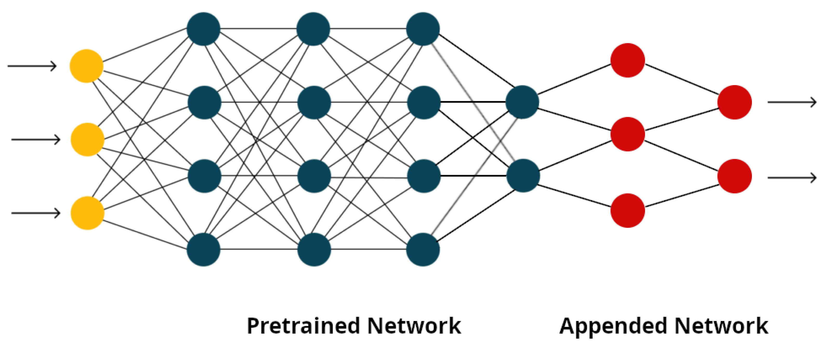
In this work, we propose two different approaches: the first one to learn and correct deviations in simulation data from experimental results, in which the source and target domains correspond to simulations and experiments, respectively, and the second one to transfer the patterns learned in SS 316 (source domain) to Si and Al, in which these different materials constitute the target domains. Specifically, a NN initially trained on SS 316 simulation data is fine-tuned to extend its applicability to SS 316, Si and Al experimental data. This is achieved through fine-tuning, a common TL technique in which a pre-trained model is adapted to a new task by updating part of its parameters. The fine-tuning technique involves taking a pre-trained NN and adapting it to the target task by updating its parameters. Typically, the first network’s layers remain unchanged, while the last layers are retrained or some extra layer is added to suit the new dataset in the new domain. This strategy is illustrated in Figure 2: yellow circles represent input features; dark blue nodes denote pre-trained layers kept frozen; and red nodes correspond to layers retrained or newly added for the target domain. Since the base model has already captured the fundamental relationships between input and target variables, the new layers focus on learning the deviations required for accurate predictions in the new domain.
From a physical perspective, the base network learns geometry- and energy-driven relationships inherent to the LST process that are largely material-independent. The TL stage then adjusts experiment- and material-dependent scaling factors associated with thermophysical and chemical properties. Usually, this new training is simpler and requires a significantly reduced amount of training data, making it particularly suitable for laser material processing, where experimental data acquisition is costly and time-consuming.
Additionally, this also results in lower training times, thus making this approach less computationally demanding. However, appended extra layers can be added either before or after the base layers, depending on the specific task and the architecture of the model. When they are added after the base layers, these new layers are trained to adapt the pre-trained features to the new task; while they can be added before the base layers if the input data for the new task have a different structure or require additional preprocessing.
In applying TL to capture deviations between simulated and experimental data, we used base models consisting of a NN with four input features and two target features, trained on simulation data for SS 316 (Section 3.1). We trained models with varying numbers of hidden layers and nodes per layer, considering both a multi-target configuration with two outputs in the same network and single-target configurations treated independently. Once these pre-trained networks were validated, their training parameters were frozen, and an additional layer was introduced. The hyperparameters of this new layer were then fine-tuned using experimental data to predict the targets in the new domain. Given the small size of the experimental dataset (20 data points for SS 316, 49 for Si and 46 for Al), training a complex NN from scratch would not have been feasible to capture all input–output patterns. However, with the TL approach, it became possible to adapt the base models trained on SS 316 simulation data by adding an extra hidden layer with only a few parameters to be fitted with experimental results. The achieved accurate adaptation with such a limited number of experimental samples was possible because while the base models could capture relationships inherent to the LST process, the new layers capture experiment- and material-specific corrections, thus showing a separation between shared physical behavior and setup- and material-specific corrections.
In our comprehensive hyperparameter search for the base and TL models, we systematically evaluated a wide range of NN architectures by tuning the number of hidden layers (from 1 to 4 in the base model, and 1 additional layer in the TL model), number of epochs (50–300), the number of units per layer (from 2 to 256 in the base model, and from 1 to 32 in the TL model) and activation functions (comparing ‘identity’, ‘relu’ and ‘sigmoid’ functions), while also rigorously testing several regularization strategies, including dropout (with rates from 0.0 to 0.25), batch normalization and L2 weight decay (with penalties from 1 × 10⁻⁵ to 0.0).

2.3.3. Explainable Artificial Intelligence

xAI encompasses a set of techniques designed to make the decisions and predictions of complex ML models transparent and interpretable to humans. In this work, we used SHAP (SHapley Additive exPlanations) values to quantify input feature importance as derived according to cooperative game theory. SHAP conceptualizes the prediction task as a cooperative game where individual features act as players, and the model’s prediction constitutes the total payout [26].
To compute the exact contribution of a specific feature i, the methodology evaluates the change in the model’s prediction when feature i is included versus when it is excluded, averaged across all possible subsets of remaining features. Mathematically, the Shapley value ϕ i for feature i is defined as:
ϕ i = S M { i } | S | ! ( | M | | S | 1 ) ! | M | ! f x ( S { i } ) f x ( S ) ,
where M is the total set of features, S is a subset of features excluding i, and f x ( S ) is the conditional expectation of the model outcome given the features in S.
Because neural networks exhibit highly non-linear decision boundaries, computing exact Shapley values is computationally intractable. Therefore, we utilize the KernelExplainer, a model-agnostic local explanation method that uses weighted linear regression to approximate these values, by observing local shifts in predictions.
For any individual prediction, a feature’s SHAP value represents its localized force, indicating the magnitude and direction (positive or negative push). In this work, we visualize the results using SHAP summary plots. These plots allow us to interpret the directional impact of features, demonstrating whether high or low underlying values of a specific physical feature correlate with an increase or decrease in the network’s predictive output.


3. Results

3.1. Data Analysis and Preprocessing

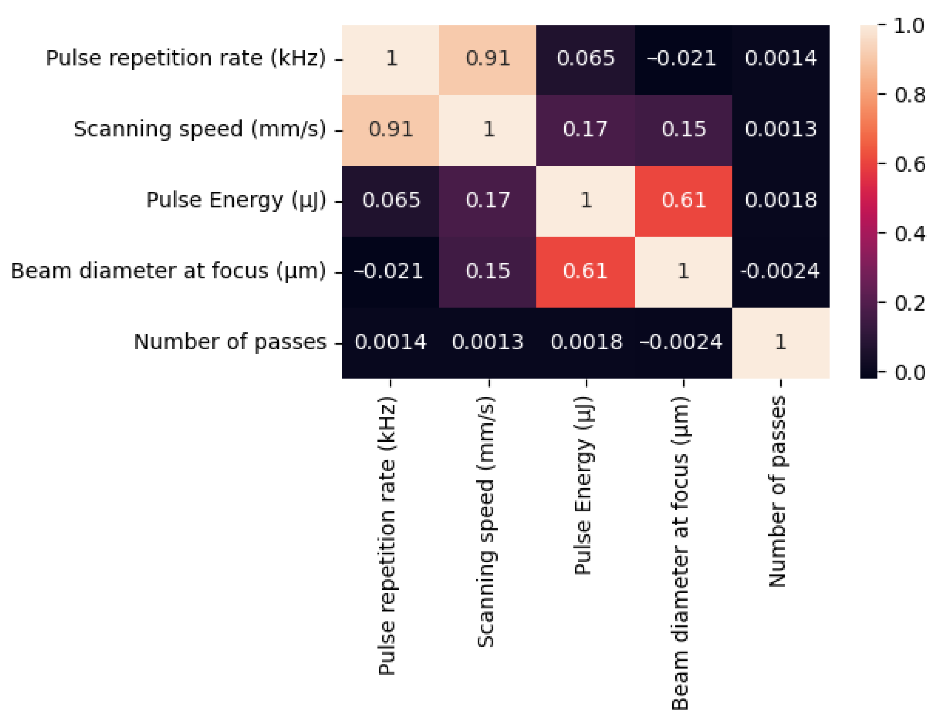
LST is a complex process that brings about a strong effect of process parameters on the resulting surface shape. Usually, the critical input parameters are the pulse repetition rate, scanning speed, pulse energy, beam diameter at focus and number of passes, which can be considered as input features. On the other hand, the resulting surface textures can be described by the depth of the material removed by the laser beam and its full width at half maximum (FWHM) depth, which will be considered as targets in our NNs. These input features are critical properties in LST, as they collectively influence the precision, uniformity and efficiency of the process, and the two output targets are the most representative properties of the groove. The pulse repetition rate determines the frequency of laser pulses, affecting energy overlap and heat accumulation, while the scanning speed controls the laser’s interaction time with the material, and slower speeds enable deeper ablation. The pulse energy determines the energy received on the surface and has an impact on the material removal rate, and the beam diameter at focus defines the interaction area. Figure 3 shows the correlation matrix among features and targets with the corresponding Pearson correlation coefficient with simulation data for SS 316. For each pair of variables, the Pearson correlation coefficient wass computed as the ratio between their covariance and the product of their standard deviations [27]. Zero values indicate no linear correlation, while +1 and −1 values indicate a perfect positive and negative linear correlation, respectively, between two variables.
However, since these five input features are not independent, as shown in Figure 3, the input variable space was reduced to four variables: number of passes, peak fluence, overlap and beam diameter at focus. Due to the strong correlation between pulse repetition rate and scanning speed, these two variables are no longer considered as input features and are replaced by the overlap, which is defined as follows:
Overlap [ % ] = 1 Scanning Speed Beam Diameter × Pulse Repetition Rate .
Additionally, the pulse energy, which is not an independent feature either, was replaced by the peak fluence, defined as follows:
Peak Fluence = 2 × Pulse Energy π × Beam Diameter / 2 2 .
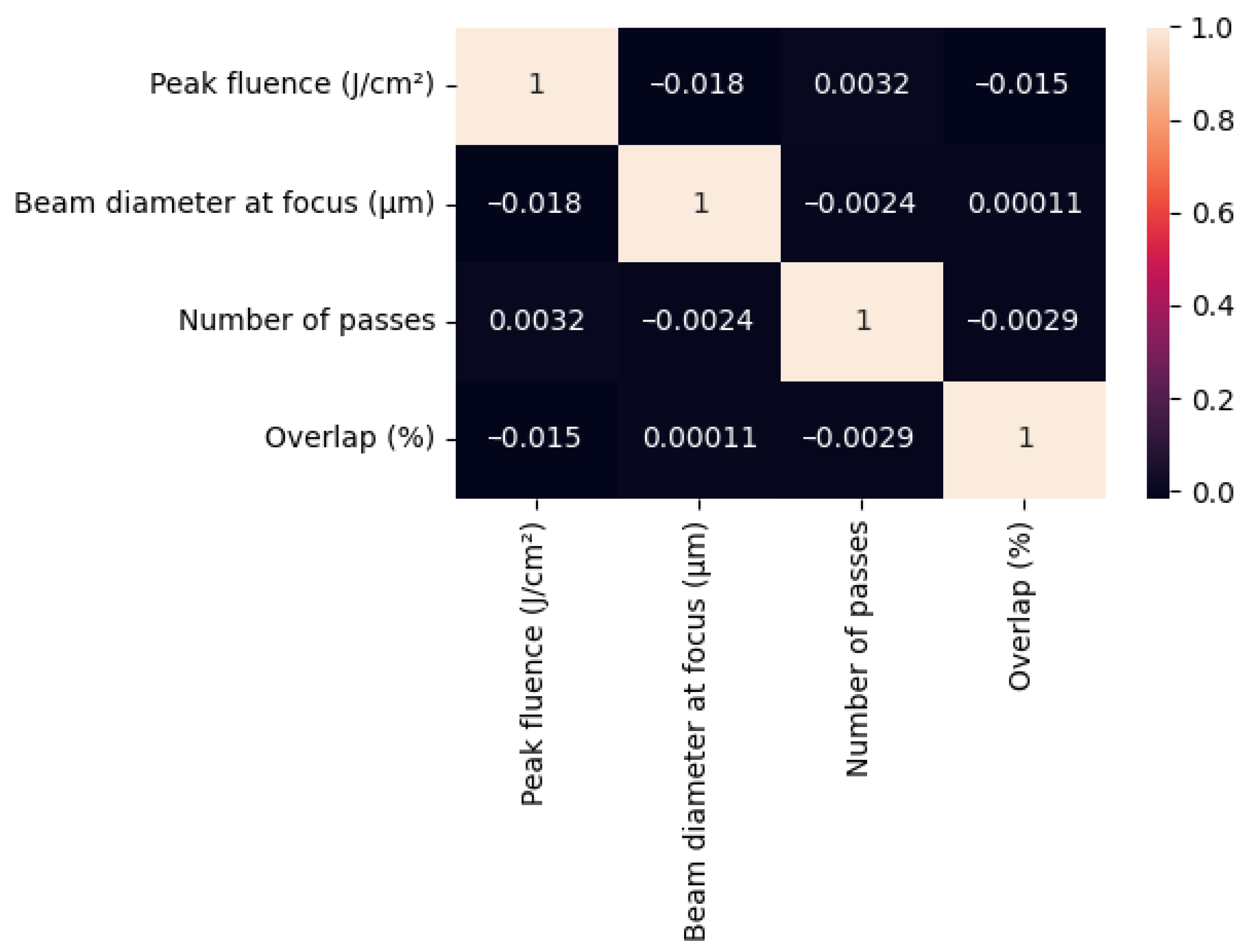
As observed in Figure 4, the new input features can be considered as independent, thus allowing generating a complex model that determines the pattern between the output features as a combination of all new input features.
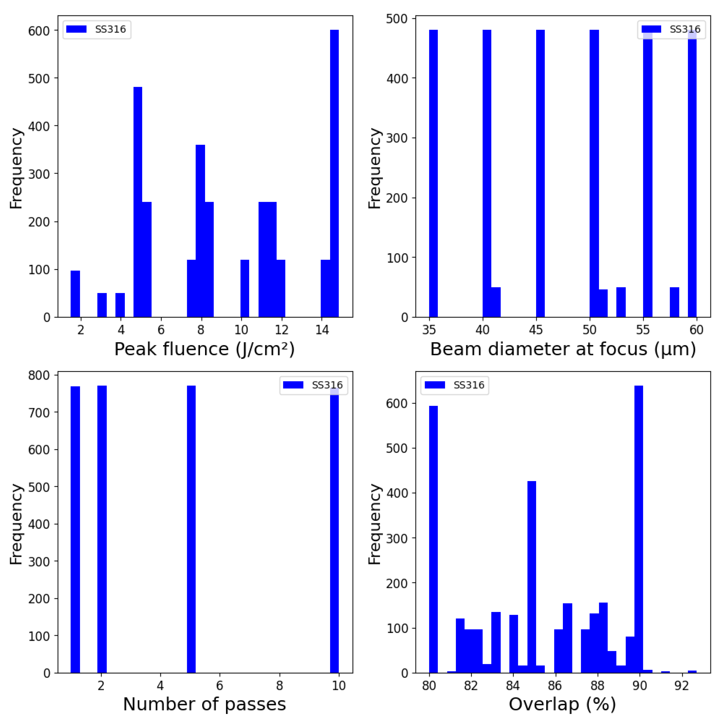
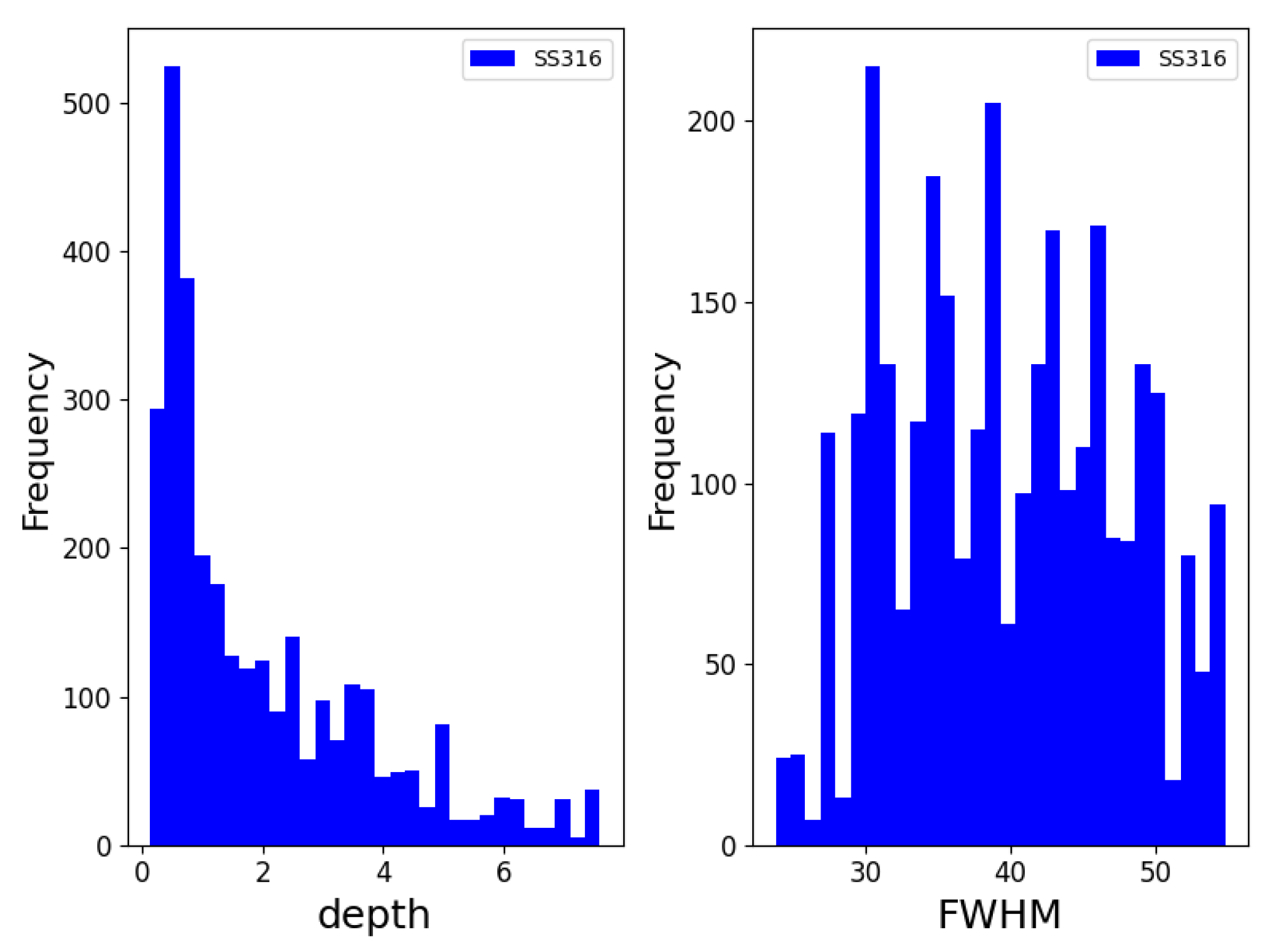
In this work, we propose a NN to capture the relationship between these four input features and the two targets. This network is trained with SS 316 simulation data, and will constitute our base model. Then, we will train different models by extending this base model with TL to learn deviations from experimental results and extrapolate this learning to different materials: Al and Si. The details of these networks and their training and performance are described in the following subsections. The distribution of the input and output simulation values can be seen in Figure 5 and Figure 6, respectively, showing that the variable space is well covered. Since the output values for depth are concentrated at lower values, the natural logarithm of one plus the value is used as output feature instead.
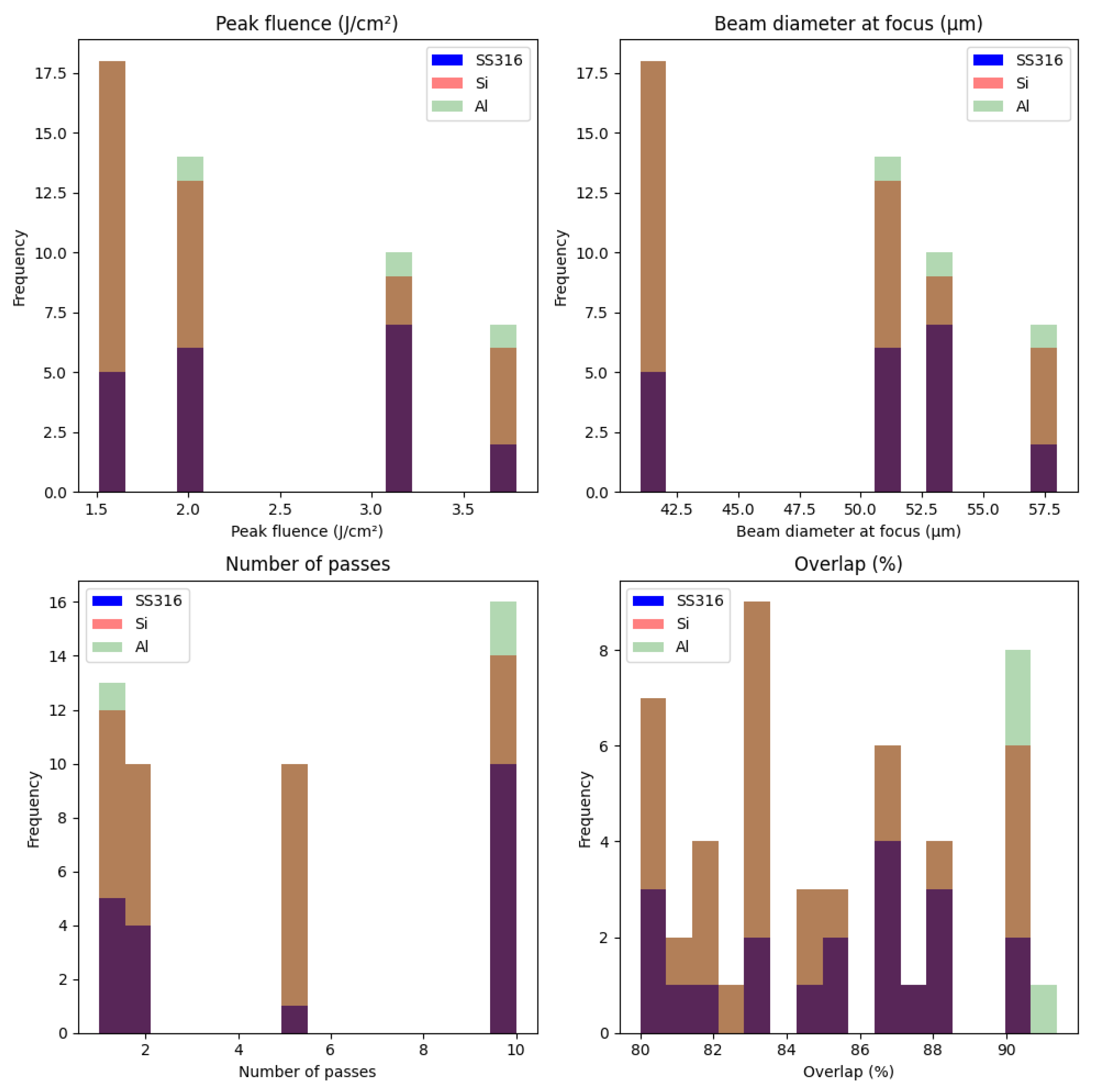
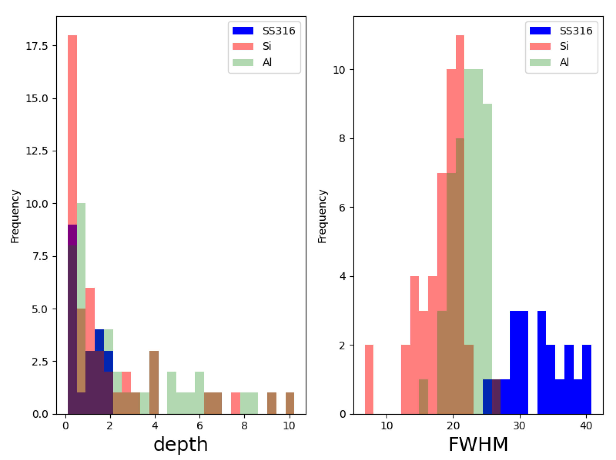
Similarly, Figure 7 and Figure 8 show the distribution of the input and output experimental values, respectively, corresponding to 20 data points for SS 316, 49 for Si and 46 for Al. Here it is important to highlight that experimental depths are usually lower than the observed in simulations. Additionally, experiments in SS 316 also present smaller depths and larger FWHM values than the observed in Al and Si. The goal of this work was to train TL models to learn this different material-dependent behaviour.

3.2. Base Model: Stainless Steel 316

NNs were used to describe the impact of the four process parameters described above (i.e., number of passes, peak fluence, overlap and beam diameter at focus on surface texture) for each output target: depth and FWHM. These NNs were trained with simulation data generated by the LS-Plume® simulator for SS 316. 3075 simulations were performed, and the dataset was split into training and test datasets, with the 15% used for testing. The input values were scaled by removing their mean value and then scaling to unit variance, and the natural logarithm of one plus the output values was applied to the targets to generate a more uniform distribution.
Different NNs were trained to minimize the error in the test dataset. After exploring different number of nodes in two hidden layers and different activation functions, higher accuracy was observed when the two output targets were predicted independently in separate NNs. The lowest errors were obtained with two hidden layers formed by 128 and 24 nodes and under the linear and activation functions respectively for depth prediction, and by 96 and 16 nodes for FWHM (see Table 1). The NN coefficients were obtained with the Adam optimizer.
The performance of the base and TL models was evaluated using the MAE metric on the experimental dataset. The selected base models (BM1 and BM2), characterized in Table 1, were first evaluated on SS 316 simulation data. The MAEs in the test datasets were 0.0075 and 0.1750 µm for depth and FWHM, respectively, which corresponds to percentage errors below 1%, thus indicating a great accuracy and no overfitting. These pre-trained models were then used to train TL models, as described in the following subsections.

3.3. Transfer Learning from Simulation Data to Experimental Data in SS 316

As we can see in Table 2 for SS 316, when the base models BM 1 and BM 2 , trained on simulation data, are evaluated on experimental data, their performance drops. This is caused by the assumptions made on the simulation model and the intrinsic noise present in experimental data, and not because of bad performance of the NN. Therefore, in order to reduce the deviations from simulations to experiments, we used these two pre-trained NNs to fine-tune new TL models for prediction on SS 316 experimental data ( TL 1 and TL 2 , for depth and FWHM, respectively), resulting in the architectures and associated errors reported in Table 1 and Table 2 for SS 316. When the TL approach was applied to experimental data in SS 316, the additional layers captured the deviations of the simulations with respect to the experiments. The error of the TL models on the experimental dataset is higher than that of the base models on the simulation data, which is expected considering that the TL models were trained with limited data and must account for the deviations between simulations and experiments. However, as shown in Table 2, the TL models overperform the base models when evaluated on the experimental dataset. This demonstrates their ability to capture systematic patterns in the deviations and correct the base predictions accordingly.
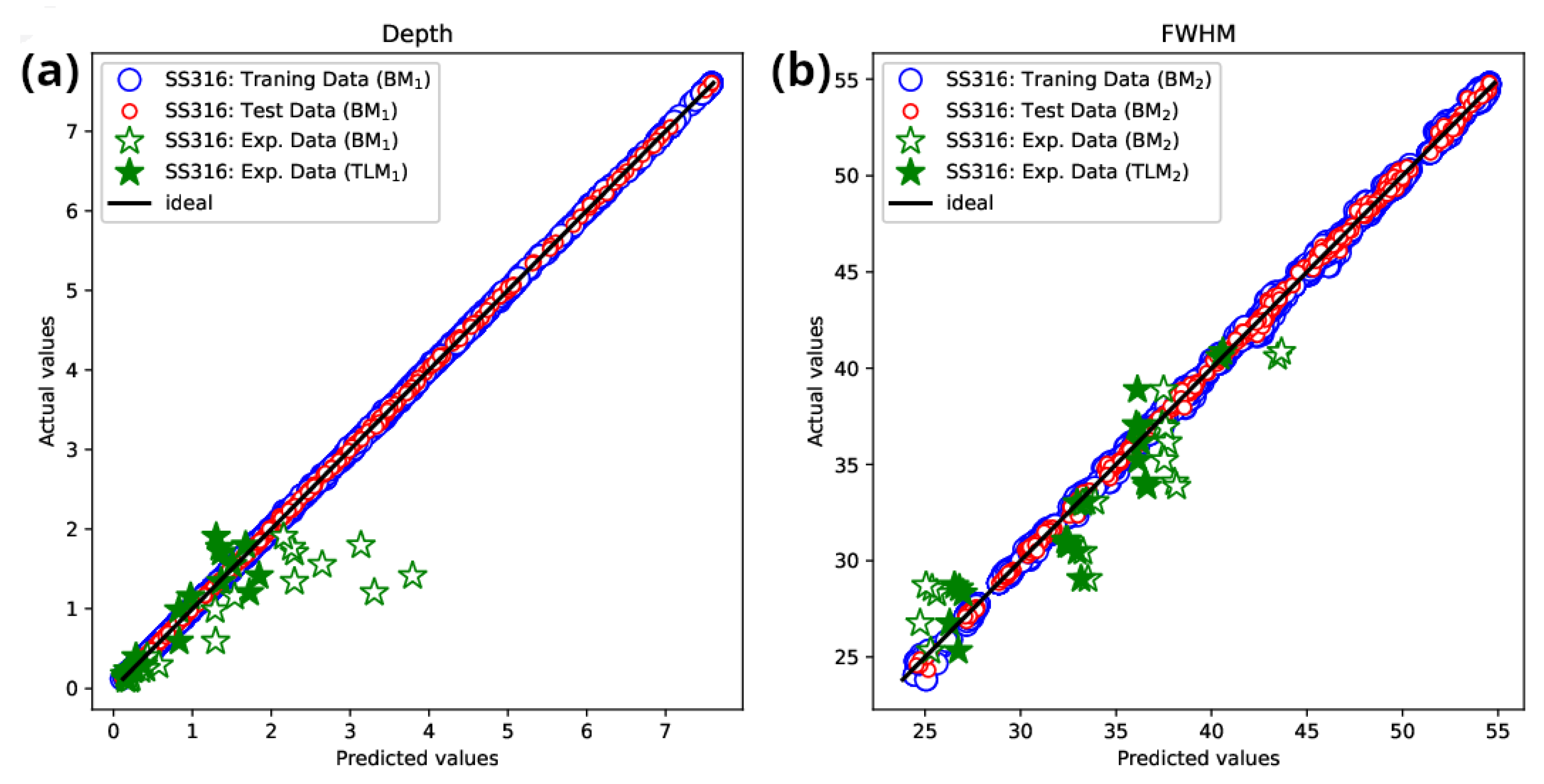
Figure 9 illustrates these results by showing the deviation of the predictions of the base and TL models from the actual values. The empty red circles indicate that the base models provide highly accurate predictions when evaluated on simulated data for SS 316, with low MAE values as reported in Table 1. This confirms that the NNs successfully captured the relationships between input features and targets in the simulation dataset, with no overfitting. However, when evaluated on SS 316 experimental data (empty stars), the MAE values of the base model predictions increased, as reported in Table 2, revealing an intrinsic deviation between simulation and experiment that is not caused by the NN itself. To address this, the TL 1 and TL 2 models were trained with only 20 experimental samples, achieving a considerable reduction in errors (filled stars), as also shown in Table 2. These results are of particular industrial interest, as they highlight that the combination of ML and computer simulations, enhanced through TL approaches, provides a powerful framework for automating USPL experiments even under data-scarce conditions.

3.4. Transfer Learning to Other Materials

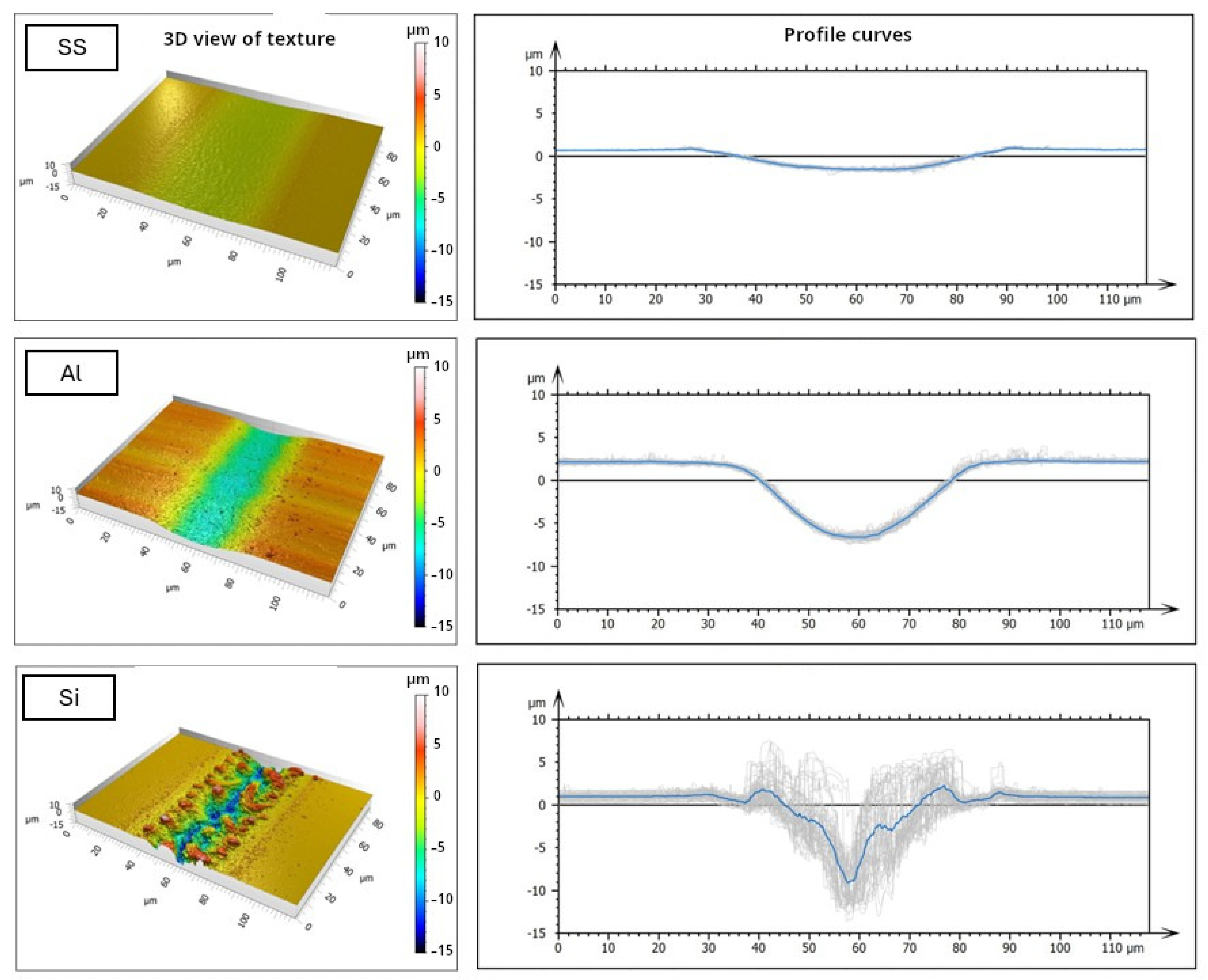
Given the great performance of the base models trained on SS 316 simulation data, we extended their use to Si and Al through TL approaches. As observed in Figure 10, the chemical composition of the sample determines plays a critical role in the ablation profile properties, thus showing that the findings obtained for SS 316 cannot be directly applied to Si and Al and proving the need for an extended TL framework. For this purpose, the new TL NN layers captured both the effect of the different materials on the output targets and the systematic deviations between simulated and experimental data. The resulting models, finetuned with only 49 samples for Si and 46 for Al, are described in Table 1 and their prediction performance is reported in Table 2.
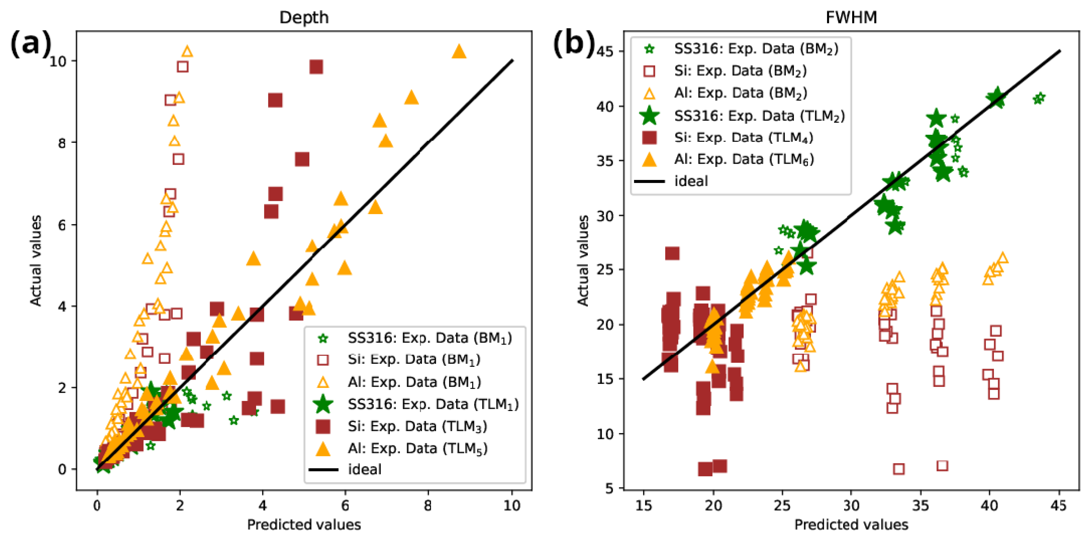
The comparison between base and TL models is presented in Figure 11. Empty symbols stand for the predictions of the base models trained on SS 316 simulation data, while filled symbols correspond to the TL models trained on the experimental data for each respective material. Although the deviations from the ideal behaviour are larger for Si and Al than those observed for SS 316, the results remain robust. This demonstrates that the TL models not only learned the impact of different materials on the output targets, but also the patterns of deviations between simulation and experimental data.
As expected, the base models trained on SS 316 simulation data cannot directly predict the targets in Al and Si, due to the different behaviour of these chemical species. However, after training the TL models, the MAE errors were reduced considerably, as shown in Table 2. These errors are now comparable to those observed for SS 316 experimental data, confirming that the TL approach was successfully and accurate enough for potential industrial application. In the case of Si, the errors are larger, mainly because the FWHM values are lower than those typically obtained for SS 316 under the same input conditions. By contrast, for Al, the errors in predicting FWHM values are even smaller than those observed for SS 316.
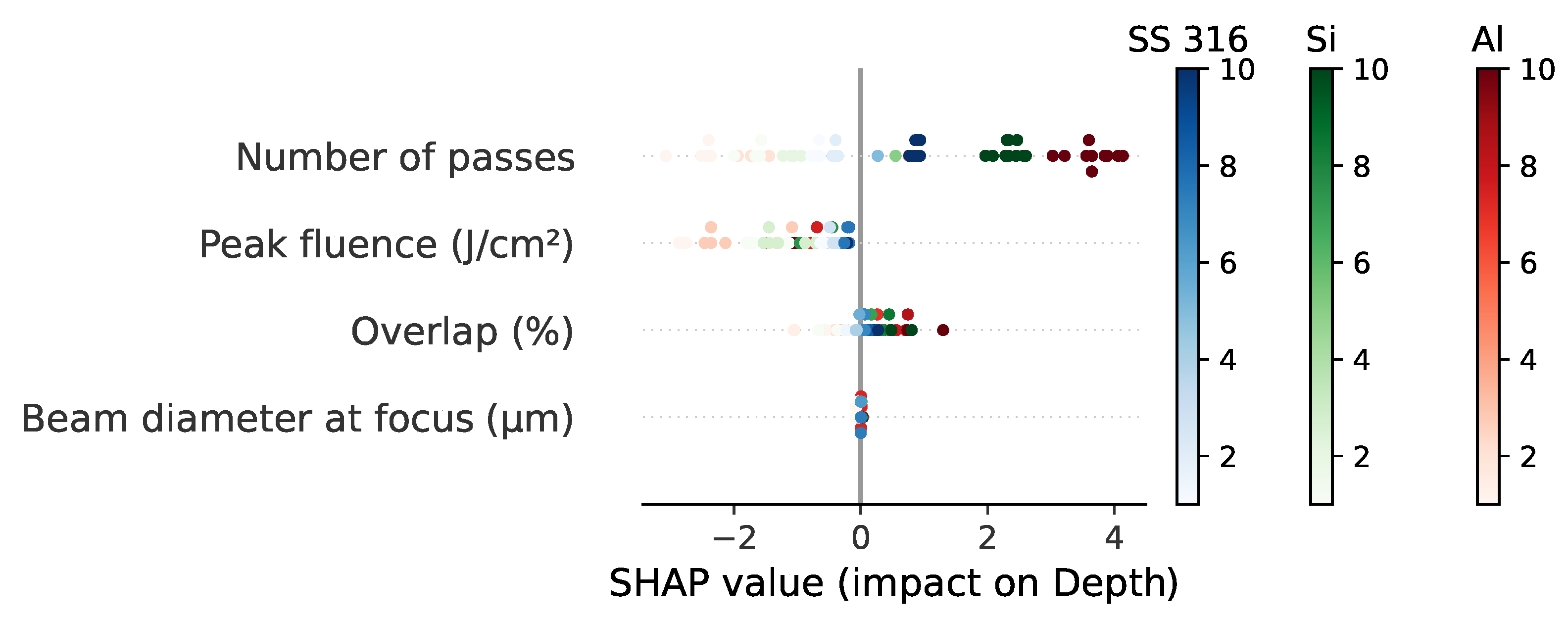
We also compared the effect of the input features on the targets for the different materials by computing SHAP values. Figure 12 shows the SHAP values computed from local weighted linear regression [26] for depth predictions. In this figure, we can see that the number of passes and peak fluence are the dominant factors controlling depth in the laser processing model, with higher energy levels and additional passes significantly increasing penetration depth. On the other hand, overlap percentage and beam diameter show lower impact on depth outcomes. Additionally, we also see that the number of passes has a larger impact on Si and Al than on SS 316. This different behavior is associated with their different material properties. Due to its lower thermal conductivity and higher reflectivity, Si requires higher laser energy densities to achieve melting or ablation, often resulting in rougher textures, while SS 316 undergoes smoother behaviour. The input process parameters may have a more significant impact on SS 316 because its response is more sensitive to thermal gradients and cooling rates, which are directly influenced by these parameters. From a practical standpoint, these results indicate that SS 316 exhibits a more robust and predictable depth response to parameter variations, whereas Si and Al are more sensitive to energy accumulation through multiple passes, requiring tighter process control to achieve consistent penetration depths.
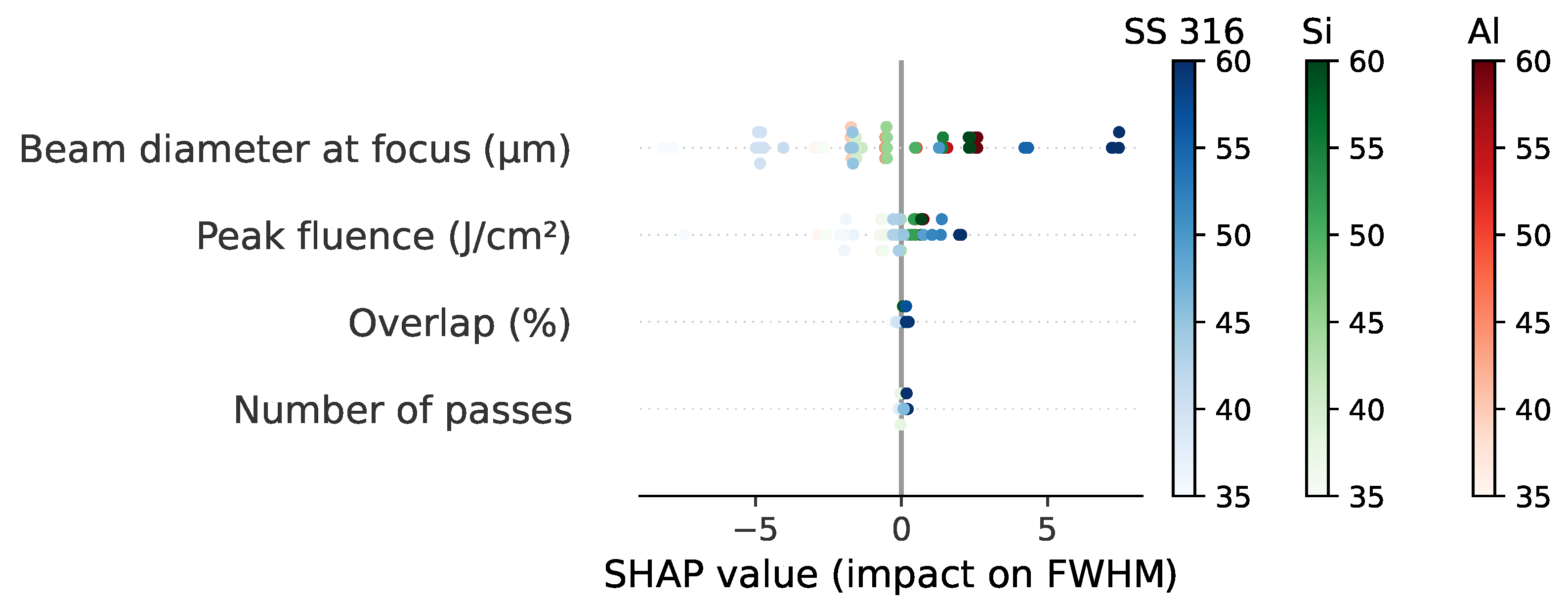
Figure 13 shows the SHAP analysis for FWHM predictions. In this case, beam diameter emerges as the most influential parameter for FWHM across all materials, with higher fluence levels generally increasing FWHM, particularly in SS 316 and Si. Peak fluence shows moderate influence, especially in Al, where larger diameters correlate with wider features. The material-specific responses reveal that Al and Si behave similarly, with both being highly sensitive to fluence variations. The number of passes and overlap percentage have relatively minor impacts on FWHM compared to fluence and beam diameter. This indicates that controlling feature width primarily requires careful management of beam diameter, with secondary attention to peak fluence, while the material-specific differences highlight the need for tailored parameter optimization for each material. In an industrial context, this implies that beam diameter acts as the primary lever for dimensional control across all materials, while fluence-driven sensitivity is more pronounced in Al and Si, making SS 316 comparatively more tolerant to energy fluctuations during processing.

4. Conclusions

In this work, we showed how the application of TL approaches to simulation and experimental data can help predict the behaviour of different materials during LST process using USPL. We used an improved simulation dataset working with single-beam and individual groove ablation profiles, generated using the LS-PLUME® simulator by Lasea. This computational dataset was then complemented with experimental studies to capture the deviations from simulation to experiments and then generate an experimental dataset on Si and Al to apply TL approaches.
Summarizing this study, the main contributions of this work are threefold:
  • TL has shown to be a promising strategy for bridging the simulation-to-experiment gap under data-scarce conditions, thus ensuring simulation results can be directly applied to solve real-world industrial problems. Our approach successfully adapted the model to absorb systematic deviations between simulations and experiments by enabling simulation-trained models to be reliably transferred to real experimental conditions with SS 316.
  • Thanks to TL approaches, the knowledge learned on SS 316 can be successfully transferred to Al and Si, chemically and thermophysically distinct materials, using only a very limited amount of experimental data. While the database for SS 316 simulations data consisted of 3075 simulations, the TL models were finetuned with only 49 and 46 experimental data points for Si and Al, respectively.
  • SHAP analysis provides physically meaningful insight into the learned representations, showing that the number of passes is the most relevant feature during LST. Thanks to this knowledge learned from xAI analysis, we can understand how the LST process works and then optimize it to generate surfaces with tailored properties, which is of high interest in industrial applications.

Author Contributions

Conceptualization, S.M.-L. and B.B.-F.; methodology, J.F.T., M.G.-V., T.D. and C.P.; software, J.F.T.; validation, B.B.-F. and V.A.-P.; formal analysis, B.B.-F. and V.A.-P.; investigation, S.V., P.R. and D.B.; resources, S.V., D.B.,S.M.-L.; data curation, J.F.T. and B.B.-F.; writing—original draft preparation, J.F.T.; writing—review and editing, B.B.-F. and V.A.-P.; visualization, J.F.T.; supervision, S.V., P.R., D.B. and S.M.-L.; project administration, D.B., P.R. and S.M.-L.; funding acquisition, D.B., P.R. and S.M.-L. All authors have read and agreed to the published version of the manuscript.

Funding

This research was funded by the European Union’s Horizon Europe research and innovation programme under grant agreement No. 101058409 (OPERATIC).

Data Availability Statement

The data presented in this study are available on request from the corresponding author.

Conflicts of Interest

The authors declare no conflict of interest. The funders had no role in the design of the study; in the collection, analyses, or interpretation of data; in the writing of the manuscript; or in the decision to publish the results. Authors Céline Petit and David Bruneel were employed by the company LASEA. The remaining authors declare that the research was conducted in the absence of any commercial or financial relationships that could be construed as a potential conflict of interest.

References

  1. Kobayashi, T. Ultrashort Pulse Lasers and Ultrafast Phenomena, 1st ed.; CRC Press: Boca Raton, FL, USA, 2023. [Google Scholar] [CrossRef]
  2. Nolte, S.; Schrempel, F.; Dausinger, F. (Eds.) Ultrashort Pulse Laser Technology: Laser Sources and Applications; Springer Series in Optical Sciences; Springer International Publishing: Cham, Switzerland, 2016; Volume 195. [Google Scholar] [CrossRef]
  3. Nishizawa, N. Ultrashort pulse fiber lasers and their applications. Jpn. J. Appl. Phys. 2014, 53, 090101. [Google Scholar] [CrossRef]
  4. Blanco-Filgueira, B.; Delgado, T.; Gregores Coto, A.; Petit, C.; Bruneel, D.; Romero, P.; Muiños-Landin, S. Synthetic Data for AI-Powered Ultrafast Laser Based Micro-structuring Method Description. In Proceedings of the Advances in Artificial Intelligence in Manufacturing II. ESAIM 2024; Lecture Notes in Mechanical Engineering; Springer: Cham, Switzerland, 2025. [Google Scholar] [CrossRef]
  5. Ding, Y.; Jiang, X.; Wang, C.; Jia, X.; Liu, L.; Han, W.; Gai, Z.; Wang, S.; Lin, N.; Wan, D.; et al. Femtosecond Laser Rapid Customization of High-Performance Anti-Reflection Windows. Opto-Electron. Sci. 2026, 5, 260004. [Google Scholar] [CrossRef]
  6. Schille, J.; Schneider, L.; Streek, A.; Kloetzer, S.; Loeschner, U. High-throughput machining using a high-average power ultrashort pulse laser and high-speed polygon scanner. Opt. Eng. 2016, 55, 096109. [Google Scholar] [CrossRef]
  7. Moles, L.; Llavori, I.; Aginagalde, A.; Echegaray, G.; Bruneel, D.; Boto, F.; Zabala, A. On the Use of Machine Learning for Predicting Femtosecond Laser Grooves in Tribological Applications. Tribol. Int. 2024, 200, 110067. [Google Scholar] [CrossRef]
  8. Wang, L.; Gu, Y.; Tian, X.; Wang, J.; Jia, Y.; Xu, J.; Zhang, Z.; Liu, S.; Liu, S. Machine Learning-Assisted Optimization of Femtosecond Laser-Induced Superhydrophobic Microstructure Processing. Photonics 2025, 12, 530. [Google Scholar] [CrossRef]
  9. Rubenchik, A.; Feit, M.; Perry, M.; Larsen, J. Numerical simulation of ultra-short laser pulse energy deposition and bulk transport for material processing. Appl. Surf. Sci. 1998, 127–129, 193–198. [Google Scholar] [CrossRef]
  10. Savriama, G.; Semmar, N. Numerical Simulation of Laser Processing Materials: An Engineering Approach. In Modeling and Simulation in Engineering Sciences; Akbar, N.S., Beg, O.A., Eds.; InTech: Amsterdam, The Netherlands, 2016. [Google Scholar] [CrossRef] [PubMed][Green Version]
  11. Guo, J.; Ji, P.; Jiang, L.; Lin, G.; Meng, Y. Femtosecond laser sintering Al nanoparticles: A multiscale investigation of combined molecular dynamics simulation and two-temperature model. Powder Technol. 2022, 407, 117682. [Google Scholar] [CrossRef]
  12. Peng, L.; Li, M.; Wang, P.; Li, X.; Zhang, Y.; He, M.; Zhou, C.; Zhang, H.; Chen, S. Numerical simulation and investigation of ultra-short pulse laser ablation on Ti6Al4V and stainless steel. AIP Adv. 2023, 13, 065018. [Google Scholar] [CrossRef]
  13. Florian, T.; Buttazzoni, M.; Zenz, C.; Otto, A. Ultra-short pulse laser ablation of metals: A comprehensive 3D simulation perspective enlightening novel process insights. Procedia CIRP 2024, 124, 602–607. [Google Scholar] [CrossRef]
  14. Mrudul, M.S.; Oppeneer, P.M. Ab initio investigation of laser-induced ultrafast demagnetization of L 1 0 FePt: Intensity dependence and importance of electron coherence. Phys. Rev. B 2024, 109, 144418. [Google Scholar] [CrossRef]
  15. Shimahara, K.; Tani, S.; Sakurai, H.; Kobayashi, Y. A deep learning-based predictive simulator for the optimization of ultrashort pulse laser drilling. Commun. Eng. 2023, 2, 1. [Google Scholar] [CrossRef]
  16. Ji, X.; Chen, R.; Lu, C.; Zhou, J.; Zhang, M.; Zhang, T.; Yu, H.; Yin, Y.; Shi, P.; Zhang, W. Recent advances in machine learning for defects detection and prediction in laser cladding process. Next Mater. 2025, 7, 100404. [Google Scholar] [CrossRef]
  17. Zahavy, T.; Dikopoltsev, A.; Moss, D.; Haham, G.I.; Cohen, O.; Mannor, S.; Segev, M. Deep learning reconstruction of ultrashort pulses. Optica 2018, 5, 666. [Google Scholar] [CrossRef]
  18. Hoffmann, N.; Schmidt, J.; Botti, S.; Marques, M.A.L. Transfer learning on large datasets for the accurate prediction of material properties. arXiv 2023, arXiv:2303.03000. [Google Scholar] [CrossRef]
  19. Chen, Y.; Ding, X. Research on cross-Project software defect prediction based on transfer learning. In Proceedings of the AIP Conference Proceedings, Xi’an City, China; AIP Publishing LLC: Melville, NY, USA, 2018; p. 040083. [Google Scholar] [CrossRef]
  20. LASEA: Homepage-ls-Plume. Available online: https://portal.lasea.com (accessed on 1 July 2026).
  21. Bruneel, D.; Cangueiro, L.; Reed, C.; Braunschweig, R.; Martin, P.E.; Ramos-de Campos, J.A.; Kupisiewicz, A. Optimization of the micromachining process by the simulation of ultrafast laser ablated profiles on metals for different applications. In Proceedings of the ICALEO 2018: 37th International Congress on Applications of Lasers & Electro-Optics; Laser Institute of America: Orlando, FL, USA, 2018; p. M602. [Google Scholar] [CrossRef]
  22. McCulloch, W.S.; Pitts, W. A logical calculus of the ideas immanent in nervous activity. Bull. Math. Biophys. 1943, 5, 115–133. [Google Scholar] [CrossRef]
  23. Bishop, C.M. Neural Networks for Pattern Recognition; Clarendon Press: Oxford, UK, 1995. [Google Scholar]
  24. Dreyfus, G. (Ed.) Neural Networks: Methodology and Applications; Springer: Berlin/Heidelberg, Germany, 2005. [Google Scholar] [CrossRef]
  25. Hosna, A.; Merry, E.; Gyalmo, J.; Alom, Z.; Aung, Z.; Azim, M.A. Transfer learning: A friendly introduction. J. Big Data 2022, 9, 102. [Google Scholar] [CrossRef] [PubMed]
  26. Lundberg, S.; Lee, S.I. A Unified Approach to Interpreting Model Predictions. arXiv 2017, arXiv:1705.07874. [Google Scholar] [CrossRef]
  27. Freeman, D.; Pisani, R.; Purves, R. Statistics, 4th ed.; W. W. Norton & Company: New York, NY, USA, 2007. [Google Scholar]
Figure 1. (a) Schematic diagram of the experimental setup. Working station (b) and Monaco laser device (c) used at AIMEN facilities for the experimental work.
Jmmp 10 00244 g001
Figure 2. Schematic representation of a NN used for TL. The three yellow circles represent three input nodes (or features), the dark blue circles represent the nodes in the hidden layers trained in the original domain, and the red circles stand for nodes trained whose connections were trained with data from the new domain.
Jmmp 10 00244 g002
Figure 3. Correlation matrix of provisional input features and output targets computed with simulation data for stainless steel 316.
Jmmp 10 00244 g003
Figure 4. Correlation matrix of final input features computed with simulation data for SS 316.
Jmmp 10 00244 g004
Figure 5. Distribution of input features used to train and test the base model with simulation results for SS 316.
Jmmp 10 00244 g005
Figure 6. Distribution of output features used to train and test the base model with simulation results for SS 316.
Jmmp 10 00244 g006
Figure 7. Distribution of input features used to train and test TL models with experimental values for different materials. The histograms are plotted with semi-transparency to show overlapping distributions. Distinct intermediate colors (e.g., purple and brown) represent the visual overlap of the primary material distributions (SS 316, Si, and Al) and do not indicate separate data series.
Jmmp 10 00244 g007
Figure 8. Distribution of output features used to train and test TL models with experimental values for different materials.The histograms are plotted with semi-transparency to show overlapping distributions. Distinct intermediate colors (e.g., purple and brown) represent the visual overlap of the primary material distributions (SS 316, Si, and Al) and do not indicate separate data series.
Jmmp 10 00244 g008
Figure 9. Prediction error for depth (a) and FWHM (b) for SS 316 given by base and TL models listed in Table 1.
Jmmp 10 00244 g009
Figure 10. 3D view (LHS) and profile (RHS) of the lines performed with identical process parameters for SS 316, Al and Si. In the 2D profiles (RHS), grey lines represent the many profiles measured, while the blue line represents their mean value.
Jmmp 10 00244 g010
Figure 11. Prediction error for depth (a) and FWHM (b) for SS 316, Al and Si given by the base and TL models listed in Table 2 when evaluated on experimental data.
Jmmp 10 00244 g011
Figure 12. SHAP values computed for SS 316, Al and Si for depth. The intensity of colors represent how large or small the target values are for each material.
Jmmp 10 00244 g012
Figure 13. SHAP values computed for SS 316, Al and Si for FWHM. The intensity of colors represent how large or small the target values are for each material.
Jmmp 10 00244 g013
Table 1. Model name, training and test source, architecture, and MAE of the predictions of base and TL models (BM and TLM, respectively).
MaterialTargetModel NameSourceArchitectureMAE [µm]
SS 316depth BM 1 Simulations4 input features ×
128 nodes × 24 nodes
× 1 target feature
0.0075
TLM 1 Experiments BM 1 + 16 × 10.1750
FWHM BM 2 Simulations4 × 96 × 16 × 10.1259
TLM 2 Experiments BM 2 + 5 × 11.4104
Aldepth TLM 3 Experiments BM 1 + 16 × 10.3706
FWHM TLM 4 Experiments BM 2 + 1 × 10.7395
Sidepth TLM 5 Experiments BM 1 + 12 × 10.7241
FWHM TLM 6 Experiments BM 2 + 4 × 12.3486
Table 2. Prediction metric of base and TL models described in Table 1 when evaluated on experimental data.
MaterialDepthFWHM
Base ModelTL ApproachBase ModelTL Approach
NameMAENameMAENameMAENameMAE
SS 316 BM 1 0.5720 TLM 1 0.1750 BM 2 2.1675 TLM 2 1.4104
Al1.5305 TLM 3 0.370610.3477 TLM 4 0.7395
Si0.9213 TLM 5 0.724113.9444 TLM 6 2.3486
Disclaimer/Publisher’s Note: The statements, opinions and data contained in all publications are solely those of the individual author(s) and contributor(s) and not of MDPI and/or the editor(s). MDPI and/or the editor(s) disclaim responsibility for any injury to people or property resulting from any ideas, methods, instructions or products referred to in the content.