A Heterogeneous Time-Series Soft Actor–Critic Method for Quadruped Locomotion

Abstract

The locomotion control of unmanned quadruped robots has been one of the greatest challenges in robotics. Deep reinforcement learning has made great achievements in robot control. However, extracting effective features from historical information to improve locomotion agility is still an open and challenging problem. In this paper, a heterogeneous time-series soft actor–critic (HTS-SAC) method is proposed to enable better policy learning from historical data. Firstly, four mutual information decision conditions are developed for feature selection, which can analyze the correlation between input states and motion performance, obtaining the importance of temporal features of different lengths. Then, according to the results of feature optimization, a novel heterogeneous time-series neural network and the HTS-SAC locomotion control method are designed. Finally, the effectiveness of the proposed method is validated on different terrains using a Laikago quadruped robot simulation model.

1. Introduction

Legged robots have better terrain adaptability and movement ability in complex dynamic environments and rugged terrains, compared with wheeled robots and tracked robots [1]. In the future, unmanned quadruped robots may replace human beings in a variety of dangerous and complex environments. Therefore, it has become a hot research field for scholars to make unmanned quadruped robots move flexibly and quickly like animals.

There are several control methods for the stable multi-contact locomotion control of legged robots. The model predictive control (MPC) method shows strong advantages in control accuracy and robustness [2,3]. Robust model predictive control and other MPC methods are widely used in fields such as unmanned aerial vehicles and unmanned surface vehicles [4,5]. Unmanned quadruped robots can freely control the foot position, so that they can not only quickly cross a variety of cluttered obstacles and terrains, but also maintain high speed on flat ground [6]. For the quadruped robot, the MPC torque control was proposed by the MIT team to generate trotting, galloping, and other gaits in [7]. Then, they combined the whole body control (WBC) and the MPC to realize the high-speed dynamic locomotion in [8], where the MPC finds the optimal reaction force distribution over a longer time horizon with a simple model. The WBC calculates the torque, position, and velocity commands of the joints according to the reaction forces calculated by the MPC.

Furthermore, wheeled quadruped robots possess excellent terrain adaptability due to their unique structure. A model-based whole-body torque control system for tracking the center-of-mass (CoM) motion of wheeled quadruped robots was proposed in [9]. By integrating the wheel kinematic model with the robot’s CoM momentum/dynamics model, a wheel motion controller was developed. In [10], a horizontal stability control framework for wheel–leg hybrid robots was proposed to maintain stable motion on rough terrain. Therefore, wheel–leg quadruped robots have advantages such as efficient movement and wide terrain adaptability.

Additionally, the approximate dynamic programming (ADP) and approximate cell decomposition (ACD) methods are widely used in path planning and following control of robots. An event-triggered method for scheduling ADP controllers was proposed for path following control of robots in [11]. The value iteration was used for modular reconfigurable robots with the ADP algorithm in [12]. The graph search algorithm was developed for path planning of robots in unknown terrain in [13]. In addition, the kernel-based ADP method was used for autonomous vehicle stability control in [14]. An innovative and effective constrained finite-horizon ADP algorithm was proposed for autonomous driving in [15], and the improved A* algorithm and time window algorithm were designed to complete path planning in [16].

However, legged robots are high-dimensional non-smooth systems with several physical constraints, and the dynamic model and kinematic model of the robots cannot be accurately obtained in complex environments. As a result, the model-based control method including the MPC might have strong limitations in the unknown dynamic environments.

Reinforcement learning (RL), as a data-driven method, can overcome the limitations of the model-based methods through the interactive learning between the agents and the environments, which is a promising control method for robots [17,18,19]. It does not need exact dynamic modeling of unmanned quadruped robots but can greatly improve control performance.

RL was applied to the generation of stable gait of the AIBO robot as early as 2000 [20]. The model-free methods were developed to learn motor velocity trajectories and high-level control parameters to realize the jumping locomotion in [21].

In addition, two-stage reinforcement learning was proposed as a general policy to create robust policies, in which two stages learned different training contents [22]. Agile mobility was described as a multi-stage learning problem, in which the mentor guided the agent throughout the training process in [23]; once the student can solve the task, it teaches the student to perform the task without a mentor. In [24], the reference trajectory, inverse kinematics, and transformation loss are incorporated into the training process of reinforcement learning as a priori knowledge. However, the setting of the reference trajectory will indirectly restrict the final training results, so the method based on demonstration learning will not be effective in adapting to different complex terrains.

The deep reinforcement learning (DRL) method is generally selected as the high-level planner, and the traditional control method is applied for tracking control. An unmanned quadruped robot learning locomotion system based on a hierarchical learning framework was proposed in [25], where RL as a high-level policy is used to adjust the underlying trajectory generator to better adapt to the terrain. Combining terrain perception with locomotion planning, a hierarchical learning framework was developed for unmanned quadruped robots to move in challenging natural environments in [26], where the global height map of the terrain was used as the visual information of the DRL to determine the footholds needed for the leg swing and body posture. In the method proposed by Hwangbo in [27], the high-level controller is the DRL, and the low-level controller is the deep neural network. Compared with the traditional low-level controller, the deep neural network controller has a higher control frequency.

The motion control methods for quadruped robots based on reinforcement learning face numerous challenges. Traditional challenges include high-dimensional state and action spaces, low sample efficiency, and difficulty in simulation-to-reality transfer. The motion of quadruped robots is a highly dynamic temporal process (e.g., body swinging trends, changes in contact states, etc.), where current actions depend on historical states (e.g., past joint angles, IMU data, ground contact forces, etc.). Traditional reinforcement learning methods (including SAC) usually only take the "current state" as input, ignoring historical temporal correlations. This makes it difficult for the model to capture the continuity and dynamic trends of motion, thereby affecting control performance. In addition, the state of a quadruped robot includes dozens or even hundreds of dimensions of data such as multi-joint angles, angular velocities, IMU data, and ground contact states. High-dimensional raw features have redundancy and noise, and the input layers of traditional RL methods struggle to directly extract effective information from them, easily falling into the "curse of dimensionality." This results in the model having weak capability to capture key dynamic features (e.g., body tilting trends). Therefore, insufficient utilization of historical temporal information and the difficulty in effectively extracting features from high-dimensional state spaces are also significant challenges.

This paper proposes a feature optimization method based on correlation analysis, which is designed to optimize the dimensionality of data features while making full use of historical data. It also presents a heterogeneous time-series soft actor–critic (HTS-SAC) quadruped robot control method, which improves the performance of traditional RL methods by learning high-level motion features from heterogeneous historical time series. Finally, the effectiveness of the proposed methods is verified through extensive comparative experiments. The main contributions of this work are as follows:

•

A feature selection method based on k-nearest neighbor mutual information is proposed. The four designed mutual information decision conditions analyze the dimensions and time-series correlations of different features, and optimize the length of the time-series data. The feature selection method improves the utilization efficiency of historical time-series data and optimizes the feature dimension, avoiding the problem of dimension explosion.

•

A novel HTS-SAC control method is designed for unmanned quadruped robots. Based on the results of feature selection, the neural network as the input layer is designed and fused with the SAC to construct the HTS-SAC model, which can learn the optimal strategy from historical time-series data.

•

Experiments are carried out with the Laikago robot simulation model on four different terrains, and the performance of the proposed method is verified using a comparison with other DRL methods.

The rest of this paper is organized as follows: Section 2 is the design of the feature selection scheme, and Section 3 presents the detailed HTS-SAC algorithm. In Section 4, the simulation test results are given to demonstrate the effectiveness of the proposed method. Finally, Section 5 presents the conclusion.

2. Feature Selection Method

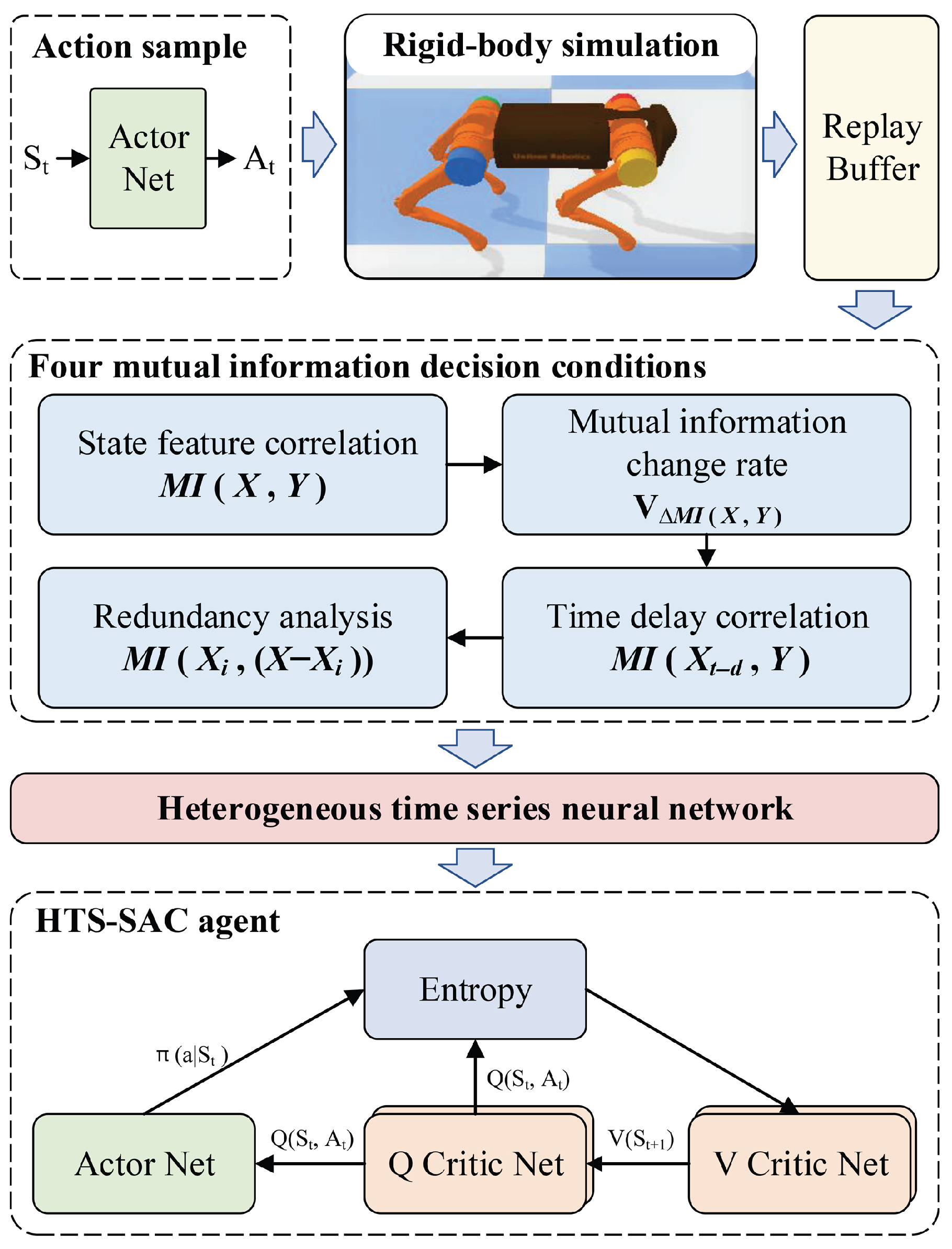
The current DRL-based methods overlook useful information of historical time-series data that can serve as a reliable source for optimizing strategies. Figure 1 shows the overall framework of the HTS-SAC algorithm. First, we adopt the traditionally trained SAC method to construct the initial experience replay buffer for the quadruped robot. Second, to address the issue of the low utilization of historical time-series data, we have designed four relevant decision-making criteria based on k-nearest neighbor mutual information to perform feature selection using data from the experience replay buffer. Finally, based on the new feature sequences after feature selection, we have designed an HTS-SAC model incorporating a heterogeneous time-series neural network to learn a better strategy.

2.1. Mutual Information Theory

The mutual information can fully show the degree of correlation between variables, and its concept comes from entropy in information theory.

Entropy is used to express the degree of uncertainty of random variables and the amount of information in random variables, which is often called information entropy. Set $\mathit{X}$ as a discrete random variable with a range of $D=\left\{x_i|i=1,\cdots ,N\right\}$; then, its entropy is defined as

$$H\left(\mathit{X}\right)=-\sum _i^{N}P\left(x_i\right)\log P\left(x_i\right),$$

(1)

where $P\left(x_i\right)$ denotes the probability that $\mathit{X}$ chooses $x_i$. When the base of the logarithmic function is 2, the unit of entropy is a bit.

Set $\mathit{X}$ and $\mathit{Y}$ as two discrete random variables; then, the mutual information between $\mathit{X}$ and $\mathit{Y}$ is defined as

$$MI(\mathit{X},\mathit{Y})=H\left(\mathit{X}\right)+H\left(\mathit{Y}\right)-H(\mathit{X},\mathit{Y}).$$

(2)

The k-nearest neighbor mutual information method applies the estimation method in the sample space and can directly calculate the high-dimensional mutual information. Assuming that there are N feature sample points $q_i=(x_i,y_i)$ in $Q=(\mathit{X},\mathit{Y})$, $i=1,\cdots ,N$, the k-nearest neighbor mutual information of random variables $\mathit{X}$ and $\mathit{Y}$ is defined as

$$MI(\mathit{X},\mathit{Y})=\psi \left(k\right)-〈\psi (n_x+1)+\psi (n_y+1)〉+\psi \left(N\right),$$

(3)

where $n_x$ denotes the number of sample points whose distance from point $x_i$ is less than ${\epsilon }_i/2$. Here, ${\epsilon }_i/2$ denotes the nearest distance between $q_i$ and the k-th point, and $n_y$ is denoted similarly. $\psi \left(k\right)$ is a Digamma function calculated by the following iteration:

$$\psi \left(1\right)=-0.5772516,$$

(4)

$$\psi (k+1)=\psi \left(k\right)+1/k.$$

(5)

2.2. Four Mutual Information Decision Conditions

Based on the k-nearest neighbor mutual information theory, we design four key feature decision conditions: the state feature correlation mutual information $MI(\mathit{X},\mathit{Y})$, the mutual information change rate $V_{\mathrm{\Delta }MI(\mathit{X},\mathit{Y})}$, the time delay correlation mutual information $MI({\mathit{X}}_{t-d},\mathit{Y})$ and the redundancy mutual information $MI({\mathit{X}}_i,(\mathit{X}-{\mathit{X}}_i))$.

a. The state feature correlation mutual information. Set the input variables as $\mathit{X}$; then, the mutual information between the output variable action reward $\mathit{Y}$ and the input variable set $\mathit{X}$ is defined as follows:

$$MI(\mathit{X},\mathit{Y})=\psi \left(k\right)-〈\psi (n_x+1)+\psi (n_y+1)〉+\psi \left(N\right).$$

(6)

By calculating the mutual information values of different state information variables, we can analyze the influence of different input state information variables on the locomotion state of the robot. Set the correlation threshold as ${\delta }_1>0$. When $MI(\mathit{X},\mathit{Y})>{\delta }_1$, it shows that the current variable is closely related, which is the key variable that affects the locomotion state of the robot.

b. The mutual information change rate. Select a variable ${\mathit{X}}_1$ as the reference variable, and combine the reference variable ${\mathit{X}}_1$ with other input state variables one by one to form a new set $\left\{{\mathit{X}}_{1+i}\right\}$, $i=2,\cdots ,m$. The mutual information of the reference variable ${\mathit{X}}_1$ and the new set $\left\{{\mathit{X}}_{1+i}\right\}$ is calculated, respectively. The change rate of mutual information is obtained by calculating the error of two mutual information. Define the rate of change of mutual information as follows:

$$V_{\mathrm{\Delta }MI(\mathit{X},\mathit{Y})}=\sqrt{MI{({\mathit{X}}_1,\mathit{Y})}^2-MI{({\mathit{X}}_{1+i},\mathit{Y})}^2}.$$

(7)

According to the information entropy, when ${\mathit{X}}_i$ is an independent variable, $V_{\mathrm{\Delta }MI(\mathit{X},\mathit{Y})}$ decreases; when ${\mathit{X}}_i$ is a key variable, $V_{\mathrm{\Delta }MI(\mathit{X},\mathit{Y})}$ increases. Set a correlation threshold ${\delta }_2$ to determine whether $V_{\mathrm{\Delta }MI(\mathit{X},\mathit{Y})}$ is a related variable. When $V_{\mathrm{\Delta }MI(\mathit{X},\mathit{Y})}>{\delta }_2$, it shows that the newly added variable ${\mathit{X}}_i$ is a related variable.

c. The time delay correlation mutual information. Set the action state reward $\mathit{Y}$ of the current state information ${\mathit{X}}_t$, and define ${\mathit{X}}_{t-d}$, $d=1,2,\cdots ,n$ as the state information at the historical moment with length d. The delay mutual information of state information is defined as follows:

$$\begin{array}{cc}\hfill & MI({\mathit{X}}_{t-d},\mathit{Y})\hfill \\ \hfill =& \psi \left(k\right)-〈\psi (n_{x_{t-d}}+1)+\psi (n_y+1)〉+\psi \left(N\right).\hfill \end{array}$$

(8)

Here, the delay correlation threshold is set as ${\delta }_3>0$. When $MI({\mathit{X}}_{t-d},\mathit{Y})>{\delta }_3$, it indicates that the state feature information of the current moment is a strong correlation feature.

d. The redundancy mutual information. After selecting the key feature variables through mutual information and mutual information change rate, it is necessary to analyze the redundancy of the feature information. The removal of redundant variables can effectively reduce data dimensions while improving the training speed. The redundant mutual information between ${\mathit{X}}_i$ and $\mathit{X}$ is defined as follows:

$$\begin{array}{cc}\hfill & MI({\mathit{X}}_i,(\mathit{X}-{\mathit{X}}_i))\hfill \\ \hfill =& \psi \left(k\right)-〈\psi (n_{x_i}+1)+\psi (n_{x-x_i}+1)〉+\psi \left(N\right).\hfill \end{array}$$

(9)

Here, the threshold of redundancy correlation is set as ${\delta }_4>0$. When $MI({\mathit{X}}_i,(\mathit{X}-{\mathit{X}}_i))<{\delta }_4$, it means that the variable is redundant and needs to be eliminated.

The final optimized feature results need to meet all four decision conditions simultaneously. In this way, the proposed method can enhance the effective utilization of the historical information while optimizing features to avoid dimension explosion.

3. Gait Learning Method by HTS-SAC

3.1. Heterogeneous Time-Series Method

In this subsection, we design a heterogeneous time-series neural network based on feature selection. We integrate heterogeneous time-series neural networks with the SAC to construct the HTS-SAC model, which can use heterogeneous time-series datasets and learn high-level features. The structure of the heterogeneous time-series neural network is shown in Figure 2.

The detailed design of the network is as follows. According to the correlation and redundancy mutual information, different time delays d are designed for a single input variable ${\mathit{X}}_i$ to form a heterogeneous time-series input layer $\mathit{S}$. When ${\mathit{X}}_i$ is strongly correlated, it will appropriately increase the length of the historical time series to use more feature information of the historical moment. When ${\mathit{X}}_i$ is weakly correlated, it will reduce the length of data appropriately to shorten the training time of the model. The heterogeneous time-series neural network is designed based on the importance of historical information from different dimensions.

3.2. HTS-SAC Algorithm

The soft actor–critic (SAC) is an off-policy DRL algorithm [28]. The entropy regularization is introduced into policy training to enlarge the policy searching space. However, the conventional SAC method only considers the current state ${\mathit{S}}_t$ and the previous state ${\mathit{S}}_{t-1}$, while ignoring the impact of longer historical time-series data ${\mathit{S}}_{t-m}(m=1,2,...,n)$. To resolve this issue, we design an HTS-SAC control framework for unmanned quadruped robots that integrates heterogeneous time-series neural networks. As a result, the actor network of HTS-SAC has the capability to learn the features of state variables from heterogeneous historical time series.

The observation space ${\mathit{S}}_t$ should contain all observable information related to the task. All the observation elements at $t=t_i$ are defined as

$${\mathit{S}}_{t_i}=〈{\mathit{p}}_{t_i},{\mathit{\varphi }}_{t_i},{\mathit{\omega }}_{t_i},{\mathit{\psi }}_{t_i},{\mathit{\delta }}_{t_i},{\mathbf{\Theta }}_{t_i}〉,$$

(10)

where ${\mathit{p}}_{t_i}$ is the robot base position, ${\mathit{\varphi }}_{t_i}$ and ${\mathit{\omega }}_{t_i}$ are the base angles and angular velocities, ${\mathit{\psi }}_{t_i}$ and ${\mathit{\delta }}_{t_i}$ are the joint angles and positions, and ${\mathbf{\Theta }}_{t_i}$ is the foot contact detection.

A non-deterministic control policy $\mathit{\pi }$ gives the conditional probability density $\mathit{\pi }({\mathit{a}}_t\mid {\mathit{s}}_t)$ of taking action ${\mathit{a}}_t$ in the state ${\mathit{s}}_t$. The formula for calculating entropy H is

$$H\left(\mathit{\pi }(·\mid {\mathit{s}}_t)\right)=E_{\mathit{\pi }}\left[-\ln \mathit{\pi }(·\mid {\mathit{s}}_t)\right].$$

(11)

The policy entropy is a measure to estimate the randomness of the actions that an agent can take in a given state. Higher entropy indicates policies with higher uncertainty and stronger exploration ability. By introducing the entropy $H\left(\mathit{\pi }(·\mid {\mathit{s}}_t)\right)$ into a part of the reward $\mathit{r}$, the agent will receive an additional entropy-related reward at each step of the exploration. The reward function $J\left(\mathit{\pi }\right)$ at the maximum policy entropy is defined as

$$J\left(\mathit{\pi }\right)=E_{\pi }\left[\sum _{t=0}^{T}r({\mathit{s}}_t,{\mathit{a}}_t)+\alpha H\left(\mathit{\pi }(·\mid {\mathit{s}}_t)\right)\right],$$

(12)

where $\mathit{r}$ is the reward of the agent taking action ${\mathit{a}}_t$ in the state ${\mathit{s}}_t$. $\alpha$ is the regularization coefficient of entropy, which is used to control the randomness degree of the optimal policy and the importance of the upper policy entropy to the reward. The state–action value function $Q(·)$ is defined as

$$\begin{array}{cc}\hfill Q_t^{\mathit{\pi }}({\mathit{s}}_t,{\mathit{a}}_t)& =r({\mathit{s}}_t,{\mathit{a}}_t)\hfill \\ \hfill & +E_{\mathit{\pi }}\left[\sum _{l=1}^{T}r({\mathit{s}}_{t+1}+{\mathit{a}}_{t+1})-\alpha \log \mathit{\pi }({\mathit{a}}_{t+l}\mid {\mathit{s}}_{t+l})\right].\hfill \end{array}$$

(13)

According to $Q_t^{\mathit{\pi }}({\mathit{s}}_t,{\mathit{a}}_t)$, the state value function $V(·)$ is defined as

$$V_t^{\mathit{\pi }}\left({\mathit{s}}_t\right)=E\left[Q_t^{\mathit{\pi }}({\mathit{s}}_t,{\mathit{a}}_t)-\alpha \log \mathit{\pi }({\mathit{a}}_t\mid {\mathit{s}}_t)\right].$$

(14)

According to (13) and (14), $Q_t^{\mathit{\pi }}({\mathit{s}}_t,{\mathit{a}}_t)$ can be expressed as $V_t^{\mathit{\pi }}\left({\mathit{s}}_t\right)$.

$$Q_t^{\mathit{\pi }}({\mathit{s}}_t,{\mathit{a}}_t)=r({\mathit{s}}_t,{\mathit{a}}_t)+E_{{\mathit{s}}_{t+1}\sim p({\mathit{s}}_{t+1}\mid {\mathit{s}}_t,{\mathit{a}}_t)}\left[V_{t+1}^{\mathit{\pi }}\left({\mathit{s}}_{t+1}\right)\right],$$

(15)

where (15) is also known as the soft Bellman equation.

For continuous state–action tasks, it is necessary to introduce function approximation. Define the parameter of the soft state value function $V(·)$ as $\varphi$. The parameter of the state–action value function $Q(·)$ is $\psi$, and the parameter of the policy function $\mathit{\pi }(·\mid \mathit{s})$ is $\theta$. According to the definition of state value function, the loss function $L_V\left(\varphi \right)$ of $V_t^{\mathit{\pi }}\left({\mathit{s}}_t\right)$ is obtained.

$$\begin{array}{cc}\hfill & L_V\left(\varphi \right)\hfill \\ \hfill =& E_{\mathit{s}\sim p\left(\mathit{s}\right)}\left[V_{\varphi }\left(\mathit{s}\right)-E_{\mathit{a}\sim \mathit{\pi }(\mathit{a}\mid \mathit{s})}\left[Q(\mathit{s},\mathit{a})-\alpha \log \mathit{\pi }(\mathit{a}\mid \mathit{s})\mid {\mathit{s}}^2\right]\right],\hfill \end{array}$$

(16)

Action $\mathit{a}$ represents the actor network under the condition of policy $\mathit{\pi }(·\mid \mathit{s})$. Here, $\mathit{a}$ is calculated by a neural network containing noise:

$$\mathit{a}=f_{\theta }(\mathit{ϵ};\mathit{s}),$$

(17)

where $\mathit{ϵ}$ is the input noise vector, sampled from a fixed distribution (such as a spherical Gaussian distribution).

According to the soft Bellman equation, the loss function $L_Q\left(\psi \right)$ of Q-value function $Q_t^{\mathit{\pi }}({\mathit{s}}_t,{\mathit{a}}_t)$ is defined as follows:

$$L_Q\left(\psi \right)=E_{\mathit{\pi }}\left[Q_{\psi }(\mathit{s},\mathit{a})-{(r(\mathit{s},\mathit{a})+\gamma V_{\varphi }\left({\mathit{s}}^{\prime }\right))}^2\right].$$

(18)

Equation (12) is rewritten as a reward function in the form of KL-divergence:

$$J\left(\mathit{\pi }\right)=-E_{{\mathit{s}}_0\sim p\left({\mathit{s}}_0\right)}\left[D_{KL}(\mathit{\pi }(·\mid {\mathit{s}}_0)\cdots \exp \left({\displaystyle \frac{1}{\alpha }}{Q}_0^{\mathit{\pi }}({\mathit{s}}_0,·)\right))\right]+b,$$

(19)

where b is a constant. The loss function $L_{\mathit{\pi }}\left(\theta \right)$ of the updated policy is obtained by maximizing the reward $J\left(\mathit{\pi }\right)$:

$$L_{\mathit{\pi }}\left(\theta \right)=E_{\mathit{s}\sim p\left(\mathit{s}\right)}\left[E_{\mathit{a}\sim \mathit{\pi }(\mathit{a}\mid \mathit{s})}\left[\alpha \log {\mathit{\pi }}_{\theta }(\mathit{a}\mid \mathit{s})-Q_{\psi }(\mathit{s},\mathit{a})\mid \mathit{s}\right]\right].$$

(20)

Finally, the gradient descent method is used to minimize the above three loss functions $L_V\left(\varphi \right)$, $L_Q\left(\psi \right)$, and $L_{\mathit{\pi }}\left(\theta \right)$, and the optimal policy $\mathit{\pi }$ is obtained. The detailed steps of the HTS-SAC method are shown in Algorithm 1.

Algorithm 1 HTS-SAC algorithm

Require: Initialize the actor network parameter $\theta$ and critic network parameters $\varphi ,\psi$, target network parameter ${\varphi }_{targ}$, experience pool $\mathcal{D}$. for each iteration do    for each environment step do      ${\mathit{a}}_t\leftarrow {\mathit{\pi }}_{\theta }({\mathit{a}}_t\mid {\mathit{s}}_t)$      ${\mathit{s}}_{t+1}\leftarrow p({\mathit{s}}_{t+1}\mid {\mathit{s}}_t,{\mathit{a}}_t)$      $\mathcal{D}\leftarrow \mathcal{D}\cup \left\{{\mathit{s}}_t,{\mathit{a}}_t,r({\mathit{s}}_t,{\mathit{a}}_t),{\mathit{s}}_{t+1}\right\}$    end for    while experience pool $\mathcal{D}$ is full do      for each variable do         ${\mathit{X}}^{\prime }\leftarrow \left\{\begin{array}{c}MI(\mathit{X},\mathit{Y})>{\delta }_1\hfill \\ V_{\mathrm{\Delta }MI(\mathit{X},\mathit{Y})}>{\delta }_2\hfill \\ MI({\mathit{X}}_{t-d},\mathit{Y})>{\delta }_3\hfill \\ MI({\mathit{X}}_i,(\mathit{X}-{\mathit{X}}_i))<{\delta }_4\hfill \end{array}\right.$      end for      Use ${\mathit{X}}^{\prime }$ to update the experience pool ${\mathcal{D}}^{\prime }\leftarrow \mathcal{D}$      Construct HTS neural network based on ${\mathcal{D}}^{\prime }$    end while    for each gradient step do      $\varphi \leftarrow \varphi -{\lambda }_V{\widehat{\nabla }}_{\varphi }{J}_V\left(\varphi \right)$      ${\psi }_i\leftarrow {\psi }_i-{\lambda }_Q{\widehat{\nabla }}_{{\psi }_i}{J}_Q\left({\psi }_i\right)$$for$$i\in \left\{1,2\right\}$      $\theta \leftarrow \theta -{\lambda }_{\mathit{\pi }}{\widehat{\nabla }}_{\theta }{J}_{\mathit{\pi }}\left(\theta \right)$      ${\varphi }_{targ}\leftarrow \rho \varphi +(1-\rho ){\varphi }_{targ}$    end for end for

4. Numerical Simulation

In this section, we compare the twin delayed deep deterministic policy gradient (TD3), the deep deterministic policy gradient (DDPG), the proximal policy optimization (PPO), the traditional SAC, and the time-delay soft actor–critic (TD-SAC) with the HTS-SAC proposed in this paper. The TD-SAC method is a comparative method we constructed, and this method only utilizes a large amount of historical state data without feature optimization. We use the PyBullet robot simulation system for testing. PyBullet has excellent rendering and collision detection details, which can simulate the real world with high fidelity. In addition, it is packaged into a Python (v3.8.2) module for robot simulation and experimentation and provides forward/reverse kinematics, forward/reverse dynamics, collision detection, ray intersection queries and other functions. The parameters of PyBullet are shown in

Table 1. Parameters of PyBullet.

Parameters	Parameters Value
Fixed time step	0.00416 s
Solver iterations	50
solver type	Projected Gauss–Seidel
sensor noise model	Gaussian noise
Robot mass	4.7 kg
Friction	0.5
Restitution	(0.02, 0.03, 0.04)

. The Laikago-a1 quadruped robot is employed for simulation test. We set the actuator delay as 2 ms. The joint actuator uses position control, with its PID gains as follows: kp = 60, kd = 1. In addition, in order to simulate the real robot environment, we also add noise to the collected data from sensors.

The flowchart of the HTS-SAC program is shown in Figure 3. First, we use the traditional SAC method to collect 10,000 data entries in the initial experience replay buffer (denoted as D), with the training scenario set on flat ground. 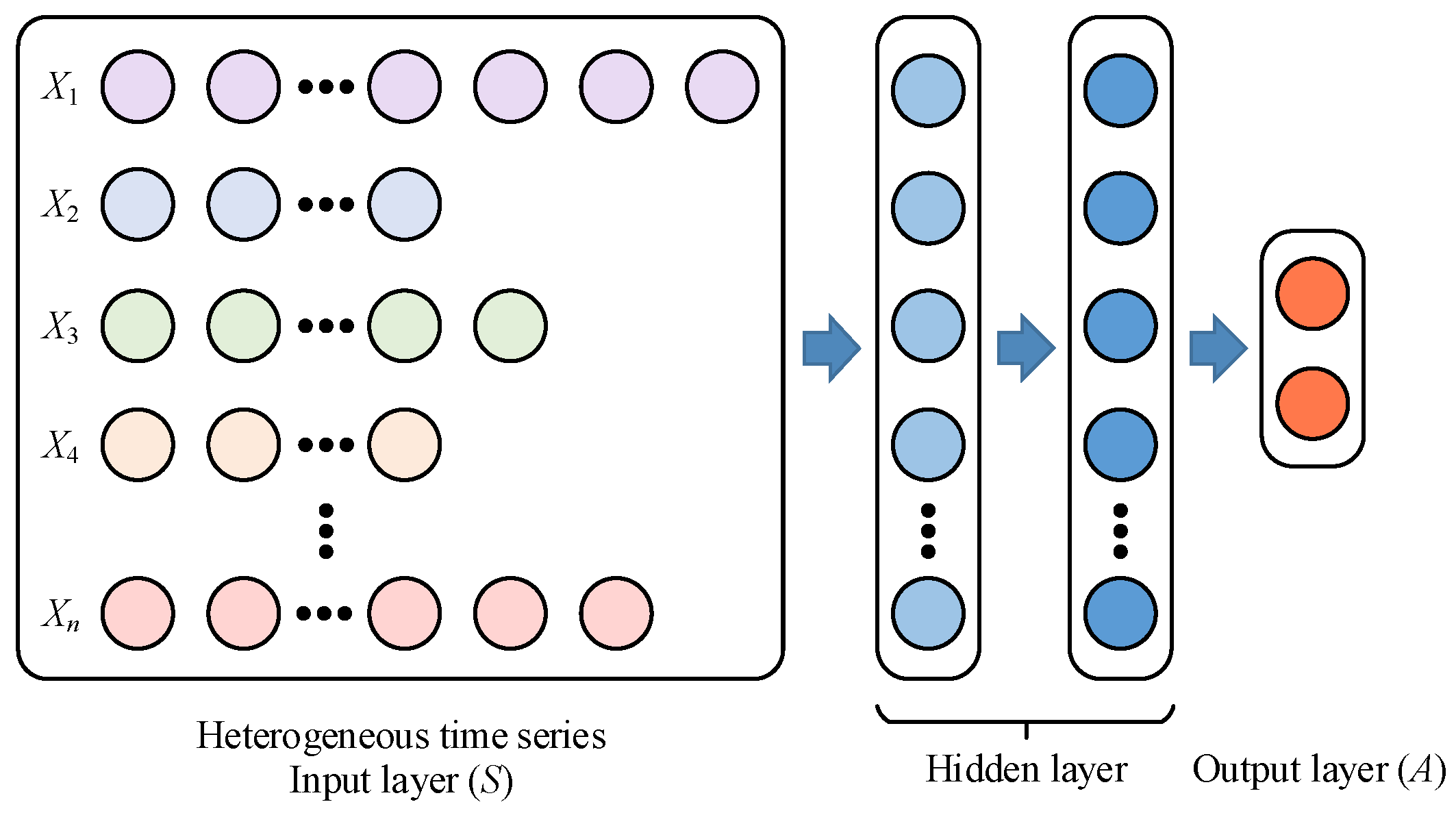Second, the data D from the experience replay buffer is fed into our four mutual information decision criteria, and through feature optimization and selection, new time-series features and a new experience replay buffer $D^{\prime }$ are generated. Then, based on the new time-series features after feature optimization, a heterogeneous time-series neural network is designed. Finally, the heterogeneous time-series neural network is incorporated into the HTS-SAC model to form a new HTS-SAC model, and the final model is obtained through iterative training for testing.

The main difference between the HTS-SAC and the SAC is the mutual information feature selection and the heterogeneous time-series neural network, as shown in the red dashed box in Figure 3.

We choose the input of the SAC policy network as the initial state set $\left\{\mathit{X}\right\}$, which is the observation information obtained by four sensors of the Laikago-a1 quadruped robot. The content of the set $\left\{\mathit{X}\right\}$ is as follows: the data of the base-displacement sensor in three orientations $({\mathit{p}}_x,{\mathit{p}}_y,{\mathit{p}}_z)$, the angle and angular velocity data of the IMU sensor $({\mathit{r}}_x,{\mathit{r}}_y,{\mathit{r}}_z,{\mathit{r}}_x^{rate},{\mathit{r}}_y^{rate},{\mathit{r}}_z^{rate})$, joint angles of 12 joints $({\mathit{j}}_1^a,{\mathit{j}}_2^a,\cdots ,{\mathit{j}}_{12}^a)$, joint positions of 12 joints $({\mathit{j}}_1^p,{\mathit{j}}_2^p,\cdots ,{\mathit{j}}_{12}^p)$, and dataset $({\mathit{c}}_{FL},{\mathit{c}}_{FR},{\mathit{c}}_{BL},{\mathit{c}}_{BR})$ from the foot-contact sensor for determining whether the foot touches the ground or not.

The action space is the output of the actor network, which corresponds to the position information of the 12 joints of the unmanned quadruped robot. The reward function is designed as follows:

$${\mathit{r}}_t={\mathit{X}}_1\left(t\right)-{\mathit{X}}_1(t-1),$$

(21)

where the reward ${\mathit{r}}_t$ is expressed as the difference between the X-axis displacement of the current time and the previous time. Note that the reward in (19) is a universal design which can reduce the impact of the reward function on the comparative studies.

4.1. Feature Selection of Heterogeneous Time Series

In the feature selection simulation, 10,000 sets of data from the initial experience pool are used as the training data. 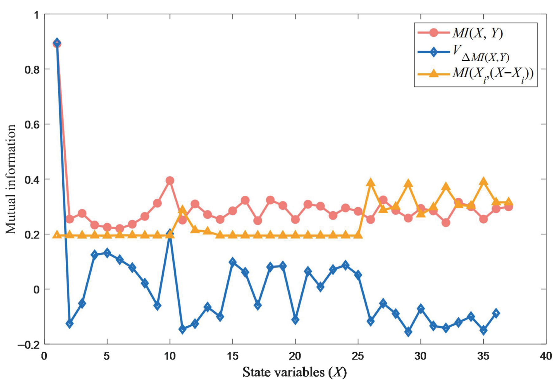The test results of the state feature correlation mutual information $MI(\mathit{X},\mathit{Y})$, the mutual information change rate $V_{\mathrm{\Delta }MI(\mathit{X},\mathit{Y})}$, and the redundancy mutual information $MI({\mathit{X}}_i,(\mathit{X}-{\mathit{X}}_i))$ are shown in Figure 4. The red line represents the state feature correlation mutual information $MI(\mathit{X},\mathit{Y})$. It can be observed that when $MI(\mathit{X},\mathit{Y})>0.3$, the corresponding variable is strongly correlated, which is the key variable we need. That is, ${\mathit{X}}_1$ (position of the X-axis) and ${\mathit{X}}_{10}$ (angular velocity of the Z-axis) have strong correlations. The blue line indicates the mutual information change rate $V_{\mathrm{\Delta }MI(\mathit{X},\mathit{Y})}$. We choose ${\mathit{X}}_{37}$ as the benchmark variable and combine it with ${\mathit{X}}_i$, $i=1,2,\dots ,36$ to form a new set $\left\{{\mathit{X}}_{37+i}\right\}$. The change rate of mutual information is determined by calculating the difference between $\left\{{\mathit{X}}_{37+i}\right\}$ and ${\mathit{X}}_{37}$. When $V_{\mathrm{\Delta }MI(\mathit{X},\mathit{Y})}>0$, it shows that the newly added variable ${\mathit{X}}_i$ is the correlated variable. The yellow line is the redundancy mutual information $MI({\mathit{X}}_i,(\mathit{X}-{\mathit{X}}_i))$. When $MI({\mathit{X}}_i,(\mathit{X}-{\mathit{X}}_i))>0.27$, it indicates that the variable ${\mathit{X}}_i$ is redundant and should be eliminated. According to the mutual information results in Figure 4, we set ${\delta }_1=0.3$, ${\delta }_2=0$, and ${\delta }_4=0.27$. As a result, the key feature variables are determined to be $({\mathit{X}}_1,{\mathit{X}}_{10},{\mathit{X}}_{16},{\mathit{X}}_{18},{\mathit{X}}_{19},{\mathit{X}}_{21},{\mathit{X}}_{22})$.

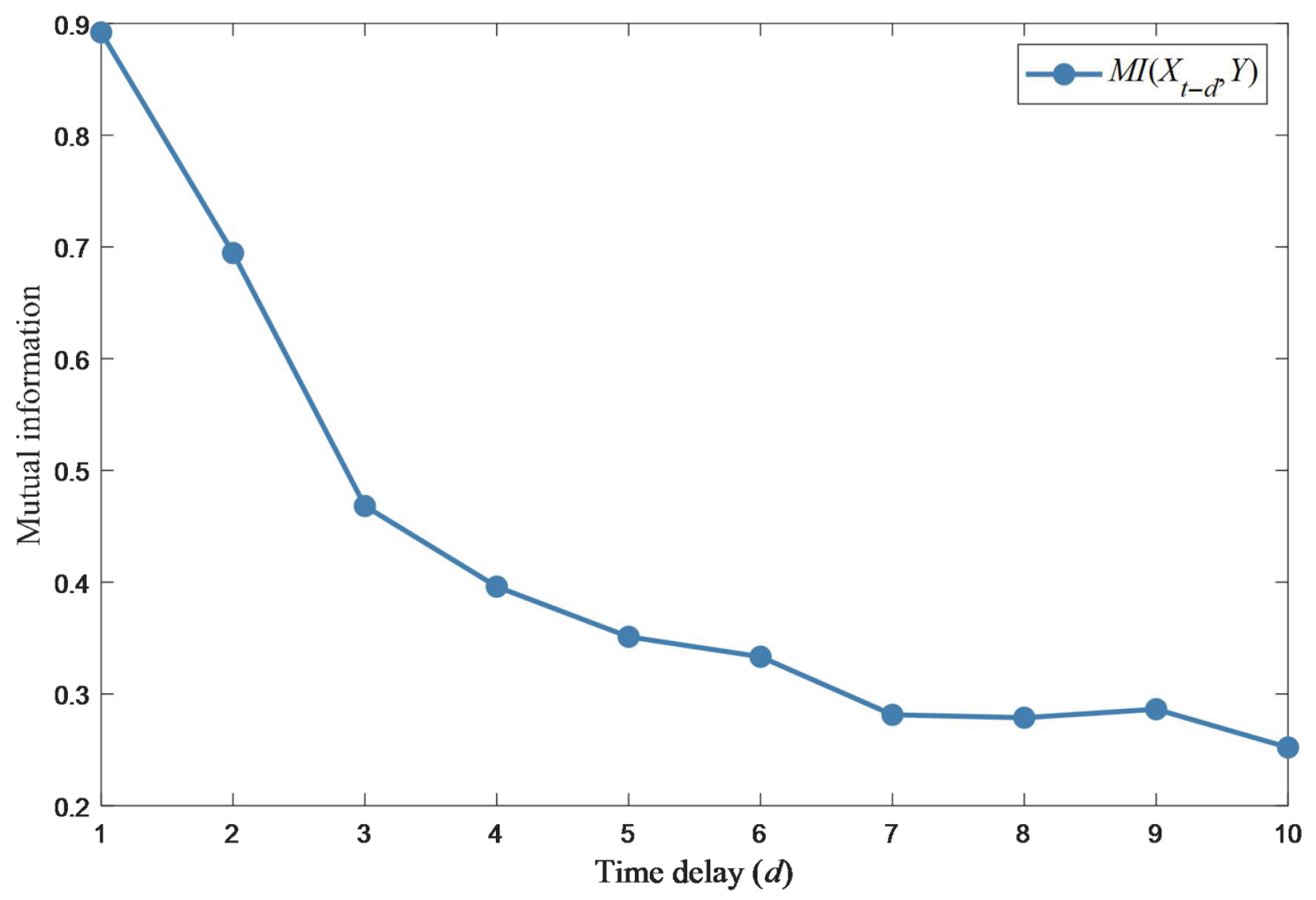
The time delay correlation mutual information $MI({\mathit{X}}_{t-d},\mathit{Y})$ for delay lengths $d\in [1,10]$ can be seen in Figure 5. When $d=1$ and $d=2$, the corresponding variables have strong correlations. As d increases, the correlation of variables gradually reduces. According to the curve of $MI({\mathit{X}}_{t-d},\mathit{Y})$, we set the delay correlation threshold ${\delta }_3$ as 0.3. When $MI({\mathit{X}}_{t-d},\mathit{Y})>{\delta }_3$, it shows that the variable has strong correlation and should be retained.

According to the mutual information decision conditions, the key features that affect policy learning can be obtained. Therefore, we choose ${\mathit{X}}_1$ and ${\mathit{X}}_{10}$ with a long historical time series, with $d=6$. ${\mathit{X}}_{16},{\mathit{X}}_{18},{\mathit{X}}_{19},{\mathit{X}}_{21},{\mathit{X}}_{22}$ are set to medium-length historical time series, with $d=3$. Other variables are set to a short historical time series, with $d=2$. In this way, a heterogeneous time-series input layer with a non-uniform length is designed. Then, we set the HTS-SAC input layer dimension as 87 (corresponding to the data with heterogeneous time series). The SAC input layer dimension is 37 (corresponding to the data with a time-series length of 1). The TD-SAC input layer dimension is 370 (corresponding to the data with a time-series length of 10).

4.2. Algorithm Simulation

We test the DDPG, PPO, TD3, SAC, TD-SAC, and HTS-SAC methods on different terrains using the Laikago-a1 quadruped robot simulation model. The advantages and disadvantages of the methods are analyzed by comparing the forward running.

The parameters of the agile locomotion control model of the unmanned quadruped robot based on HTS-SAC algorithm are shown in

Table 2. Parameters of locomotion control model of the unmanned quadruped robot.

Parameters	Parameters Value
Actor fc layer params	(512, 512)
Critic fc layer params	(512, 512)
Gamma	0.99
Epochs	1000
Steps per epoch	4000
Replay size	1,000,000
Batch size	100
Actor learning rate	0.001
Critic learning rate	0.001

. The parameters are continuously optimized during training and testing. Here are some adjustment guidance and rules. Layer params: Increases sequentially from 128 and does not exceed 1024. Gamma: Gamma represents the discount factor. A larger Gamma indicates longer rewards, usually increasing from 0.99 to 0.999. Epochs: Usually increase from 100 but generally do not exceed ${10}^4$. Steps per epoch: Start from 1000 and generally do not exceed 5000. Their product represents the total number of steps, which is generally greater than ${10}^5$. When the training exceeds ${10}^6$ steps and still does not converge, it indicates that the parameters are not suitable and the model need to be retrained. Replay size: Usually increases from ${10}^5$ and ranges from ${10}^5$ to ${10}^6$. Batch size: We usually choose a batch size that is equivalent to or smaller than the layer params. Learning rate: Generally, it decreases sequentially starting from $1\times {10}^{-2}$, ranging from $1\times {10}^{-2}$ to $1\times {10}^{-5}$.

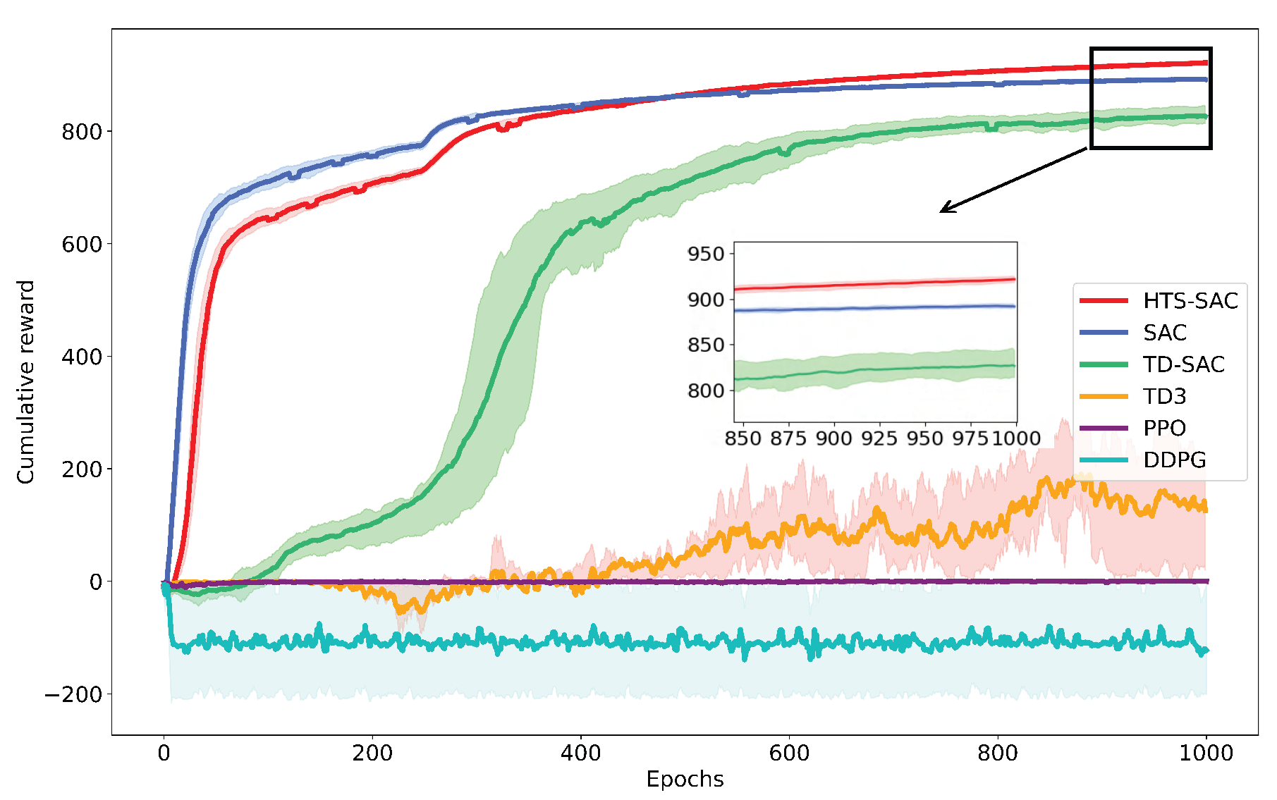
Figure 6 plots the cumulative training reward simulation results across 20 runs for each method on the selected map, together with 80% confidence intervals. All algorithms are trained and tested using the Laikago robot under fair conditions. The training results for TD-SAC and SAC are 828.61 and 885.32, respectively. However, the DDPG and PPO methods cannot converge, despite extensive network optimization and hyperparameter adjustment work, and the training performance of TD3 is poor. Although the early rewards of HTS-SAC are lower than those of SAC, it is significantly better than other methods after 350 epochs. The final cumulative reward is 923.99, which shows that the proposed HTS-SAC method can converge stably and learn the optimal locomotion policy by using heterogeneous time-series data. The numerical results of the cumulative training rewards for each method can be found in

Table 3. Cumulative training rewards for different methods.

Methods	Rewards
DDPG	−122
PPO	−0.17
TD3	125
SAC	891
TD-SAC	826
HTS-SAC	923

.

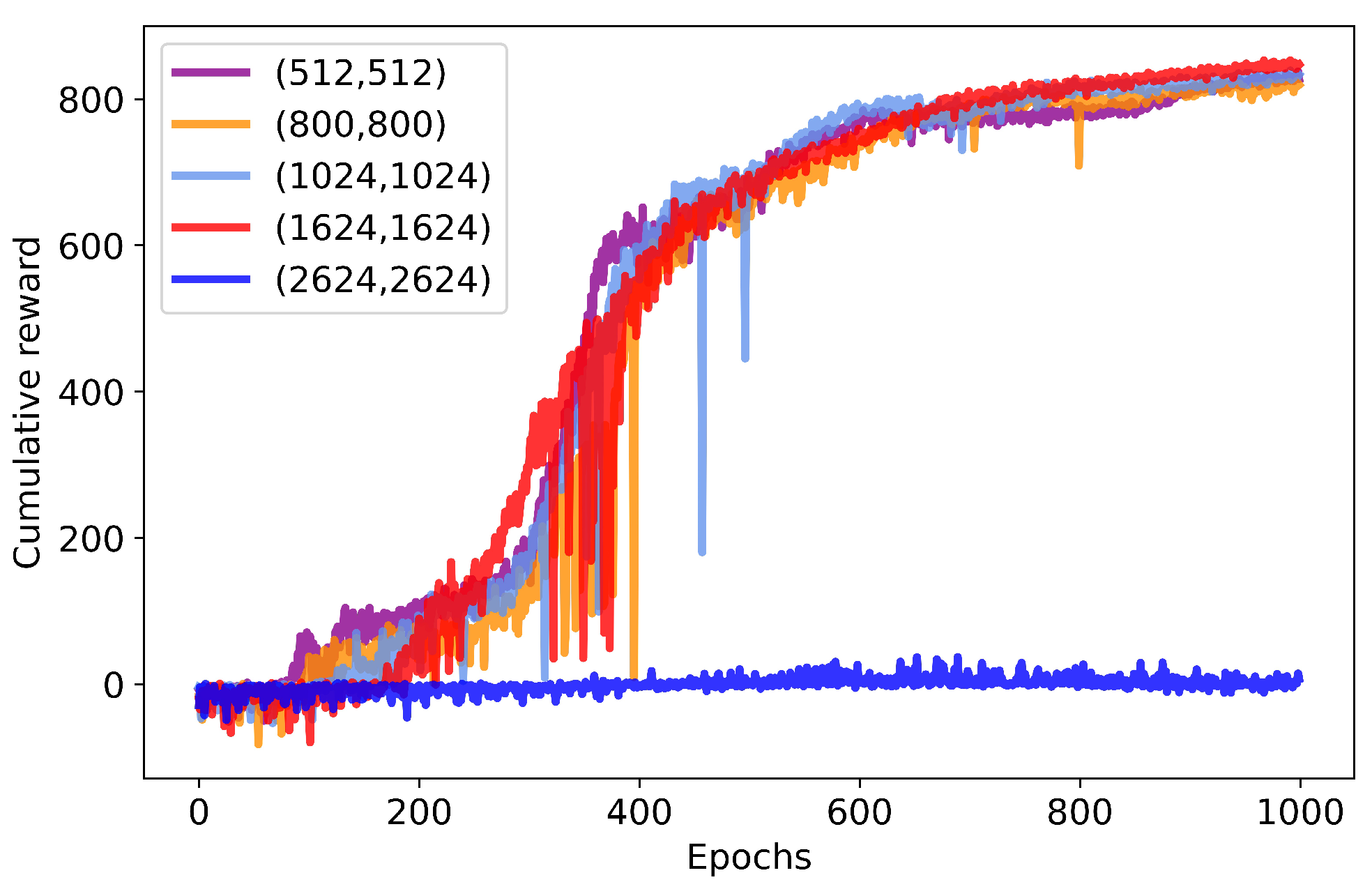
We test different TD-SAC network structures to provide fair comparison conditions, with the results shown in

Table 4. TD-SAC training results under different structural conditions.

Network Structure	Reward
(500, 500)	827
(800, 800)	828
(1024, 1024)	833
(1624, 1624)	847
(2624, 2624)	7.5

and Figure 7. The results indicate that increasing the complexity of the network structure leads to an increase in cumulative rewards, with the maximum not exceeding 847. Additionally, when the network structure exceeds (2624, 2624), the model fails to converge, resulting in a reward of only 7.5.

To verify the control performance and agility of the proposed method, we test four different DRL algorithms in four scenarios, flat ground, uphill and downhill slopes, stair waves, and real land, as shown in Figure 8. Figure 9 shows the speed curves of four methods on flat ground; each method underwent a forward running test of 1000 steps. The link to the robot’s test demonstration video is https://youtu.be/yD8dkU6z52I (accessed on 3 August 2025). 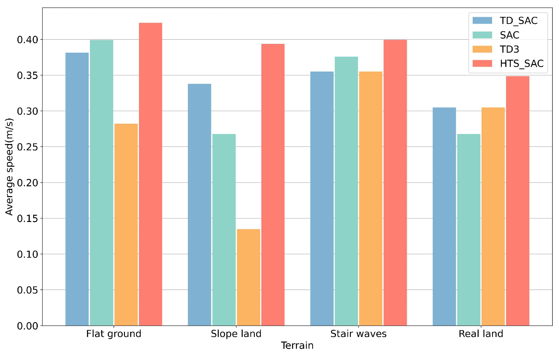The speed tests on the four different terrains are shown in Figure 10. We find that the proposed method has better locomotion speed and agility on all terrains, and the smallest velocity attenuation on complex terrains. The average speeds of the HTS-SAC, SAC, TD-SAC and TD3 on all terrains are 0.39 m/s, 0.33 m/s, 0.34 m/s, and 0.24 m/s, respectively.

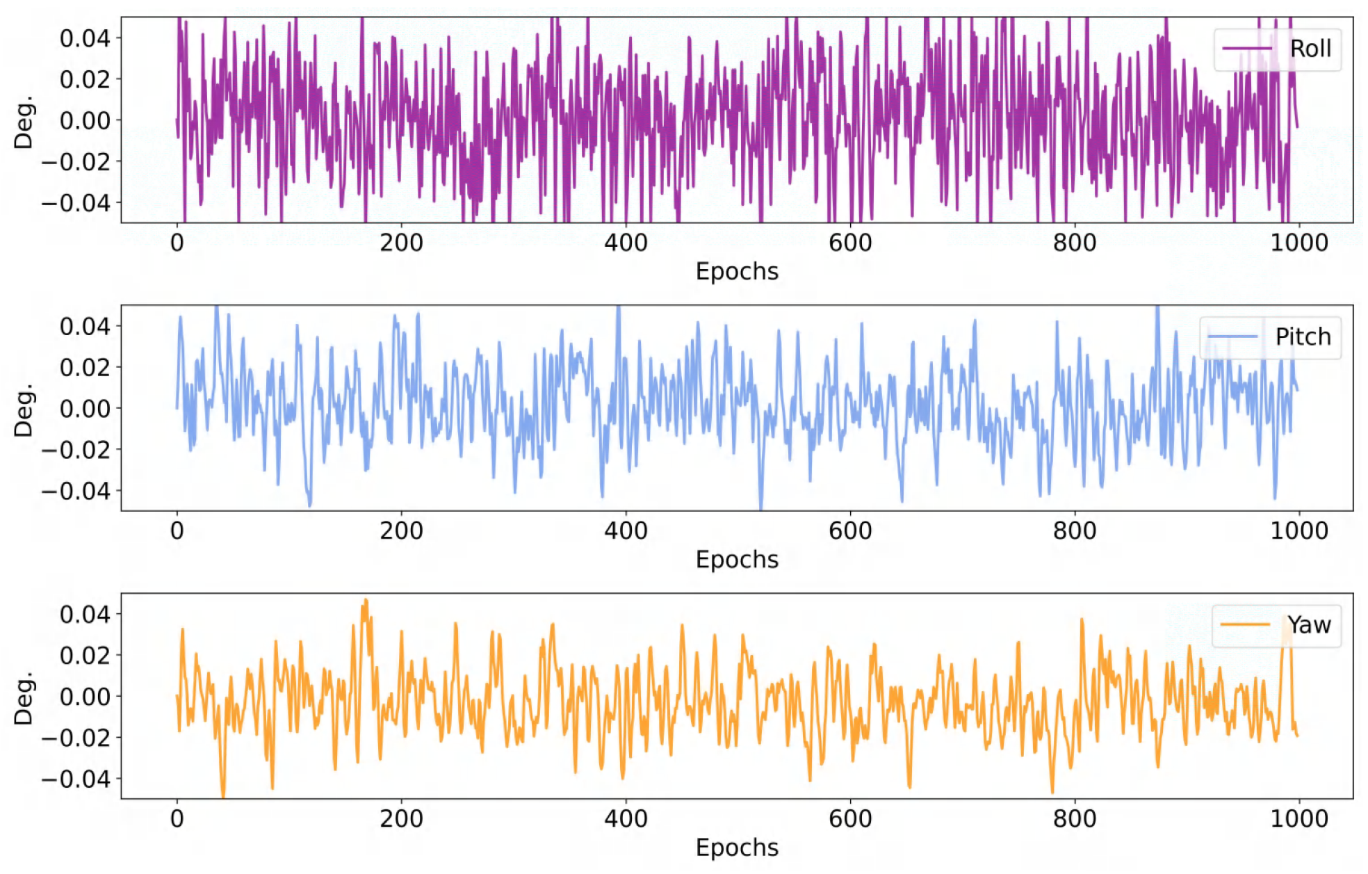
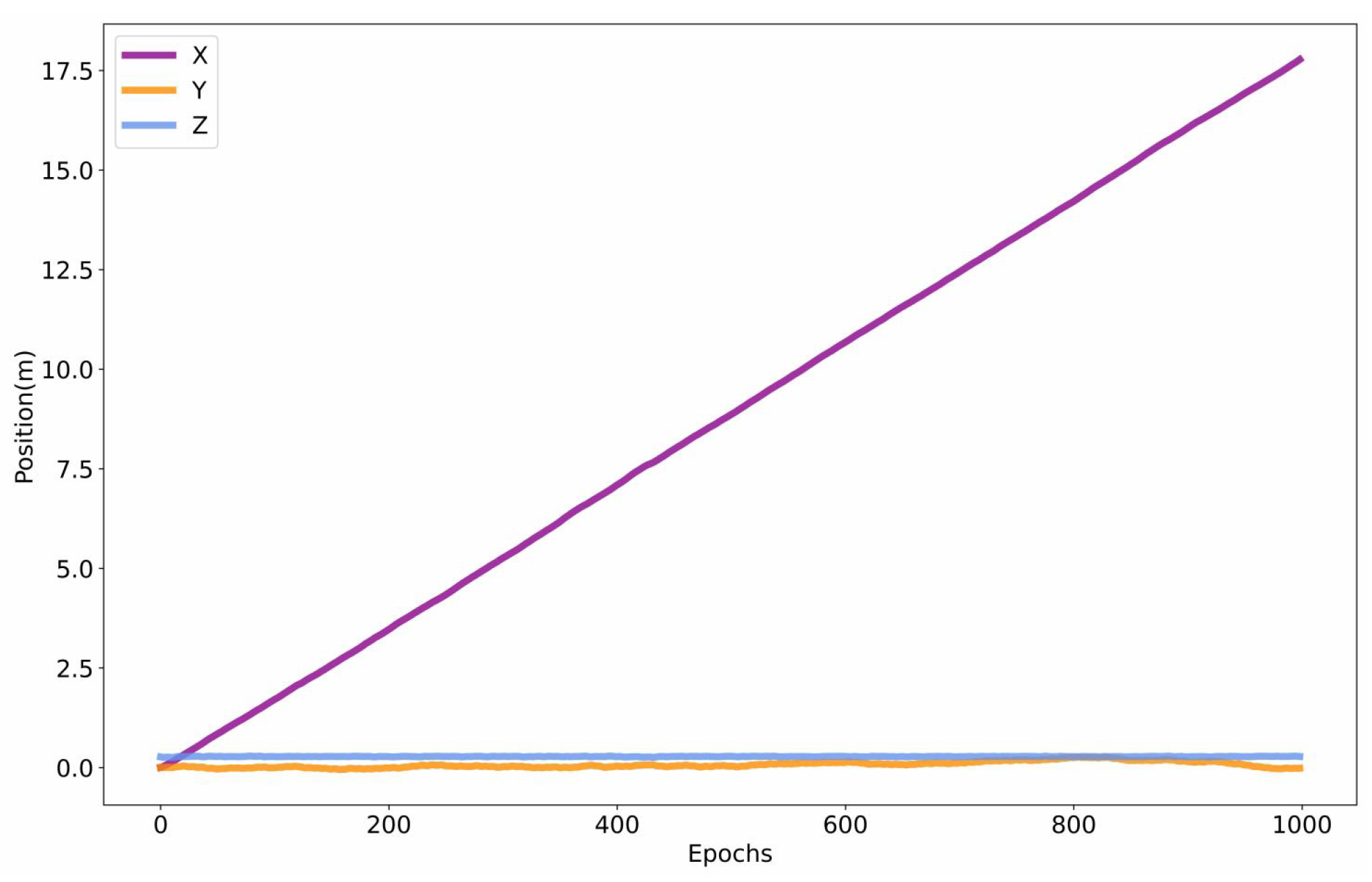
In addition, Figure 11 and Figure 12 show the real-time collection of robot position and angle information on flat ground using the proposed method. In particular, the results in Figure 11 show that the deviation of the robot’s locomotion trajectory on the Y-axis is small. The error on the Y-axis is 0.08, and the variance on the Y-axis is $6\times {10}^{-3}$. Figure 12 reflects the real-time angle changes in the tests, with all angle changes being less than 0.05 degrees.

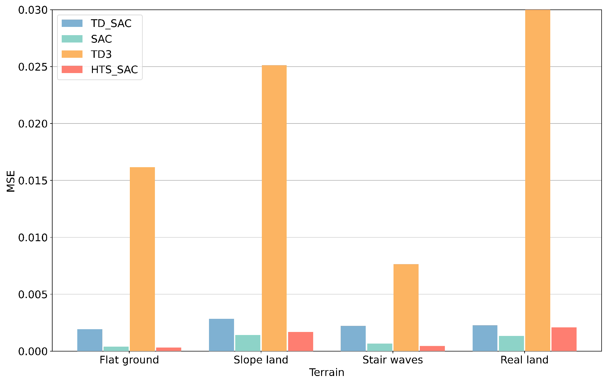
Figure 13 shows the angle mean squared error (MSE) of four methods on different terrains, which reflects the stability of the robot. The MSE results of the yaw angles of each method on different terrains are shown in

Table 5. The yaw angle MSE of four methods on different terrains.

Methods	Flat Ground	Slope Land	Stair Waves	Real Land
TD3	$1.15\times {10}^{-2}$	$1.04\times {10}^{-2}$	$1.52\times {10}^{-2}$	$8.99\times {10}^{-3}$
SAC	$2.23\times {10}^{-4}$	$5.39\times {10}^{-4}$	$4.94\times {10}^{-4}$	$1.42\times {10}^{-3}$
TD-SAC	$1.21\times {10}^{-3}$	$4.08\times {10}^{-3}$	$1.39\times {10}^{-3}$	$2.61\times {10}^{-3}$
HTS-SAC	$1.73\times {10}^{-4}$	$2.39\times {10}^{-4}$	$2.38\times {10}^{-4}$	$4.21\times {10}^{-4}$

. The proposed method has the smallest errors on flat ground and stair wave terrain, while SAC has smaller errors on slope land and real land. Compared with the speed test results in Figure 10, although SAC has smaller errors, its speed attenuation is severe on uphill and downhill slopes and real land. In conclusion, the proposed method has the fastest locomotion speed on all terrains while maintaining smaller angle errors, which indicates that the proposed method has enhanced control performance and stability.

The comparative test results of different thresholds are shown in

Table 6. The training results of HTS-SAC with different threshold conditions.

Methods	${\mathit{\delta }}_1$	${\mathit{\delta }}_2$	${\mathit{\delta }}_3$	${\mathit{\delta }}_4$	Characteristic Number	Reward
HTS-SAC	0.3	0	0.3	0.27	87	924
Compare1	0.29	−0.05	0.3	0.28	125	906
Compare2	0.28	−0.1	0.3	0.29	165	896

. The results indicate that when we decrease ${\delta }_1$ and ${\delta }_2$ and increase ${\delta }_4$, obvious changes occur in feature dimensions and training cumulative rewards. The selection of thresholds currently relies on manual experience and needs to be continuously adjusted according to specific application scenarios.

Figure 14 shows the results of whether each of the four legs is in contact with the ground at each moment. In the figure, black circles indicate that the corresponding leg is in contact with the ground at the current moment, and red circles indicate that it is in the air at the current moment. During the test, the ground contact information was recorded starting from the moment the robot was set up; therefore, all four legs of the robot are in the air at step 0, and the robot starts to move from step = 3. We did not add any periodic constraints or rewards when training the proposed model, which makes the trained robot dog exhibit aperiodic foot movements during motion.

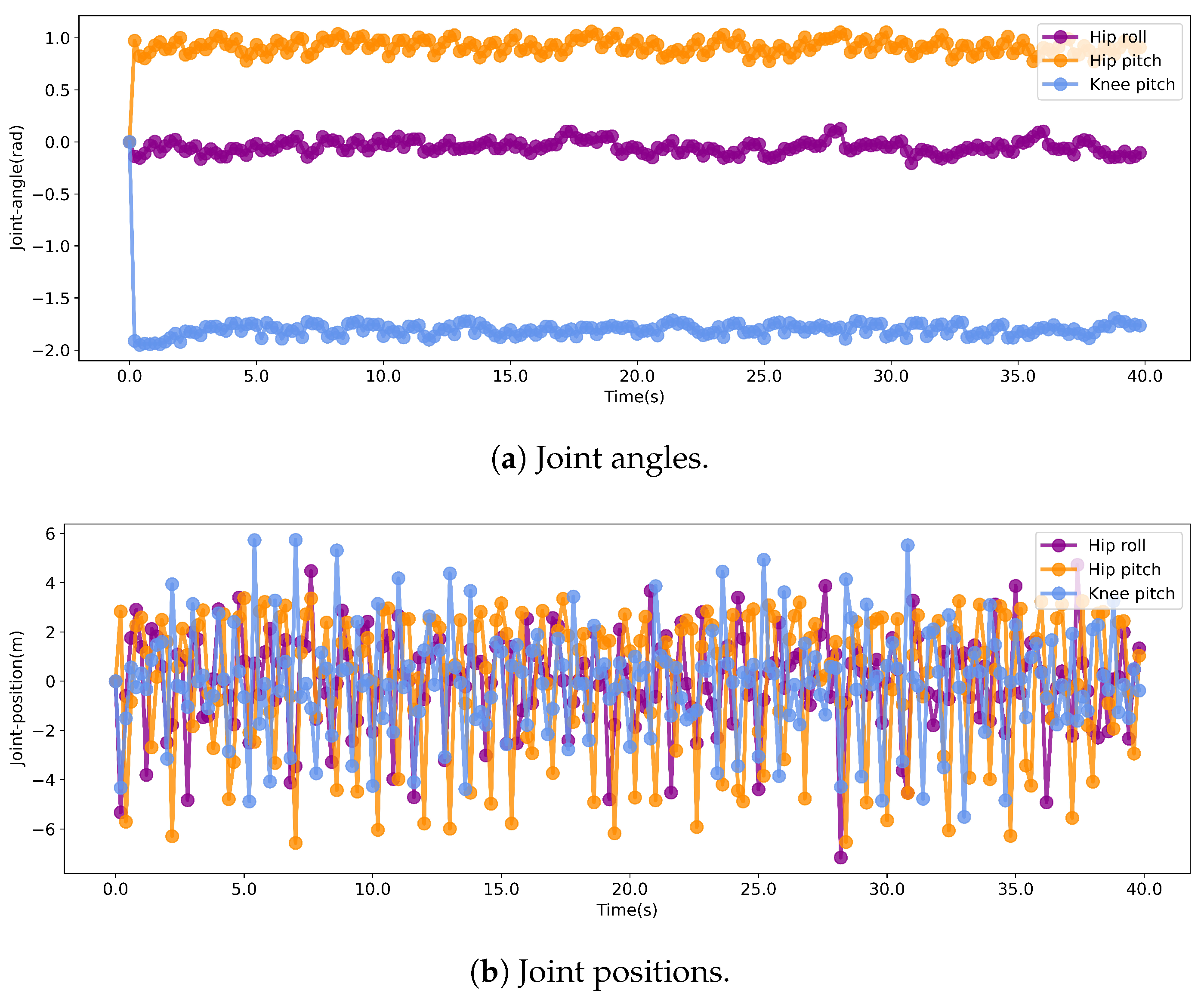
The time-series movements of the left front leg joint angle and joint position are shown in Figure 15a and Figure 15b, respectively. Our designed reward function and constraints do not include any periodic settings; therefore, the leg movements of the trained robot exhibit aperiodic motions. The time series of joint angles and joint positions are consistent with those in Figure 14, both starting from the robot setup. In addition, we have added the comparative leg movements of SAC, as shown in Figure 16a,b. The motion patterns of other reinforcement learning methods are similar to that of the proposed method, all exhibiting irregular movements.

We tested the performance under different reward conditions. In the new comparative tests, we added the energy consumption of the motor to the reward function. The new reward function can be defined as

$${\mathit{R}}_t=\alpha ({\mathit{X}}_1\left(t\right)-{\mathit{X}}_1(t-1))-\beta \left(\mathit{P}\right),$$

(22)

where $\alpha$ and $\beta$ are, respectively, the coefficients of the forward velocity and energy consumption. Energy consumption $\mathit{P}$ is defined as

$$\mathit{P}={\sum }_{i=i}^n(t_i\ast v_i),$$

(23)

where t and v are torque and angular velocity, respectively.

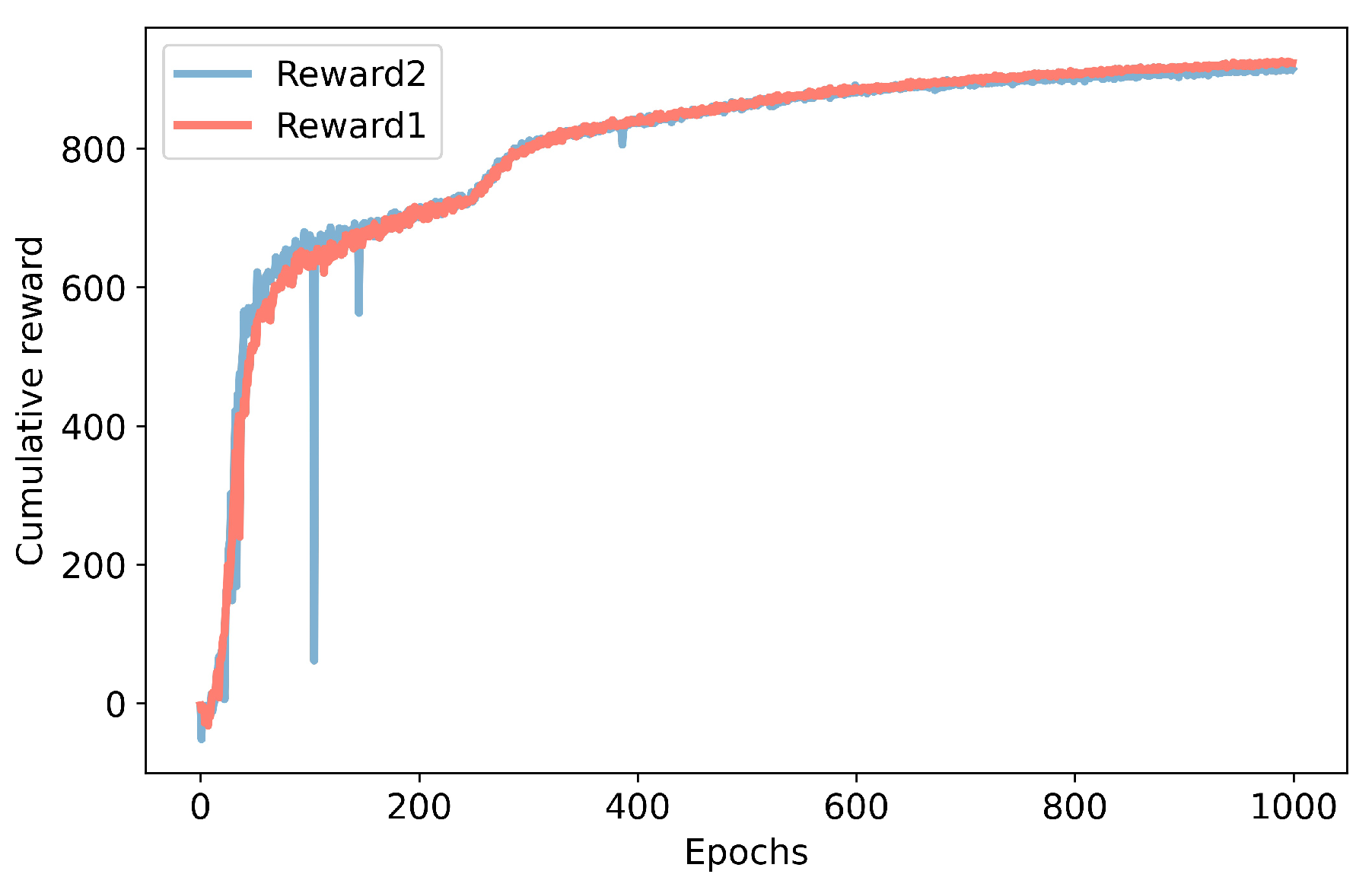
The results of cumulative training rewards for different reward functions are shown in Figure 17, and the test results of speed and energy consumption on different terrains are shown in Figure 18 and Figure 19. In the experiments, $\alpha =1$ and $\beta =-0.1$.

In the figure, Reward 1 refers to the original reward function, and Reward 2 refers to the reward function with added energy consumption. The final training rewards using Reward 1 and Reward 2 are 923 and 914, respectively. After adopting the new reward function, the energy consumption on the three terrains has decreased significantly; however, the test speed has decayed severely on sloped terrain and real-world terrain.

5. Conclusions

In this paper, we proposed a HTS-SAC method to optimize locomotion policy from historical time-series data. We designed four mutual information decision conditions based on the k-nearest neighbor mutual information theory. Through the decision conditions analysis of the correlation, the key feature variables affecting the locomotion performance were obtained. Then, we designed a heterogeneous time-series neural network to learn the high-level features from the key feature variables and designed the HTS-SAC algorithm to learn the enhanced policy. The simulation results show that the HTS-SAC can generate better policy and provide faster speed on various terrains.

The DRL-based methods do not require a complex and exact model of the unmanned quadruped robots and can be widely applied to various complex scenarios through learning and training with a lot of interaction data. However, the DRL-based methods require a lot of high-quality and diverse data to cover all the possible application scenarios. In addition, how to transfer the learned model and strategy into real robot hardware with a safety guarantee is also necessary. This makes it a great challenge to deploy the DRL-based methods in real-world systems. In future research, we will analyze the stability and implementation of the proposed method through more in-depth theoretical research and more comprehensive hardware experiments.

The proposed method is an end-to-end, data-driven reinforcement learning approach that does not rely on the robot’s model and has scalability. Quadruped robots and unmanned aerial vehicles (UAVs) both belong to unmanned robotic systems. When UAVs are adopted, information such as the UAV’s attitude, position, velocity, and surrounding environment can be collected. Through the learning and training of the model, the UAV can formulate control strategies for each motor by perceiving its current state, thereby achieving control of the UAV.