PowerLine-MTYOLO: A Multitask YOLO Model for Simultaneous Cable Segmentation and Broken Strand Detection

Abstract

Power transmission infrastructure requires continuous inspection to prevent failures and ensure grid stability. UAV-based systems, enhanced with deep learning, have emerged as an efficient alternative to traditional, labor-intensive inspection methods. However, most existing approaches rely on separate models for cable segmentation and anomaly detection, leading to increased computational overhead and reduced reliability in real-time applications. To address these limitations, we propose PowerLine-MTYOLO, a lightweight, one-stage, multitask model designed for simultaneous power cable segmentation and broken strand detection from UAV imagery. Built upon the A-YOLOM architecture, and leveraging the YOLOv8 foundation, our model introduces four novel specialized modules—SDPM, HAD, EFR, and the Shape-Aware Wise IoU loss—that improve geometric understanding, structural consistency, and bounding-box precision. We also present the Merged Public Power Cable Dataset (MPCD), a diverse, open-source dataset tailored for multitask training and evaluation. The experimental results show that our model achieves up to +10.68% mAP@50 and +1.7% IoU compared to A-YOLOM, while also outperforming recent YOLO-based detectors in both accuracy and efficiency. These gains are achieved with a smaller model memory footprint and a similar inference speed compared to A-YOLOM. By unifying detection and segmentation into a single framework, PowerLine-MTYOLO offers a promising solution for autonomous aerial inspection and lays the groundwork for future advances in fine-structure monitoring tasks.

1. Introduction

The inspection and maintenance of power transmission infrastructure are critical for ensuring grid reliability and preventing failures that can lead to blackouts or hazardous conditions. Traditional inspection methods rely on ground-based visual checks or manned aerial surveys, both of which are expensive, time-consuming, and pose safety risks [1]. In recent years, unmanned aerial vehicles (UAVs) equipped with computer vision systems have emerged as an efficient alternative, offering autonomous and real-time monitoring of power lines and their components [2,3]. These UAV-based inspection systems leverage deep learning algorithms to automate defect detection, reducing manual effort and significantly improving efficiency.

Among the various computer vision tasks involved in UAV-based power line inspection, cable segmentation and broken strand detection stand out as fundamental operations. Cable segmentation serves as a critical first step, enabling the precise localization of the power line’s geometry and helping define regions of interest (ROIs) for subsequent analysis. This is particularly important for UAV navigation, infrastructure modeling, and accurate localization of potential defects. Among such anomalies, broken strands—partial fractures or unraveling of the cable’s wire filaments—represent subtle but serious defects that can compromise mechanical integrity or pose safety hazards.

Despite their close operational relevance, most existing works treat them as distinct tasks, designing models that address only one objective at a time. For instance, prior studies on power cable segmentation have primarily focused on isolating cable structures to support UAV navigation or infrastructure mapping, without addressing downstream defect detection tasks [4,5,6,7,8,9]. Conversely, several recent approaches aimed solely at detecting cable anomalies, such as broken strands, using object detection or classification models applied to cropped regions or full-frame images [10,11,12,13]. These two lines of work, though complementary, remain largely disconnected, resulting in suboptimal performance when deployed in end-to-end inspection pipelines.

In the few cases where both are considered [14], they are implemented in a sequential fashion—typically applying a segmentation model first, followed by a separate model for defect detection (as illustrated in Figure 1). While this approach can be effective, it introduces two key limitations: (1) error propagation, where inaccurate segmentation undermines the subsequent detection stage; and (2) increased inference latency, due to the computational overhead of running multiple models—an issue that is particularly problematic for real-time UAV-based deployment.

To address these limitations, recent research has explored multitask learning (MTL) to integrate multiple vision tasks into a single model, thereby improving efficiency and robustness [15,16]. In other fields, such as medical imaging or autonomous driving, MTL has demonstrated its ability to enhance performance by leveraging shared feature representations across tasks [17,18,19,20]. However, in the specific domain of UAV-based power line inspection, most studies still follow the sequential paradigm, and multitask architectures remain largely unexplored, as previously mentioned.

To this end, we propose a one-stage multitask YOLO-based model that simultaneously performs power line segmentation and broken strand detection within a single inference pipeline. Inspired by the recently introduced A-YOLOM framework [21], our model eliminates the need for separate segmentation and detection steps, reducing computational complexity and enhancing real-time applicability for UAV-based inspection missions. To validate our approach, we constructed a dedicated dataset containing annotated power line segments and anomalies, ensuring a comprehensive evaluation under diverse environmental conditions. Our experimental results demonstrate that the proposed model achieves state-of-the-art performance in both segmentation and anomaly detection tasks while maintaining real-time processing speed suitable for UAV deployment.

The main contributions of this work are as follows:

• We propose PowerLine-MTYOLO, a novel multitask YOLO-based architecture that performs simultaneous cable segmentation and anomaly detection (specifically, broken strand localization) in a single-stage framework.
• We construct and release the Merged Public Power Cable Dataset (MPCD), a curated benchmark that includes fine-grained annotations for both segmentation and detection tasks, addressing the current lack of multitask datasets in this domain.

2. Materials and Methods

2.1. Introduction to A-YOLOM

Deep learning-based multitask models have gained increasing attention due to their ability to improve computational efficiency and resource allocation, particularly in time-sensitive applications such as autonomous systems and aerial surveillance. A-YOLOM (Adaptive You Only Look Once for Multi-Task Learning) was introduced as a lightweight, real-time, and adaptive model that integrates multiple vision tasks within a single framework. Originally developed for autonomous driving applications, A-YOLOM is designed to perform object detection, drivable area segmentation, and lane line segmentation simultaneously, eliminating the need for separate models for each task.

Built upon the YOLOv8 architecture, A-YOLOM introduces several key modifications to facilitate multitask learning while preserving high-speed inference. A-YOLOM employs a single shared backbone to extract multi-scale features, which are then processed by two distinct network branches. The detection branch utilizes a Path Aggregation Network (PAN) to enhance spatial and contextual awareness, whereas the segmentation branch incorporates a Feature Pyramid Network (FPN) to improve feature extraction for segmentation tasks. At the final stage, the network includes two task-specific heads: the detection head, responsible for predicting bounding boxes and classification scores; and the segmentation head, which generates pixel-wise segmentation masks for drivable areas and lane markings.

A-YOLOM’s training process is optimized through a multitask loss function that combines detection and segmentation objectives in a single end-to-end learning framework. The detection loss function integrates Binary Cross-Entropy (BCE) loss, Distribution Focal Loss (DFL), and Complete IoU (CIoU) loss to enhance object classification and bounding-box localization. Simultaneously, segmentation loss is computed using a combination of Focal Loss (FL) and Tversky Loss (TL) to improve pixel-wise classification accuracy while addressing imbalanced data distributions. The total training objective is formulated as follows:

$$L_{\mathrm{total}}=L_{\det }+L_{{\mathrm{seg}}_{\mathrm{drivable} \mathrm{area}}}+L_{{\mathrm{seg}}_{\mathrm{lane} \mathrm{line}}}$$

(1)

where $L_{\det }$ represents the detection loss, while $L_{\mathrm{seg}}$ corresponds to the segmentation loss for both drivable areas and lane markings. During training, the model undergoes backpropagation-based optimization, where the computed loss gradients are propagated backward to update the model parameters. Optimization is performed using either Stochastic Gradient Descent or the Adam optimizer, following a learning rate annealing strategy that facilitates rapid convergence during the early training phases and fine-tuning in the later stages.

Experimental evaluations conducted on the BDD100K dataset demonstrated A-YOLOM’s superior performance across multiple vision tasks, achieving an mAP@50 of 81.1% for object detection, mIoU of 91.0% for drivable area segmentation, and an IoU of 28.8% for lane line segmentation. Compared to conventional multitask models such as YOLOP and MultiNet, A-YOLOM achieves improved accuracy while maintaining low latency. These results establish A-YOLOM as a state-of-the-art (SOTA) multitask framework in real-time perception scenarios.

While A-YOLOM was originally developed for autonomous driving, its efficient architecture and real-time inference capability make it highly suitable for UAV-based power line inspection. Drawing on this foundation, we propose PowerLine-MTYOLO.

2.2. Our Model: PowerLine-MTYOLO

2.2.1. Motivation and Design Principles

While A-YOLOM provides a strong foundation for multitask perception, its design was not specifically optimized for power line cable segmentation and the detection of broken strands. Power lines exhibit distinct structural and visual characteristics, including their thin, elongated shapes and the often-subtle nature of defects such as fractured strands. These properties make segmentation and anomaly detection significantly more challenging than conventional object detection tasks, where objects typically have well-defined edges and larger surface areas.

PowerLine-MTYOLO was developed to address these unique challenges by introducing specialized architectural modifications that enhance both segmentation and defect detection. Given that small-scale structural anomalies along cables require high localization precision, our model integrates a refined detection head to improve feature extraction for defect identification. Moreover, traditional segmentation architectures often struggle to maintain the continuity of thin structures, resulting in fragmented predictions. To resolve this, we incorporated a segmentation head with an edge-aware refinement mechanism, specifically designed to preserve fine details and maintain the structural integrity of power line cables.

Beyond task-specific improvements, PowerLine-MTYOLO replaces conventional max pooling-based feature extraction with a more adaptable multi-scale feature learning approach. This modification enables the model to capture both fine-grained local features and global contextual information, leading to more stable segmentation masks and more precise defect localization. In addition, we introduce the Shape-Aware Wise IoU loss, tailored to the elongated structure of power lines, to improve bounding-box regression and defect detection accuracy.

These enhancements make PowerLine-MTYOLO a highly specialized multitask model for UAV-based power line inspection.

2.2.2. Network Architecture

The PowerLine-MTYOLO framework is designed for simultaneous power line segmentation and defect detection, processing a single input image and producing two outputs—one for segmentation and another for object detection. While these two branches operate independently at inference time, their joint training confers multiple benefits. First, the segmentation task reinforces the model’s spatial understanding of cable structures, which indirectly enhances the quality of features shared with the detection branch, leading to more accurate anomaly localization (as shown in Section 3.2). This is particularly relevant, since both tasks focus on the same physical component (the cable), albeit in different states (normal vs. defective). Conversely, the anomaly detection branch also benefits from the segmentation process. Learning to detect localized defects sharpens the model’s attention on critical regions—often near cable boundaries—thereby improving the segmentation precision and reducing confusion with background elements. This reciprocal learning mechanism encourages a richer and more discriminative feature space. Second, although segmentation is not directly involved for anomaly detection during inference, it remains crucial for many practical UAV-based applications. For instance, segmentation maps can support autonomous navigation by enabling a drone to follow the cable path in real time, while simultaneously detecting anomalies. This dual-output design therefore provides both technical synergy and operational flexibility.

As illustrated in Figure 2, the model structure follows the general layout of A-YOLOM, with key modifications tailored for power line inspection.

The input image, with dimensions of 640 × 640 × 3, is first processed by the backbone (see Figure 2, top), which progressively extracts multi-scale features through a cascade of convolutional and residual blocks. Specifically, the image passes through successive Conv → C2f layers with increasing channel depths and downsampling strides, enabling the model to capture both low-level spatial textures and high-level semantic structures. Each Conv block consists of a convolutional layer followed by batch normalization and a SiLU activation function. These operations yield feature maps at five spatial resolutions (P1 to P5), where P5 corresponds to the deepest layer with the smallest spatial resolution and highest semantic abstraction. At the deepest level (P5), we replace the original SPPF block from YOLOv8 with our custom Shared Dilation Pyramid Module (SDPM). This module increases the effective receptive field by applying multiple depthwise separable convolutions with different dilation rates, thereby enriching the feature representations without adding substantial computational burden. This replacement is highlighted in yellow in Figure 2, just above the backbone’s output.

Once extracted, the multi-scale features are distributed into two distinct necks: a detection path on the left and a segmentation path on the right. The detection branch follows the classical PANet-style neck architecture adopted by YOLOv8, designed to promote rich multi-scale feature fusion across shallow and deep layers. The process begins with upsampling operations (e.g., P5 → P4, P4 → P3), which are applied to align the spatial resolutions of deep feature maps with those from earlier stages of the backbone. This alignment is crucial to enable the concatenation of semantically rich (deep) features with spatially precise (shallow) ones. Upsampling does not add new information per se, but it ensures that all feature maps involved in the fusion share the same spatial dimensions. After concatenation, each fused output undergoes a C2f refinement block, which allows the network to reprocess and compress the combined features, improving both representation power and computational efficiency. These refined feature maps are then downsampled again (e.g., P3 → P4, P4 → P5) using strided convolutions. This downsampling serves not only to restore deeper resolutions but also to ensure bidirectional flow of information, making it possible to capture both fine details from shallow layers and semantic abstractions from deep ones. This process yields a hierarchically aggregated feature space, where object features of varying sizes and complexities are coherently integrated. Finally, these multi-scale representations (from P3, P4, and P5) are passed to the Hierarchical Attention Detection (HAD) head, which performs bounding-box regression and object classification. By operating at multiple resolutions, the detection head is inherently more robust to variations in object size, shape, and context—particularly relevant in UAV-based inspection, where defects may appear at any scale.

In parallel, the segmentation branch adopts a decoder-style architecture, mirroring the feature aggregation logic but focused on spatial reconstruction. Starting from the deepest level (P5), it performs progressive upsampling (P5 → P1) and integrates skip connections from corresponding backbone outputs (P4, P3, …, P1), preserving high-resolution spatial cues throughout the decoding process. Each upsampled and fused stage is refined by a C2f block, improving spatial coherence and suppressing artifacts. In addition, the segmentation neck uniquely leverages the adaptive concatenation module [21] inherited from A-YOLOM, which enables dynamic feature aggregation during training. Rather than systematically merging feature maps from skip connections and the main path, this module applies a sigmoid-activated gating mechanism to decide whether the auxiliary input should be concatenated. If the gate is inactive, only the main branch is propagated; otherwise, the concatenated tensor is compressed via a 1 × 1 convolution. This selective fusion process is repeated throughout the segmentation pathway, as shown by the “Adaptive Concat” blocks in Figure 2. It effectively acts as a form of learnable dropout, allowing the network to suppress noisy or redundant spatial information and enhancing the robustness of the segmentation output. This refined multi-scale path is then directed to the Edge-Enhanced Refinement (EFR-Seg) head, which specializes in reconstructing cable masks with high boundary fidelity and structural consistency.

This dual-neck configuration allows the model to simultaneously exploit shared backbone features for detection and segmentation, while tailoring each branch to the specific spatial and semantic demands of its task.

During training, both branches are supervised simultaneously using their respective loss functions. These losses are backpropagated jointly through the necks and the shared backbone, allowing the model to optimize feature representations that serve both tasks. This multi-objective learning encourages the network to extract spatially precise features (helpful for segmentation) while also being sensitive to localized anomalies (critical for detection).

Additional technical details and the design of our novel modules introduced in PowerLine-MTYOLO are discussed in the following sections.

• Shared Dilation Pyramid Module (SDPM):

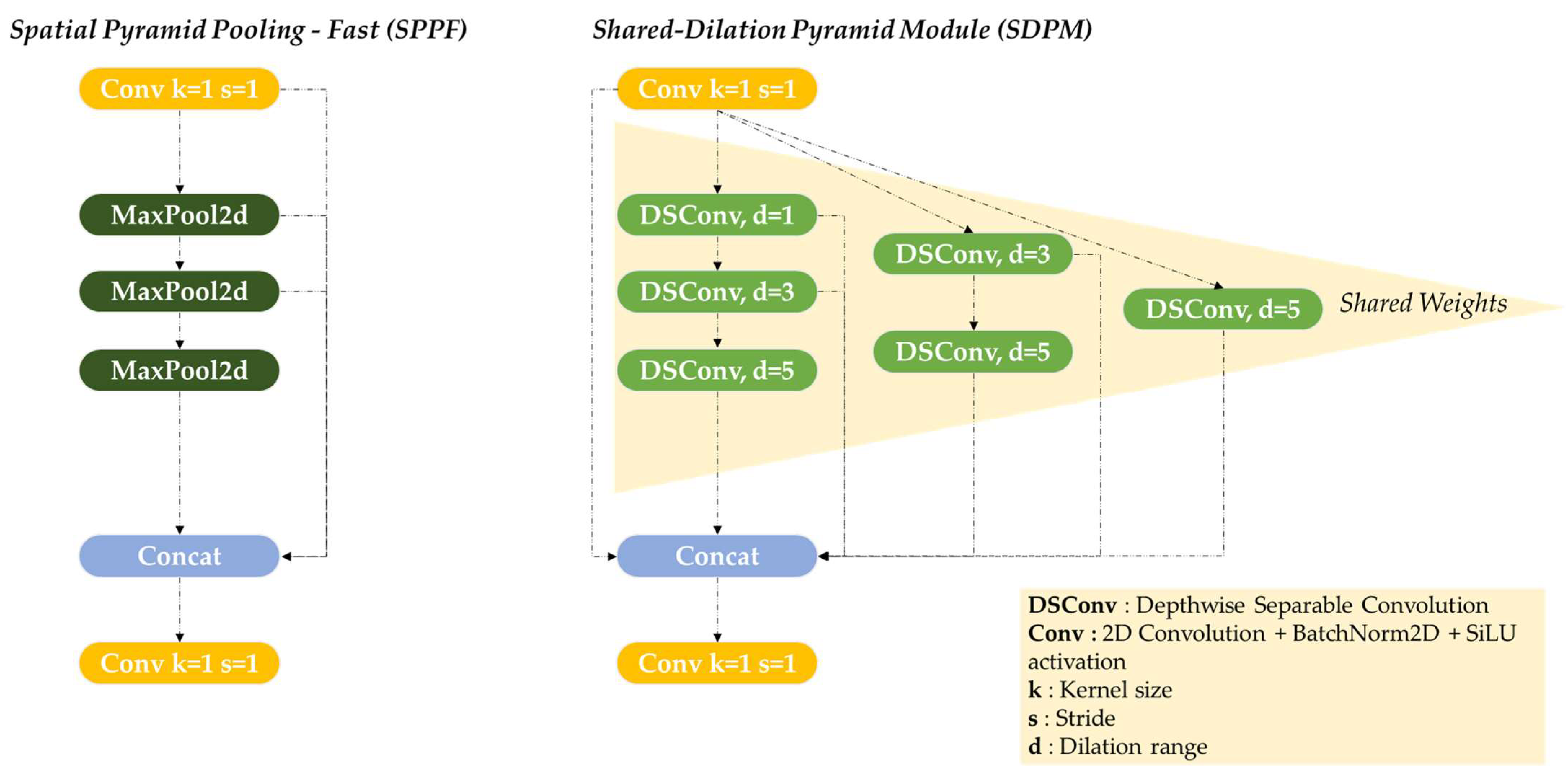
Feature extraction is a crucial step in power line segmentation and broken strand detection, where maintaining structural continuity is essential. Traditional approaches, such as Spatial Pyramid Pooling-Fast (SPPF), rely on max pooling to extract multi-scale features.

However, max pooling removes fine spatial details, which can disrupt the segmentation of thin and elongated structures like power lines. To address this limitation, we introduce the Shared Dilation Pyramid Module (SDPM), illustrated in Figure 3, which replaces SPPF with a dilation-based multi-path approach tailored to the characteristics of power lines.

The SDPM is designed to capture both fine details and large-scale contextual information by leveraging depthwise separable convolutions (DSConv) [22] with increasing dilation rates and a kernel size of 3 (as explained in Figure 4).

Since power lines are long structures in images, effective segmentation requires not only local precision but also an extended receptive field to understand the broader context. Dilated convolutions enable this expansion, where a small dilation rate focuses on capturing local fine details, while larger dilation rates progressively explore a wider spatial context, ensuring that the network can model the continuity of long cables effectively. To achieve this, the SDPM follows a three-path hierarchical structure with residual connections. Each path extracts features at different scales, ensuring a progressive increase in receptive field without losing critical information.

The first path starts with a small dilation (d = 1), preserving local details before progressively increasing dilation (d = 3, 5). The second path begins at d = 3, capturing intermediate-scale structures before reaching d = 5 to integrate broader context. The third path processes features at d = 5 from the outset, ensuring that long-range dependencies are incorporated early in the feature extraction process. This structured expansion allows the model to match the elongated nature of power lines, ensuring both precise segmentation and contextual continuity. Also, residual connections are integrated across paths, allowing feature information from earlier dilation stages to be retained as the receptive field expands. These connections help mitigate feature degradation, ensuring that finer details are not lost in deeper layers.

In addition to its hierarchical structure, the SDPM employs a shared-weight convolutional mechanism, which reduces redundancy while preserving a diverse range of spatial features. Instead of using separate convolutional kernels for each dilation level, the SDPM shares parameters across different receptive fields, resulting in a more lightweight and efficient representation. In our implementation, the shared-weight mechanism consists of applying the same depthwise convolution kernel across multiple dilation levels using F.conv2d, with a fixed weight tensor shared among paths. The reference kernel used for sharing is the base depthwise convolution filter (not the point-wise convolution; see Figure 4). For example, for dilation rates 1, 3, and 5, the same filter W is reused at different scales: F.conv2d (input, weight = W, dilation = d). This design enables efficient multi-scale feature extraction without introducing redundant parameters. Finally, the extracted multi-scale features are concatenated and refined through a final 1 × 1 convolution block (Conv2D + BatchNorm + SiLU), which ensures smooth feature integration before passing them to the neck.

2.

Edge-Enhanced Refinement (EFR-Seg) Head:

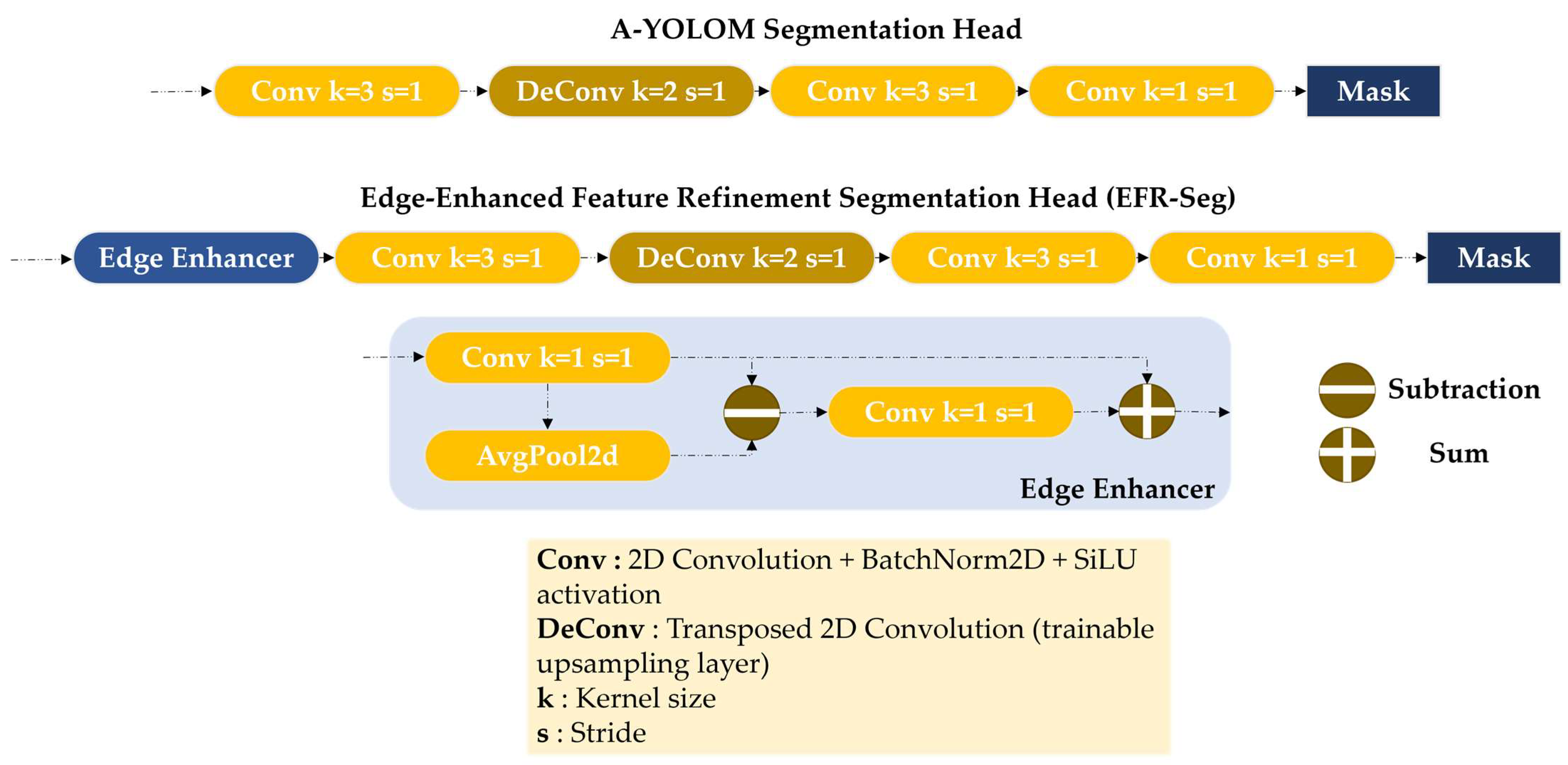
Accurate power line segmentation is a challenging task due to the thin, elongated nature of cables, which can be difficult to distinguish from the background. In prior architectures, A-YOLOM’s segmentation head provided a lightweight approach to mask generation but lacked specialized mechanisms for enhancing edge precision. To address this, we introduce the Edge-Enhanced Refinement (EFR) segmentation head, illustrated in Figure 5, which retains the efficiency of the original A-YOLOM segmentation head while integrating an Edge Enhancer block at the input to refine boundary information.

The primary goal of the EFR segmentation head is to improve edge awareness in power line segmentation without significantly increasing the computational complexity. Traditional edge detection techniques, such as Sobel filters [23] or gradient-based methods [24], explicitly compute edges but often suffer from noise sensitivity and are not inherently trainable within deep networks. Instead of using such conventional methods, we introduce an Edge Enhancer module, which learns edge-aware features in a pixel-wise manner using trainable convolutions. That said, several recent strategies have indeed sought to embed edge awareness within deep learning pipelines using trainable modules. Notably, works such as HED [25], PiDiNet [26], and AERNet [27] propose learnable edge refinement mechanisms, often based on multi-scale side outputs, deep supervision, or attention-based decoding blocks.

While these methods achieve strong results, they tend to introduce considerable architectural complexity and parameter overhead. In contrast, our design deliberately emphasizes simplicity, efficiency, and seamless integration, as it relies solely on an average pooling operation and two lightweight 1 × 1 convolutions. Moreover, in Section 3.6, we conduct a comparative ablation against several of these strategies—including both non-learnable and learnable alternatives—to support this discussion.

The core purpose of the Edge Enhancer module is to function as a lightweight, learnable edge detector by isolating high-frequency components within the feature map and amplifying boundary-specific signals to support downstream segmentation. Importantly, the design philosophy behind this module is not to replace or suppress the original features but to softly enrich them. It preserves the full semantic content of the input and selectively adds edge-focused cues on top. As a result, even if the added signal is not perfectly accurate, the underlying information remains unaffected, making the enhancer non-destructive, safe, and effective in guiding the network’s attention toward fine structures such as thin cables.

Placing the Edge Enhancer at the entry point of the segmentation branch encourages the network to learn edge sensitivity from the earliest layers, reinforcing contour features throughout the entire mask generation process.

Specifically, as shown in Figure 5 and Figure 6, the Edge Enhancer module is defined by the following operations:

• 1 × 1 Convolution: A point-wise convolution is applied to extract localized features from each pixel independently. This operation preserves spatial granularity and highlights local activations that are potentially associated with edges, analogous to examining the intensity of individual pixels without blending adjacent information. As illustrated in Figure 6 (image #1), this step emphasizes signal contrast in localized regions, especially around cable discontinuities.
• 3 × 3 Average Pooling: The output is then passed through an average pooling layer to produce a smoothed version of the feature map. Compared to max pooling, average pooling is less sensitive to noise and better at capturing broad contextual patterns. Conceptually, this acts like applying a soft-focus lens, suppressing fine details while retaining low-frequency background structures. This smoothing effect is visualized in Figure 6 (image #2), where high-frequency noise is reduced, leaving a softened contour representation. To ensure shape compatibility during the subtraction, we apply a 3 × 3 average pooling operation with stride = 1 and padding = 1, which maintains the same spatial resolution as the input. While pooling operations are typically used to reduce spatial dimensions, in this case, it serves as a smoothing filter to extract low-frequency components without altering the feature map size.
• Subtraction Operation: The smoothed feature map is subtracted from the original point-wise features, isolating high-frequency content where significant changes occur. These differences typically correspond to edges or transitions, effectively functioning as a trainable edge extractor. As shown in Figure 6 (image #3), the difference map clearly highlights structural discontinuities such as broken cable strands and object contours.
• Sigmoid-Activated Convolution: A subsequent convolution layer followed by a sigmoid activation refines the edge map. The sigmoid non-linearity scales responses between 0 and 1, allowing the network to softly highlight important edge features. In this context, the sigmoid output acts as a soft attention mask, where values closer to 1 indicate a high likelihood of edge presence (e.g., cable boundary), while values near 0 suggest non-edge or background regions. This enables the model to emphasize relevant contours without applying rigid thresholds, promoting smooth and adaptive boundary refinement. This refined edge mask is presented in Figure 6 (image #4), where enhanced contours begin to emerge. However, since this visualization is produced by applying the Edge Enhancer only once, without any training, the convolutional layer has not yet learned to distinguish cable-specific boundaries from other visual transitions. As a result, the highlighted edges include both relevant and irrelevant structures (like vegetation), illustrating the raw potential of the module prior to task-specific learning.
• Residual Addition: Finally, the refined edge response is added back to the original input, preserving the semantic richness of the features while amplifying their edge-localized characteristics. As shown in Figure 6 (image #5), the edge-focused information appears in pink when overlaid on the original RGB image, providing a clear visualization of the enhancement effect.

The enhanced feature map is then passed through a lightweight yet effective decoding pipeline to produce the final binary segmentation mask. First, the Edge Enhancer output is processed by a 3 × 3 convolution block with stride = 1 (i.e., without spatial downsampling), which extracts a compact set of semantic features while preserving spatial detail. This is followed by a transpose convolution layer (also known as deconvolution), which upsamples the feature map by a factor of 2 while learning how to reconstruct higher-resolution structures. Compared to naïve interpolation (e.g., bilinear), transpose convolution learns trainable filters for upsampling, enabling it to better preserve edge alignment and structure—particularly beneficial for thin cables. Next, another 3 × 3 convolution block is applied to refine the upsampled features and enhance spatial consistency. Finally, the output is passed through a 1 × 1 convolution block that reduces the channel dimensions to match the number of segmentation classes (typically two: cable vs. background). The resulting activation map is then passed through a sigmoid function to obtain a probability mask.

3.

Hierarchical Attention Detection (HAD) Head:

Anomaly detection in power line inspection requires an efficient yet accurate prediction head to jointly estimate bounding boxes and classify objects while maintaining computational efficiency. Traditional architectures, such as A-YOLOM, rely on separate branches for classification and bounding-box regression. While independent processing improves specialization, it significantly increases the computational cost and memory consumption, making it less suitable for real-time applications such as UAV-based power line monitoring. To address this limitation, we introduce the Hierarchical Attention Detection (HAD) head, as illustrated in Figure 7, which replaces the original detection head in A-YOLOM.

The key motivation behind the HAD head is parameter reduction through branch fusion. By merging the classification and bounding-box branches, HAD minimizes redundant computations, resulting in a lighter architecture with fewer parameters. Unlike A-YOLOM, which uses two entirely separate sub-networks for classification and bounding-box regression, our model leverages a shared feature extraction stage (Hierarchical Attention Bottleneck) that outputs a unified feature map. This shared feature map is then passed through two lightweight, parallel 1 × 1 convolutional layers—one for class prediction and one for bounding-box offset regression—which operate on the same input. This architectural choice drastically reduces computational redundancy, as both tasks utilize the same underlying features, and the branching only occurs at the final convolutional stage. Furthermore, the predictions are concatenated along the channel dimension before decoding, eliminating the need for separate spatial feature flows. In other words, unlike A-YOLOM, where the detection head (Figure 7, top) processes the same input features through two entirely different branches (each with its own intermediate layers, including four convolutional layers with a kernel size of 3, resulting in a significantly higher number of parameters), our approach avoids this duplication, saving parameters and computation while preserving prediction quality. However, this fusion presents a significant challenge: combining these two tasks can degrade accuracy, as bounding-box regression and classification require distinct feature representations. To mitigate this issue, HAD introduces a Hierarchical Attention Bottleneck (HAB), which enhances feature expressiveness by selectively refining spatial and channel-wise information.

Inspired by the Shared Dilation Pyramid Module (SDPM), HAD utilizes DSConv with sequential dilations to process multi-scale contextual features efficiently. Instead of handling dilation separately at different stages, HAD follows a progressive dilation strategy with shared weights, allowing the model to capture fine details while gradually expanding the receptive field.

To further improve feature selection, we integrate Squeeze-and-Excitation (SE) attention [28] after each DSConv operation. While DSConv primarily focuses on spatial feature refinement, the introduction of SE attention mechanisms ensures that the model also prioritizes critical channel-wise information. This is particularly important in deep neural networks, where a large number of feature maps are generated near the final layers. By dynamically reweighting the channel responses, SE attention helps compensate for the potential loss of discriminative information caused by branch fusion.

Specifically, as shown in Figure 7, the HAD head follows a carefully designed sequence of operations to jointly produce bounding-box and classification predictions in an efficient manner. It starts with a 1 × 1 convolutional projection layer that reduces the number of channels and standardizes feature representations, ensuring a compact and normalized input space for subsequent processing.

The transformed features then pass through the HAB, which forms the core of the HAD head. This module applies a sequence of three depthwise separable convolutions (DSConv), each with a kernel size of 3 × 3, and progressively increasing dilation rates of 1, 3, and 5, respectively. This strategy allows the network to extract both fine-grained and large-scale contextual information while maintaining a low parameter count. Importantly, the convolutional weights are shared across dilation levels, enhancing computational efficiency and ensuring consistent feature encoding across different receptive fields.

After each DSConv block, the features are refined through a Squeeze-and-Excitation (SE) attention module. Each SE block uses a reduction ratio of 16, implemented via two 1 × 1 convolutions: the first reduces the number of channels, and the second restores it, followed by a sigmoid gating function. This mechanism dynamically reweights the feature channels based on their global relevance, reinforcing the most informative components while suppressing less relevant ones.

In the final stage, the attention-enhanced features are passed through two parallel 1 × 1 convolutions—one head predicts the class probabilities, and the other outputs the bounding-box offsets. These predictions are concatenated and post-processed using specialized loss functions: bounding-box regression is supervised using our proposed Shape-Aware Wise IoU loss, enhanced with Distribution Focal Loss (DFL) for finer localization, while Binary Cross-Entropy (BCE) is used for classification supervision. The formulation and rationale of these loss functions are further explained in the next section.

2.2.3. Loss Functions

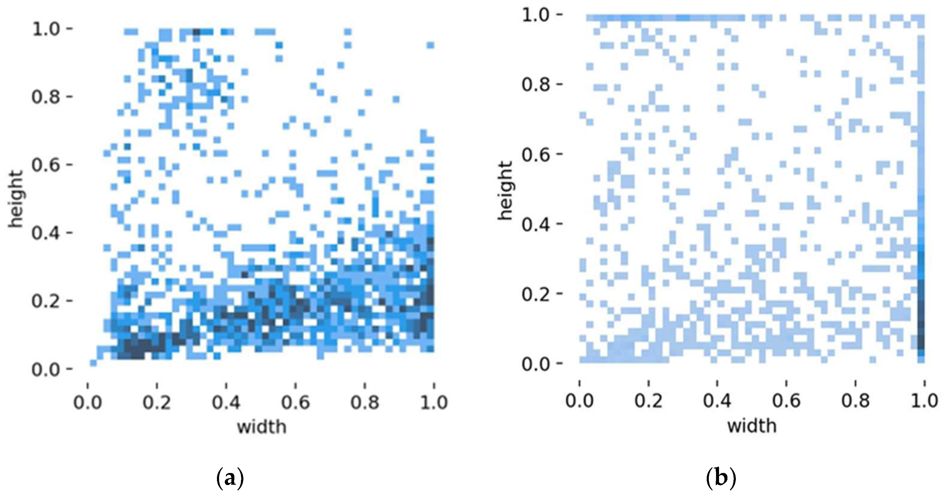
Accurate bounding-box regression is crucial for detecting broken strands and cable anomalies in power line inspection. To evaluate the quality of a predicted bounding box, most modern detectors rely on the Intersection-over-Union (IoU) metric, which measures the ratio of the overlapping area to the union area between the predicted and ground-truth boxes. A higher IoU score indicates better alignment and coverage, and this metric serves as the basis for many loss functions in object detection. Traditional IoU-based loss functions, such as CIoU and DIoU, primarily optimize for overlap and center distance alignment but do not account for shape differences explicitly. This limitation becomes particularly problematic in power line defect detection, where defects exhibit high aspect ratio variations (refer to the Section 2.3). Such variations make it difficult for standard IoU losses to properly guide the model in refining bounding-box predictions, leading to misaligned or imprecise bounding boxes around defects.

To address these challenges, we introduce the Shape-Aware Wise IoU loss, which builds upon Shape IoU [29] by integrating adaptive scaling mechanisms from Wise IoU [30]. This formulation aims to enhance the model’s ability to capture elongated structures while maintaining stable gradient flow for optimization. Shape IoU extends traditional IoU by introducing a shape distance term and a shape-aware penalty function, ensuring that the bounding boxes align not only in position but also in aspect ratio, making it more suited for objects with non-uniform shapes such as cables or broken strands. However, Shape IoU alone is insufficient, as its static penalty structure does not adapt to dynamic localization challenges during training. For instance, broken cables are often small, thin, and partially occluded, making their appearance highly variable across scenes. In such cases, a fixed penalty may either under-emphasize subtle misalignments or overly penalize reasonable predictions, leading to unstable convergence. By integrating the adaptive focusing mechanism from Wise IoU, our Shape-Aware Wise IoU loss dynamically adjusts the penalty strength based on the confidence and quality of the prediction—encouraging tighter localization when the model is confident, and being more forgiving when uncertainty is high. In summary, this approach can be likened to fitting a custom-shaped sticker onto an object: traditional IoU focuses on ensuring that the sticker is centered and covers most of the surface, whereas Shape-Aware Wise IoU ensures that the sticker also matches the object’s shape—whether long and narrow or square. The “wise” part adapts how strictly the fit is judged, depending on how difficult the object is to locate.

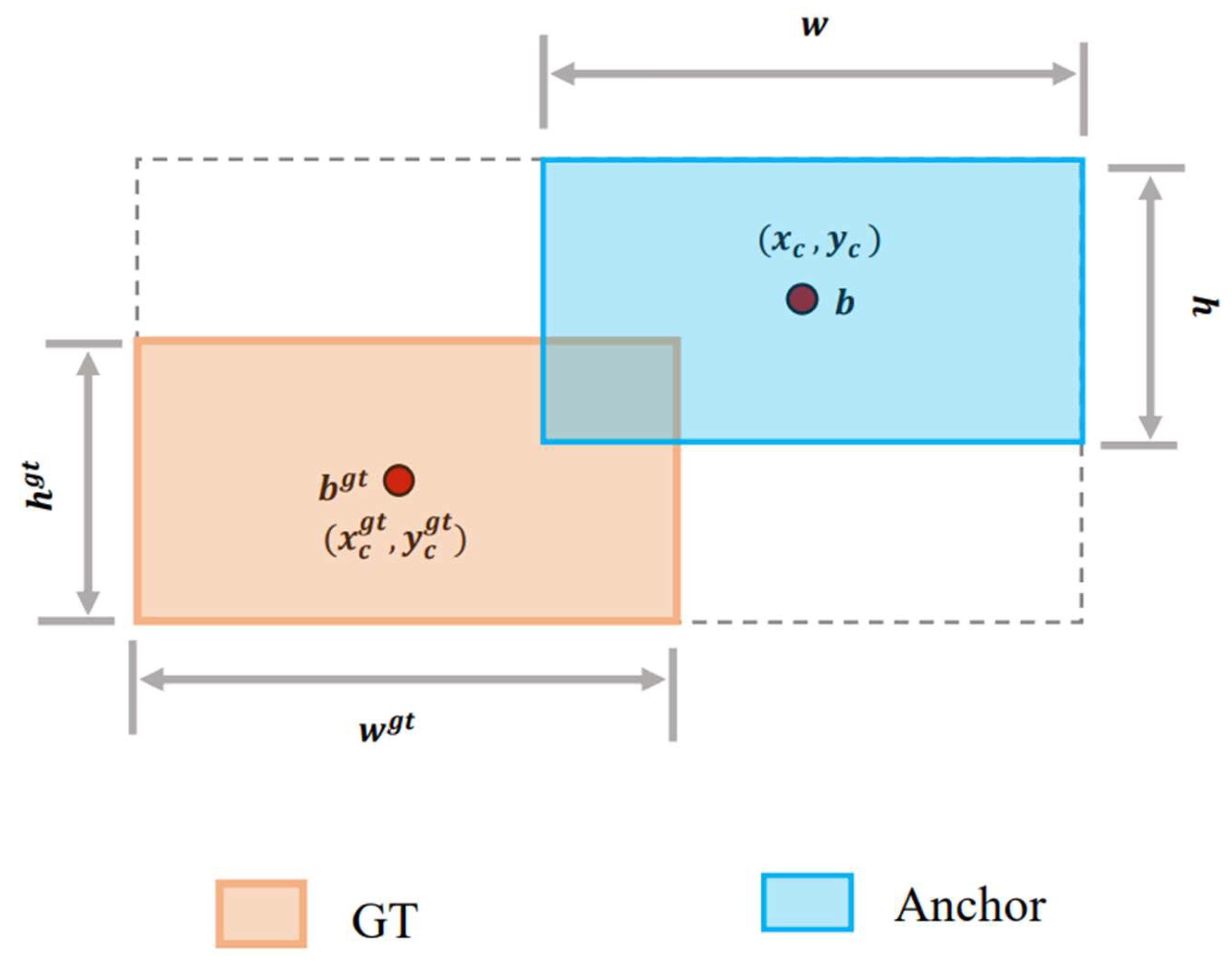
Formally, the Shape-Aware Wise IoU loss is given by

$$L_{\mathrm{Shape}\text{-}\mathrm{WiseIoU}}=L_{\mathrm{ShapeIoU}}\times \beta$$

(2)

$$L_{\mathrm{ShapeIoU}}=\left(1-IoU+{\mathrm{distance}}^{\mathrm{shape}}+0.5\times {\mathsf{\Omega }}^{\mathrm{shape}}\right)$$

(3)

The term ${\mathrm{distance}}^{\mathrm{shape}}$ penalizes the spatial displacement between the centers of the predicted box (Anchor) and the ground-truth box (GT), as shown in Figure 8. This displacement is weighted according to the aspect ratio of the GT box:

$${\mathrm{distance}}^{\mathrm{shape}}={\displaystyle \frac{{\left(x_c-x_c^{gt}\right)}^2}{c^2}}+{\displaystyle \frac{{\left(y_c-y_c^{gt}\right)}^2}{c^2}}$$

(4)

where

○

($x_c$,$y_c$): Center of the predicted (Anchor) box.

○

($x_c^{gt}$,$y_c^{gt}$): Center of the GT box.

○

$c^2$: Squared diagonal length of the smallest enclosing box (convex hull) covering both GT and Anchor. The values $cw$ and $ch$ correspond to the width and height of this enclosing box, respectively, and are computed as follows:

$$cw=\max \left(x_c+{\displaystyle \frac{w}{2}},x_c^{gt}+{\displaystyle \frac{w^{gt}}{2}}\right)-\min \left(x_c-{\displaystyle \frac{w}{2}},x_c^{gt}-{\displaystyle \frac{w^{gt}}{2}}\right)$$

(5)

$$ch=\max \left(y_c+{\displaystyle \frac{h}{2}},y_c^{gt}+{\displaystyle \frac{h^{gt}}{2}}\right)-\min \left(y_c-{\displaystyle \frac{h}{2}},y_c^{gt}-{\displaystyle \frac{h^{gt}}{2}}\right)$$

(6)

The squared diagonal of this convex box is then

$$c^2=c{w}^2+c{h}^2$$

(7)

${\mathsf{\Omega }}^{\mathrm{shape}}$ captures the difference in aspect ratios and sizes between GT and prediction, using an exponential decay to down-weight minor differences and emphasize significant ones:

$${\mathsf{\Omega }}^{\mathrm{shape}}=\sum _{t\in \{w,h\}}\left(1-e^{-{\mathsf{\omega }}_t^4}\right)$$

(8)

where

$${\mathsf{\omega }}_w={\displaystyle \frac{\left|w-w^{gt}\right|}{\max \left(h,h^{gt}\right)}},{\mathsf{\omega }}_h={\displaystyle \frac{\left|h-h^{gt}\right|}{\max \left(w,w^{gt}\right)}}$$

(9)

$\beta =\sqrt{{\displaystyle \frac{\mathrm{IoU}}{{\mathrm{IoU}}_{\mathrm{mean}}}}}$ acts as a monotonic scaling factor (adaptive focusing mechanism) that dynamically adjusts the contribution of each prediction to the total loss. This mechanism is inspired by Wise IoU’s philosophy of “confidence-aware regularization” and is crucial for maintaining stable optimization across diverse anomaly scales. Intuitively, $\beta$ increases when the predicted box quality (IoU) exceeds the average, encouraging the model to fine-tune and localize confident predictions even more precisely. Conversely, if the IoU is low (poor prediction or ambiguous object), β becomes smaller, reducing the penalty and preventing the model from being misled by difficult or noisy samples—such as small, broken cables that may only partially appear in the frame or exhibit low visual salience. Here, $\mathrm{Io}{\mathrm{U}}_{\mathrm{mean}}$ refers to the average IoU over all predictions in the current batch. It serves as a dynamic baseline that normalizes each individual IoU score, allowing the loss to adapt in real time to the difficulty level of each image or sample. This encourages the network to focus more on confident predictions when performance is high and down-weight uncertain predictions when performance is low.

Figure 8. Geometric interpretation of the Shape IoU formulation.

Figure 8. Geometric interpretation of the Shape IoU formulation.

These geometric relationships are visually illustrated in Figure 8 to aid interpretation and understanding.

Finally, following the same structure as A-YOLOM, the final loss function for PowerLine-MTYOLO combines all task-specific losses into a weighted sum, expressed as follows:

$$L_{\mathrm{total}}=L_{\det }+L_{\mathrm{seg}}$$

(10)

$$L_{\det }={\mathsf{\lambda }}_{\mathrm{cls}}{L}_{\mathrm{cls}}+{\mathsf{\lambda }}_{\mathrm{box}}{L}_{\mathrm{Shape}\text{-}\mathrm{WiseIoU}}+{\mathsf{\lambda }}_{\mathrm{dfl}}{L}_{\mathrm{DFL}}$$

(11)

$$L_{\mathrm{seg}}={\mathsf{\lambda }}_{\mathrm{TL}}{L}_{\mathrm{Tversky}}+{\mathsf{\lambda }}_{\mathrm{FL}}{L}_{\mathrm{Focal}}$$

(12)

where

• $L_{\mathrm{Shape}\text{-}\mathrm{WiseIoU}}$: Our proposed bounding-box loss incorporating Shape IoU and Wise IoU mechanisms.
• $L_{\mathrm{cls}}$: Binary Cross-Entropy (BCE) loss for classification.
• $L_{\mathrm{DFL}}$: Distribution Focal Loss (DFL) [31] for refining bounding-box predictions. DFL models the bounding-box regression task as a discrete distribution rather than a point estimate, enabling finer localization and better uncertainty modeling.
• $L_{\mathrm{seg}}$: Sum of Focal Loss and Tversky Loss for segmentation mask refinement. Focal Loss [32] addresses class imbalance by down-weighting easy examples and focusing learning on harder pixels, particularly useful in segmenting ambiguous or cluttered regions. Tversky Loss [33], an extension of Dice Loss, introduces asymmetric weighting of false positives and false negatives, making it especially effective for detecting small, thin structures like cables. Both are widely adopted in segmentation tasks.

The weighting factors ${\mathsf{\lambda }}_{\mathrm{cls}},{\mathsf{\lambda }}_{\mathrm{box}},{\mathsf{\lambda }}_{\mathrm{dfl}},{\mathsf{\lambda }}_{\mathrm{TL}},\mathrm{a}\mathrm{n}\mathrm{d}{\mathsf{\lambda }}_{\mathrm{FL}}$ were used to balance the contributions of classification, bounding-box regression, and segmentation losses during training. We adopted default values commonly recommended by the literature to ensure fair and reproducible comparisons with prior work. These weights were empirically calibrated to maintain stable training dynamics and prevent any task from dominating the optimization process. Specifically, we used ${\mathsf{\lambda }}_{\mathrm{cls}}=0.5$ for classification loss (BCE), ${\mathsf{\lambda }}_{\mathrm{box}}$ = 7.5 for bounding-box regression (Shape-Wise IoU), ${\lambda }_{\mathrm{dfl}}$ = 1.5 for Distribution Focal Loss (DFL), ${\lambda }_{\mathrm{TL}}$ = 8.0 for Tversky Loss, and ${\lambda }_{\mathrm{FL}}$ = 24.0 for Focal Loss.

These values were chosen to ensure a balanced contribution across tasks—detection and segmentation—even in the presence of class imbalance or small-scale objects, as is often the case in power line inspection.

2.3. Dataset Description

To train and evaluate our proposed model, we constructed the Merged Public Power Cable Dataset (MPCD) [34], a dedicated dataset targeting the inspection of high-voltage power lines via UAV imagery. This dataset aggregates images from five public sources available on the Roboflow Universe platform, one of the largest repositories of open-source computer vision datasets.

Table 1. Composition of the Merged Public Power Cable Dataset (MPCD), with image counts and corresponding data sources.

Dataset	Source	Number of Images
Daydantuacaothe1	[35]	1820
Daknonggd3	[36]	58
110_daydan_tua	[37]	100
Ddan_ct_tua	[38]	70
110_daydan_tua (tthpc)	[39]	116
Merged Public Power Cable Dataset (Ours)	[34]	1871

summarizes the composition of the MPCD in terms of image sources and counts.

All images were manually reviewed. Duplicates across datasets were removed to ensure quality and uniqueness. The resulting 1871 images were resized to 640 × 640 pixels to match YOLOv8’s default input resolution. Using the Roboflow annotation platform [40], we relabeled the dataset for two tasks: (1) pixel-wise segmentation of power line cables, and (2) object detection of broken cable strands. This detection class encompasses all instances of cable anomalies, including fractured strands and discontinuities. Each image was carefully verified to ensure the accuracy of both bounding boxes and masks.

Table 2. Final annotation statistics for detection and segmentation tasks in the MPCD.

Class	Number of Instances	Number of Images
Broken Cable	1906	-
Cable Segment	2501	-
Total	4407	1871

presents the final distribution of instances across the two tasks, demonstrating a relatively balanced number of broken cable annotations (1906) and segmented cable regions (2501), supporting multitask learning without introducing significant class imbalance.

The MPCD was intentionally constructed without additional manual augmentation. Instead, it benefits from YOLOv8’s built-in augmentation during training, including color jittering, flipping, rotation, and mosaic combinations. This approach ensures sufficient variability during learning while preserving the original image distributions.

Figure 9 provides qualitative examples from the MPCD, illustrating the diverse real-world conditions captured. The images span a wide range of UAV inspection scenarios, including rural, industrial, forested, and urban environments. Power lines appear with varying orientations, thicknesses, and lengths—sometimes intersecting or surrounded by cluttered backgrounds. This diversity reinforces the dataset’s realism and the challenges inherent in UAV-based inspection. To further illustrate the complexity of the detection and segmentation tasks, Figure 10 depicts the width–height distribution of annotated instances. Subfigure (a) corresponds to broken cable annotations, where the darker blue areas indicate high concentrations of objects with similar dimensions, typically exhibiting high aspect ratios. Subfigure (b) presents the distribution for cable segmentation masks, highlighting their dominant elongated form—long in width but thin in height. These patterns reveal the multi-scale and high-aspect-ratio nature of the task, which poses significant challenges to traditional detection and segmentation models. This observation directly motivates the design of PowerLine-MTYOLO, which includes shape-aware loss functions and architectural adaptations tailored for such scenarios.

From the final set of 1871 annotated images in the MPCD, we allocated 80% for training (1497 images) and 20% for validation (374 images). This standard split balances the need for robust model training with reliable performance evaluation. Given the moderate dataset size and the intricate nature of the task—particularly the detection of small, elongated, and visually subtle anomalies like broken cable strands—reserving a larger validation set ensures more statistically meaningful assessments of generalization. At the same time, the 80% training share provides sufficient data diversity for effective deep model learning.

The full MPCD is publicly available as an open-source resource [34].

2.4. Experimental Information

Environment Configuration: All experiments were conducted on Google Colab using an NVIDIA Tesla T4 GPU (15 GB VRAM) with CUDA 12.5 acceleration. The software environment was built on Python 3.11.11 with PyTorch 2.6.0+cu124 and Ultralytics YOLOv8.0.105, ensuring efficient training and evaluation.

This setup provided the necessary computational resources for training and validating the model while maintaining accessibility and scalability.

Models: To assess the effectiveness of PowerLine-MTYOLO, we conducted a targeted comparison against recent state-of-the-art (SOTA) YOLO-based models.

For multitask evaluation, we used the multitask SOTA model A-YOLOM (2024) as the baseline model, given its real-time joint detection and segmentation design. For detection benchmarking, we included the following recent lightweight models: YOLOv8n (2023), YOLOv9t (2023), YOLOv10n (2024), YOLOv11n (2024), YOLOv12n (2025), and Hyper-YOLOt (2024). Their corresponding segmentation variants—YOLOv8n-Seg to YOLOv12n-Seg—were used for evaluating the segmentation task.

All of these models belong to the nano configuration, which represents the smallest model size within the YOLO architecture spectrum. With parameter counts ranging between 2 M and 4 M, these configurations are optimized for edge deployment and low-latency applications, ensuring fair comparison across models in terms of complexity and resource consumption. This design choice aligns with our deployment objective, where UAV-based power line inspection must run on low-power edge devices.

Metrics: Following standard practices in the literature [41,42], we adopted task-specific evaluation metrics for both detection and segmentation. For anomaly (broken cable) detection, we reported the recall and mean average precision at IoU 0.5 (mAP@50), which are widely used to quantify localization accuracy and detection robustness.

For cable segmentation, we adopted Intersection-over-Union (IoU) and Line Accuracy (SubAcc) as evaluation metrics, following the setup introduced by A-YOLOM. IoU quantifies the spatial overlap between the predicted and ground-truth masks and remains a standard benchmark in segmentation tasks. However, due to the significant class imbalance—with background pixels vastly outnumbering those of the cable class—standard accuracy metrics can be misleading. To address this, we followed A-YOLOM by using Line Accuracy (SubAcc), which specifically evaluates performance on the minority class. Line Accuracy is computed as the average of sensitivity and specificity, providing a more equitable measure under imbalance:

$$\mathrm{SubAcc}={\displaystyle \frac{\mathrm{Sensitivity}+\mathrm{Specificity}}{2}}$$

(13)

$$\mathrm{with} \mathrm{Sensitivity}={\displaystyle \frac{TP}{TP+FN}},\mathrm{Specificity}={\displaystyle \frac{TN}{TN+FP}}$$

(14)

where $TP$, $FN$, $TN$, and $FP$ denote the true positives, false negatives, true negatives, and false positives, respectively. This formulation ensures that both false positives and false negatives are accounted for symmetrically, offering a more robust and fair evaluation of the model’s capacity to detect thin, low-contrast cable structures.

To assess computational efficiency, we report the inference speed in milliseconds per image. For practical real-time deployment, especially in UAV-based applications, inference must generally remain under 33.3 ms per frame to satisfy the 30 FPS threshold. We also report each model’s number of parameters and memory footprint (in megabytes, MB) to quantify the deployment cost and hardware compatibility.

Training Process and Evaluation Strategy: All models described earlier were trained using standardized hyperparameters provided by the Ultralytics framework to ensure fairness and reproducibility. Specifically, we employed the Stochastic Gradient Descent (SGD) optimizer with a fixed learning rate of 0.01, following common practice in YOLO-based training. No pretrained weights were used in any experiment; all models were trained from scratch, ensuring that none had prior exposure or bias toward the dataset. All detection metrics (precision, recall, mAP@50, mAP@50–95) were computed after applying Non-Maximum Suppression (NMS) with an IoU threshold of 0.7 to eliminate redundant overlapping predictions. Training was conducted for 150 epochs, with a batch size of 32 across all configurations. This epoch count was chosen based on empirical performance curves: as shown in Figure 11, loss functions—including box regression loss—begin to plateau after approximately 140 epochs. The validation mAP@50 also saturates during the same period, supporting the decision to terminate training early and prevent overfitting. Each training run required approximately 3 h on average using our computing environment. For evaluation, all models were assessed on the validation set. Evaluation was performed with a confidence threshold of 0.25 and an IoU threshold of 0.6, consistent with Ultralytics’ default inference parameters. This unified training and evaluation strategy ensured fair benchmarking across models.

3. Results

3.1. Our Model vs. A-YOLOM for Multitask Detection

To benchmark multitask performance, we compared our proposed PowerLine-MTYOLO model against the state-of-the-art multitask baseline A-YOLOM-nano. As shown in

Table 3. Comparison of PowerLine-MTYOLO and A-YOLOM-nano in terms of multitask performance, efficiency, and model size.

Models	mAP@50	Recall	IoU	SubAcc	Speed (in ms)	Parameters (in Millions)	Model Size (MB)
AYOLO-M-nano	0.693	0.872	0.752	0.915	3.4	3.19 M	6.9 MB
Our Model	0.767 (+10.68%)	0.877	0.767	0.932	3.5	2.96 M	6.2 MB (−10.14% lighter)

Note: The bold values represent the best results for their respective metrics.

, our model achieves a +10.68% relative improvement in mAP@50 (0.767 vs. 0.693), indicating significantly better localization accuracy in detecting broken cable strands. SubAcc also increases from 0.915 to 0.932, highlighting stronger classification confidence for fine-grained segmentation prediction. Despite this gain in accuracy, our model remains lightweight, with a 10.14% smaller model size (6.2 MB vs. 6.9 MB) and fewer parameters (2.96 M vs. 3.19 M), making it more suitable for edge deployment. The inference time remains comparable, at 3.5 ms per instance, ensuring that real-time capability is preserved. These results validate the effectiveness of our architectural and loss design enhancements, achieving both higher accuracy and better efficiency than A-YOLOM under the same resource constraints.

These quantitative improvements are supported by qualitative results, as shown in Figure 12. The first two rows illustrate cases involving broken cable anomalies. While A-YOLOM fails to detect these anomalies entirely, our model successfully localizes them with reasonable confidence levels of 0.80, 0.53, and 0.25, respectively. These results confirm the enhanced anomaly sensitivity of our approach, even in challenging cases where the visual contrast between cable and background is low. For the segmentation task in these examples, both models achieve generally consistent cable masks, indicating comparable performance in the presence of broken strands.

Furthermore, in rows 3 and 4—where no anomalies are present and the focus is solely on cable segmentation—PowerLine-MTYOLO more accurately follows the geometry of the cables, particularly in regions where the structures are extremely thin or partially occluded. As highlighted by the red arrows, A-YOLOM tends to produce more fragmented or incomplete masks under these conditions, whereas our model better preserves structural continuity.

Statistical Evaluation of Performance Differences:

An important question arises when comparing model performance: “Are the observed gains of PowerLine-MTYOLO over A-YOLOM statistically significant, or could they be due to chance?” While it is standard practice to report single-run results, such evaluations may overlook variability stemming from random initialization, data shuffling, or training dynamics. This concern is especially relevant in our case, given the relatively small size of the test set, which increases the risk of overestimating performance from a single experiment. To mitigate this risk and ensure that the improvements of our model are robust rather than incidental, we followed a well-established experimental protocol: training both models across multiple random seeds and applying statistical significance testing, as recommended in prior works [43,44].

Table 4. Multi-seed evaluation of PowerLine-MTYOLO vs. A-YOLOM across key metrics.

Seed	Model	mAP@50	IoU	SubAcc	Recall
0	Ours	0.767	0.767	0.932	0.877
0	A-YOLOM	0.693	0.752	0.915	0.872
42	Ours	0.756	0.769	0.926	0.864
42	A-YOLOM	0.722	0.757	0.916	0.869
99	Ours	0.759	0.773	0.933	0.890
99	A-YOLOM	0.743	0.768	0.923	0.877
2025	Ours	0.738	0.779	0.932	0.869
2025	A-YOLOM	0.744	0.767	0.924	0.880

reports results across four seeds (0, 42, 99, and 2025), comparing PowerLine-MTYOLO and A-YOLOM on four key metrics: mAP@50, IoU, SubAcc, and recall. Our model outperforms the baseline in mAP@50 and SubAcc for every seed, with especially notable gains at seed 0 (+10.68% in mAP@50, +0.017 in SubAcc). The IoU score also consistently favors PowerLine-MTYOLO, indicating more precise boundary estimation in segmentation masks. Recall shows more variability but remains competitive.

To assess statistical significance, we applied a paired t-test on the four repeated measures. The results show that the differences in IoU (p = 0.0139) and SubAcc (p = 0.0107) are statistically significant (p < 0.05), confirming consistent improvements in segmentation accuracy. However, mAP@50 (p = 0.13) and recall (p = 0.93), though consistently higher in our model, do not reach statistical significance, likely due to the small sample size (N = 4).

These results confirm that the performance improvements of our multitask model are not only consistent across multiple random seeds but also statistically significant for key metrics such as IoU and SubAcc. While we acknowledge that a larger-scale evaluation (e.g., using 20 or more seeds) would provide stronger statistical power, our experiments were limited to four seeds due to computational constraints. Nonetheless, the consistent superiority of our model across runs—combined with statistically significant gains in segmentation accuracy—reinforces the validity and reproducibility of the improvements brought by the PowerLine-MTYOLO architecture over the A-YOLOM baseline.

3.2. Detection Performance Comparison

To assess detection capabilities, we compared PowerLine-MTYOLO against several recent real-time object detectors from the YOLO family discussed earlier. As summarized in

Table 5. Comparison of detection performance between PowerLine-MTYOLO and recent YOLO-based nano models on the MPCD.

Models	mAP@50	Recall	Speed (in ms)	Parameters (in Millions)	Model Size (MB)
YOLOv8n	0.732	0.630	2.897	3.01 M	6.3 MB
YOLOv9t	0.732	0.618	4.154	2.00 M	4.6 MB
YOLOv10n	0.649	0.600	3.796	2.70 M	5.8 MB
YOLOv11n	0.734	0.624	3.179	2.59 M	5.5 MB
YOLOv12n	0.690	0.606	5.018	2.56 M	5.5 MB
Hyper-YOLOt	0.732	0.650	4.007	3.01 M	6.3 MB
Our Model	0.767	0.877	3.5	2.96 M	6.2 MB

Note: The bold values represent the best results for their respective metrics.

, our model outperformed all compared models in terms of mAP@50, achieving 0.767, the highest among all nano-scale architectures. The closest competitors—YOLOv8n, YOLOv9t, YOLOv11n, and Hyper-YOLOt—plateau between 0.732 and 0.734, yielding a relative improvement of +4.5% for our model.

Importantly, recall sees a substantial boost, reaching 0.877 in our model compared to 0.650 for Hyper-YOLOt and 0.630 for YOLOv8n, representing a relative improvement of +34.9% and +39.2%, respectively. This significant gain highlights enhanced detection coverage, particularly for challenging and small-scale broken cable instances. Despite these improvements in accuracy, PowerLine-MTYOLO maintains a competitive inference time of 3.5 ms, placing it within the same real-time category as other lightweight detectors.

In terms of efficiency, our model preserves a compact architecture with 2.96 million parameters and a 6.2 MB memory footprint, demonstrating that performance improvements were achieved without compromising computational constraints. This balance between detection accuracy and model efficiency reinforces the suitability of PowerLine-MTYOLO for UAV-based power line inspection tasks, where both real-time performance and lightweight deployment are critical.

Also, Figure 13 offers a visual comparison of detection performance across models in challenging scenarios. In the first column, the broken cable anomaly is subtle—only a thin, slightly displaced strand is visible against a clean sky. Our model successfully detects the anomaly, with a confidence of 0.35, while other models either miss the defect entirely or predict with lower confidence (YOLOv11n: 0.27, YOLOv8n: 0.31, Hyper-YOLOt: 0.27). The second column depicts a cable defect located near a metallic pylon, where the cable visually blends with the background due to color similarity. Despite this camouflage, our model correctly identifies the anomaly, with 0.39 confidence, outperforming alternatives such as YOLOv9t (0.34) and Hyper-YOLOt (0.29), which either misclassify the structure or exhibit lower reliability. In the third column, the cable anomaly is small and partially obscured by a dense forest background. Our model demonstrates precise localization, detecting the defect with 0.28 confidence. Although other models sometimes identify this region, their predictions are poorly localized, often covering large portions of the cable rather than isolating the actual damaged area. In the fourth column, the anomaly is positioned in the upper-left region of the frame and partially merges with a deteriorated wall exhibiting cracks that resemble cable defects. This spatial marginality and background ambiguity pose serious challenges for detection. While YOLOv8n, YOLOv9t, and YOLOv12n do offer low-confidence predictions (ranging from 0.27 to 0.35), our model not only detects the defect but does so with a significantly higher confidence of 0.67, highlighting its enhanced ability to reason about weak and off-center anomalies under visually misleading contexts.

3.3. Segmentation Performance Comparison

Table 6. Comparison of segmentation performance between PowerLine-MTYOLO and recent YOLO-based nano models on the MPCD.

Models	IoU	SubAcc	Speed (in ms)	Parameters (in Millions)	Model Size (MB)
YOLOv8n-Seg	0.727	0.845	3.719	3.26 M	6.8 MB
YOLOv9t-Seg	0.728	0.842	6.976	3.12 M	6.9 MB
YOLOv10n-Seg	0.731	0.845	4.092	2.84 M	6.0 MB
YOLOv11n-Seg	0.749	0.846	3.757	2.84 M	6.0 MB
YOLOv12n-Seg	0.733	0.845	4.527	2.8 M	6.1 MB
Our Model	0.767	0.932	3.5	2.96 M	6.2 MB

Note: The bold values represent the best results for their respective metrics.

presents a comparison of segmentation performance between PowerLine-MTYOLO and recent YOLO-based models designed for segmentation prediction tasks. Our model achieves the highest Intersection-over-Union (IoU) score of 0.767, surpassing the best competitor, YOLOv11n-Seg, which reaches 0.749, yielding a +2.4% improvement in segmentation accuracy. Compared to YOLOv8n-Seg, the improvement rises to +5.5%, highlighting the robustness of our model in capturing elongated and thin structures typical of power line cables. The Line Accuracy (SubAcc), which evaluates fine-grained pixel-wise correctness, is significantly improved, reaching 0.932 for PowerLine-MTYOLO—+10.2% higher than YOLOv11n-Seg (0.846) and +10.3% higher than YOLOv8n-Seg (0.845). This indicates the strong ability of our architecture and segmentation head to preserve cable continuity and refine structural boundaries. Importantly, our model maintains this superior segmentation performance without compromising efficiency. It operates at 3.5 ms per image, faster than YOLOv9t-Seg (6.976 ms) and slightly faster than YOLOv11n-Seg (3.757 ms), making it suitable for real-time UAV-based inspection. The model remains lightweight, with 2.96 M parameters and a size of 6.2 MB, ensuring deployment feasibility on edge devices.

To further illustrate the segmentation capabilities of our proposed model, Figure 14 presents qualitative results on representative images from the validation set. Each column highlights a different challenge scenario for power line segmentation. In the first column, the images contain relatively few cables, but the cables themselves are very thin and fade into the cloudy sky background. While most models struggle with pixel-level precision and fail to segment all visible cables, our model achieves complete segmentation of each cable, accurately following their structure without mistakenly including background pixels. This result underscores the model’s enhanced ability to preserve thin, linear structures. The second column presents a dense and visually complex scenario, where multiple power lines intersect and overlap against a gray, low-contrast sky. Among all of the models, only our method and YOLOv9-Seg manage to produce acceptable results. Although some cables remain partially undetected, this highlights that there is still room for improvement under such dense and visually complex conditions. In the third column, the target cable is surrounded by vegetation and ambiguous objects, including a thin wooden stick with similar appearance to the cable. Several models mistakenly segment this distractor. In contrast, our model and YOLOv9-Seg successfully isolate the correct cable with minimal false positives, highlighting stronger semantic understanding and robustness against background interference.

3.4. Explanation and Analysis

The superior performance of PowerLine-MTYOLO can be attributed to the synergistic effect of its architectural modifications and loss function design, each carefully tailored to the visual and structural challenges of UAV-based power line inspection. First, the integration of the Shared Dilation Pyramid Module (SDPM) enhances multi-scale feature extraction, enabling the model to better capture both small, localized anomalies and long-range contextual cues. The use of depthwise separable convolutions with varying dilation rates allows the SDPM to expand the receptive field without sacrificing spatial resolution—an essential trait for detecting subtle cable defects and maintaining the continuity of thin structures like power lines. This multi-scale awareness explains the model’s superior generalization to both close-up and wide-view cable scenarios, as evidenced in Figure 13 and Figure 14. In particular, the fourth column in Figure 14 offers an illustrative case where, although the model fails to segment the actual cable due to strong visual interference with the pylon structure, it produces structured false positives aligned with the metallic bars, suggesting that the model assigns high-level semantic relevance to visually similar linear features. This exploratory behavior may reflect the influence of the SDPM: by leveraging multiple dilation rates, it enables broader contextual awareness, potentially enhancing the model’s theoretical capacity to generalize across ambiguous or unseen patterns. Second, the Edge-Enhanced Refinement (EFR) segmentation head plays a critical role in improving pixel-wise prediction quality. By applying a learnable edge enhancement mechanism at the entrance of the decoding path, the model becomes more sensitive to cable boundaries, even when they blend into complex backgrounds. This attention to boundary fidelity reduces segmentation fragmentation and background misclassification, a common failure mode in cable segmentation tasks. As illustrated in Figure 14, this leads to higher SubAcc and IoU scores, since the predicted masks align more tightly with the true cable structures, avoiding both excessive blurring and erroneous inclusion of background pixels (i.e., the segmentation produced by other models appears blurrier than that of our method). Third, the inclusion of the Hierarchical Attention Detection (HAD) head also contributes to improved detection by refining spatial and channel-level representations through attention-guided bottlenecks. This enables the model to prioritize informative features—particularly important when distinguishing small, defect-like anomalies from normal cable segments or visually confusing background pixels (as illustrated in Figure 13, where the cable blends into the pylon background). Finally, the adoption of the Shape-Aware Wise IoU loss encourages the model to learn bounding-box predictions that are not only spatially aligned but also shape-consistent. This is particularly important for detecting fine-grained structural anomalies that affect only a small section of long cables. The shape-aware penalty term guides the model to produce tighter, more localized bounding boxes, avoiding the overextended or imprecise detections commonly seen in baseline models. This behavior, observed in Figure 13 (second and third columns), leads to improved mAP@50 while enhancing interpretability in defect localization. Collectively, these innovations explain the observed gains in both detection and segmentation tasks under challenging real-world conditions. The architectural design and loss functions complement each other in promoting structural consistency, shape sensitivity, and edge precision—key factors in improving UAV-based power line inspection performance.

Nevertheless, despite these improvements, certain failure modes persist. As depicted in the fifth column of Figure 14, our model failed to detect an additional cable (which is in a normal state) that is clearly visible in the upper part of the image—a relatively straightforward case with minimal background interference. Interestingly, other models such as YOLOv9 and YOLOv8 managed to detect this cable. One plausible explanation lies in the multitask training dynamics of our model: The shared forward and backward pass between segmentation and anomaly detection may bias the model towards structures that are likely to contain anomalies. This implicit prioritization could lead to occasional under-segmentation of visually “normal” cables. While this behavior reflects the model’s joint-task learning focus, it also reveals a potential limitation. A promising mitigation strategy would involve enriching the training dataset with more cable instances that are anomaly-free, ensuring balanced learning and reinforcing the model’s ability to generalize across both defective and intact cable segments. Furthermore, a related limitation can be observed in the fifth column of Figure 13, where all models fail to detect the anomaly except for YOLOv11n, which achieves a confidence of 0.34. The challenge arises from the visual camouflage created by a dense vegetation background, which makes the anomaly difficult to distinguish. YOLOv11n’s success in this case may be attributed to the inclusion of spatial attention modules (such as the C2PSA block), which enhance its ability to focus on subtle, spatially relevant features. This observation suggests that augmenting our own architecture with additional attention mechanisms—potentially in the backbone rather than solely in the head—could improve performance in such scenarios. However, this comes with a trade-off in computational cost, and further exploration would be required to evaluate its feasibility.

3.5. Generalization to Unseen UAV Data

To assess the generalization capability of our model beyond the training distribution, we conducted a comparative evaluation against A-YOLOM, as it also addresses the same multitask problem of simultaneous cable segmentation and anomaly detection. This choice ensured a fair and meaningful benchmark, as both models were trained on the same dataset (MPCD) and shared comparable UAV-based deployment objectives.

To perform this evaluation under real-world conditions, we selected a video recorded in 2022 during a live inspection session in Casablanca, Morocco. The data were collected using a GoPro Hero 7 camera mounted on a drone equipped with a Pixhawk autopilot system. The inspection site was a training facility managed by the ONEE (National Office of Electricity and Drinking Water, Morocco), where various known defects are intentionally present to support the training of human inspectors. This environment introduces diverse and realistic challenges, including varying vegetation density and subtle defects, as shown in Figure 15. We chose this dataset because, to the best of our knowledge, the MPCD remains the only publicly available dataset combining both power cable segmentation and broken strand detection in a unified multitask setting. Therefore, to assess cross-domain robustness in practical settings, we conducted preliminary tests on this independent dataset acquired in collaboration with the ONEE.

The selected test set comprised 121 manually annotated frames, including 39 images containing visible cable anomalies (e.g., broken strands) and 82 images depicting normal cable configurations.

We used the pretrained versions of both models—trained solely on the MPCD—to ensure a fair and reproducible evaluation. No fine-tuning or domain adaptation was performed, thereby testing each model’s robustness in a previously unseen environment.

Quantitative results are reported in

Table 7. Quantitative results on the unseen UAV footage from Casablanca. Both models were trained on the MPCD and evaluated directly on the new test set without fine-tuning.

Model	Recall	mAP@50	IoU	SubAcc
A-YOLOM	0.589	0.491	0.642	0.836
Ours	0.726	0.471	0.656	0.860

Note: The bold values represent the best results for their respective metrics.

, using a fixed evaluation threshold (IoU = 0.6, confidence = 0.25). While both models exhibit overall performance degradation compared to their original test results (a known effect under domain shift), PowerLine-MTYOLO demonstrates stronger generalization over A-YOLOM.

Despite a slight drop in mAP@50 compared to A-YOLOM (0.471 vs. 0.491), our model significantly outperformed it in recall (+0.137), IoU (+0.014), and sub-pixel accuracy (+0.024). These improvements confirm that PowerLine-MTYOLO is better equipped to handle complex multitask inspection scenarios under domain shift.

Qualitatively, Figure 16 confirms that PowerLine-MTYOLO provides more continuous and reliable segmentation across scenes. It successfully detects anomalies and maintains cable continuity, even in visually challenging settings. For instance, in the first column, the model accurately segments the upper and lower cables and detects a broken strand missed by A-YOLOM. In the second example, it also provides better structural consistency.

In conclusion, while this test does not constitute a full statistical benchmark, it highlights the promising generalization performance of our multitask architecture for UAV-based infrastructure inspection in unseen real-world scenarios.

3.6. Ablation Study 1

Furthermore, to understand the individual and combined contributions of the proposed modules in PowerLine-MTYOLO, we conducted a systematic ablation study, as presented in

Table 8. Ablation study on the individual and combined impact of the SDPM, HAD-Head, EFR-Seg, and Shape-Aware Wise IoU on the detection and segmentation performance of PowerLine-MTYOLO.

Ablation N°	SDPM	HAD-Head	EFR-Seg	Shape-Aware Wise IoU	mAP@50	Recall	IoU	SubAcc	Speed (in ms)	Parameters (in Millions)	Model Size (MB)
1 (Baseline)					0.693	0.872	0.752	0.915	3.4	3.19 M	6.9 MB
2	✓				0.726	0.88	0.76	0.922	3.5	3.43 M	7 MB
3	✓	✓			0.722	0.883	0.764	0.924	3.6	2.96 M	6.3 MB
4	✓		✓		0.723	0.864	0.758	0.919	3.5	3.44 M	7 MB
5	✓	✓	✓		0.748	0.89	0.754	0.911	3.5	2.96 M	6.2 MB
6		✓			0.717	0.903	0.752	0.923	3.5	2.84 M	6.2 MB
7		✓	✓		0.738	0.919	0.752	0.919	3.5	2.84 M	6.2 MB
8		✓		✓	0.738	0.898	0.77	0.922	3.4	2.84 M	6.2 MB
9		✓	✓	✓	0.747	0.906	0.773	0.924	3.5	2.84 M	6.2 MB
10			✓		0.721	0.885	0.767	0.926	3.5	3.31 M	7 MB
11			✓	✓	0.727	0.885	0.769	0.924	3.5	3.32 M	7 MB
12				✓	0.719	0.88	0.773	0.934	3.4	3.19 M	6.9 MB
13	✓			✓	0.745	0.854	0.773	0.928	3.6	3.4 M	7 MB
14	✓	✓		✓	0.75	0.849	0.76	0.922	3.5	2.96 M	6.3 MB
15	✓		✓	✓	0.721	0.854	0.773	0.925	3.5	3.4 M	7 MB
16 (Full_Our)	✓	✓	✓	✓	0.767	0.877	0.767	0.932	3.5	2.96 M	6.2 MB

Note: The bold values represent the best results for their respective metrics. The symbol ✓ indicates that the corresponding module is included in the ablation configuration.

.

Starting from the A-YOLOM-nano baseline (Ablation 1), we incrementally activated each component—SDPM, HAD-Head, EFR-Seg, and the Shape-Aware Wise IoU loss—and observed their impact on performance across detection and segmentation tasks. Table 8 summarizes the results. When added individually, each component improves key metrics, validating their complementary design goals. The Shared Dilation Pyramid Module (SDPM) alone (Ablation 2) yields a +4.8% increase in mAP@50 (0.726 vs. 0.693), confirming its effectiveness in capturing multi-scale features, especially for detecting small anomalies. Importantly, this gain is achieved with only a minimal increase in inference latency (3.5 ms vs. 3.4 ms) and a modest rise in model size (7.0 MB vs. 6.9 MB). This favorable trade-off is due to the shared-weights strategy adopted within the SDPM, which limits parameter growth (3.43 M vs. 3.19 M) despite using parallel dilated branches. The Hierarchical Attention Detection (HAD) head (Ablation 6) significantly improves recall (0.903 vs. 0.872, +3.55%) and mAP@50 (0.717 vs. 0.693, +3.46%). Despite these gains, its parameter count is the lowest among all evaluated modules (2.84 M), with no increase in inference time (3.5 ms) and a compact model size of only 6.2 MB. This computational efficiency stems from two architectural optimizations: First, the HAD head integrates shared-weight convolutions, forming a bottleneck structure that minimizes redundancy across scales. Second, unlike the original A-YOLOM head, which uses two separate branches—one for classification and one for box regression—we fuse both branches into a shared processing path, which significantly reduces the duplication of computation and parameters. Only after the shared hierarchical backbone do we apply small, task-specific projection heads for classification and box prediction.

This design maintains the functional separation of the two tasks while achieving better parameter efficiency and feature reuse, making the HAD head a lightweight yet effective enhancement over the original detection head. The Edge-Enhanced Refinement (EFR) segmentation head (Ablation 10) notably improves SubAcc (0.926 vs. 0.915, +1.20%) and IoU (0.767 vs. 0.752, +1.99%), as it reinforces the structural continuity of thin cables via learnable edge refinement. Its inference speed remains modest (3.31 M vs. 3.19 M parameters, 7.0 MB vs. 6.9 MB size, 3.4 ms vs. 3.5 ms latency), as the module uses only average pooling and a pair of lightweight 1 × 1 convolutions, which are known to be highly efficient on modern accelerators. This makes EFR-Seg a particularly attractive addition for improving segmentation without compromising deployability. The integration of Shape-Aware Wise IoU loss (Ablation 12) produces a clear boost in IoU (0.773 vs. 0.752, +2.79%) and mAP@50 (0.719 vs. 0.693, +3.75%), highlighting its role in improving bounding-box precision for small and elongated defects. Interestingly, this module slightly reduces recall, as the loss formulation encourages more spatially precise predictions and penalizes overly large boxes, resulting in better localization but fewer loose detections. This is the trade-off between quantity (recall) and quality (precision/IoU). As a loss function, Shape-Aware Wise IoU does not impact inference latency or parameter count, since it is only applied during training.

Combined configurations reveal further insights. For example, the combination of HAD + EFR + Shape-Aware Wise IoU (Ablation 9) achieves a strong, balanced performance (mAP@50 = 0.747, IoU = 0.773, SubAcc = 0.924) while remaining lightweight (6.2 MB).

Our full model (Ablation 16), which integrates all four components, achieves the best overall performance, with mAP@50 = 0.767, recall = 0.877, IoU = 0.767, and SubAcc = 0.932, while reducing the model size by 10.14% compared to the baseline.

These findings validate the design of PowerLine-MTYOLO: each module addresses a specific challenge—whether multi-scale perception, structural continuity, or localization precision—and their integration results in significant gains without compromising efficiency.

3.7. Ablation Study 2

To further validate the design rationale of our Edge Enhancer module in the segmentation head, we conducted an additional ablation study comparing it against several alternative edge enhancement strategies. All experiments were conducted within the same segmentation branch of PowerLine-MTYOLO and trained using identical setups, ensuring fair and reproducible comparisons. The goal of this evaluation was not to establish a comprehensive benchmark—which falls beyond the scope of this study—but, rather, to support the positioning of our design among existing approaches.

Table 9. Ablation study comparing different edge enhancement strategies integrated within the segmentation branch of PowerLine-MTYOLO.

#	Edge Enhancement Strategy	Type	mAP@50	Recall	IoU	SubAcc	Speed (ms)	Parameters (M)
1	Sobel Filter [23]	Non-Learnable (Gradient)	0.721	0.885	0.767	0.926	3.5	2.96
2	Laplacian Filter (Marr–Hildreth) [45]	Non-Learnable (Second-Order)	0.719	0.880	0.773	0.934	3.5	2.96
3	HED-Style CNN Module [25]	Learnable (Multi-Scale CNN)	0.755	0.879	0.771	0.926	8.5	2.98
4	PiDiNet-Based Enhancer [26]	Learnable (Lightweight CNN)	0.745	0.854	0.773	0.928	3.6	3.40
5	AERNet-Based Attention Enhancer [27]	Learnable (Attention-Based)	0.750	0.849	0.760	0.922	3.5	2.96
6	Edge Enhancer Module (Ours)	Learnable (Pooling + Conv)	0.767	0.877	0.767	0.932	3.5	2.96

Note: The bold values represent the best results for their respective metrics.

presents the performance comparison between our Edge Enhancer and five alternative modules, spanning both non-learnable and learnable paradigms. In this analysis, we emphasize IoU and SubAcc as the primary evaluation metrics for the segmentation task, as they directly reflect the ability to capture thin, continuous structures like power line cables. However, given that all of the modules are trained end-to-end with a shared loss, we also report mAP@50 and recall to account for any upstream influence on detection performance due to shared gradient updates.

Non-learnable operators—namely the Sobel and Laplacian filters—demonstrate surprisingly competitive performance in terms of segmentation. The Sobel filter yields a solid IoU of 0.767 and SubAcc of 0.926, validating its ability to extract coarse edge transitions even without adaptation. The Laplacian filter [45], which captures second-order intensity changes, improves further, with an IoU of 0.773 and SubAcc of 0.934, suggesting superior boundary sensitivity. However, both methods slightly degrade mAP@50 and recall, indicating that their fixed nature may introduce artifacts or misaligned signals that confuse the detection branch during joint training. This highlights a key limitation: while effective for segmentation, non-learnable enhancements may conflict with detection-level optimization due to their rigid, non-adaptive nature.

In contrast, learnable edge modules offer more balanced trade-offs across tasks. The HED-style CNN, which leverages deep multi-scale feature fusion, achieves strong segmentation metrics (IoU = 0.771, SubAcc = 0.926) while also preserving relatively high mAP@50 (0.755). However, this comes at a computational cost (8.5 ms), which may not be suitable for edge-deployed UAV applications. The PiDiNet-based module, designed for efficient edge detection via pixel-difference operations and compact dilated convolutions, reaches the same IoU of 0.773 and a SubAcc of 0.928 with a lower latency and parameter count, proving particularly attractive for real-time scenarios. The AERNet-inspired attention module offers a more spatially focused enhancement but exhibits slightly reduced IoU (0.760) and SubAcc (0.922), possibly due to over-attending to dominant contours and underrepresenting finer edges. Notably, all learnable modules maintain high mAP@50 and recall, demonstrating their ability to harmonize with the detection head during training. This consistency stems from their adaptive nature, allowing them to selectively emphasize meaningful edge features while avoiding the rigid impositions of handcrafted operators. As such, they achieve strong segmentation performance without penalizing the detection metrics too much.

Our Edge Enhancer module achieves the highest SubAcc (0.932) among all tested variants and a competitive IoU of 0.767. More importantly, it maintains balanced performance across detection (mAP@50 = 0.767, recall = 0.877), segmentation, and efficiency (2.96 M parameters, 3.5 ms). Its residual structure—based on average pooling subtraction followed by lightweight convolution—preserves the semantic fidelity of the base features while enhancing edge-localized signals in a non-destructive manner. This architectural balance allows the model to improve segmentation performance without negatively impacting detection learning during joint training.

4. Discussion

Compared to A-YOLOM, our model achieved a +10.68% improvement in mAP@50 (0.767 vs. 0.693) and a +2.0% boost in IoU (0.767 vs. 0.752), while also being 10.14% lighter (6.2 MB vs. 6.9 MB). Importantly, these improvements were achieved without increasing the inference time or model parameters, highlighting the effectiveness of targeted, domain-aware architectural enhancements. The real-time processing capability of 3.5 ms per frame confirms its operational readiness for deployment in UAV systems.

While the evaluation was conducted on server-grade hardware (Tesla T4 GPU), it is worth noting that YOLOv8—our underlying framework—has demonstrated over 100 FPS on embedded platforms like the Jetson Orin Nano when TensorRT-optimized [46,47,48]. Since our model is lighter than A-YOLOM, similar or better efficiency is expected, making it well suited for real-time onboard inference in edge UAV systems.

In terms of generalization, the improvements proposed in PowerLine-MTYOLO—particularly those targeting shape awareness and structural continuity—may extend to other industrial monitoring tasks involving elongated or fine-grained features, such as crack detection in pavements, pipeline inspection, or wiring trace analysis in electrical grids. Future validation in these application areas will be necessary to confirm this broader potential.

Moreover, PowerLine-MTYOLO opens a new direction for unified multitask frameworks in aerial infrastructure inspection. Instead of relying on sequential pipelines—where segmentation and component-specific anomaly detection are handled in two disjoint phases—our approach suggests a scalable architecture where both tasks can be integrated within a single-stage model. Beyond broken strands and cables, the same design principles can be extended to simultaneously segment other components (e.g., insulators) and detect multiple types of anomalies (cracks, corrosion, loose fittings). Thanks to its modular structure, our model supports flexible head and neck configurations, making it suitable for multi-class, multi-region segmentation and detection. This opens opportunities for inspection pipelines capable of addressing a broad range of operational requirements.

Furthermore, to the best of our knowledge, this work represents the first multitask architecture specifically tailored for the simultaneous detection of anomalies and segmentation of power cables in UAV imagery. Additionally, the Merged Public Power Cable Dataset (MPCD), introduced in this study, is the first openly curated dataset to jointly support both cable segmentation and defect detection, making it a valuable resource for advancing research in UAV-based power line inspection.

Despite these contributions, this study has a few limitations. While we designed the Merged Public Power Cable Dataset (MPCD) to capture a wide range of real-world scenarios, testing remained confined to this dataset. Although it covers diverse visual conditions (e.g., forests, urban scenes, metal towers, complex backgrounds), cross-dataset generalization remains to be assessed. For detection- or segmentation-only tasks, additional datasets such as the TTPLA dataset [49] or PLD-UAV dataset [5] may serve as important future benchmarks. However, while we did conduct preliminary tests using UAV footage collected during a previous inspection in Casablanca, Morocco (video available via our GitHub repository [34]), this represents only a small real-world validation scenario. The model performed quite strongly despite never being exposed to these images, suggesting good generalization, but comprehensive field testing remains essential.

Additionally, future extensions of the MPCD may include a broader range of cable-related anomalies, such as foreign objects, fallen branches, or external mechanical interference. This would enable the dataset to more fully represent the spectrum of real-world faults and further support the development of generalized anomaly detection models. Moreover, we plan to introduce challenging weather conditions—such as fog, rain, and low-light visibility—to simulate adverse inspection scenarios. These additions will be critical for assessing the robustness of detection and segmentation models in realistic field environments, and they will represent an important step toward building more weather-resilient inspection pipelines.

Also, while our current Edge Enhancer offers a lightweight and effective solution, we acknowledge that more advanced designs could further improve the segmentation of very fine structures such as thin cables. In future work, enhancement mechanisms may move beyond average pooling toward more adaptive or task-specific attention-based strategies.

Looking ahead, a promising direction involves developing a fully autonomous UAV system capable of simultaneous navigation and inspection using cable segmentation as a visual guide. Prior works, such as [50,51], have proposed leveraging segmentation maps of power lines to inform drone trajectory planning, altitude correction, or real-time obstacle avoidance. Extending PowerLine-MTYOLO into such closed-loop systems represents a natural evolution, allowing for real-time anomaly detection and autonomous path planning in a unified framework.

5. Conclusions

This study presented PowerLine-MTYOLO, a lightweight multitask model optimized for UAV-based inspection of high-voltage power cables. By integrating four specialized novel architectural modules—SDPM, HAD, EFR, and the Shape-Aware Wise IoU loss—this model effectively addresses the challenges of detecting small-scale anomalies and segmenting thin, elongated structures under diverse real-world conditions.

To enable rigorous evaluation, we also introduced the Merged Public Power Cable Dataset (MPCD), a carefully curated dataset constructed from multiple open-access sources and manually annotated to support both detection and segmentation tasks. The MPCD captures a wide range of realistic inspection scenarios, including complex backgrounds, varied cable geometries, and challenging visual conditions.

Extensive experiments on the MPCD demonstrated notable gains in both detection and segmentation performance, achieving up to +10.68% mAP@50 and +1.7% IoU compared to the strong A-YOLOM baseline, while remaining computationally efficient and even lighter in model size. In addition, PowerLine-MTYOLO consistently outperformed recent state-of-the-art YOLO frameworks—including YOLOv10, YOLOv11, YOLOv12, and Hyper-YOLOt—in both accuracy and generalization, particularly for small, elongated defects and fine-grained segmentation.

Our results highlight the benefits of tailoring architecture and loss design to the unique geometry of power infrastructure.

We hope at these findings will lay a solid foundation for future developments in autonomous aerial inspection and other fine-structure monitoring tasks.