Differential Flatness-Based Singularity-Free Control of a Class of 5-DOF Aerial Platforms with Applications to Passively Articulated Dual-UAV Systems

Abstract

This paper focuses on a class of 5-degrees-of-freedom (5-DOF) aerial platforms, particularly the Passively Articulated Dual UAVs (PADUAVs). These platforms have the potential to achieve omnidirectional motion, as their joints are free from position constraints. However, PADUAVs encounter singularity issues in certain configurations. To address this challenge, we propose a novel singularity-avoidance control strategy. The approach begins with an analysis of the flat outputs of the 5-DOF aerial system. Based on this analysis, we design a careful allocation strategy that maps position control to attitude control via the flat outputs. A variable intermediate attitude is introduced to ensure that this allocation remains singularity-free across all configurations of the 5-DOF aerial vehicle. The stability of the proposed controller is rigorously proven. We then apply the proposed control method to the PADUAV platform, providing detailed modeling, analysis, and dynamic decoupling of the system. Due to the presence of additional sub-vehicle dynamics in the PADUAV, an auxiliary attitude allocation module is also developed. The proposed position and attitude control allocation strategies enable the controller to maintain singularity-free stability across all configurations. Finally, we implement a 5-DOF tracking control strategy specifically tailored for the PADUAV. Numerical simulations validate the effectiveness of the proposed approach, demonstrating its robustness and reliability in aerial manipulation tasks.

1. Introduction

Aerial manipulation—the ability of flying robots to physically interact with their environment—has garnered significant interest due to its potential applications in infrastructure inspection, contact-based sensing, and pick-and-place operations in hard-to-reach or hazardous environments [1,2,3]. By transforming aerial vehicles from passive observation tools into active manipulation platforms, this technology combines the mobility of flight with the dexterity of robotic manipulation, offering substantial advantages over ground-based systems in terms of workspace flexibility and operational range [4,5]. Consequently, aerial manipulation has emerged as a major focus in robotics research [6,7,8,9]. However, conventional quadrotors face inherent limitations in these tasks due to their underactuated design and restricted control authority during physical interactions. The coupling between translational and rotational dynamics complicates precise position maintenance while exerting forces at the end-effector, particularly during contact operations [4].

To overcome these limitations, various aerial manipulation platforms have been proposed. These include fully actuated aerial vehicles [10]. The fully actuated aerial vehicle can be realized by tilting rotors [10,11,12,13]. Such configurations aim to decouple the platform’s orientation from its translational motion, enabling more precise control during physical interaction. While promising, many of these designs face challenges in terms of mechanical complexity, control difficulty, and real-time implementation, especially in dynamic or unstructured environments.

Dongjun Lee and colleagues presented an aerial robot capable of moving and rotating freely in all directions [14]. By configuring the orientation of the propellers individually, the system achieves full control over six DOF, producing independent thrust and torque components. The platform’s design stage includes optimizing rotor orientations to tailor the achievable range of forces and moments. To control this robot, the team implemented a hybrid strategy combining torque and position control. Torque feedback from force sensors mounted on the end effector allows for precise application of contact forces and moments. The system was validated through tasks like the peg-in-hole experiment. Kovac and collaborators developed the TiltDrone, a transformable aerial vehicle featuring motorized joints that reorient its propellers [15]. Yiǧit and team suspended a fully actuated drone using a cable to accomplish manipulation tasks from the air [16]. Jiao and coworkers introduced a tethered aerial manipulator that achieves full actuation, utilizing information from both a tether system and an IMU for position estimation [17]. The tilted mechanism in such designs may result in energy inefficiency.

Developing aerial manipulators by integrating multiple UAVs is an emerging trend in aerial robotics. Previous research has demonstrated that connecting multiple vehicles via joints can enable the generation of a fully independent 6D wrench [18,19]. Lee et al. [20] showed that combining three quadrotors through spherical joints results in a fully actuated system. Via et al. [21] proposed a structural system composed of three drones linked to a payload using rigid rods, drawing partial inspiration from parallel robotics. Cardona et al. [22] presented a method for generating and tracking trajectories tailored for collaborative transport using multiple quadrotors. Alexis et al. [23] developed a modular aerial robotic chain capable of reconfiguring its shape, demonstrating its effectiveness in navigating confined environments. Lee’s group [24] created a cooperative multi-UAV system that provides lift collectively, forming the basis for the present study. Su and collaborators [25,26,27,28] also explored similar designs by connecting quadrotors through articulated joints to form unified flying systems. Other researchers investigated collaborative aerial slung load transportation [29,30], reinforcing the notion that combining multiple UAV modules is an effective strategy for aerial manipulation. However, omnidirectional platforms remain underexplored. Zhao et al. [31,32] constructed various aerial manipulation systems by assembling multiple rotor-based modules. Their approach enabled complex tasks such as grasping and object handling using a custom-designed motion planning algorithm. They further explored perching maneuvers [33], emphasizing trajectory optimization. A notable feature of their platform is its reliance on external actuators to adjust the orientation of the rotor units.

By carefully designing internal actuation principles (IAPs), it is possible to eliminate dedicated tilt mechanisms and thus improve overall system efficiency. However, the limited range of motion of standard spherical joints constrains maneuverability, so most existing IAP-based aerial systems cannot achieve omnidirectional control. Su et al. [26] introduced a multi-rotor platform with actuation redundancy that enables full ${360}^{°}$ rotations; nevertheless, the gimbal configuration required for this capability adds structural complexity. Ding et al. [34,35] proposed an aerial platform in which two pairs of rotors are mounted on independently controlled tilting arms, but the active tilting actuators introduce additional weight. Liu et al. [36] designed an aerial platform with passively articulated, tilted rotors that can rotate ${360}^{°}$ about the vertical axis, yet their study did not address the issue of singularities.

6-DOF manipulation can be achieved using a 5-DOF aerial platform combined with a single joint, as proposed in previous research [37,38]. The 5-DOF platform must be capable of independently generating 2D force and 3D torque, as shown in Figure 1. Building on this idea, our previous work introduced a novel 5-DOF aerial manipulation platform named PADUAV (Passively Articulated Dual UAVs), which consists of two quadrotors connected via a passive joint, as shown in Figure 2. This architecture enhances the platform’s manipulability and workspace while maintaining a relatively simple mechanical structure. We developed a comprehensive dynamic model and designed a control strategy to stabilize the system during manipulation tasks [39].

Unlike spherical joints, the rotational joint used in PADUAV does not impose rotational range limitations, giving the platform the potential to function as an omnidirectional aerial manipulator.

Despite its enhanced capabilities, the PADUAV platform still faces challenges related to singularities in certain configurations, which can degrade control performance or even lead to system instability. As a 5-DOF system, translational and rotational motions remain coupled—specifically, one rotational DOF must be determined based on the translational motion. When computing the desired rotational motions, singularities may occur in specific configurations. For example, when the central platform is in a vertical orientation, as shown in Figure 3, and the two quadrotors are arranged in an upper–lower configuration, the system is unable to generate torque around its vertical axis. Since the revolute joint coincides with the y axis of the quadrotor body, the y axis torque component will only cause the quadrotor itself to rotate, while having no effect on the platform. However, the thrust generated by the quadrotor, along with the lever arm (from the center of the quadrotor to the center of the platform), creates this torque along the y axis to cause the platform to actually rotate as shown in Figure 4. This works well in most cases but fails in the situation shown in Figure 3, where the lever arm is theoretically zero, so the thrust should be infinitely large to generate the torque for the platform to rotate along the y axis. This reveals the issue of singularity at this specific configuration. This issue becomes particularly critical in practical scenarios that require the execution of complex manipulation trajectories or operation in constrained environments, such as those illustrated in Figure 4.

Existing 5-DOF platforms, including our previously developed PADUAV system, offer promising trade-offs between actuation complexity and dexterity. However, they remain vulnerable to singularities that can degrade performance or cause instability, especially when the system is required to exert forces or torques in certain directions. This paper addresses this critical gap by proposing a singularity-free control strategy tailored for such platforms. The proposed framework improves the robustness and reliability of aerial manipulators in complex environments, paving the way for practical and safe deployment in real-world tasks.

In this paper, we address the challenge of singularities in aerial manipulation by proposing a novel singularity-avoidance control strategy for a class of 5-DOF aerial platforms, including the representative PADUAV system. Our method analyzes the platform’s manipulability in real time and dynamically adjusts the control inputs to steer the system away from singular configurations. This capability was not addressed in our previous work [39]. The proposed method in this paper explicitly addresses the challenge of singular configurations. The control framework developed here is designed to handle these cases effectively. In particular, the approach to position and attitude control allocation differs fundamentally from that in our prior work [39]. The proposed approach significantly enhances robustness and reliability during aerial manipulation tasks, as demonstrated through theoretical analysis and numerical simulations. Our key contributions are as follows:

• We propose a singularity-free control strategy for a class of 5-DOF aerial platforms. The control allocation for position tracking is designed based on the system’s differential flatness, ensuring the avoidance of singularities. We show that this approach enables the platform to achieve almost global stability in arbitrary configurations.
• We develop an integrated control framework for the PADUAV platform by combining the proposed 5-DOF controller with a singularity-free attitude control allocation scheme. This enables the PADUAV system to maintain stability across all configurations.
• We validate the effectiveness of the proposed approach through numerical simulations, demonstrating its ability to ensure stable and reliable performance of the PADUAV platform under various configurations.

The remainder of the paper is organized as follows. Section 2 presents the configuration and modeling of a class of 5-DOF aerial platforms. Section 3 introduces the controller design and analysis for these platforms. In Section 4, we further investigate the singularity-free control strategy tailored to the PADUAV platform. Section 5 demonstrates the effectiveness of the proposed approach through numerical simulations of the PADUAV system.

2. Modeling of a Class of 5-DOF Aerial Platform

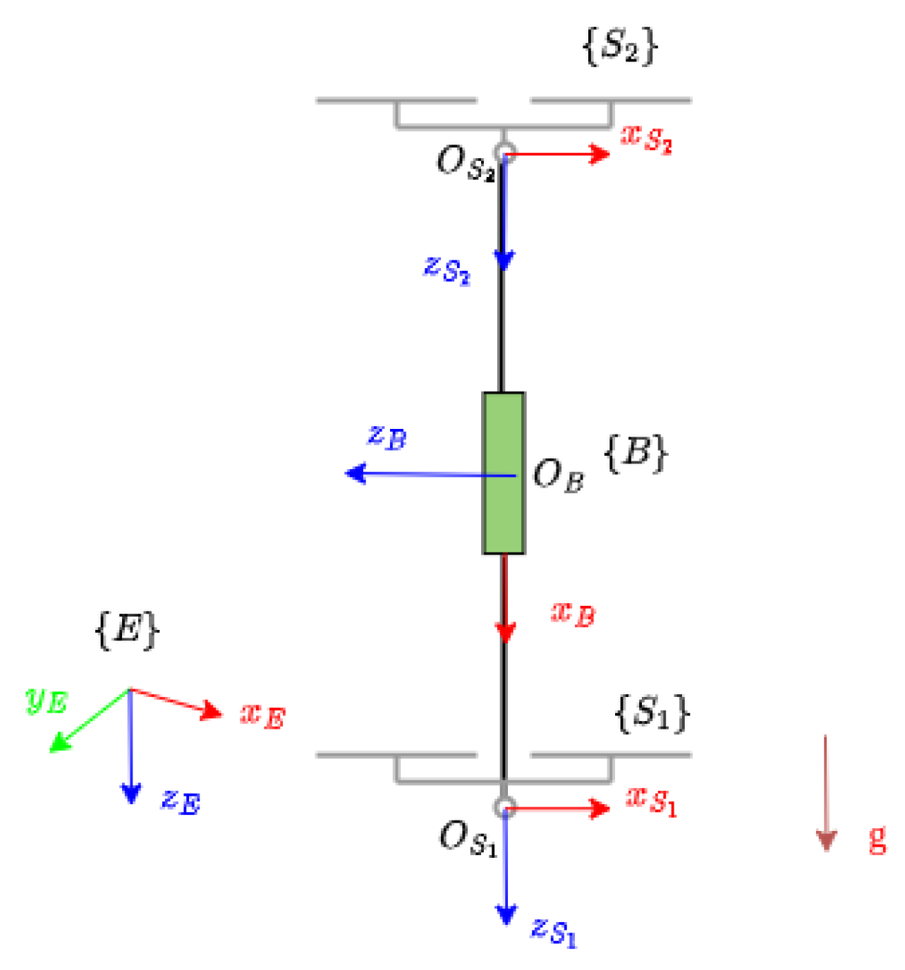
2.1. System Description and Modeling

Unlike traditional quadrotor systems, which typically provide 4 DOF in control inputs—namely, one thrust and three torques—this paper investigates a 5-DOF aerial platform, as illustrated in Figure 1. The control input of this platform includes a 5-DOF force/torque combination, consisting of three independent torques and two-dimensional forces. As a result, in the proposed 5-DOF aerial platforms, the rotational DOF around the body frame x axis is not independently controllable. It is inherently coupled with the translational motion due to the system’s actuation structure. In order to move along the y axis in the body frame, the system should rotate around the x axis to obtain a force in this direction.

Modeling Assumptions

The following assumptions are made in the derivation of the system dynamics:

• The aerial platform is treated as a rigid body with known mass and inertia;
• Aerodynamic effects such as drag and wind disturbances are neglected in the model.

To facilitate modeling, we define a body-fixed frame for the aircraft and express the force input $F_0$ and torque input ${\tau }_0$ in the body-fixed frame. Given the system’s 5-DOF nature, the force vector $F_0$ is constrained to lie in the $x\text{-}z$ plane of the body-fixed frame. As a result, the system dynamics can be formulated as follows:

$$M_s\dot{V}+C_s\left(V\right)+G_s=u$$

(1)

Here, $V=(v_0,{\omega }_0)$ denotes the body velocity of the vehicle, where $v_0\in {\mathbb{R}}^3$ and ${\omega }_0\in {\mathbb{R}}^3$ represent the linear and angular velocities in the body-fixed frame, respectively. The system input is given by $u=\left(F_0,{\tau }_0\right)$, where $F_0\in {\mathbb{R}}^3$ and ${\tau }_0\in {\mathbb{R}}^3$ are both expressed in the body-fixed frame. As $F_0$ is restricted in the $x\text{-}z$ plane of the body frame, it can be expressed as $F_0={(F_x,0,F_z)}^T$, where $F_x$ and $F_z$ represent the thrust along the x axis and z axis of the body frame. The mass matrix $M_s$, Coriolis term $C_s$, and gravity vector $G_s$ are given by

$$M_s=\left[\begin{array}{cc}m{I}_3& 0\\ 0& M_0\end{array}\right],C_s=\left[\begin{array}{c}{\widehat{\omega }}_{0}m{v}_0\\ {\widehat{\omega }}_0{M}_0{\omega }_0\end{array}\right],G_s=\left[\begin{array}{c}-R_0^{T}mg{e}_3\\ 0\end{array}\right]$$

where m is the total mass of the platform, $R_0\in SO\left(3\right)$ is the rotation matrix of the platform, $M_0\in {\mathbb{R}}^{3\times 3}$ is the inertia matrix, g is the gravitational acceleration, $e_3={(0,0,1)}^T$, $I_3$ is the identity matrix, and the hat map ${(·)}^{\wedge }:{\mathbb{R}}^3\to \mathfrak{so}\left(3\right)$ maps a vector $x\in {\mathbb{R}}^3$ to a skew-symmetric matrix such that $\widehat{x}y=x\times y$ for any $y\in {\mathbb{R}}^3$.

To complete the system description, the kinematic equations describing the evolution of the configuration variables are given as follows:

$${\dot{p}}_0=R_0{v}_0,{\dot{R}}_0=R_0{\widehat{\omega }}_0$$

(2)

Here, $p_0\in {\mathbb{R}}^3$ denotes the aircraft position in the inertial frame. These equations relate the body frame velocities $v_0$ and ${\omega }_0$ to the rates of change of the configuration variables in the inertial frame.

2.2. Flat Output Definition

A system is said to be differentially flat if there exists a set of outputs, known as flat outputs, such that all states and inputs of the system can be expressed as functions of these outputs and a finite number of their derivatives [40]. The flat output of a dynamical system is controllable, and the coordinates in the flat output space can typically be planned independently. For example, a traditional quadrotor system is differentially flat with respect to a four-dimensional flat output consisting of its position and yaw angle.

Unlike conventional quadrotors, the 5-DOF aerial platform considered in this work admits a five-dimensional flat output. We show that this flat output consists of the position and a subset of the system’s orientation—specifically, the yaw and pitch angles. The Z–Y–X Euler angle convention is adopted, where $\varphi$, $\theta$, and $\psi$ represent the roll, pitch, and yaw angles, respectively.

Lemma 1. 

Let $e_1={(1,0,0)}^T$, $e_2={(0,1,0)}^T$, and $e_3={(0,0,1)}^T$ be the orthogonal unit vectors corresponding to $x_B$, $y_B$, and $z_B$ of the frame $\left\{B\right\}$. Then, a fixed unit vector v lying in the $x_{B}O{z}_B$ plane can be expressed as $v=cos\theta e_1+sin\theta e_3$, where θ serves as a parameter. Then, for any rotation matrix $R\in SO\left(3\right)$, there exists a triple $(\alpha ,\beta ,\gamma )\in {[0,2\pi )}^3$ such that

$$R=exp\left(\alpha {\widehat{e}}_3\right)exp\left(\beta {\widehat{e}}_2\right)exp\left(\gamma \widehat{v}\right).$$

Consequently, this sequence of three rotations parameterizes the entire special orthogonal group $SO\left(3\right)$.

Proof. 

The special orthogonal group $SO\left(3\right)$ is a compact, connected, three-dimensional Lie group, and any minimal parameterization of $SO\left(3\right)$ must include three independent parameters. Consider the ordered product of three rotation matrices: $R=exp\left(\alpha {\widehat{e}}_3\right)exp\left(\beta {\widehat{e}}_2\right)exp\left(\gamma \widehat{v}\right)$. As $\alpha$ and $\beta$ vary, the rotated frame spans all orientations in $SO\left(3\right)$, and the axis v—being fixed in the rotated body frame but not aligned with the intermediate y axis—ensures that the final rotation introduces a third independent DOF.

The set of such compositions is closed under multiplication and contains the identity, and their associated infinitesimal generators (Lie algebra elements) span $\mathfrak{so}\left(3\right)$ because the three axes involved are linearly independent at almost every configuration. Therefore, according to the Lie group–Lie algebra correspondence and the surjectivity of the exponential map on compact Lie groups, such a composition covers all of $SO\left(3\right)$. Hence, any element of $SO\left(3\right)$ can be expressed in the given form.    □

This lemma means that any rotation in the special orthogonal group $SO\left(3\right)$ can be expressed as a composition of three rotations: first, a rotation about the global z axis; second, a rotation about the new y axis (i.e., the y axis after the first rotation); and third, a rotation about a fixed unit vector lying in the $x\text{-}z$ plane of the new coordinate frame.

Theorem 1. 

$y_1=(p_0,\theta ,\psi )$ is a flat output of the dynamic system (1) and (2).

Proof. 

From the dynamics of the system, it is seen that

$$m{\ddot{p}}_0=R_0{F}_0+mg{e}_3$$

(3)

In order to prove this, we construct a (possibly time-varying) unit vector $z_1\in S^2$, lying in the $x\text{-}z$ plane of the body frame, satisfying $R_0{z}_1\ne -z_1$.

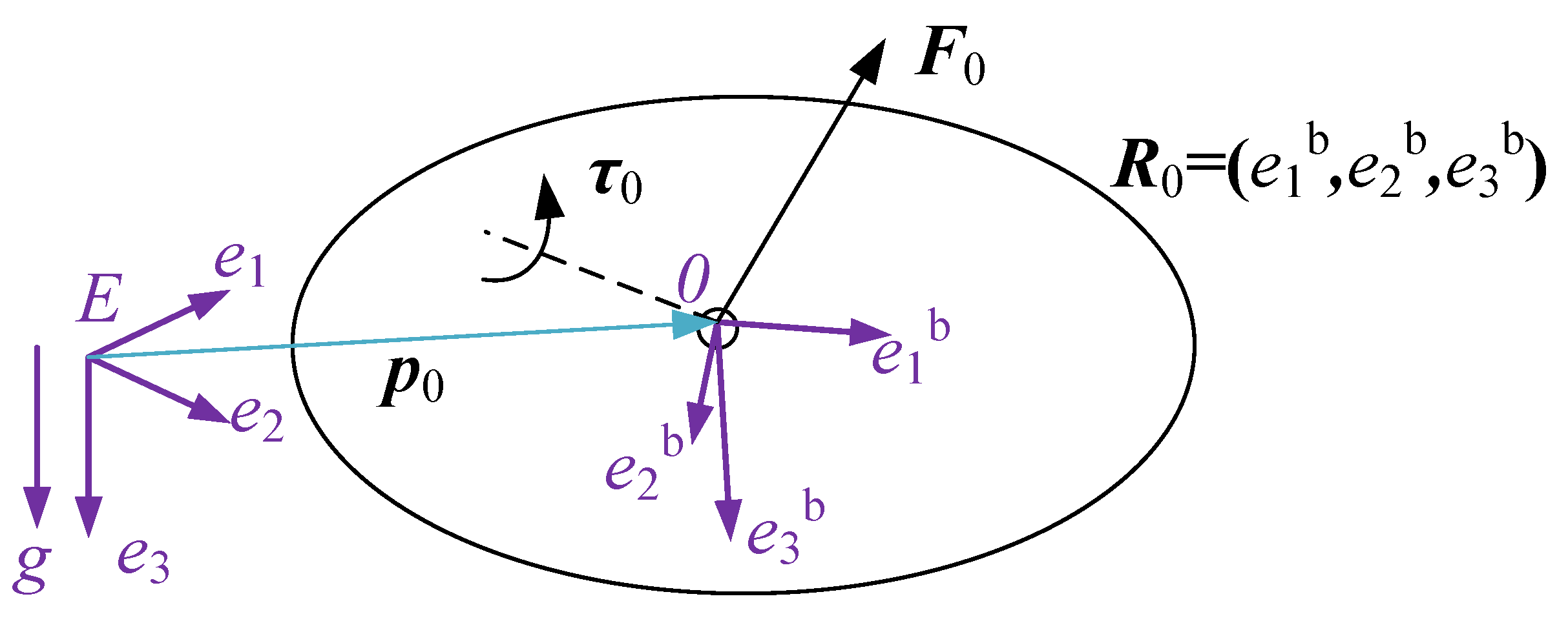
• According to Lemma 1, we can express the rotation matrix corresponding to attitude as

  $$R_0=exp\left(\psi {\widehat{e}}_3\right)exp\left(\theta {\widehat{e}}_2\right)exp\left(\overline{\varphi }{\widehat{z}}_1\right)$$

  (4)

  We express $R_{0,l}=exp\left(\psi {\widehat{e}}_3\right)exp\left(\theta {\widehat{e}}_2\right)$; then, we have

  $$exp\left(\overline{\varphi }{\widehat{z}}_1\right)F_0={R_{0,l}}^T(m{\ddot{p}}_0-mg{e}_3).$$

  (5)

  From $z_1$, one can obtain a unit vector $z_3$ in the $x\text{-}z$ plane such that $z_1·z_3=0$. It is evident that $F_0$ lies within the span of $z_1$ and $z_3$. If we assume that $\overline{\varphi }$ is not bounded, then based on the flat outputs $(R_{0,l},{\ddot{p}}_0)$, the input force $F_0$ can always be determined along the directions $z_1$ and $z_3$ as follows:

  $$\begin{array}{c}\langle F_0,z_1\rangle ={(m{\ddot{p}}_0-mg{e}_3)}^T{R}_{0,l}{z}_1\hfill \\ \langle F_0,z_3\rangle =\sqrt{\parallel R_{0,l}^T(m{\ddot{p}}_0-mg{e}_3){\parallel }^2-{\langle F_0,z_1\rangle }^2}\hfill \end{array}.$$

  (6)

  We introduce a rotation matrix $R_z=(z_1,z_3\times z_1,z_3)$. Since $z_1=R_z{e}_1$, we have

  $$exp\left(\overline{\varphi }{\widehat{z}}_1\right)=R_{z}exp\left(\overline{\varphi }{\widehat{e}}_1\right)R_z^T,F_0=R_z\left[\begin{array}{c}{F}_0^T{z}_1\\ 0\\ F_0^T{z}_3\end{array}\right]$$

  (7)

  Then, the force allocation in Equation (5) can be reformulated as

  $$R_{z}exp\left(\overline{\varphi }{\widehat{e}}_1\right)R_z^T{R}_z\left[\begin{array}{c}{F}_0^T{z}_1\\ 0\\ F_0^T{z}_3\end{array}\right]={R_{0,l}}^T(m{\ddot{p}}_0-mg{e}_3)$$

  (8)

  where $exp\left(\overline{\varphi }{\widehat{e}}_1\right)=(e_1,e_{2\varphi },e_{3\varphi })$. Then, the components can be computed as

  $$e_{3\varphi }={\displaystyle \frac{R_z^T{R}_{0,l}^T(m{\ddot{p}}_0-mg{e}_3)-\left(F_0^T{z}_1\right)e_1}{F_0^T{z}_3}},F_0^T{z}_3\ne 0$$

  (9)

  and $e_{2\varphi }=e_{3\varphi }\times e_1$. Therefore, the attitude matrix of the vehicle base is obtained by

  $$R_0=R_{0,l}{R}_{z}exp\left(\overline{\varphi }{\widehat{e}}_1\right)R_z^T.$$

  (10)

  Then, the input $F_0$ can be further derived using the following equation:

  $$F_0=R_0^T(m{\ddot{p}}_0-mg{e}_3)$$

  (11)

  However, it should be noted that if $F_0^T{z}_3=0$, a singularity in (9) occurs, and $e_{3\varphi }$ cannot be solved. To avoid this singularity, we propose an algorithm to modify $z_1$, i.e., to let $z_1$ point in the direction that maximizes $\langle F_0,z_3\rangle$. As maximizing $\langle F_0,z_3\rangle$ implies minimizing $\langle F_0,z_1\rangle$, the solution of $z_1$ can be expressed as

  $$\begin{array}{c}\underset{\begin{array}{c}{z}_1\end{array}}{min}{(m{\ddot{p}}_0-mg{e}_3)}^T{R}_{0,l}{z}_1\hfill \\ s.t.\left\{\begin{array}{c}{R}_0{z}_1\ne -z_1\hfill \\ z_1·e_2=0\hfill \end{array}\right.\hfill \end{array}$$

  (12)

  To obtain $z_1$ from (12), we first construct a local frame $\left\{L\right\}$ by rotating the inertial frame using $R_{0,l}$. We then project the vector $(m{\ddot{p}}_0-mg{e}_3)$ onto the $x\text{-}z$ plane of the local frame $\left\{L\right\}$, and we define $z_1$ to be perpendicular to this projected vector within the plane. To compute the desired direction in the local $x\text{-}z$ plane, we proceed as follows.
  Let $F_{\mathrm{nograv}}=(m{\ddot{p}}_0-mg{e}_3)$ be the force vector with the gravitational component removed. Note that it is expressed in the inertial frame. We project $F_{\mathrm{nograv}}$ onto the $x\text{-}z$ plane of $\left\{L\right\}$ by removing its component along the local y axis:

  $$F_{\mathrm{proj}}=F_{\mathrm{nograv}}-\left({\left(R_{0,l}{e}_2\right)}^T{F}_{\mathrm{nograv}}\right)\left(R_{0,l}{e}_2\right).$$

  (13)

  The components of $F_{\mathrm{proj}}$ along the x- and z-axes of $\left\{L\right\}$ are computed as

  $$a_x={\left(R_{0,l}{e}_1\right)}^T{F}_{\mathrm{proj}},a_z={\left(R_{0,l}{e}_3\right)}^T{F}_{\mathrm{proj}}.$$

  (14)

  We then construct a vector normal to $F_{\mathrm{proj}}$ in the $x\text{-}z$ plane

  $$v_{\mathrm{normal}}=-a_z·\left(R_{0,l}{e}_1\right)+a_x·\left(R_{0,l}{e}_3\right)$$

  (15)

  which is expressed in the inertial frame.
• This vector is normalized to obtain a unit direction:

  $$v_{\mathrm{normal}}^{\mathrm{unit}}={\displaystyle \frac{v_{\mathrm{normal}}}{\parallel v_{\mathrm{normal}}\parallel }}.$$

  (16)

  We then express this unit vector in the local coordinate frame $\left\{L\right\}$:

  $$v_{\mathrm{normal}}^{\mathrm{local}}=R_{0,l}^T{v}_{\mathrm{normal}}^{\mathrm{unit}}.$$

  (17)

  This local vector is then used as the solution to $z_1$

  $$z_1=v_{\mathrm{normal}}^{\mathrm{local}}.$$

  (18)

  Equations (13)–(18) together define a consistent method to extract and reorient the direction of interest in the local $x\text{-}z$ plane. It is seen that this is the solution of (12).
  The angular velocity can be expressed in terms of the rotation matrix as

  $${\widehat{\omega }}_0=R_0^T{\dot{R}}_0$$

  (19)

  Since $R_0$ is a function of $y_1$ and a finite number of its derivatives, it follows that ${\omega }_0$ can also be expressed as a function of $y_1$ and a finite number of its derivatives.
• Moreover, because ${\tau }_0\in {\mathbb{R}}^3$, the rotational system is fully actuated, and it is seen that ${\tau }_0=M_0{\dot{\omega }}_0+{\widehat{\omega }}_0{M}_0{\omega }_0$. Therefore, ${\tau }_0$ can also be derived as the function of $y_1$ and a finite number of its derivatives. For brevity, the detailed derivation is omitted here, as it does not affect the validity of the proof.
• By now, it is seen that all the states and inputs of the system can be expressed as functions of $y_1$ and the finite number of its derivatives. The proof that $y_1$ is the flat output is, thus, complete. Furthermore, by designing $z_1$ in this proof, the input and state can always be derived from finite-order derivatives of the flat output.    □

Remark 1. 

From the proof procedure, it is seen that the derivation of $R_0$ from $y_1$ is globally valid by appropriately varying $z_1$. This differs from the approach in the previous work [37]. This property can be exploited to design a singularity-free control allocation scheme, which is a key component of the controller for this class of systems.

3. Global Control Design and Stability Analysis

The control problem for the proposed 5-DOF aerial system can be formulated as follows.

Problem 1. 

Based on the system model described in (1) and (2) and a reference flat output trajectory

$$y_{1,d}=(p_{0,d},{\theta }_d,{\psi }_d):t\mapsto y_{1,d}\left(t\right)\in {\mathbb{R}}^5,$$

design a control input u such that the system output $y_1$ converges to the reference $y_{1,d}$ along the trajectory governed by (1) and (2).

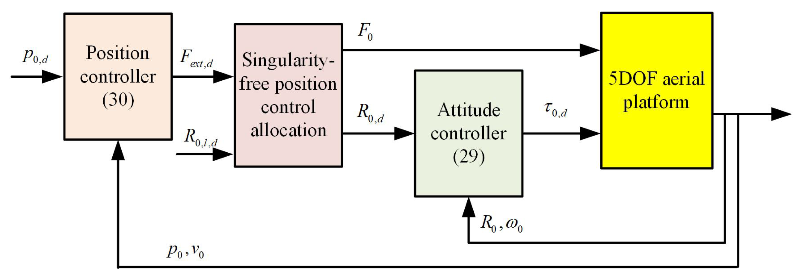
3.1. Control Strategy

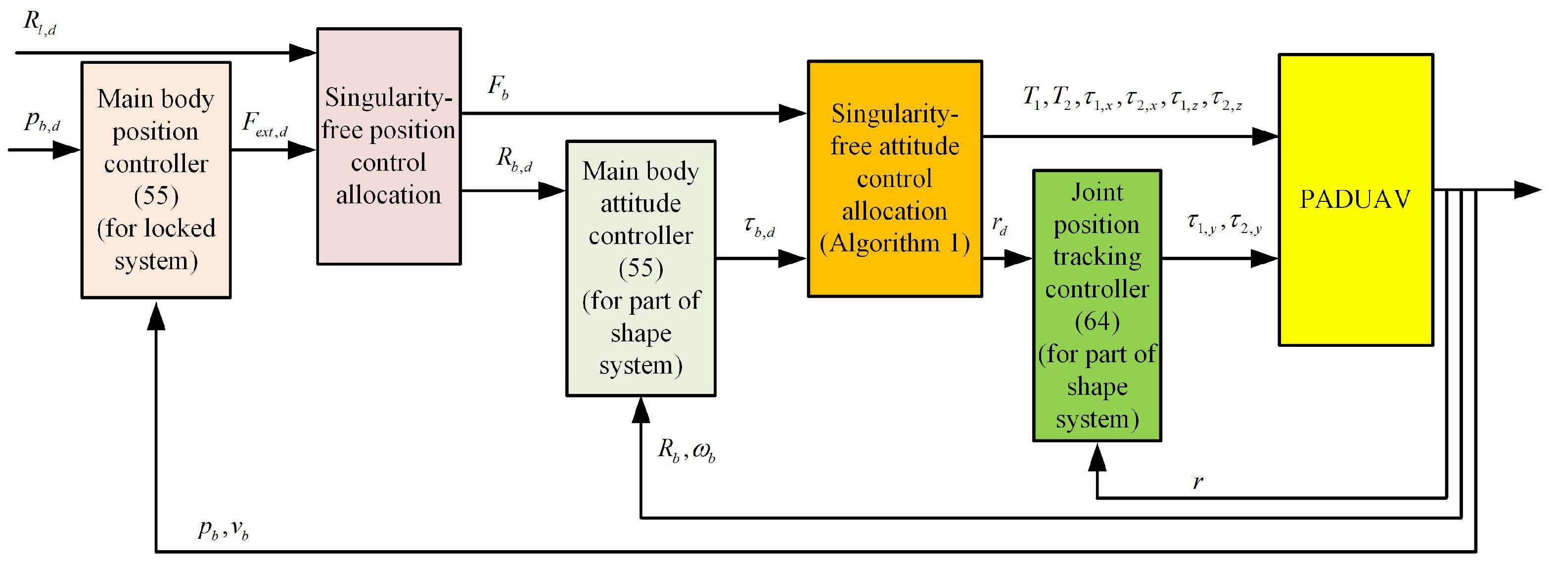
Overall Control Architecture

From Theorem 1, it is evident that the entire 5-DOF platform system is underactuated, while the rotational subsystem is fully actuated. The overall control architecture consists of an outer loop controller and an inner loop controller. Since the proposed 5-DOF system tracks 3D position and 2D attitude, the general control framework is illustrated in Figure 5.

The control allocation module connecting the position controller and the attitude controller requires careful design. The outer loop controller outputs the desired force, so it is critical for the connecting module to compute the corresponding desired attitude from this desired force. Based on Theorem 1 the desired rotation matrix can be decomposed into $z_1$ and $R_l$. Then, following the steps in the proof of Proposition 2, the desired force and attitude can be obtained accordingly.

3.2. Attitude Tracking Controller

We adopt the attitude tracking controller proposed in [4], which guarantees global and fast convergence of the attitude tracking error. The attitude is represented using exponential coordinates, and a hybrid formulation of the rotational dynamics is developed based on hybrid systems theory. This formulation is chosen because it effectively captures the geometric properties of the attitude error on $SO\left(3\right)$, as illustrated in Lemma 1 of [4].

The exponential map arises naturally from the structure of Lie groups, as discussed in [41,42]. The special orthogonal group $SO\left(3\right)$, which describes rigid body rotations, is a specific subgroup within the broader general linear group $GL\left(n\right)$. For elements in $GL\left(n\right)$, the exponential map corresponds directly to the standard matrix exponential operation [41]

$$exp\left(\widehat{\xi }\right)=I+sin\left(\parallel \xi \parallel \right){\displaystyle \frac{\widehat{\xi }}{\parallel \xi \parallel }}+{\displaystyle \frac{{\widehat{\xi }}^2}{{\parallel \xi \parallel }^2}}\left[1-cos\left(\parallel \xi \parallel \right)\right]$$

(20)

Here, I is the identity matrix, $\widehat{\xi }\in \mathfrak{so}\left(3\right)$ represents an element of the Lie algebra associated with the rotation group $SO\left(3\right)$. Conversely, for any rotation matrix $R\in SO\left(3\right)$, one can define a vector $\xi \in {\mathbb{R}}^3$ such that $R=exp\left(\widehat{\xi }\right)$. This vector $\xi$ is referred to as the exponential coordinates of the rotation matrix R.

Taking the derivative of (20) leads to the resulting expression shown below [41]

$${\displaystyle \frac{d}{dt}}exp\left(\widehat{\xi }\left(t\right)\right)=exp\left(\widehat{\xi }\left(t\right)\right){\left(dexp\left(-\xi \left(t\right)\right)\dot{\xi }\left(t\right)\right)}^{^}$$

(21)

An explicit closed-form representation is available, as shown in [41]:

$$dexp\left(\xi \right)=I+{\displaystyle \frac{S^2}{2}}\widehat{\xi }+{\displaystyle \frac{1-Scos(\parallel \xi \parallel /2)}{{\parallel \xi \parallel }^2}}{\widehat{\xi }}^2$$

(22)

where $S=sin\left(\parallel \xi \parallel /2\right)/\left(\parallel \xi \parallel /2\right)$. In the special case where $\xi =0$, both the differential of the exponential map and its inverse reduce to the identity matrix: $dexp\left(\xi \right)={dexp}^{-1}\left(\xi \right)=I$.

By analyzing the differential of the exponential map, a relationship can be established between the tangent vector $\dot{\xi }\in {\mathbb{R}}^3$ and the angular velocity $\omega \in {\mathbb{R}}^3$. Incorporating Equation (21) into the rigid body’s attitude kinematics leads to the following result:

$$\dot{\xi }=J_a\left(\xi \right)\omega$$

(23)

where $J_a\left(\xi \right)={dexp}^{-1}\left(-\xi \left(t\right)\right)$. This matrix remains invertible as long as $\xi$ is confined within the ball $B_a=\{\xi \in {\mathbb{R}}^3:\parallel \xi \parallel \le a\}$, where a is a constant satisfying $\pi \le a<2\pi$. This observation suggests that by carefully selecting the domain of $\xi$, representation singularities can be avoided.

Therefore, the rotational equation of motion of the aerial vehicle can be formulated within a hybrid framework as follows

$$\mathcal{H}:\left\{\begin{array}{c}\left\{\begin{array}{c}{\dot{\xi }}_0=J_a\left({\xi }_0\right){\omega }_0\hfill \\ {\dot{\omega }}_0=M_0^{-1}\left({\tau }_0-{\widehat{\omega }}_0{M}_0{\omega }_0\right)\hfill \end{array}\right.,\left({\xi }_0,{\omega }_0\right)\in S_C\hfill \\ \left\{\begin{array}{c}{\xi }_0^{+}={\xi }_0^{-}-2\pi {\displaystyle \frac{{\xi }_0^{-}}{\parallel {\xi }_0^{-}\parallel }}\hfill \\ {\omega }_0^{+}={\omega }_0^{-}\hfill \end{array}\right.,\left({\xi }_0,{\omega }_0\right)\in S_D\hfill \end{array}\right.$$

(24)

Given the flow set $S_C$ and the jump set $S_D$, they are defined as follows:

$$\begin{array}{c}{S}_D=\left\{({\xi }_0,{\omega }_0):\left|\right|{\xi }_0\left|\right|=a,〈{\dot{\xi }}_0,{\xi }_0〉>0\right\}\hfill \\ S_C=\left\{({\xi }_0,{\omega }_0):({\xi }_0,{\omega }_0)\notin S_D\right\}\hfill \end{array}$$

(25)

where ${\xi }_0$ denotes the exponential coordinates associated with the rotation matrix $R_0$. It is constrained within a ball $B_a=\{\xi \in {\mathbb{R}}^3:\parallel \xi \parallel \le a,\pi \le a<2\pi \}$.

Based on (24), the equation of motion describing the rotational tracking error in terms of ${\xi }_0$ can be formulated as follows:

$$\begin{array}{c}\left\{\begin{array}{c}{\dot{\xi }}_e=J_a\left({\xi }_e\right){\omega }_e\hfill \\ {\dot{\omega }}_e=\phi ({\tau }_0,{\omega }_e,{\xi }_e,R_{0,d},{\dot{R}}_{0,d},{\ddot{R}}_{0,d})\hfill \end{array}\right.,\left({\xi }_e,{\omega }_e\right)\in S_C\hfill \\ \left\{\begin{array}{c}{\xi }_e^{+}={\xi }_e^{-}-{\displaystyle \frac{2\pi }{a}}{\xi }_e^{-}\hfill \\ {\omega }_e^{+}={\omega }_e^{-}\hfill \end{array}\right.,\left({\xi }_e,{\omega }_e\right)\in S_D\hfill \end{array},$$

(26)

Here, we define the attitude tracking error ${\xi }_e$ via the relation $exp\left({\widehat{\xi }}_e\right)=R_{0,d}^T{R}_0:=R_e$, where $R_{0,d}$ represents the desired rotation matrix. The angular velocity tracking error is given by ${\omega }_e={\omega }_0-{\omega }_{0,d}$, where ${\omega }_{0,d}$ denotes the desired angular velocity. The expression of $\phi (·)$ is given as

$$\begin{array}{cc}\hfill \phi (·)& =M_0^{-1}[{\tau }_0-\left({\widehat{\omega }}_e+exp(-{\widehat{\xi }}_e){\widehat{\omega }}_{0,d}exp\left({\widehat{\xi }}_e\right)\right)M_0\left({\omega }_e+exp(-{\widehat{\xi }}_e){\omega }_{0,d}\right)]+\hfill \\ \hfill & \left({\widehat{\omega }}_e+exp(-{\widehat{\xi }}_e){\widehat{\omega }}_{0,d}exp\left({\widehat{\xi }}_e\right)\right)exp(-{\widehat{\xi }}_e){\omega }_{0,d}-exp(-{\widehat{\xi }}_e){\dot{\omega }}_{0,d}\hfill \end{array}$$

In practical implementations, especially under real-time conditions, sensor and estimation noise may induce undesired chattering in hybrid control systems. To mitigate this effect, the domain of ${\xi }_e$ is redefined as

$${\Omega }_{{\xi }_e}=\left\{{\xi }_e\in {\mathbb{R}}^3:\parallel {\xi }_e\parallel \le \pi +\delta \right\}:=B_{\pi +\delta }$$

(27)

where $\delta$ is a small positive threshold introduced to mitigate sensitivity to noise in the vicinity of the boundary.

Accordingly, the switching surface $S_D$ associated with ${\xi }_e$ is updated as follows:

$$S_D=\left\{{\xi }_e\in B_{\pi +\delta }:\parallel {\xi }_e\parallel =\pi +\delta ,\langle {\omega }_e,{\xi }_e\rangle >0\right\}.$$

(28)

Recasting the problem in terms of tracking error dynamics, the objective of global rotational tracking reduces to stabilizing the system described in (26) at the origin $({\xi }_e,{\dot{\xi }}_e)=(0,0)$. To this end, we introduce the control strategy as [4]

$${\tau }_{0,d}=-k_{\xi }{\xi }_e-k_{\omega }{\omega }_e-M_0\left({\widehat{\omega }}_{0}exp(-{\widehat{\xi }}_e){\omega }_{0,d}-exp(-{\widehat{\xi }}_e){\dot{\omega }}_{0,d}\right)$$

(29)

where $k_{\xi }$ and $k_{\omega }$ are positive constants.

From the definition of the tracking error dynamics and the tracking controller, the following stability can be obtained.

Given the tracking error dynamics described in Equation (26) and the control input ${\tau }_{0,d}$ defined by (29), assume that the constants $k_{\xi }$ and $k_{\omega }$ are strictly positive. Under these assumptions, the system admits a unique equilibrium at $({\xi }_e,{\omega }_e)=(0,0)$, and this equilibrium is exponentially stable within the domain $\left(B_{\pi +\delta }\right)\times {\mathbb{R}}^3$. This stability is equivalent to exponential stability on $SO\left(3\right)\times {\mathbb{R}}^3$.

3.3. Position Controller

The position controller can be any exponentially stable controller designed based on the position subsystem. To facilitate control design, we introduce a virtual force input for the aerial system defined as $F_{\mathrm{ext},d}=mg{e}_3+R_{0,d}{F}_0\in {\mathbb{R}}^3$, where $R_{0,d}\in SO\left(3\right)$ denotes a smoothly commanded rotation matrix.

Then, the equations governing the translational motion can be reformulated as

$${\dot{p}}_0={\dot{p}}_0,{\ddot{p}}_0={\displaystyle \frac{F_{\mathrm{ext},d}}{m}}+\left({\displaystyle \frac{R_0{F}_0}{m}}-{\displaystyle \frac{R_{0,d}{F}_0}{m}}\right)$$

Given the desired position $p_{0,d}\in {\mathbb{R}}^3$, an example of such a controller is designed as

$$F_{ext,d}=m(-k_T{e}_l+{\ddot{p}}_{0,d})$$

(30)

Here, $e_l={\left[\begin{array}{cc}{p}_e^T& {\dot{p}}_e^T\end{array}\right]}^T$, where the position error is defined as $p_e=p_0-p_{0,d}$. The gain matrix $k_T=(k_p,k_v)\in {\mathbb{R}}^{3\times 6}$ consists of the positive definite diagonal matrices $k_p$ and $k_v$. It is important to note that the resulting force is represented in the inertial frame and accounts for the gravitational force.

3.4. Position Control Allocation

The position controller outputs the desired force, which must be converted into the corresponding desired attitude. This process, referred to as the force allocation module, can be carried out using the method presented in the proof of Theorem 1.

In the position control allocation, we can define $F_{\mathrm{nograv}}=(F_{ext,d}-mg{e}_3)$. Then, using the same procedures (13)–(18), one can obtain the desired $z_1$ and $z_3$ without any singularity.

Given the desired $R_{0,l,d}=exp\left({\psi }_d{\widehat{e}}_3\right)exp\left({\theta }_d{\widehat{e}}_2\right)$, then we can obtain the desired force along $z_1$ and $z_3$ as

$$\begin{array}{c}\langle F_0,z_1\rangle ={(F_{ext,d}-mg{e}_3)}^T{R}_{0,l,d}{z}_1\hfill \\ \langle F_0,z_3\rangle =\sqrt{\parallel R_{0,l,d}^T(F_{ext,d}-mg{e}_3){\parallel }^2-{\langle F_0,z_1\rangle }^2}\hfill \end{array}.$$

(31)

Then, derive $e_{3\varphi }$ as

$$e_{3\varphi }={\displaystyle \frac{R_z^T{R}_{0,l,d}^T(F_{ext,d}-mg{e}_3)-\left(F_0^T{z}_1\right)e_1}{F_0^T{z}_3}},F_0^T{z}_3\ne 0$$

Accordingly, the desired intermediate attitude can be represented as

$$exp\left(\overline{\varphi }{\widehat{e}}_1\right)=(e_1,e_{2\varphi },e_{3\varphi })$$

(32)

The desired attitude of the aircraft base is then given by

$$R_{0,d}=R_{0,l,d}{R}_{z}exp\left(\overline{\varphi }{\widehat{e}}_1\right)R_z^T.$$

(33)

Furthermore, the commanded thrust components along the body frame’s x axis and z axis can be expressed as

$$F_0=R_{0,d}^T(F_{ext,d}-mg{e}_3)$$

(34)

With this, the desired attitude and thrust of the main frame are fully determined based on the output of the position controller.

3.5. Stability Analysis

Lemma 2. 

[43] (Conditions for the Global Stability of the System in Cascade) Consider the following cascaded system

$${\dot{p}}_e=h(p_e,F_d,{\ddot{x}}_d)+\parallel \Delta (p_e,{\xi }_e)\parallel$$

(35)

Let $F_d=\alpha (p_e,{\ddot{x}}_d)$ be a stabilizing feedback for the non-connected subsystem ${\dot{p}}_e=h(p_e,F_d,{\ddot{x}}_d)$. Let $\tau =\beta ({\xi }_e,{\omega }_e,R_d)$ be any partial-state feedback such that the equilibrium point ${\xi }_e=0$ is globally asymptotically stable (GAS) and locally exponentially stable. Suppose that there exits a positive constant $c_1$ and one class-κ function $\gamma (.)$, differentiable at ${\xi }_e=0$, such that

$$\parallel \Delta (p_e,{\xi }_e)\parallel \le \gamma (\parallel {\xi }_e\parallel )\parallel p_e\parallel \mathit{for}\parallel p_e\parallel \ge c_1$$

If there exists a positive semi-definite radially unbounded function $V\left(p_e\right)$ and positive constants $c_2$ and $c_3$ such that, for $\parallel p_e\parallel \ge c_2$,

$$\left\{\begin{array}{c}{\displaystyle \frac{\partial V}{\partial p_e}}h\left(p_e,\alpha (p_e,\ddot{x})\right)\le 0\hfill \\ \parallel {\displaystyle \frac{\partial V}{\partial p_e}}\parallel \parallel p_e\parallel \le c_{3}V\left(p_e\right)\hfill \end{array}\right.$$

then the feedbacks $F_d=\alpha (p_e,{\ddot{x}}_d)$ and $\tau =\beta ({\xi }_e,{\omega }_e,R_d)$ guarantee the boundedness of all the solutions of (9). Furthermore, if ${\dot{p}}_e=h(p_e,\alpha (p_e,\ddot{x}))$ is GAS, then the equilibrium point $(p_e,{\xi }_e)=(0,0)$ is GAS.

Proof. 

See [43].    □

Theorem 2. 

Assume the system evolves according to the dynamics in (1) and is provided with a continuously differentiable desired trajectory $y_{2,d}=(p_{0,d},R_{0,l,d})$. The control inputs are designed based on (29) and (30), where the desired attitude $R_{0,d}$ is derived from $(R_{0,l,d},F_d)$ according to (33). Under this control scheme, the system output $y_1$ is guaranteed to converge asymptotically to the reference trajectory $y_{1,d}$.

Proof. 

Taking into account the attitude tracking error $R_e$, the dynamics governing the position tracking error of the center of mass (COM) can be written as

$${\dot{e}}_l=\left[\begin{array}{cc}0& I\\ 0& 0\end{array}\right]e_l+\left[\begin{array}{c}0\\ I\end{array}\right]\left({\displaystyle \frac{F_{ext,d}}{m}}-{\ddot{p}}_{0,d}\right)+\left[\begin{array}{c}0\\ {\Delta }_p\end{array}\right].$$

(36)

Once $R_0$ converges to $R_{0,d}$ exponentially, it follows that ${\Delta }_p$ remains bounded, as established in [4].

• For the coupling term, we have

  $${\Delta }_p=-{\displaystyle \frac{R_{0,d}{F}_0}{m}}+{\displaystyle \frac{R_0{F}_0}{m}}=-{\displaystyle \frac{F_z}{m}}(R_{0,d}{e}_3-R_{0,d}{R}_e{e}_3)-{\displaystyle \frac{F_x}{m}}(R_{0,d}{e}_1-R_{0,d}{R}_e{e}_1)$$

  To finish the proof, we first prove the boundedness of $F_x$ and $F_z$, which is given in [43]

  $$|F_z|,|F_x|\le \left\{\begin{array}{c}{\kappa }_1\parallel p_e\parallel ,\mathrm{for}\parallel p_e\parallel \ge d\hfill \\ {\kappa }_{1}d,\mathrm{for}\parallel p_e\parallel <d\hfill \end{array}\right.$$

  (37)

  where ${\kappa }_1$ and d are positive constants.
• We now aim to establish that the term ${\displaystyle \frac{1}{m}}(R_{0,d}{e}_3-R_{0,d}{R}_e{e}_3)$ remains bounded. Specifically, we show that there exists a constant ${\kappa }_2>0$ such that

  $$\parallel R_{0,d}{e}_3-R_{0,d}{R}_e{e}_3\parallel \le {\kappa }_2\parallel {\xi }_e\parallel .$$

  (38)

  Since the 2-norm is submultiplicative and consistent with the vector norm, we can write

  $$\begin{array}{cc}\hfill \parallel R_{0,d}{e}_3-R_{0,d}{R}_e{e}_3\parallel & =\parallel R_{0,d}(I-R_e)e_3\parallel \hfill \\ \hfill & \le \parallel R_{0,d}{\parallel }_2\parallel I-R_e{\parallel }_2\parallel e_3\parallel .\hfill \end{array}$$

  (39)

  To bound $\parallel I-R_e{\parallel }_2$, we expand $R_e$ using Rodrigues’ formula:

  $$\begin{array}{cc}\hfill \parallel I-R_e{\parallel }_2& ={∥-{\displaystyle \frac{sin(\parallel {\xi }_e\parallel )}{\parallel {\xi }_e\parallel }}{\widehat{\xi }}_e-{\displaystyle \frac{1-cos(\parallel {\xi }_e\parallel )}{\parallel {\xi }_e{\parallel }^2}}{\widehat{\xi }}_e^2∥}_2\hfill \\ \hfill & \le {∥{\displaystyle \frac{sin(\parallel {\xi }_e\parallel )}{\parallel {\xi }_e\parallel }}I+{\displaystyle \frac{1-cos(\parallel {\xi }_e\parallel )}{\parallel {\xi }_e{\parallel }^2}}{\widehat{\xi }}_e∥}_2·{\parallel {\widehat{\xi }}_e\parallel }_2.\hfill \end{array}$$

  (40)

  We now estimate the second term on the right-hand side:

  $$\begin{array}{cc}\hfill {∥{\displaystyle \frac{1-cos(\parallel {\xi }_e\parallel )}{\parallel {\xi }_e{\parallel }^2}}{\widehat{\xi }}_e∥}_2& \le \left|{\displaystyle \frac{1-cos(\parallel {\xi }_e\parallel )}{\parallel {\xi }_e{\parallel }^2}}\right|·{\parallel {\widehat{\xi }}_e\parallel }_2\hfill \\ \hfill & =\left|{\displaystyle \frac{1-cos(\parallel {\xi }_e\parallel )}{\parallel {\xi }_e\parallel }}\right|·{\displaystyle \frac{\parallel {\widehat{\xi }}_e{\parallel }_2}{\parallel {\xi }_e\parallel }}.\hfill \end{array}$$

  Using the identity $\parallel {\widehat{\xi }}_e{\parallel }_2=\parallel {\xi }_e\parallel$, it follows that

  $${∥{\displaystyle \frac{1-cos(\parallel {\xi }_e\parallel )}{\parallel {\xi }_e{\parallel }^2}}{\widehat{\xi }}_e∥}_2\le \left|{\displaystyle \frac{1-cos(\parallel {\xi }_e\parallel )}{\parallel {\xi }_e\parallel }}\right|.$$

  Moreover, we note that

  $${∥{\displaystyle \frac{sin(\parallel {\xi }_e\parallel )}{\parallel {\xi }_e\parallel }}I∥}_2\le 1,\left|{\displaystyle \frac{1-cos(\parallel {\xi }_e\parallel )}{\parallel {\xi }_e\parallel }}\right|\le b,$$

  for some constant $b>0$. Substituting into (40), we obtain

  $$\parallel I-R_e{\parallel }_2\le (1+b)\parallel {\widehat{\xi }}_e{\parallel }_2\triangleq {\kappa }_2\parallel {\xi }_e\parallel .$$

  (41)

  This proved the inequality result of (38).
• Similarly, we can obtain that there exists a constant ${\kappa }_3>0$ such that

  $$\parallel R_{0,d}{e}_1-R_{0,d}{R}_e{e}_1\parallel \le {\kappa }_3\parallel {\xi }_e\parallel .$$

  (42)

  Finally, combining (37), (38), and (42), we obtain

  $$\parallel {\Delta }_p\parallel \le ({\kappa }_1{\kappa }_2+{\kappa }_1{\kappa }_3)\parallel {\xi }_e\parallel \parallel p_e\parallel \triangleq \mathcal{K}\left({\xi }_e\right)\parallel p_e\parallel ,\parallel p_e\parallel >d,$$

  (43)

  where $\mathcal{K}\left({\xi }_e\right)$ is a class-$\kappa$ function.
• Consequently, according to Lemma 2, the system described by (36) is stable at the equilibrium point $e_l=0$. Applying the stability results for cascade systems, it then follows that

  $$p_0\to p_{0,d},R_0\to R_{0,d}$$

  hold asymptotically for the entire system.    □

Remark 2. 

The controller design does not account for system perturbations. However, if the perturbations are bounded, a stable controller can ensure that the tracking error converges to a bounded region containing the origin. This result is formally stated in Lemma 9.2 of [44].

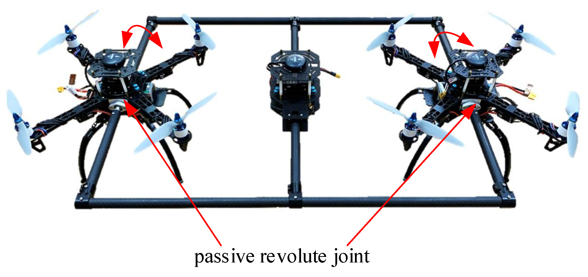
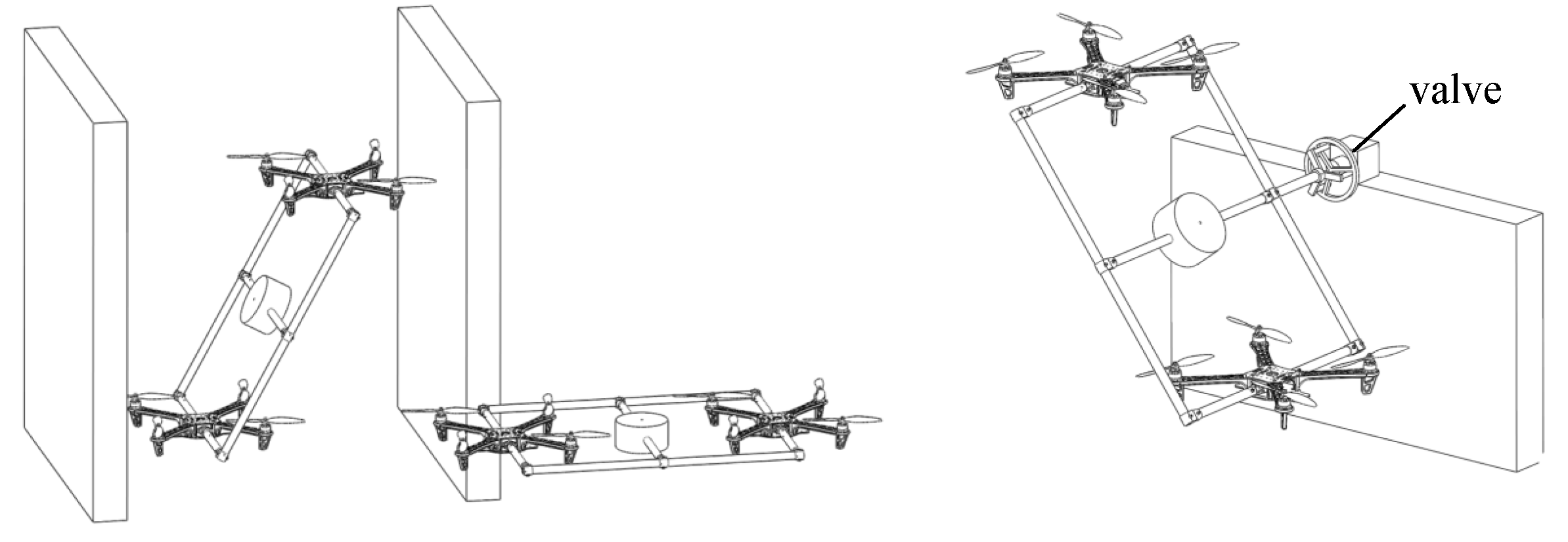
4. Applications on the PADUAV Platform

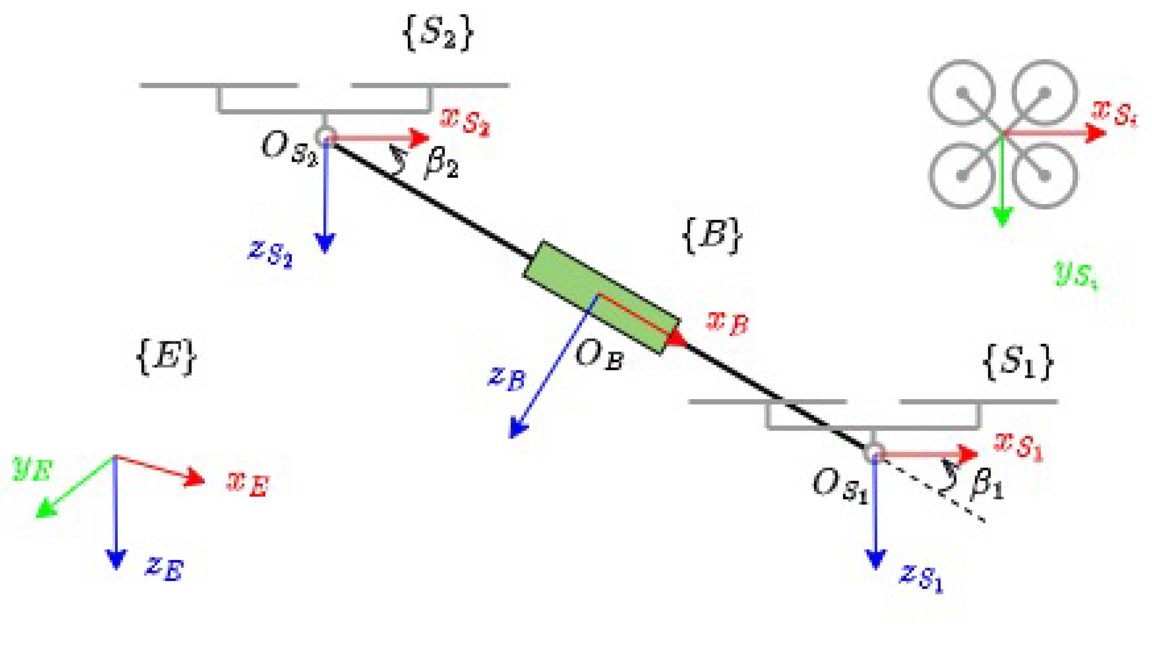
4.1. Configuration of the PADUAV Platform

The proposed PADUAV is a platform actuated by two off-the-shelf quadrotors, which will be referred to as ’subplanes’ in subsequent sections. These subplanes are passively articulated to a rigid frame. At the geometric center of the platform, a stack of carbon fiber disks, referred to as the center, accommodates the onboard computer, flight controller, GPS, battery, and any necessary operational tools. One prototype of such a platform is shown in Figure 2. As shown in Figure 6, the two quadrotors can provide thrust in the $x\text{-}z$ plane of the body-fixed frame, while combining the thrust of the two quadrotors results in 3D torque in the body-fixed frame. Therefore, the PADUAV is the kind of 5-DOF aircraft proposed in this paper.

As illustrated in Figure 6, the revolute joints are implemented using two specially designed bearing housings, allowing each subplane to pivot about the longitudinal side tubes. Unlike conventional tilting mechanisms that depend on servomotors to adjust rotor orientation, our approach uniquely employs fully functional quadrotors. These units independently produce both thrust and torque, enabling the tilting motion without additional actuation mechanisms.

It is important to highlight that both the central module and the two subplanes are powered independently, with no physical power lines linking them. This design ensures that, provided the subplanes communicate wirelessly with the onboard computer, there will be no cabling constraints that limit the range of tilting motion, which is an issue observed in [19,45]. From a practical standpoint, this setup is viable, as previous studies have demonstrated stable wireless communication between ground stations and multiple aerial vehicles. For instance, [24] employs XBee modules.

4.2. Dynamics Modeling

The motion of the PADUAV system consists of three components: the translational movement of the COM, the rotational dynamics of the main structure, and the relative axial rotation of the auxiliary units with respect to the main body.

The coordinate systems are depicted in Figure 6. The inertial reference frame is labeled as E, while a body-fixed frame B is attached to the center of the main body. Each auxiliary aerial module is equipped with its own local coordinate frame, denoted as $S_1$ and $S_2$. For each quadrotor (indexed by $i=1,2$), the thrust force is represented by the thrust $T_i\in \mathbb{R}$, and the torque generated is given by ${\tau }_i={({\tau }_{ix},{\tau }_{iy},{\tau }_{iz})}^T\in {\mathbb{R}}^3$.

Let ${}^{E}p_b={(x,y,z)}^{\mathrm{T}}\in {\mathbb{R}}^3$ denote the position of the main body with respect to the inertial frame $\left\{E\right\}$, and let $R_b\in \mathrm{SO}\left(3\right)$ represent its orientation. We define $r={[{\beta }_1,{\beta }_2]}^{\mathrm{T}}\in {\mathbb{R}}^2$ to represent the relative rotation angles between the quadrotor and the central body. Then, the full configuration of the system is compactly described by $H={(}^E{p}_b,R_b,r)\in {\mathbb{R}}^3\times \mathrm{SO}\left(3\right)\times {\mathbb{R}}^2$. The system velocity is represented by $\zeta ={(}^B{v}_b{,}^B{\omega }_b,\dot{r})\in {\mathbb{R}}^6\times {\mathbb{R}}^2$, where ${(}^B{v}_b{,}^B{\omega }_b)$ captures the linear and angular velocity of the main body expressed in its own frame. These configuration and velocity variables correspond directly to the three motion components previously outlined.

Assume the masses of subplane i and the main body are $m_i$ and $m_b$, the inertia of the subplane is $J_i=\mathrm{diag}\left([J_{ixx},J_{iyy},J_{izz}]\right)$, and that of the main body is $J_b$. Additionally, g represents gravitational acceleration.

By applying the Newton–Euler formalism, the equations governing the motion of the system can be systematically derived. The resulting dynamic model takes the following structured form [39]

$$\mathcal{M}\left(r\right)\dot{\zeta }+\mathcal{C}(r,\zeta )+\mathcal{G}(r,R_b)={}^B\tau _e$$

(44)

In this context, the equivalent input vector in configuration space is defined as ${}^B\tau _e=[{}^{B}F_b,{}^B\tau _b,n_{1y},n_{2y}]\in {\mathbb{R}}^8$, where ${}^{B}F_b\in {\mathbb{R}}^3$ is the equivalent force exerted on the main body, ${}^B\tau _b\in {\mathbb{R}}^3$ is the equivalent torque exerted on the main body, $n_{1y},n_{2y}$ is the equivalent joint torque. The dynamic model includes the mass matrix $\mathcal{M}\left(r\right)\in {\mathbb{R}}^{8\times 8}$, the combined centrifugal and Coriolis effects captured by $\mathcal{C}(r,\zeta )\in {\mathbb{R}}^8$, and the gravitational term $\mathcal{G}(r,R_b)\in {\mathbb{R}}^8$. It is important to note that these equivalent force and torque terms are derived by transforming the actual thrust and torques generated by the sub-quadrotors into a form compatible with the system’s configuration-space dynamics.

The equivalent input vector ${\tau }_e$ results from mapping the actual physical inputs $T_i$ and ${\tau }_i$ using the following force and moment relationships:

$$\begin{array}{cc}\hfill F_b& =F_1+F_2\hfill \\ \hfill {\tau }_b& ={\tau }_1+{\tau }_2-{\tau }_{1y}{y}_{S_1}-{\tau }_{2y}{y}_{S_2}+p_{c1}\times F_1+p_{c2}\times F_2\hfill \\ \hfill n_{iy}& ={\tau }_{iy}\hfill \end{array}$$

(45)

where $p_{ci}=\overrightarrow{O_B{O}_{Si}}$, $y_{S_i}$ is the unit vector of frame $\left\{S_i\right\}$. Given that the thrust vectors $F_1$ and $F_2$ from the two subcomponents are constrained to the x-z plane of the body-fixed frame B, it follows that ${}^{B}F_b={{[}^B{F}_{b,x},0{,}^B{F}_{b,z}]}^T$ and ${}^B\tau _b={{[}^B{\tau }_{b,x}{,}^B{\tau }_{b,y}{,}^B{\tau }_{b,z}]}^T$. This configuration implies that the system possesses five DOF.

4.3. Dynamics Analysis and Decoupling

Unlike the previous section, which focuses on a class of 5-DOF aerial vehicles, the proposed PADUAV platform exhibits more complex dynamics. The force and torque acting on the main body are generated by a pair of cooperating UAVs. To handle this complexity, we adopt the methodology from [46] to decouple the system dynamics. Specifically, the overall system is decomposed into a locked system and a shape system. The locked system represents the translational motion of the COM, while the shape system captures the rotational motion of the main body and the joint mechanisms.

4.3.1. Decouple the Translation Motion from General Rotations

To facilitate the analysis and control for this system, we decompose the tangent space associated with the dynamics in (44) using the passive decomposition framework proposed in [47], as follows:

$$\zeta =\left[\begin{array}{cc}{\Delta }_{\perp }& {\Delta }_{\top }\end{array}\right]\left[\begin{array}{c}{}^B\dot{p}_L\\ \mu \end{array}\right]:=\underset{S\left(r\right)}{\underbrace{\left[\begin{array}{cc}{I}_3& S_E\left(r\right)\\ 0& I_{n+3}\end{array}\right]}}\eta$$

(46)

Here, $\mu =\left({\omega }_b,\dot{r}\right)\in {\mathbb{R}}^5$ denotes the generalized velocity vector, and ${}^B\dot{p}_L$ represents the linear velocity of the center of mass of the entire system, expressed in the body-fixed frame $\left\{B\right\}$. The matrices $S_E\left(r\right)\in {\mathbb{R}}^{3\times 5}$ and $S\left(r\right)\in {\mathbb{R}}^{8\times 8}$ are configuration-dependent transformation matrices associated with the system’s dynamics.

By converting the linear velocity from the body frame, ${}^B\dot{p}_L$, to the inertial frame, the EOM can be reformulated in a decoupled structure as [47]

$$\begin{array}{cc}\hfill & \mathrm{locked}\mathrm{system}\left\{\begin{array}{c}{}^E\dot{p}_L={}^{E}v_L\hfill \\ m_L{}^E\dot{v}_L-m_{L}g{e}_3=R_b{}^{B}F_b\hfill \end{array}\right.\hfill \end{array}$$

(47)

$$\begin{array}{cc}\hfill & \mathrm{shape}\mathrm{system}\left\{\begin{array}{c}\dot{\sigma }=\sigma \widehat{\mu }\hfill \\ M_E\left(r\right)\dot{\mu }+C_E(r,\mu )=S_E^T{}^{B}F_b+\left[\begin{array}{c}{}^B\tau _b\\ n_{1y}\\ n_{2y}\end{array}\right]\stackrel{\Delta }{=}{}^B\tau _E\hfill \end{array}\right.\hfill \end{array}$$

(48)

Here, the total system mass is defined as $m_L:=m_b+m_1+m_2>0$. The generalized velocity vector is given by $\mu ={[}^B{\omega }_b;\dot{r}]$, while the configuration is compactly represented by $\sigma =(R_b,r)\in \mathrm{SO}\left(3\right)\times {\mathbb{R}}^2$. The transformed velocity is written as $\sigma \widehat{\mu }=(R_b^{\mathrm{T}}\widehat{{}^B\omega _b},\dot{r})$. For the shape subsystem, the matrices $M_E\left(r\right)\in {\mathbb{R}}^{5\times 5}$ and $C_E(r,\mu )\in {\mathbb{R}}^5$ correspond to the inertia and Coriolis/centrifugal terms.

Note that when $m_1=m_2$ and $p_{c1}=-p_{c2}$—i.e., the two quadrotors are identical—the COM of the entire system coincides with that of the main body. In this case, we have

$$p_L=p_b$$

(49)

4.3.2. Decoupling Main Body Rotation from Position and Joint Rotation

To facilitate controller design, the rotational motion of the main body and the joint dynamics can be further decoupled. Based on the kinematics, we obtain

$${}^{S_i}\dot{\omega }_{iy}={}^{S_i}\dot{\omega }_{by}+{\ddot{\beta }}_i$$

(50)

Define $\lambda ={{[}^{S_1}{\omega }_{1y},{}^{S_2}{\omega }_{2y}]}^{\mathrm{T}}$. Under this definition, the term $M_E\left(r\right)\dot{\mu }$ that appears in the shape subsystem dynamics can be reformulated as

$$\begin{array}{cc}\hfill M_E\left(r\right)\dot{\mu }=& \left[\begin{array}{c}{M}_{Er}{\left(r\right)}^B{\dot{\omega }}_b\\ J_{1yy}{(}^{S_1}{\dot{\omega }}_{by}+{\ddot{\beta }}_1)\\ J_{2yy}{(}^{S_2}{\dot{\omega }}_{by}+{\ddot{\beta }}_2)\end{array}\right]=\left[\begin{array}{c}{M}_{Er}{\left(r\right)}^B\dot{{\omega }_b}\\ {J_{1yy}}^{S_1}{\dot{\omega }}_{1y}\\ {J_{2yy}}^{S_2}{\dot{\omega }}_{2y}\end{array}\right]\hfill \\ \hfill =& \underset{:=M_E^{\prime }\left(r\right)}{\underbrace{\left[\begin{array}{cc}{M}_{Er}\left(r\right)& {\mathit{O}}_{3\times 2}\\ {\mathit{O}}_{2\times 3}& M_{yy}\end{array}\right]}}\left[\begin{array}{c}{\dot{\omega }}_b\\ \dot{\lambda }\end{array}\right]\hfill \end{array}$$

(51)

Here, $M_{Er}\left(r\right)\in {\mathbb{R}}^{3\times 3}$, and $M_{yy}=\mathrm{diag}(J_{1yy},J_{2yy})$. The matrices $M_E^{\prime }\left(r\right)$ and $C_E(r,\mu )$ take the following structured forms:

$$\begin{array}{cc}\hfill M_E^{\prime }\left(r\right)=& \left[\begin{array}{cc}{M}_{res}& {\mathit{O}}_{3\times 2}\\ {\mathit{O}}_{2\times 3}& M_{yy}\end{array}\right]\hfill \\ & +{\Sigma }_{i=1}^2(J_{ixx}-J_{izz})\left[\begin{array}{cc}{M}_{ixz}\left({\beta }_i\right)& {\mathit{O}}_{3\times 2}\\ {\mathit{O}}_{2\times 3}& {\mathit{O}}_{2\times 2}\end{array}\right]\hfill \end{array}$$

(52)

$$\begin{array}{cc}\hfill C_E(r,\mu )=& C_E(r,{}^B\omega _b,\dot{r})\hfill \\ \hfill =& \left[\begin{array}{c}{C}_{res}{(}^B{\omega }_b)\\ {\mathit{O}}_{2\times 1}\end{array}\right]+{\Sigma }_{i=1}^2{J}_{iyy}{C}_{iy}({\beta }_i,{\dot{\beta }}_i,{}^B\omega _b)\hfill \\ & +{\Sigma }_{i=1}^2(J_{ixx}-J_{izz})C_{ixz}({\beta }_i,{\dot{\beta }}_i,{}^B\omega _b)\hfill \end{array}$$

(53)

The subscript _res denotes the residual component, representing the remaining terms following the decoupling process.

When the conditions $\parallel J_{ixx}-J_{izz}\parallel =0$ and $J_{iyy}=0$ are met, the rotational dynamics of ${}^B\dot{\omega }_b$ and $\dot{\lambda }$ become fully independent and can be further decoupled.

Furthermore, if $m_1=m_2$ and $p_{c1}=-p_{c2}$—that is, the two quadrotors are identical—the resulting dynamics can be decoupled into two parts: one describing the rotational motion of the main body and the other governing the joint motion. These decoupled equations take the form

$$\begin{array}{cc}\hfill & M_{\mathrm{res}}{}^B\dot{\omega }_b+C_{\mathrm{res}}\left({}^B\omega _b\right)={}^B\tau _b\hfill \\ \hfill & M_{yy}\dot{\lambda }=\left[\begin{array}{c}{n}_{1y}\\ n_{2y}\end{array}\right]=\left[\begin{array}{c}{\tau }_{1y}\\ {\tau }_{2y}\end{array}\right]\hfill \end{array}$$

(54)

4.4. Controller Design

In this section, three sub-controllers are designed based on the three sets of decoupled dynamics introduced in Section 4.3. These sub-controllers are connected through linkage modules to form the overall control scheme, enabling stable tracking of the position in the x, y, and z directions, as well as the yaw and pitch motions of the proposed PADUAV platform. The overall control architecture is illustrated in Figure 7. In the proposed control framework, the position controller is developed based on the locked system dynamics in (47). The attitude controller is derived from the first equation of (54), while the joint tracking controller is constructed using the second equation of (54). The control allocation module is designed according to the formulation in (45).

To achieve 6-DOF maneuverability in the platform, we propose a 5-DOF geometric tracking control strategy based on the controller introduced in the previous section. This strategy consists of two cascaded sub-controller modules that independently track translational and rotational motions, respectively. Additional allocation modules are included to generate the desired force and attitude. Such mapping steps are essential due to the platform’s underactuation. The emphasis on the number of DOF highlights that this module group produces a 5-DOF output.

4.4.1. Position and Attitude Control of the Main Frame

Let $p_{L,d}$ denote the desired position, and let $R_{b,d}$ denote the desired rotation matrix. We define the position tracking errors $p_e=p_{L,d}-p_L$. The attitude tracking error ${\xi }_e$ is defined via the relation $exp\left({\dot{\xi }}_e\right)=R_{b,d}^T{R}_b:=R_e$. The angular velocity tracking error is given by ${\omega }_e={\omega }_b-{\omega }_{b,d}$, where ${\omega }_{b,d}$ defined by ${\widehat{\omega }}_{b,d}=R_{b,d}^T{\dot{R}}_{b,d}$ denotes the desired angular velocity. Based on the decoupled dynamics (47), the position and attitude tracking control laws are formulated as

$$\left\{\begin{array}{cc}{}^{E}F_{ext,d}\hfill & =m_L(-k_p{p}_e-k_v{\dot{p}}_e+{\ddot{p}}_{b,d})\hfill \\ {}^B\tau _{b,d}\hfill & =M_{res}(-k_{\xi }{\xi }_e-k_{\omega }{\omega }_e)+C_{res}\left({\omega }_b\right)\hfill \end{array}\right.$$

(55)

where $k_p$, $k_v$, $k_{\xi }$, and $k_{\omega }$ are positive constant gains. The commanded force is expressed in the earth frame $\left\{E\right\}$. The desired torque is expressed in the body frame $\left\{B\right\}$. Recall that $M_{res}$ and $C_{res}$ are defined in (52) and (53).

Given the desired force, and based on the proof of Theorem 1, we can now obtain the desired attitude and desired thrust from the desired force, which is the output of the position controller. The position control allocation follows the same procedure as that of the 5-DOF aerial platform described in the previous section.

4.4.2. Singularity-Free Attitude Control Allocation

If the system consists of two identical sub-aircraft, then the thrust allocation can be described by the following equations:

$$\begin{array}{c}-T_{2}sin{\beta }_2-T_{1}sin{\beta }_1{=}^B{F}_{b,x}\\ -T_{2}cos{\beta }_2-T_{1}cos{\beta }_1{=}^B{F}_{b,z}\\ T_1{p}_{1x}cos{\beta }_1-T_2{p}_{2x}cos{\beta }_2{=}^B{\tau }_{b,y}\end{array}$$

(56)

where $p_{ix}$ represents the constant distance from quadrotor-i to the COM of the entire system.

To compute the thrusts based on the desired force and torque acting on the main body, we define

$$-T_{i}sin{\beta }_i=T_{i,x},-T_{i}cos{\beta }_i=T_{i,z}$$

(57)

By substituting into Equation (56), we obtain

$$T_{1,z}={\displaystyle \frac{p_{1,x}{}^{B}F_{b,z}{-}^B{\tau }_{b,y}}{2p_{1,x}}},T_{2,z}={\displaystyle \frac{p_{1,x}{}^{B}F_{b,z}+{}^B\tau _{b,y}}{2p_{1,x}}}$$

(58)

To determine $T_{1,x}$ and $T_{2,x}$, a simple strategy is to assume

$$T_{1,x}=T_{2,x}={\displaystyle \frac{{}^{B}F_{b,x}}{2}}$$

(59)

Given the coordinate frame definitions, the angle between each sub-aircraft and the main frame is determined by

$${\beta }_{i,d}=\left\{\begin{array}{c}{tan}^{-1}{\displaystyle \frac{T_{i,x}}{T_{i,z}}}-\pi ,if{T}_{i,x}>0,T_{i,z}>0\\ {tan}^{-1}{\displaystyle \frac{T_{i,x}}{T_{i,z}}},else\end{array}\right.$$

(60)

To ensure smooth control actions, we minimize the change in the thrust direction angles between two consecutive time steps $k-1$ and k. Specifically, we define

$$\Delta {\beta }_i={\beta }_{i,d}\left(k\right)-{\beta }_{i,d}(k-1)$$

(61)

and formulate the following optimization to calculate $T_{i,x}$ instead of using (59),

$$\begin{array}{cc}\hfill & \underset{T_{1,x},T_{2,x}}{min}\sum _{i=1}^2{(\Delta {\beta }_i)}^2\hfill \\ \hfill & s.t.T_{1,x}+T_{2,x}={}^{B}F_{b,x}\hfill \end{array}$$

(62)

This objective encourages gradual changes in ${\beta }_{i,d}$.

Finally, the x- and z-components of the torque applied to each sub-aircraft are computed using the following transformation:

$${\tau }_{xz}=A^{†}\left[\begin{array}{c}{}^B\tau _{b,x}\\ {}^B\tau _{b,y}\end{array}\right]$$

(63)

where

$$A=\left[\begin{array}{cccc}cos\left({\beta }_1\right)& cos\left({\beta }_2\right)& sin\left({\beta }_1\right)& sin\left({\beta }_2\right)\\ -sin\left({\beta }_1\right)& -sin\left({\beta }_2\right)& cos\left({\beta }_1\right)& cos\left({\beta }_2\right)\end{array}\right]$$

and $A^{+}$ is the pseudo-inverse of A.

Based on the derivations above, the singularity-free thrust allocation algorithm is summarized in Algorithm 1.

Algorithm 1 Singularity-Free Thrust Allocation for Two Sub-Aircraft

Require:  Desired body force ${}^{B}F_b=[F_{b,x},F_{b,z}]$, torque ${}^B\tau _b=[{\tau }_{b,x},{\tau }_{b,y}]$, parameters $p_{1x},p_{2x}$, previous angles ${\beta }_1(k-1),{\beta }_2(k-1)$ Ensure:  Thrust magnitudes $T_1,T_2$, thrust directions ${\beta }_1,{\beta }_2$, sub-aircraft torques ${\tau }_{xz}$   1: Compute $T_{1,z}$ and $T_{2,z}$ using (58) 2: Compute $T_{1,x}$, $T_{2,x}$, ${\beta }_1$ and ${\beta }_2$ by minimizing angular variation: $$\underset{T_{1,x},T_{2,x}}{min}\sum _{i=1}^2{\left({\beta }_i\left(k\right)-{\beta }_i(k-1)\right)}^2\mathrm{s}.\mathrm{t}.T_{1,x}+T_{2,x}=F_{b,x}$$ 3: Compute $T_1$, $T_2$ using (57) 4: Compute ${\tau }_{xz}$ using (63) 5: return $T_1,T_2,{\beta }_1,{\beta }_2,{\tau }_{xz}$

4.4.3. Joint Position Tracking

The purpose of the joint position tracking controller is to ensure that the joint position follows the desired position output ${\beta }_{i,d}$ provided by the attitude control allocation. The joint position regulates the direction of the thrust generated by the two quadrotors, thereby adjusting the net thrust acting on the main frame of the PADUAV. The control torques ${\tau }_{1y}$ and ${\tau }_{2y}$ can be utilized to implement the joint position tracking controller.

First, define the tracking errors for the joint position and velocity as $e_{{\beta }_i}={\beta }_i-{\beta }_{i,d}$, ${\dot{e}}_{{\beta }_i}={\dot{\beta }}_i-{\dot{\beta }}_{i,d}$, The corresponding control input can then be designed as

$${\tau }_{i,y}=-k_{p\beta }{e}_{{\beta }_i}-k_{d\beta }{\dot{e}}_{{\beta }_i}$$

(64)

where $k_{p\beta }$ and $k_{d\beta }$ are positive constants.

Then, the commanded torque to each quadrotor can be calculated as

$${\tau }_{i,d}={({\tau }_{i,x},{\tau }_{i,y},{\tau }_{i,z})}^T$$

(65)

where ${\tau }_{i,x}$ and ${\tau }_{i,z}$ are the elements of ${\tau }_{xz}$, i.e., ${\tau }_{xz}={({\tau }_{1,x},{\tau }_{2,x},{\tau }_{1,z},{\tau }_{2,z})}^T$.

These computed torques and thrust instructions are subsequently dispatched to each module, where they are mapped into rotor speed commands. These actuation signals interact with the plant, guiding the system’s behavior in accordance with its inherent dynamics.

5. Numerical Simulation

The numerical simulation is carried out in MATLAB/SIMULINK 2016b incorporating the complete dynamics of the PADUAV model. The physical parameters of PADUAV in the simulation are summarized in

Table 1. Parameters of the PADUAV in the simulation.

Definition	Symbol	Value in Sim.
Mass of sub-quadrotor	$m_i$	1.251 kg
Inertia tensor of sub-quadrotor	$J_i$	0.0167 0.021 0.0167 kg · ${\mathrm{m}}^2$
Inertia tensor of the main body	$J_b$	0.019 0.021 0.039 kg · ${\mathrm{m}}^2$
distance of the center of the two sub-quadrotors	$p_{ix}$	0.4 m
Mass of the center stack	$m_b$	1.251 kg
Maximum thrust of each quadrotor	$T_{max}$	40 N

. These parameters come from the estimated parameters of a prototype of PADUAV.

To demonstrate the robustness of the proposed controller, sensor noise and time delays are introduced into the feedback loop. Specifically, a 0.01 s delay is added to the attitude and angular velocity feedback loop—representing the typical latency of onboard IMU sensors and filtering—while a 0.02 s delay is applied to the velocity and position feedback loop to reflect slower localization updates such as GPS. The joint position and angular velocity feedback is delayed by 0.01 s to simulate communication or processing latency.

The controller gains in the simulation are shown in

Table 2. Controller gains in the simulation.

Gain	Value
$k_p$	1.2
$k_v$	1.2
$k_{\xi }$	2.0
$k_{\omega }$	5.0
$k_{p\beta }$	2.0
$k_{d\beta }$	5.0

. Such gains were manually tuned through iterative simulations to balance tracking performance and robustness. We investigated the impact of varying control gains. Our results show that higher control gains generally reduce tracking error but may also increase sensitivity to external disturbances, potentially leading to instability. This trade-off highlights the importance of careful gain selection.

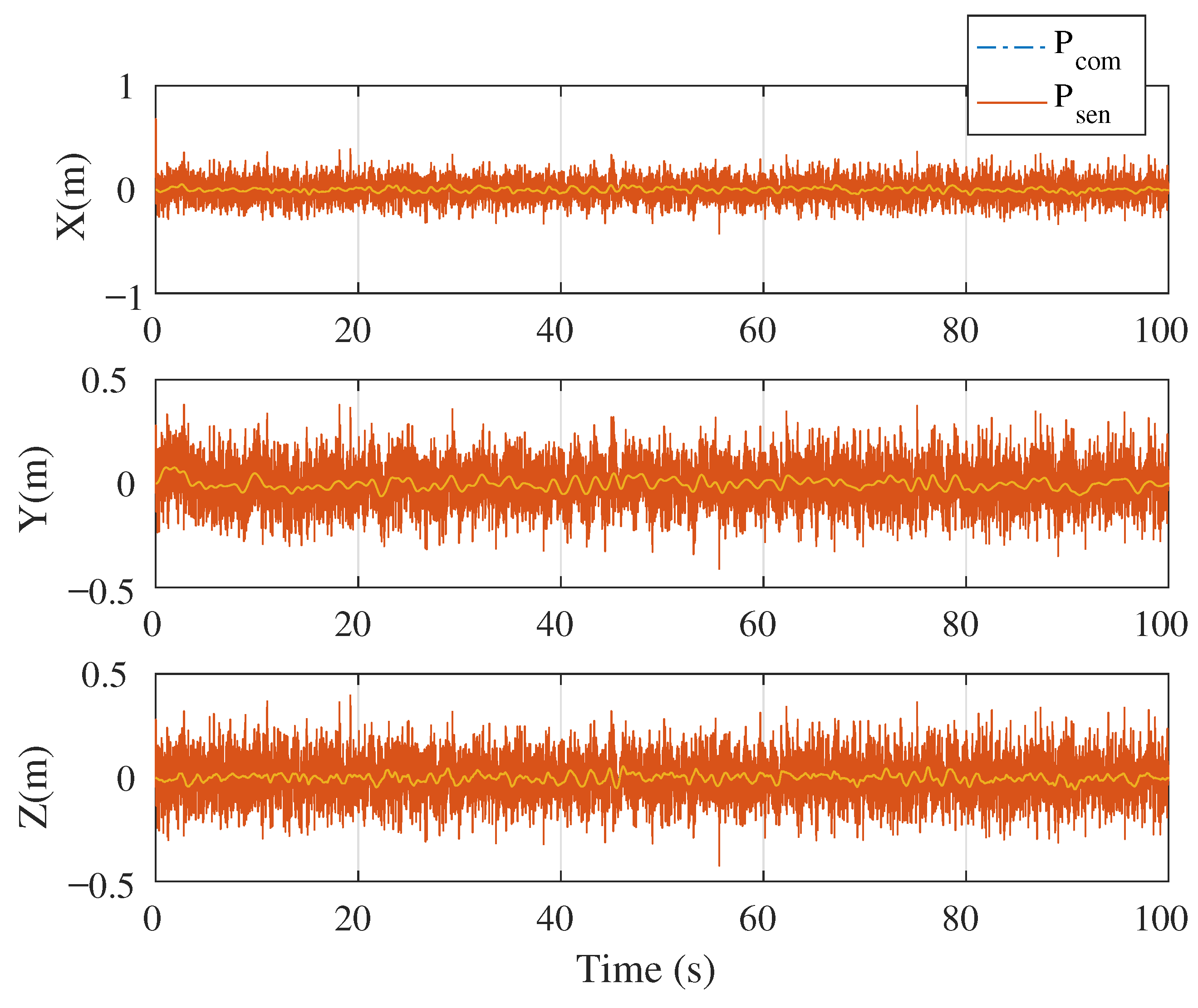
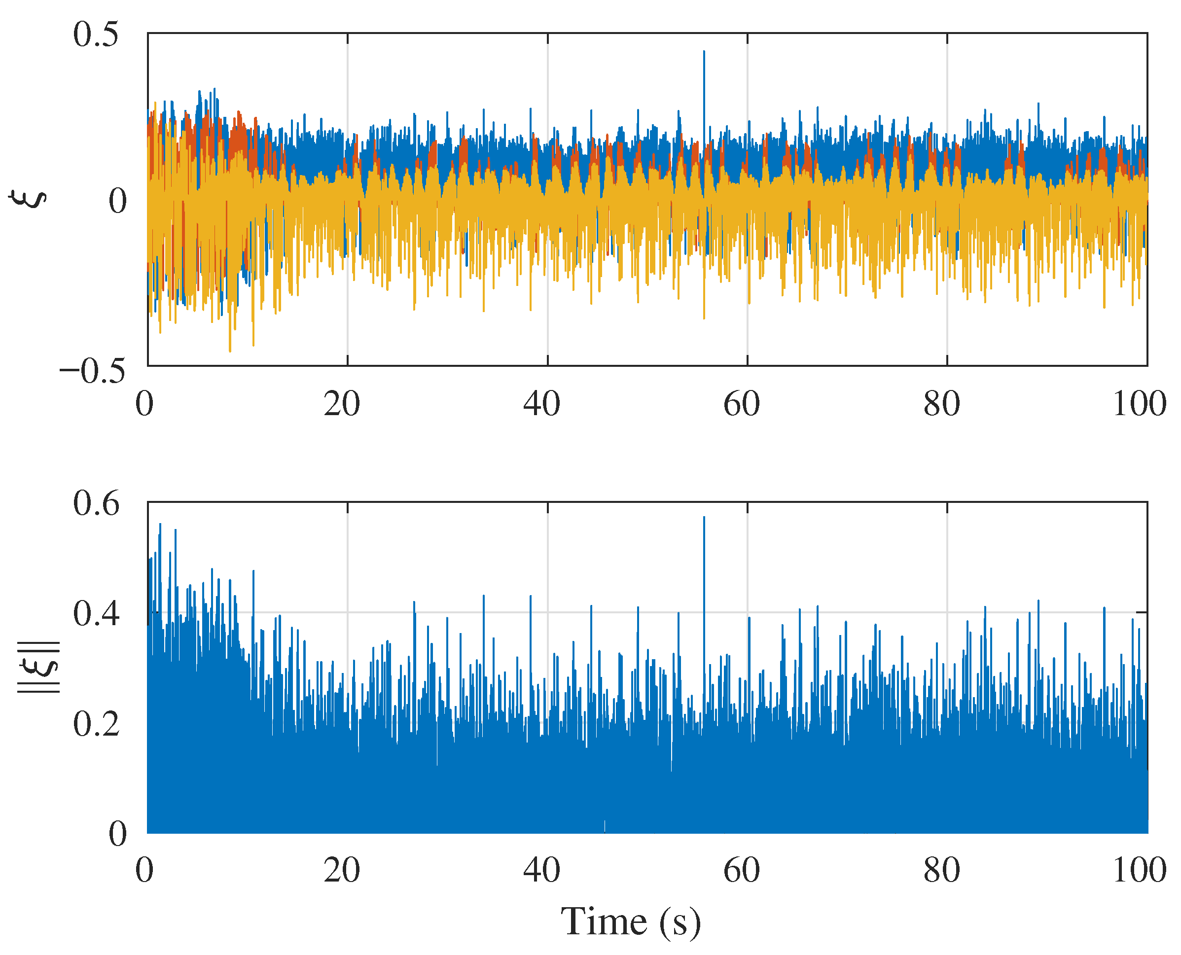
5.1. Simulation Case 1: Demonstration of Singularity-Free Capability

In the simulation, the main body of the PADUAV rotates about the body frame y axis and eventually stabilizes in a vertical attitude, which is a singular configuration, as shown in Figure 3. Throughout the simulation, the position of the main body remains unchanged. The control strategy proposed in this paper is used to govern the system’s behavior.

Figure 8 illustrates the position tracking performance of the main body, showing convergence to the desired trajectory. Figure 9 presents the attitude tracking results, demonstrating stable tracking that closely follows the desired orientation. These results confirm the system’s ability to maintain the singular configuration depicted in Figure 3. Note that the roll and yaw angles are confined to the interval $[-\pi ,\pi )$. Although the roll and pitch angles appear to exhibit discontinuities when the pitch angle approaches $\pi /2$, the actual attitude remains continuous. Figure 8 shows the linear position, representing the position of the locked system. This can be further verified in Figure 10, which shows the evolution of the attitude tracking error over time. The attitude is also plotted using a quaternion, as shown in Figure 11. It is evident that the attitude tracking error converges despite the presence of system uncertainties. Figure 9 and Figure 15 present the attitude and joint angles, representing the position of the shape system.

The control input signals (the thrust and torque for each quadrotor are shown in Figure 12) remain within feasible bounds throughout the task. Figure 13 shows the forces applied by the two quadrotors to the main body. Joint position tracking performance is presented in Figure 15, validating the accurate control of the two revolute joints. Figure 14 compares the equivalent torques generated by the two quadrotors, highlighting consistent dynamic compensation.

Figure 12. Control input (thrust and torque) provided by each quadrotor in simulation case 1.

Figure 12. Control input (thrust and torque) provided by each quadrotor in simulation case 1.

Figure 13. Equivalent desired force expressed in the inertial frame in simulation case 1.

Figure 13. Equivalent desired force expressed in the inertial frame in simulation case 1.

Figure 14. Equivalent torque on the main body in simulation case 1.

Figure 14. Equivalent torque on the main body in simulation case 1.

Figure 15. Joint position tracking in simulation case 1.

Figure 15. Joint position tracking in simulation case 1.

The observed noises in the simulation results are caused by persistent external disturbances applied to the system. As a result, the tracking error remains bounded instead of converging to the origin.

We investigated the impact of varying control gains. Our results show that higher control gains generally reduce tracking error but may also increase sensitivity to external disturbances, potentially leading to instability. This trade-off highlights the importance of careful gain selection.

For comparison, the controller proposed in [39] is also implemented in the simulation. However, it fails to stabilize the system when the main body approaches the singular configuration shown in Figure 3. In such cases where the baseline controller is employed, the system becomes uncontrollable or diverges.

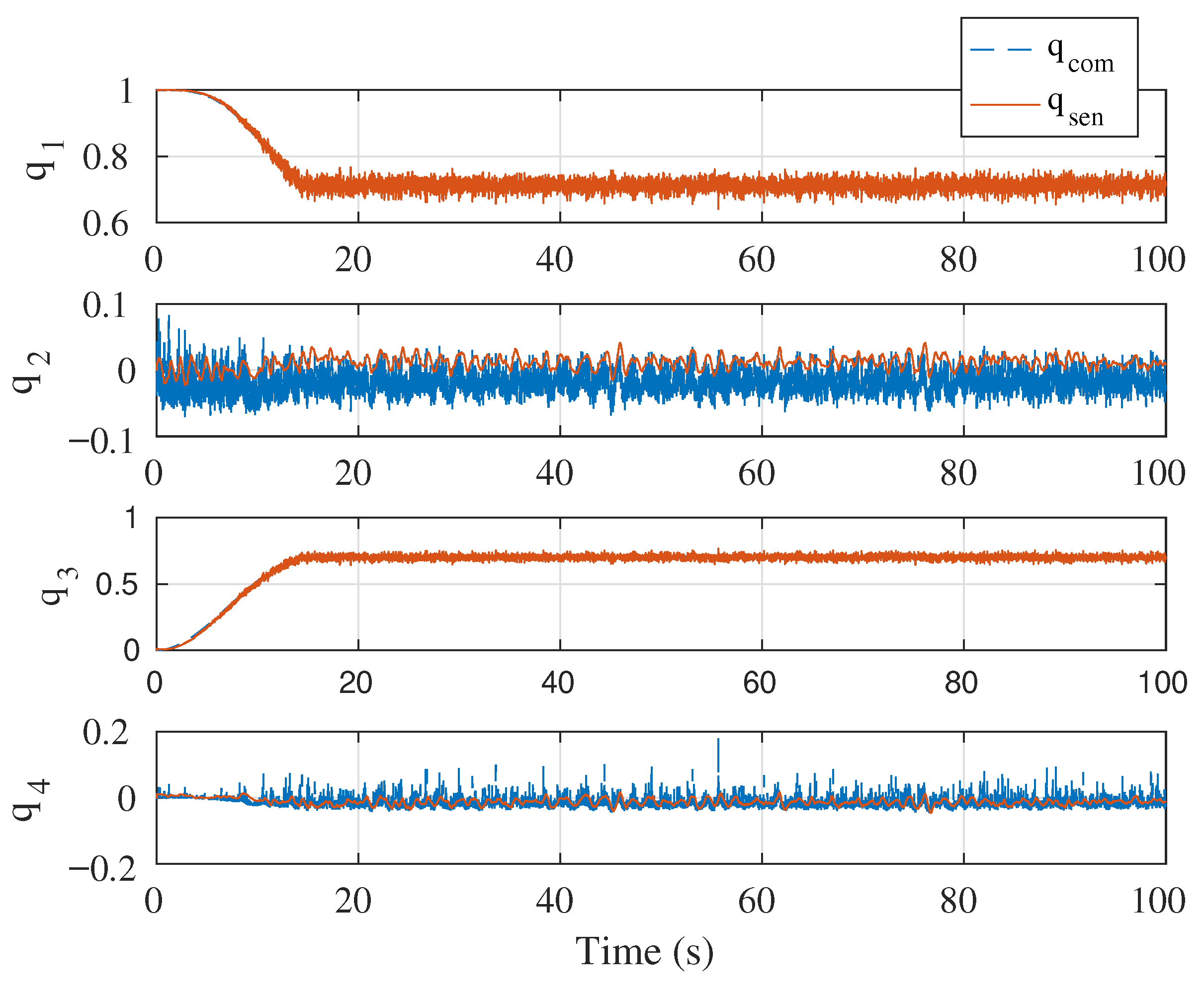
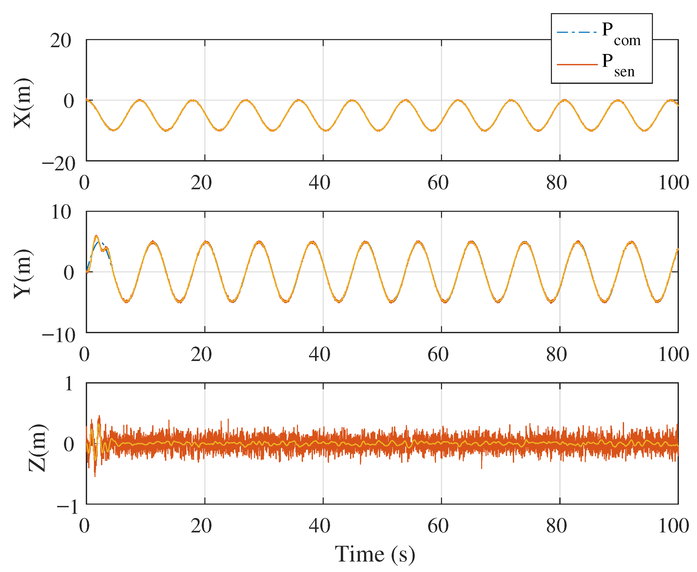
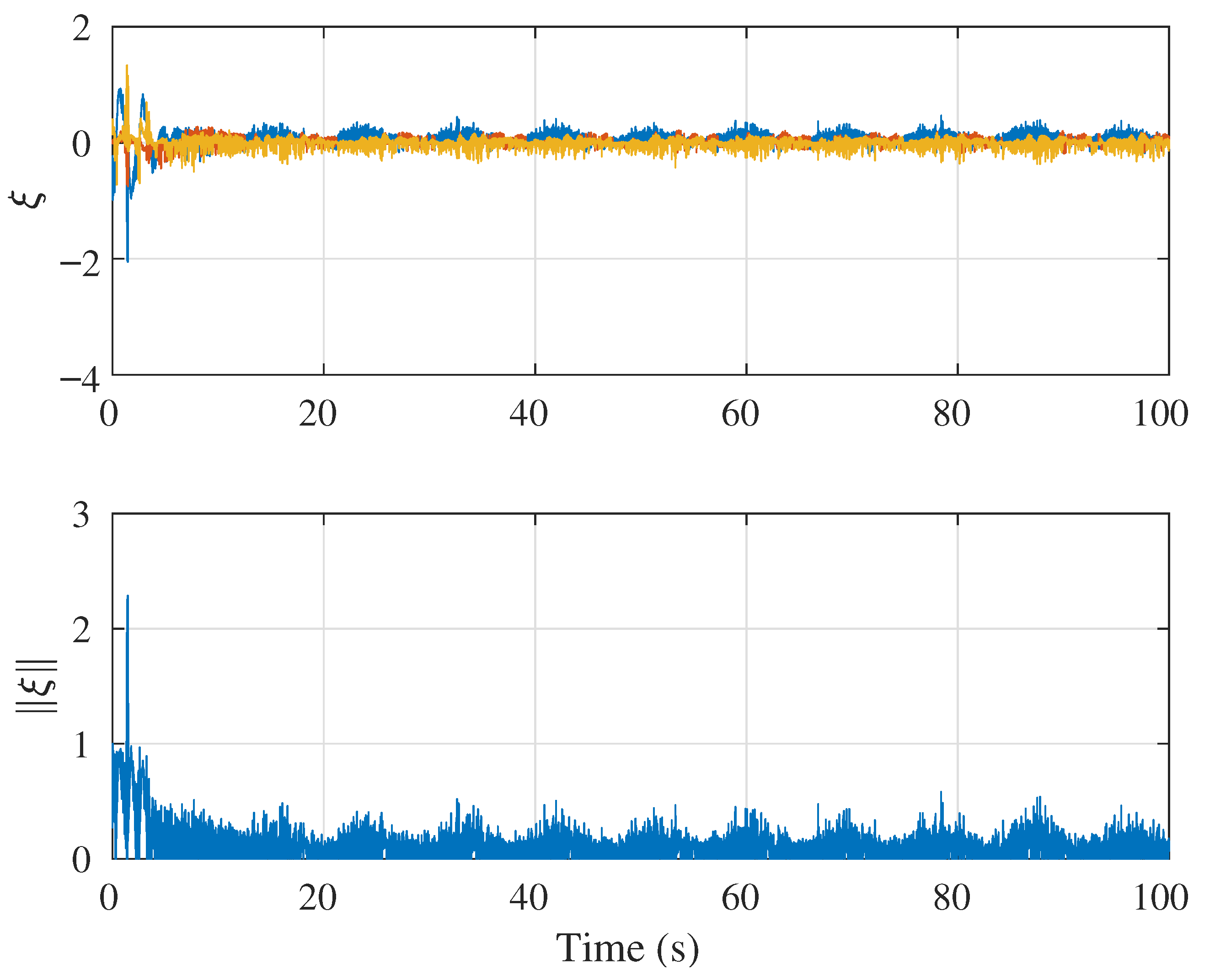
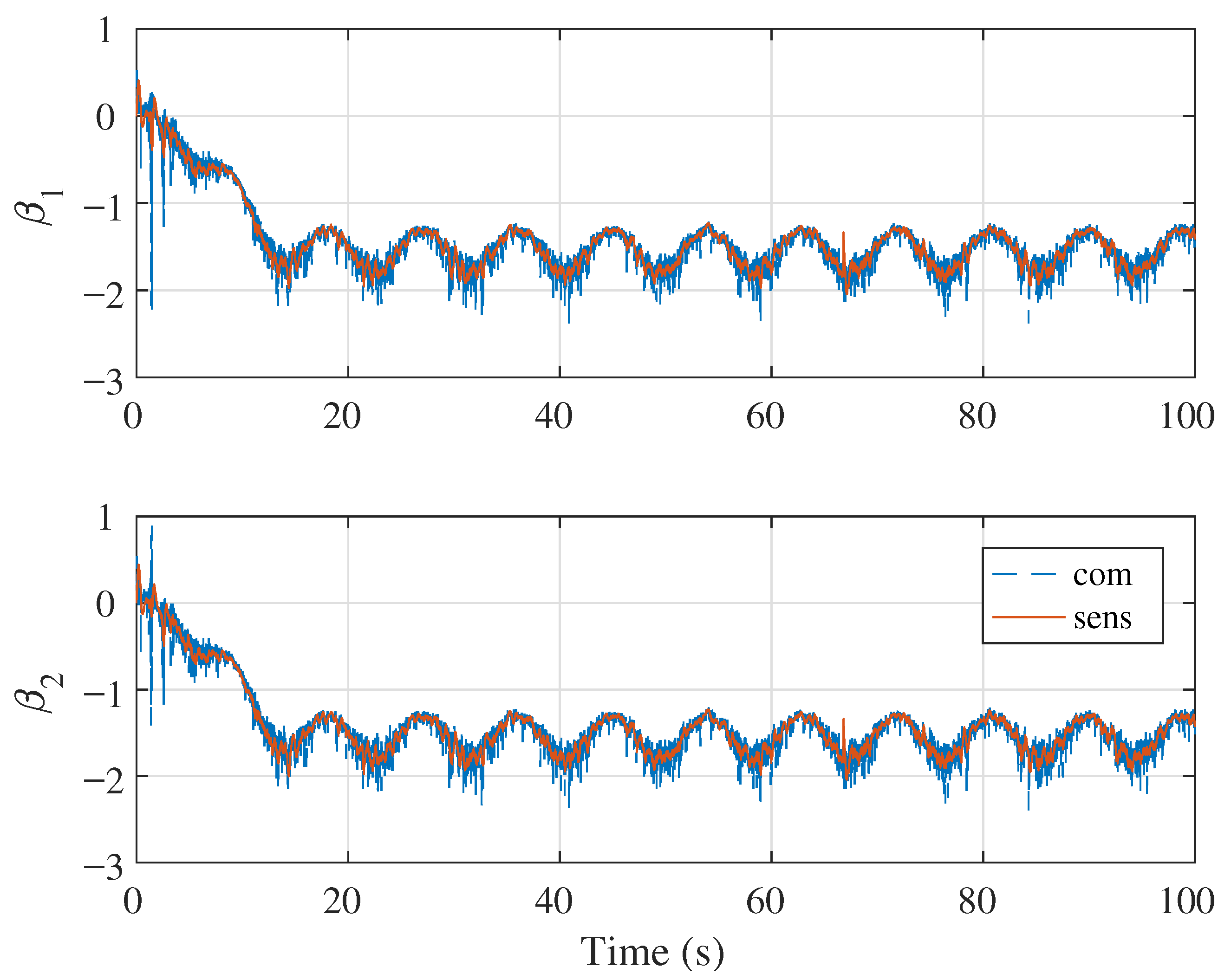
5.2. Simulation Case 2: Circular Position Tracking

We conducted another simulation in which the yaw and pitch angle commands remain the same as in the previous case, while the position commands vary over time. In this scenario, the position follows a circular trajectory, as shown in Figure 16 and Figure 17. The parameters, noise levels, and uncertainties are consistent with those of the previous simulation. The results, presented in Figure 17, Figure 18, Figure 19 and Figure 20, demonstrate that the PDUAV successfully tracks the time-varying position trajectory while adjusting its pitch angle. This capability is not achievable with a traditional quadrotor system. As shown in Figure 20, the joint angles follow sinusoidal trajectories to achieve the control objective.

6. Conclusions

This paper presents a singularity-free controller for the proposed PADUAV system, developed within the control framework of a class of 5-DOF aerial vehicles. A key component is the allocation module, which maps the output of the position controller to the desired attitude of the 5-DOF system. By introducing an intermediate reference frame, the controller is able to compute a valid reference attitude, even in singular configurations. To resolve the challenge of control allocation in these configurations, the two quadrotors are assigned different attitudes, effectively avoiding the secondary issue associated with singularity. The simulation results verify the controller’s ability to handle singular configurations and maintain system stability. The proposed controller extends the operational workspace of the aerial platform and improves its agility. Nonetheless, the current work is subject to certain limitations. The dynamics of the rotor-actuators were simplified and may not fully capture hardware behavior under high-frequency motion or disturbances. As future work, we plan to integrate motion planning strategies that are compatible with the singularity-free controller and validate the proposed approach through hardware-in-the-loop (HIL) simulations and real-world experiments using a physical prototype of the PADUAV platform.

References

1. Ding, X.; Guo, P.; Xu, K.; Yu, Y. A review of aerial manipulation of small-scale rotorcraft unmanned robotic systems. Chin. J. Aeronaut. 2019, 32, 200–214. [Google Scholar] [CrossRef]
2. Lippiello, V.; Fontanelli, G.A.; Ruggiero, F. Image-based visual-impedance control of a dual-arm aerial manipulator. IEEE Robot. Autom. Lett. 2018, 3, 1856–1863. [Google Scholar] [CrossRef]
3. Wang, M.; Chen, Z.; Guo, K.; Yu, X.; Zhang, Y.; Guo, L.; Wang, W. Millimeter-Level Pick and Peg-in-Hole Task Achieved by Aerial Manipulator. IEEE Trans. Robot. 2024, 40, 1242–1260. [Google Scholar] [CrossRef]
4. Yu, Y.; Ding, X. A Global Tracking Controller for Underactuated Aerial Vehicles: Design, Analysis, and Experimental Tests on Quadrotor. IEEE/ASME Trans. Mechatronics 2016, 21, 2499–2511. [Google Scholar] [CrossRef]
5. Ollero, A.; Tognon, M.; Suarez, A.; Lee, D.; Franchi, A. Past, Present, and Future of Aerial Robotic Manipulators. IEEE Trans. Robot. 2022, 38, 626–645. [Google Scholar] [CrossRef]
6. Kim, S.J.; Lee, D.Y.; Jung, G.P.; Cho, K.J. An origami-inspired, self-locking robotic arm that can be folded flat. Sci. Robot. 2018, 3, eaar2915. [Google Scholar] [CrossRef] [PubMed]
7. Estrada, M.A.; Mintchev, S.; Christensen, D.L.; Cutkosky, M.R.; Floreano, D. Forceful manipulation with micro air vehicles. Sci. Robot. 2018, 3, eaau6903. [Google Scholar] [CrossRef] [PubMed]
8. Ruggiero, F.; Lippiello, V.; Ollero, A. Aerial manipulation: A literature review. IEEE Robot. Autom. Lett. 2018, 3, 1957–1964. [Google Scholar] [CrossRef]
9. Meng, X.; He, Y.; Han, J. Survey on aerial manipulator: System, modeling, and control. Robotica 2020, 38, 1288–1317. [Google Scholar] [CrossRef]
10. Ryll, M.; Muscio, G.; Pierri, F.; Cataldi, E.; Antonelli, G.; Caccavale, F.; Bicego, D.; Franchi, A. 6D interaction control with aerial robots: The flying end-effector paradigm. Int. J. Robot. Res. 2019, 38, 1045–1062. [Google Scholar] [CrossRef]
11. Rajappa, S.; Ryll, M.; Bülthoff, H.H.; Franchi, A. Modeling, control and design optimization for a fully-actuated hexarotor aerial vehicle with tilted propellers. In Proceedings of the 2015 IEEE International Conference on Robotics and Automation (ICRA), Seattle, WA, USA, 26–30 May 2015; pp. 4006–4013. [Google Scholar] [CrossRef]
12. Brunner, M.; Rizzi, G.; Studiger, M.; Siegwart, R.; Tognon, M. A planning-and-control framework for aerial manipulation of articulated objects. IEEE Robot. Autom. Lett. 2022, 7, 10689–10696. [Google Scholar] [CrossRef]
13. Bodie, K.; Brunner, M.; Pantic, M.; Walser, S.; Pfändler, P.; Angst, U.; Siegwart, R.; Nieto, J. Active Interaction Force Control for Contact-Based Inspection With a Fully Actuated Aerial Vehicle. IEEE Trans. Robot. 2021, 37, 709–722. [Google Scholar] [CrossRef]
14. Park, S.; Lee, J.; Ahn, J.; Kim, M.; Her, J.; Yang, G.H.; Lee, D. ODAR: Aerial Manipulation Platform Enabling Omnidirectional Wrench Generation. IEEE/ASME Trans. Mechatronics 2018, 23, 1907–1918. [Google Scholar] [CrossRef]
15. Zheng, P.; Tan, X.; Kocer, B.B.; Yang, E.; Kovac, M. TiltDrone: A fully-actuated tilting quadrotor platform. IEEE Robot. Autom. Lett. 2020, 5, 6845–6852. [Google Scholar] [CrossRef]
16. Yiğit, A.; Perozo, M.A.; Cuvillon, L.; Durand, S.; Gangloff, J. Novel omnidirectional aerial manipulator with elastic suspension: Dynamic control and experimental performance assessment. IEEE Robot. Autom. Lett. 2021, 6, 612–619. [Google Scholar] [CrossRef]
17. Jiao, R.; Rong, Y.; Dong, M.; Li, J. Hybrid-disturbance-observer-based interaction control for a fully actuated UAV with tether-based positioning system. Ind. Robot. Int. J. Robot. Res. Appl. 2023, 50, 740–752. [Google Scholar] [CrossRef]
18. Shi, C.; Wang, K.; Yu, Y. Expandable Fully Actuated Aerial Vehicle Assembly: Geometric Control Adapted from an Existing Flight Controller and Real-World Prototype Implementation. Drones 2022, 6, 272. [Google Scholar] [CrossRef]
19. Du, J.; Wang, K.; Fan, Y.; Lai, G.; Yu, Y. High-Fidelity Integrated Aerial Platform Simulation for Control, Perception, and Learning. IEEE Trans. Autom. Sci. Eng. 2025, 22, 13662–13683. [Google Scholar] [CrossRef]
20. Lee, T. Geometric Control of Quadrotor UAVs Transporting a Cable-Suspended Rigid Body. IEEE Trans. Control Syst. Technol. 2018, 26, 255–264. [Google Scholar] [CrossRef]
21. Six, D.; Briot, S.; Chriette, A.; Martinet, P. The Kinematics, Dynamics and Control of a Flying Parallel Robot With Three Quadrotors. IEEE Robot. Autom. Lett. 2018, 3, 559–566. [Google Scholar] [CrossRef]
22. Cardona, G.; Tellez-Castro, D.; Mojica-Nava, E. Cooperative Transportation of a Cable-Suspended Load by Multiple Quadrotors. IFAC-PapersOnLine 2019, 52, 145–150. [Google Scholar] [CrossRef]
23. Nguyen, H.; Dang, T.; Alexis, K. The Reconfigurable Aerial Robotic Chain: Modeling and Control. In Proceedings of the 2020 IEEE International Conference on Robotics and Automation (ICRA), Paris, France, 31 May–31 August 2020; pp. 5328–5334. [Google Scholar] [CrossRef]
24. Nguyen, H.N.; Park, S.; Park, J.; Lee, D. A Novel Robotic Platform for Aerial Manipulation Using Quadrotors as Rotating Thrust Generators. IEEE Trans. Robot. 2018, 34, 353–369. [Google Scholar] [CrossRef]
25. Su, Y.; Jiao, Z.; Zhang, Z.; Zhang, J.; Li, H.; Wang, M.; Liu, H. Flight Structure Optimization of Modular Reconfigurable UAVs. In Proceedings of the 2024 IEEE/RSJ International Conference on Intelligent Robots and Systems (IROS), Abu Dhabi, United Arab Emirates, 14–18 October 2024; pp. 4556–4562. [Google Scholar] [CrossRef]
26. Su, Y.; Yu, P.; Gerber, M.J.; Ruan, L.; Tsao, T.C. Fault-Tolerant Control of an Overactuated UAV Platform Built on Quadcopters and Passive Hinges. IEEE/ASME Trans. Mechatronics 2024, 29, 602–613. [Google Scholar] [CrossRef]
27. Su, Y.; Zhang, J.; Jiao, Z.; Li, H.; Wang, M.; Liu, H. Real-time Dynamic-consistent Motion Planning for Over-actuated UAVs. In Proceedings of the 2024 IEEE International Conference on Robotics and Automation (ICRA), Yokohama, Japan, 13–17 May 2024; pp. 11789–11795. [Google Scholar] [CrossRef]
28. Ruan, L.; Pi, C.H.; Su, Y.; Yu, P.; Cheng, S.; Tsao, T.C. Control and experiments of a novel tiltable-rotor aerial platform comprising quadcopters and passive hinges. Mechatronics 2023, 89, 102927. [Google Scholar] [CrossRef]
29. Pereira, P.O.; Dimarogonas, D.V. Collaborative transportation of a bar by two aerial vehicles with attitude inner loop and experimental validation. In Proceedings of the 2017 IEEE 56th Annual Conference on Decision and Control (CDC), Melbourne, VIC, Australia, 12–15 December 2017; pp. 1815–1820. [Google Scholar]
30. Bosio, C.; Mueller, M.W. Automated Layout and Control Co-Design of Robust Multi-UAV Transportation Systems. IEEE Robot. Autom. Lett. 2025, 10, 3956–3963. [Google Scholar] [CrossRef]
31. Li, J.; Sugihara, J.; Zhao, M. Servo Integrated Nonlinear Model Predictive Control for Overactuated Tiltable-Quadrotors. IEEE Robot. Autom. Lett. 2024, 9, 8770–8777. [Google Scholar] [CrossRef]
32. Nishio, T.; Zhao, M. Singularity-Free Flight using Rotor-Distributed Aerial Manipulator. IEEE Robot. Autom. Lett. 2024, 9, 1460–1467. [Google Scholar] [CrossRef]
33. Nishio, T.; Zhao, M.; Okada, K.; Inaba, M. Design, Control, and Motion-Planning for a Root-Perching Rotor-Distributed Manipulator. IEEE Trans. Robot. 2023, 40, 660–676. [Google Scholar] [CrossRef]
34. Ding, C.; Lu, L. A Tilting-Rotor Unmanned Aerial Vehicle for Enhanced Aerial Locomotion and Manipulation Capabilities: Design, Control, and Applications. IEEE/ASME Trans. Mechatronics 2021, 26, 2237–2248. [Google Scholar] [CrossRef]
35. Ding, C.; Lu, L.; Wang, C.; Ding, C. Design, Sensing, and Control of a Novel UAV Platform for Aerial Drilling and Screwing. IEEE Robot. Autom. Lett. 2021, 6, 3176–3183. [Google Scholar] [CrossRef]
36. Qin, Z.; Wei, J.; Cao, M.; Chen, B.; Li, K.; Liu, K. Design and Flight Control of a Novel Tilt-Rotor Octocopter Using Passive Hinges. IEEE Robot. Autom. Lett. 2024, 9, 199–206. [Google Scholar] [CrossRef]
37. Yu, Y.; Lippiello, V. 6D Pose Task Trajectory Tracking for a Class of 3D Aerial Manipulator From Differential Flatness. IEEE Access 2019, 7, 52257–52265. [Google Scholar] [CrossRef]
38. Welde, J.; Kumar, V. Coordinate-free dynamics and differential flatness of a class of 6DOF aerial manipulators. In Proceedings of the 2020 IEEE International Conference on Robotics and Automation (ICRA), Paris, France, 31 May–31 August 2020; pp. 4307–4313. [Google Scholar]
39. Sun, J.; Wang, K.; Shi, C.; Li, X.; Yi, X.; Yu, Y.; Sun, F.; Dong, Y. Modeling and Control of PADUAV: A Passively Articulated Dual UAVs Platform for Aerial Manipulation*. In Proceedings of the 2024 IEEE International Conference on Robotics and Automation (ICRA), Yokohama, Japan, 13–17 May 2024; pp. 6159–6165. [Google Scholar] [CrossRef]
40. Van Nieuwstadt, M.J.; Murray, R.M. Real-time trajectory generation for differentially flat systems. Int. J. Robust Nonlinear Control 1998, 8, 995–1020. [Google Scholar] [CrossRef]
41. Iserles, A.; Munthe-Kaas, H.Z.; Norsett, S.P.; Zanna, A. Lie-group methods. Acta Numer. 2000, 9, 215–365. [Google Scholar] [CrossRef]
42. Murray, R.M.; Li, Z.; Sastry, S.S. A Mathematical Introduction to Robotic Manipulation; CRC Press, Inc.: Boca Raton, FL, USA, 1994. [Google Scholar]
43. Kendoul, F. Nonlinear Hierarchical Flight Controller for Unmanned Rotorcraft: Design, Stability, and Experiments. J. Guigance, Control. Dyn. 2009, 32, 1954–1958. [Google Scholar] [CrossRef]
44. Khalil, H.K.; Grizzle, J.W. Nonlinear Systems; Prentice Hall: Upper Saddle River, NJ, USA, 2002; Volume 3. [Google Scholar]
45. Wang, K.; Lai, G.; Yu, Y.; Du, J.; Sun, J.; Xu, B.; Franchi, A.; Sun, F. Versatile Tasks on Integrated Aerial Platforms Using Only Onboard Sensors: Control, Estimation, and Validation. IEEE Trans. Robot. 2025, 41, 3518–3538. [Google Scholar] [CrossRef]
46. Lee, D. Passive Decomposition and Control of Nonholonomic Mechanical Systems. IEEE Trans. Robot. 2010, 26, 978–992. [Google Scholar] [CrossRef]
47. Yang, H.; Lee, D. Dynamics and Control of Quadrotor with Robotic Manipulator. In Proceedings of the IEEE International Conference on Robotics and Automation (ICRA), Hong Kong, China, 31 May–7 June 2014; pp. 5544–5549. [Google Scholar]
Figure 1. Schematic of a class of 5-DOF aerial vehicles. The torque exerted on the vehicle is three-dimensional, while the force is confined to the body frame’s x - z plane, making it two-dimensional.
Drones 09 00503 g001
Figure 2. Prototype of the proposed PADUAV platform.
Drones 09 00503 g002
Figure 3. Since the articulated joints are passive, the PADUAV in this configuration cannot generate torque around the y axis of the body frame, nor can it generate force in a direction perpendicular to gravity.
Drones 09 00503 g003
Figure 4. The PADUAV travels across the vertical narrow space (left) with rotating valves on the wall (right). It cannot generate rotation torque when it reaches the vertical configuration, where one quadrotor is right above the other; thus, maintaining the system’s stability is a challenging problem.
Drones 09 00503 g004
Figure 5. Overall control architecture of a class of 5-DOF aerial vehicles. The system generates torque in three dimensions, while the controllable force is limited to a two-dimensional subspace.
Drones 09 00503 g005
Figure 6. Thrust and torques generated in the PADUAV.
Drones 09 00503 g006
Figure 7. Schematic diagram of the proposed control framework. It consists of the 5-DOF geometric tracking controller introduced in the previous section, along with a dedicated attitude control allocation module. The objective is to ensure that the position, yaw angle, and pitch angle track the desired trajectory. The position controller corresponds to the locked system controller, while the attitude controller and the joint position tracking controller correspond to the shape system controller.
Drones 09 00503 g007
Figure 8. Position tracking result in simulation case 1.
Drones 09 00503 g008
Figure 9. Attitude tracking result in Euler angles. Note that the apparent jump from π to π (or vice versa) in Euler angles is a representational artifact; both values correspond to the same physical orientation and do not indicate a real change in attitude.
Drones 09 00503 g009
Figure 10. Attitude tracking error in simulation case 1.
Drones 09 00503 g010
Figure 11. The attitude is shown using quaternions. It can be observed that there is no discontinuity in the attitude after the pitch angle reaches approximately π / 2 radians in simulation case 1.
Drones 09 00503 g011
Figure 16. The position trajectory is circular in case 2.
Drones 09 00503 g016
Figure 17. Position tracking result in simulation case 2. The position trajectory is circular.
Drones 09 00503 g017
Figure 18. The attitude is shown using quaternions in simulation case 2.
Drones 09 00503 g018
Figure 19. Attitude tracking error in simulation case 2.
Drones 09 00503 g019
Figure 20. Joint position tracking in simulation case 2.
Drones 09 00503 g020