An Efficient Downwelling Light Sensor Data Correction Model for UAV Multi-Spectral Image DOM Generation

Abstract

The downwelling light sensor (DLS) is the industry-standard solution for generating UAV-based digital orthophoto maps (DOMs). Current mainstream DLS correction methods primarily rely on angle compensation. However, due to the temporal mismatch between the DLS sampling intervals and the exposure times of multispectral cameras, as well as external disturbances such as strong wind gusts and abrupt changes in flight attitude, DLS data often become unreliable, particularly at UAV turning points. Building upon traditional angle compensation methods, this study proposes an improved correction approach—FIM-DC (Fitting and Interpolation Model-based Data Correction)—specifically designed for data collection under clear-sky conditions and stable atmospheric illumination, with the goal of significantly enhancing the accuracy of reflectance retrieval. The method addresses three key issues: (1) field tests conducted in the Qingpu region show that FIM-DC markedly reduces the standard deviation of reflectance at tie points across multiple spectral bands and flight sessions, with the most substantial reduction from 15.07% to 0.58%; (2) it effectively mitigates inconsistencies in reflectance within image mosaics caused by anomalous DLS readings, thereby improving the uniformity of DOMs; and (3) FIM-DC accurately corrects the spectral curves of six land cover types in anomalous images, making them consistent with those from non-anomalous images. In summary, this study demonstrates that integrating FIM-DC into DLS data correction workflows for UAV-based multispectral imagery significantly enhances reflectance calculation accuracy and provides a robust solution for improving image quality under stable illumination conditions.

1. Introduction

The downwelling light sensor (DLS) is a mainstream and effective device for ensuring accurate surface reflectance retrieval from rotary-wing UAV remote sensing data. The current mainstream solution involves mounting a DLS on top of the UAV to avoid propeller or fuselage obstructions, enabling unobstructed measurement of total radiance energy [1,2,3]. Modern DLS systems typically integrate an inertial measurement unit (IMU) to compensate for UAV attitude changes (roll/pitch/yaw) in real time, significantly improving radiometric measurement stability for short-duration missions (e.g., MicaSense’s DLS2, DJI’s D-RTK 2, etc.) [4,5,6]. However, during actual operations of rotary-wing UAVs, two primary factors may cause DLS data anomalies: attitude abnormalities and temporal misalignment between irradiance sensing and image capture [7,8,9]. First, both attitude adjustment and resistance to strong wind gusts are achieved by regulating the rotational speeds of the four motors, enabling flight maneuvers including hovering, rolling, pitching, yawing, and braking [10,11,12]. For instance, when strong wind gusts blow from the left, the UAV experiences rightward push causing right roll (right side tilting downward) [13,14]. Although the system generates a leftward restoring torque to level the UAV, strong wind gusts may still induce significant attitude abnormalities. [15,16]. During turning maneuvers, nearly all rotary-wing UAVs implement a braking strategy by ‘accelerating front rotors while decelerating rear rotors,’ which creates a pitch-up torque that raises the nose—this braking action induces noticeable fore-aft oscillations [17,18]. Secondly, taking the commonly used MicaSense DLS 2 and Parrot Sequoia DLS as examples, these downwelling light sensors typically employ silicon photodiode arrays as internal detectors and are equipped with integration time control functionality [19,20,21]. The output of each spectral channel represents the integrated average of incident radiant energy received within a short sampling window, thereby enabling near-instantaneous sensing of downwelling irradiance. Although DLS systems and multispectral cameras are generally configured for ‘synchronized triggering’, the sampling periods of both systems are not strictly aligned in time [22,23,24]. Specifically, the integration time of the DLS can range from several hundred microseconds to tens of milliseconds, whereas the camera exposure duration is typically limited to only a few milliseconds [25,26]. The subtle yet inherent timing discrepancy has minimal impact during stable flight. However, it becomes pronounced during UAV turning or rapid attitude changes, potentially causing mismatch between DLS-recorded irradiance and actual illumination conditions at image capture moment, thus introducing reflectance estimation errors [23].

Currently, researchers have developed multiple solutions to address the two primary causes of DLS data anomalies during rotary-wing UAV operations, with particular focus on attitude abnormalities. These approaches fall into two main categories: hardware optimization and data post-processing [27,28]. In terms of hardware optimization, improving the mounting configuration of the DLS is the most straightforward approach [29,30]. The prevailing method involves mounting the DLS on a gimbal system to ensure it consistently faces the zenith during flight, thereby enabling stable downwelling irradiance measurements. For example, Xie et al. developed an upward gimbal-mounted downwelling spectrometer system, which reduced the standard deviation of surface reflectance by 86.1% under cloudy conditions and achieved an average reduction of 59.6% across varying weather conditions [31]. Additionally, researchers have introduced the FGI Aerial Image Reference System (FGI AIRS), which employs optical leveling techniques to compensate for sensor tilt of up to 15° [32]. Experimental results have demonstrated that optical leveling offers substantial improvements in radiometric measurement accuracy [33,34,35]. In contrast, data post-processing methods provide a viable alternative without adding extra hardware weight [36,37,38]. A common approach involves using attitude data recorded by the Inertial Measurement Unit (IMU)—including roll, pitch, and yaw angles—to correct the directional deviation of radiometric values in the imagery, thereby compensating for DLS errors caused by UAV tilting [39]. Moreover, some researchers have constructed illumination models by integrating IMU attitude data, timestamps, and geolocation information to correct non-uniform irradiance distribution resulting from changes in sensor orientation, such as those characterized by the Bidirectional Reflectance Distribution Function (BRDF), effectively enhancing radiometric consistency [40,41,42]. Another more advanced method is Radiometric Block Adjustment (RBA), which integrates radiometric correction into the image block adjustment process, akin to bundle adjustment in photogrammetry but applied to radiometric values rather than geometric positions [43,44,45]. Multiple studies have shown that RBA significantly improves the radiometric uniformity and reflectance accuracy of UAV imagery, particularly under challenging illumination conditions such as rapidly changing solar angles during dawn, dusk, or cloud-induced shading. However, despite these improvements, both hardware optimization and data post-processing approaches still exhibit notable limitations. On one hand, hardware-based solutions impose stringent requirements on system compatibility and payload capacity, which restricts their application on small- to medium-sized rotary UAV platforms. On the other hand, IMU-based compensation and illumination modeling often rely on high-precision synchronization and complex parameter modeling, making them vulnerable to environmental perturbations and data drift, and their correction performance may degrade under rapidly fluctuating light conditions or severe attitude changes [39,46,47]. Furthermore, while RBA effectively enhances consistency across image blocks, it often lacks the sensitivity to detect and correct subtle local anomalies (such as abrupt DLS deviations at specific moments) within a single flight strip, thereby limiting its ability to address micro-scale radiometric errors. Therefore, in light of the deficiencies in existing methods for handling localized DLS anomalies, there is an urgent need to develop a simplified, robust, and practically implementable DLS data optimization strategy to further enhance the capability of UAV-based high-precision surface reflectance retrieval.

To address the aforementioned challenges, this study proposes a data correction method based on fitting and interpolation models (FIM-DC), specifically tailored for DLS data collected by rotary-wing UAVs under clear-sky conditions. Building upon UAV attitude compensation, the FIM-DC method first performs curve fitting on the data acquired from each individual UAV flight and defines an acceptable range using appropriate reference values. Outliers falling outside this range are corrected through interpolation between adjacent data points, thereby ensuring both the accuracy of the corrected values and the continuity of the time series. This study provides a practical and scalable solution for enhancing the radiometric consistency of UAV remote sensing products.

2. Methodology

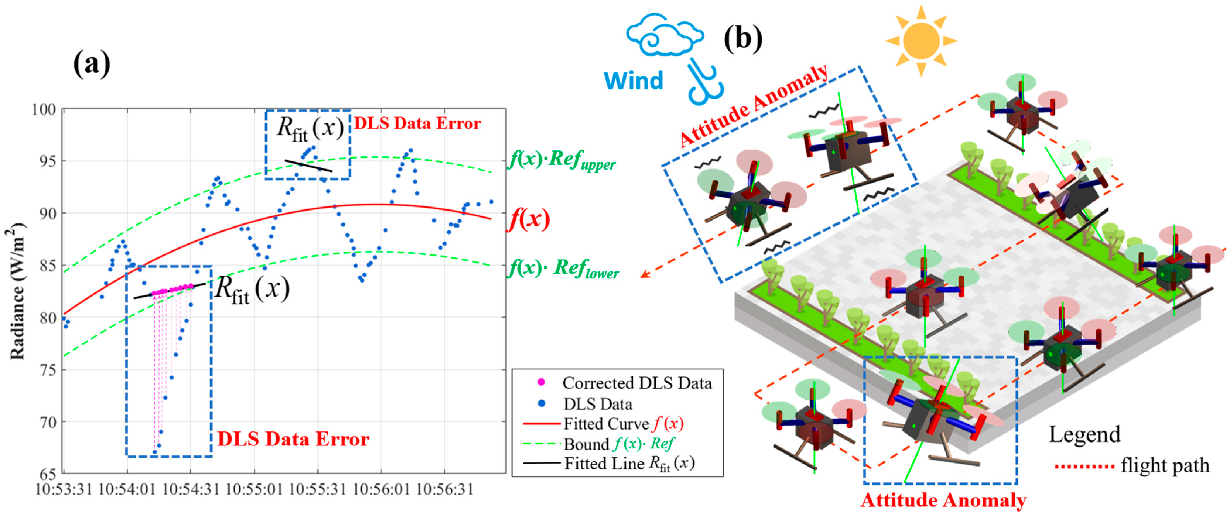
2.1. Construction of FIM-DC

The commonly adopted method for calculating reflectance using multispectral cameras involves installing an integrated DLS on top of the UAV prior to takeoff, which records real-time incident irradiance after attitude compensation by the IMU, as expressed in Equation (1). However, during route turning, nearly all rotary-wing UAVs employ a braking strategy that generates a pitching-up torque to lift the UAV’s nose and decelerate, as illustrated in Figure 1b. This maneuver leads to periodic oscillations in the DLS data recorded during a single flight mission and is one of the most common causes of DLS data instability, as shown by the orange dashed line in Figure 1a. In addition to this, other factors such as strong wind gusts may also introduce discontinuous anomalies into the DLS data, resembling the red dashed line in Figure 1a. To resolve this issue, the FIM-DC method introduces DLS data cleaning. In this mechanism, outlier points that fall beyond the ideal range are discarded and replaced with interpolated values between adjacent acceptable data points using linear fitting, as defined in Equation (2).

$$\mathrm{Traditional}:{\rho }_{\mathrm{image}}={\displaystyle \frac{R_{\mathrm{image}}\left(reflection\right)}{R_{\mathrm{DLS}}}}$$

(1)

$$\mathrm{FIM-DC}:{\rho }_{\mathrm{image}}={\displaystyle \frac{R_{\mathrm{image}}\left(reflection\right)}{{\widehat{R}}_{\text{DLS-cleaned}}}}=\left\{\begin{array}{l}{\displaystyle \frac{R_{\mathrm{image}}\left(reflection\right)}{R_{\mathrm{DLS}}}},R_{\mathrm{DLS}}\in \left[f(x)\cdot Re{f}_{upper},f(x)\cdot Re{f}_{lower}\right]\\ {\displaystyle \frac{R_{\mathrm{image}}\left(reflection\right)}{R_{\mathrm{fit}}(x)}},R_{\mathrm{DLS}}\notin \left[f(x)\cdot Re{f}_{upper},f(x)\cdot Re{f}_{lower}\right]\end{array}\right.$$

(2)

where ${\rho }_{\mathrm{image}}$ denotes the reflectance of the ground feature, and $R_{\mathrm{image}}\left(reflection\right)$ represents the reflected radiance energy. $R_{\mathrm{DLS}}$ and ${\widehat{R}}_{\text{DLS-cleaned}}$ correspond to the DLS-recorded incident radiance energy before and after correction, respectively. Curve $f(x)$ (the red curve in Figure 1a) represents the quadratic fitting of the original DLS data. The reference values $Re{f}_{upper}$ and $Re{f}_{lower}$ are critical correction parameters, which are determined autonomously through a comprehensive consideration of flight time, takeoff time, the oscillation range of the DLS data, and other relevant factors.

Based on $f(x)$ and the reference values $Re{f}_{upper}$ and $Re{f}_{lower}$, the range requiring correction can be identified, as indicated by the two green dashed lines in Figure 1a. For DLS data points falling within the range requiring correction, the FIM-DC method selects the two nearest neighboring points—located immediately before and after the sequence of continuous outliers—that fall outside the correction range, and performs a linear fitting based on these valid points. The resulting fitted line, denoted as line $R_{\mathrm{fit}}(x)$ (the black line in Figure 1a), is then used to compute the corrected DLS data (the purple data points in Figure 1a). Assuming the coordinates of the two nearest valid points are $({\mathrm{Time}}_1,R_{{\mathrm{DLS}}_1})$ and $({\mathrm{Time}}_2,R_{{\mathrm{DLS}}_2})$, the mathematical expression of line A is provided in Equation (3).

$$R_{\mathrm{fit}}(x)={\displaystyle \frac{R_{{\mathrm{DLS}}_2}-R_{{\mathrm{DLS}}_1}}{{\mathrm{Time}}_2-{\mathrm{Time}}_1}}(x-{\mathrm{Time}}_1)+R_{{\mathrm{DLS}}_1}$$

(3)

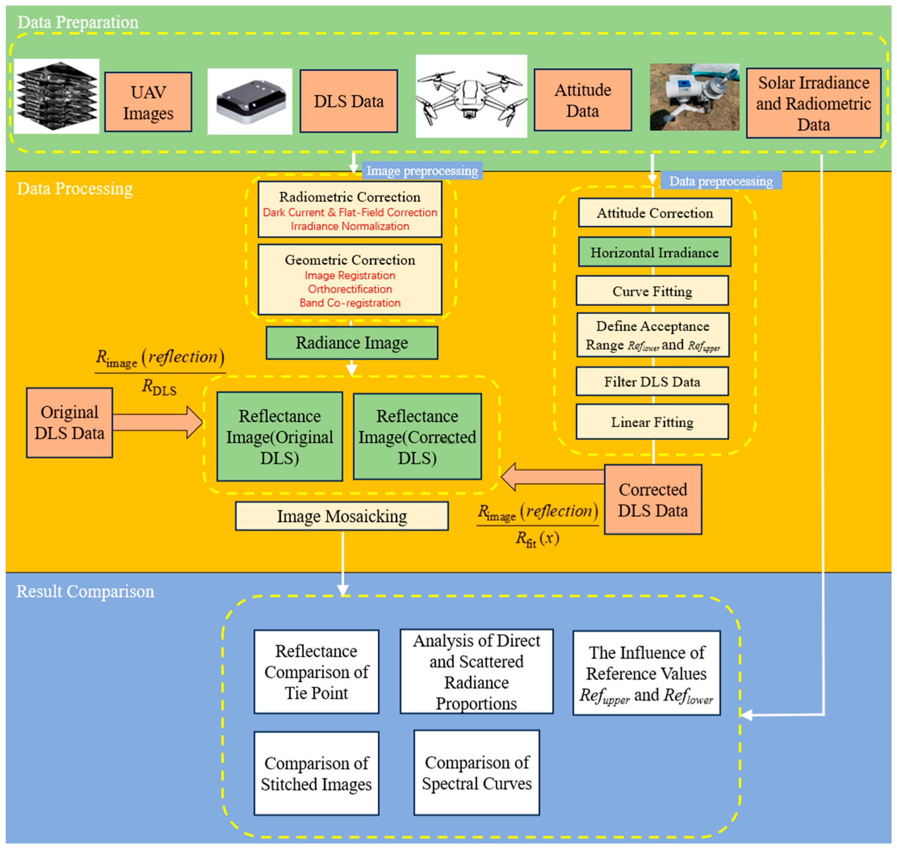
2.2. Experimental Procedure

The experiment comprised three main components: Data Preparation, Data Processing, and Result Comparison (as shown in Figure 2). In the Data Preparation phase, four types of data were collected: UAV Images, DLS Data, Attitude Data, and Solar Irradiance and Radiometric Data. Subsequently, image preprocessing was performed on the UAV imagery, including radiometric correction and geometric correction, resulting in the generation of radiance images. The radiometric correction process comprised two main steps. The first step was Dark Current and Flat-Field Correction, which aimed to eliminate the camera’s internal thermal noise and correct for illumination non-uniformity. The second step was Irradiance Normalization, which was necessary for the subsequent reflectance calculation. Geometric correction involved three components: image registration, orthorectification, and band co-registration. Next, the DLS Data were combined with the Attitude Data to perform Attitude Correction, thereby producing Horizontal Irradiance data (in some cases, DLS systems can directly provide Horizontal Irradiance). The proposed FIM-DC Model was then applied. First, Curve Fitting was conducted on the Horizontal Irradiance data. An Acceptance Range was defined using two reference values, $Re{f}_{upper}$ and $Re{f}_{lower}$. Following this, DLS Data Filtering was performed to remove outlier points that fell outside the acceptable range, and these removed points were subsequently supplemented using Linear Interpolation between adjacent valid data points. Based on this process, Reflectance Images were calculated using two methods: one based on the original DLS data (Reflectance Image (Original DLS)), and the other using the corrected DLS data (Reflectance Image (Corrected DLS)). These images were then used to perform Image Mosaicking, which served as the basis for subsequent result comparisons. In the Result Comparison phase, five aspects were analyzed: Reflectance Comparison of Tie Points, where tie points from images taken at different times were selected for comparison; analysis of the differences between Direct and Scattered Irradiance in DLS data and Solar Irradiance and Radiometric Data; Comparison of Stitched Images; Comparison of Spectral Curves; and finally, a discussion of the influence of the reference values $Re{f}_{upper}$ and $Re{f}_{lower}$ in the Section 5.3.

3. Experiments

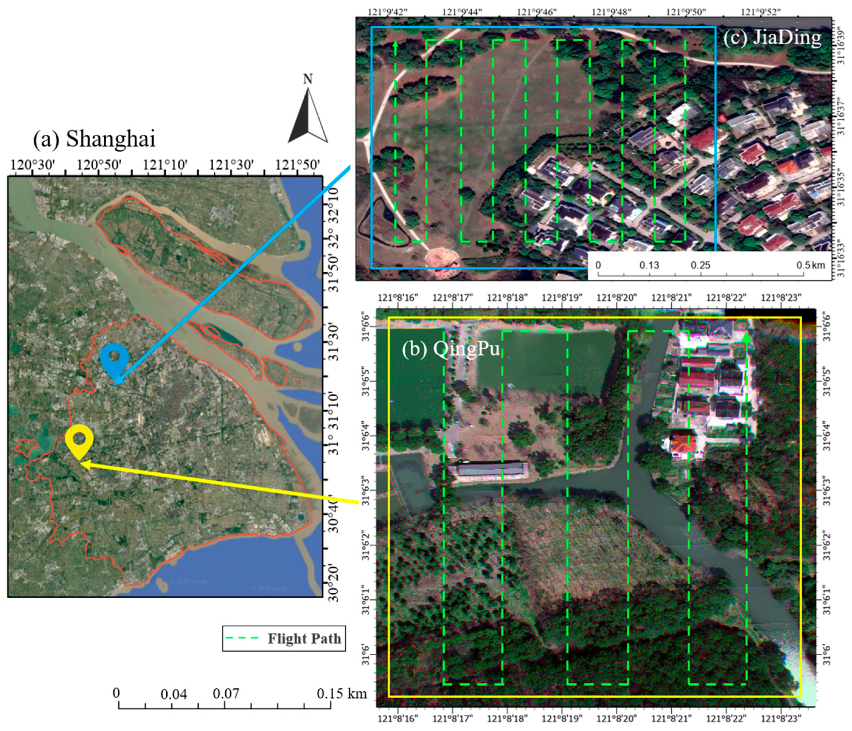
3.1. Experimental Design

The experiment was conducted in Qingpu District and Jiading District of Shanghai, China, with the central coordinates of the test areas located at [121°8′20″ E, 31°6′3″ N] and [121°9′47″ E, 31°16′36″ N] (see Figure 3). The tests were carried out on 18 March 2025, and 14 December 2023. The experimental area in Qingpu District covered approximately 8.6 ha, while the experimental area in Jiading District was 14 ha. Both experimental areas included diverse land cover types such as water bodies, artificial structures, trees, grassland, and bare soil. This research adopted 0.95 and 1.05 as the reference values. A rotary-wing UAV (DJI M300) equipped with a DLS was used to perform aerial photography missions. The UAV conducted flights approximately every 15 min, with each flight lasting about 15 min. The UAV flight path is indicated by the green dashed lines in Figure 3.

There were a total of five flight missions conducted in the Qingpu experiment. The takeoff times and landing times for each mission were 09:35:14, 10:45:31, 11:38:20, 13:02:56, and 14:47:44 for takeoff, and 09:52:05, 10:59:53, 11:49:20, 13:18:23, and 14:59:19 for landing, respectively. The flight parameters were configured with an 85% overlap rate, an 80% sidelap rate, and a flight altitude of 120 m. Detailed flight parameters are provided in

Table 1. UAV experimental operational parameters.

Parameter	QingPu Experiment	JiaDing Experiment
Area (ha)	8.6	14
Flight Overlap Rate (%)	85	85
Sidelap Rate (%)	80	80
Flight Altitude (m)	110	110

. Additionally, a solar radiometer and a solar direct irradiance radiometer were deployed on the ground to facilitate subsequent comparisons between DLS data and actual solar radiation energy measurements.

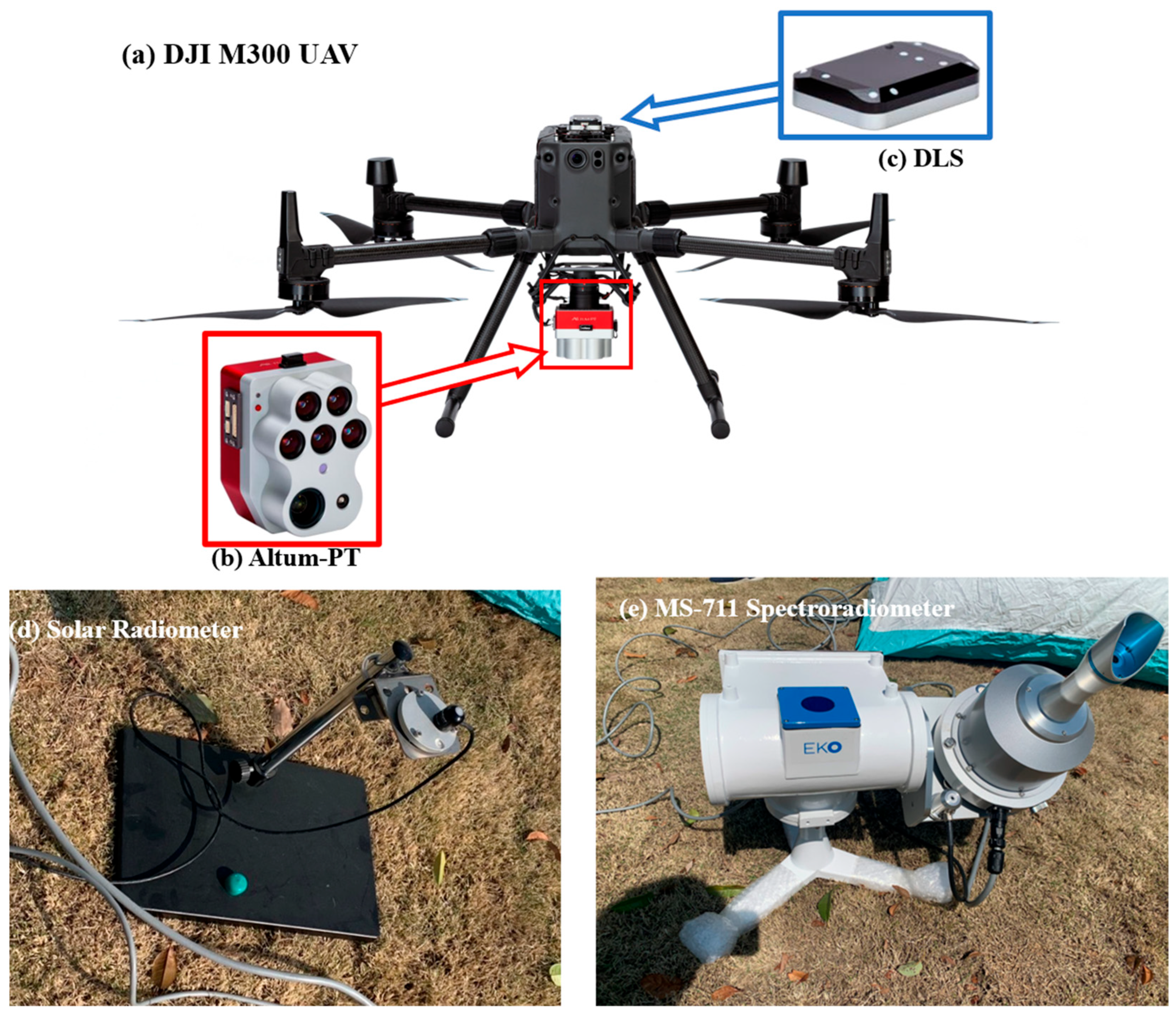
3.2. Experimental Equipment

The UAV used in this experiment was the DJI M300 rotary-wing UAV (SZ DJI Technology Co., Ltd., Shenzhen, Guangdong, China) (Figure 4a). The DJI M300 has a single flight time of 20–30 min. The payload equipped on the UAV was the Altum-PT multispectral camera (MicaSense, Inc., Rochester, MN, USA) (Figure 4b), with specific camera parameters provided in

Table 2. Detailed device characteristics.

MS-711 Spectroradiometer	Main Parameters
Wavelength Range	300–1100 nm
Optical Resolution (FWHM)	<7 nm
Wavelength Accuracy	±0.2 nm
Cosine Response (0–80°)	<5%
Exposure Time	10 ms to 5 s
Field of View (FOV)	180°
Dimensions and Weight	220 mm × 197 mm, approximately 4.5 kg
Altum-pt multispectral camera	Main parameters
Field of View	46° HFOV × 35° VFOV
Ground Resolution	5.28 cm perpixel at 120 m
Image Resolution	2064 × 1544
Blue band	475 ± 32 nm
Green band	560 ± 27 nm
Red band	668 ± 14 nm
Red Edge	717 ± 12 nm
Near-Infrared (NIR)	842 ± 57 nm
Panchromatic	634.5 ± 463 nm

. Additionally, the UAV was also equipped with the MicaSense DLS (MicaSense, Inc., Seattle, WA, USA) (Figure 4c), which weighs approximately 49g and has the same spectral bands as the Altum-PT camera. The DLS has a field of view of 180° and integrates a GPS system. Furthermore, in the ground-based experimental equipment, an MS-711 Spectroradiometer from EKO Instruments Co., Ltd. (Osaka, Japan) (Figure 4e) was installed. This is a solar direct irradiance radiometer that accurately records direct solar radiation energy, with spectral parameters and resolution that fully cover the spectral bands of the high-resolution camera. Detailed parameters are provided in Table 2. Additionally, a solar radiometer (Apogee Instruments, Inc., Logan, UT, USA) was used to record total solar radiation (Figure 4d). With the use of these two devices (solar radiometer and solar direct irradiance radiometer), the scattered radiation energy can be calculated.

4. Results

Four comparison approaches were employed to verify the effectiveness of the FIM-DC model. First, adjacent images were compared, with a focus on two spectral bands—the blue band and the red-edge band—captured at different flight times, to enhance data diversity and robustness. Second, the proportions of direct and scattered irradiance recorded by the DLS were visually compared with actual values, especially during UAV attitude anomalies. Third, stitched images generated from original and corrected datasets were compared to assess the impact of individual image corrections on overall mosaic quality. Additionally, spectral curves of multiple typical land cover types were analyzed across all multispectral bands to better reflect practical field applications. Finally, the influence of different parameter settings on model performance was evaluated using datasets from two experimental areas and two flight campaigns.

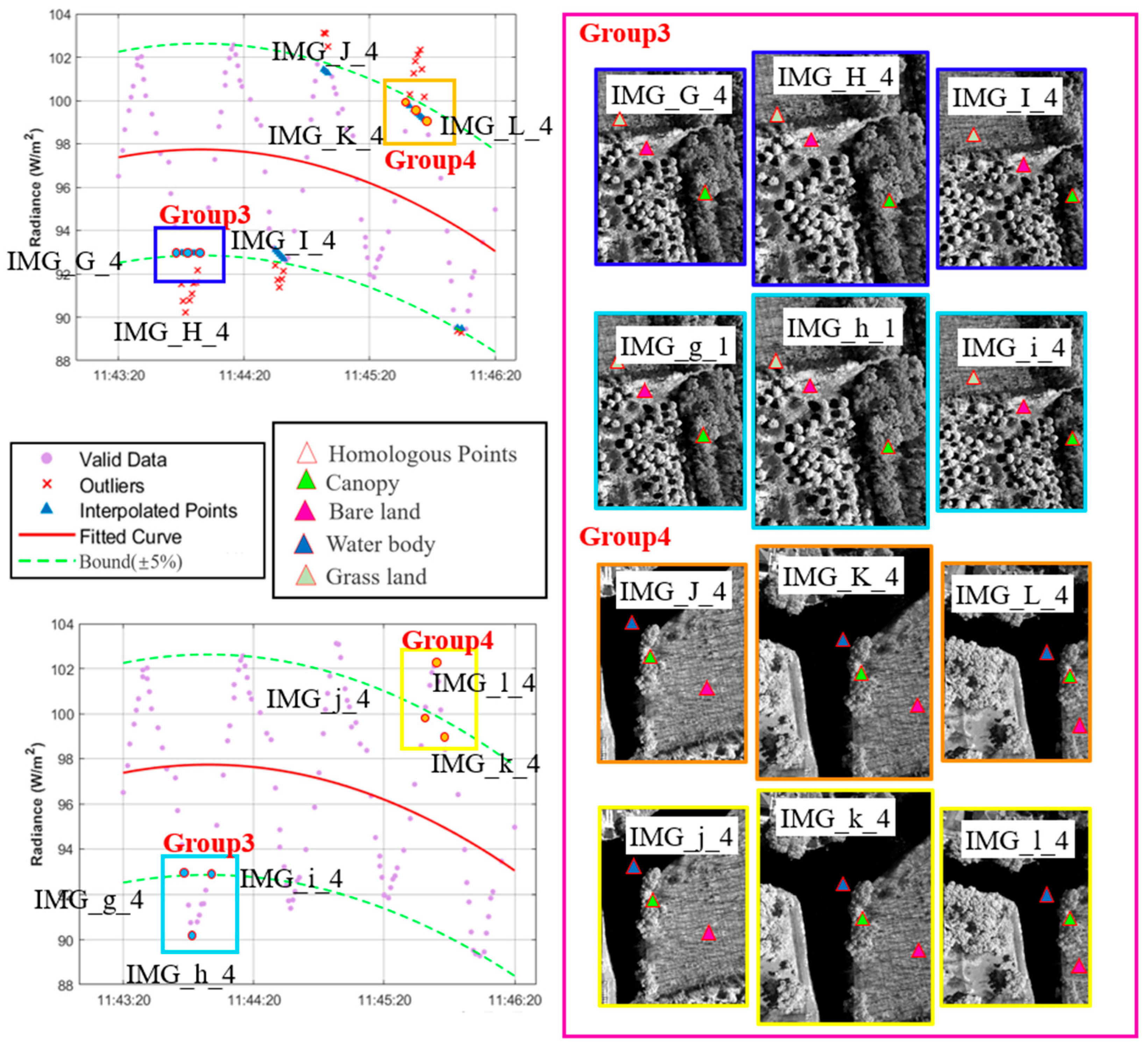
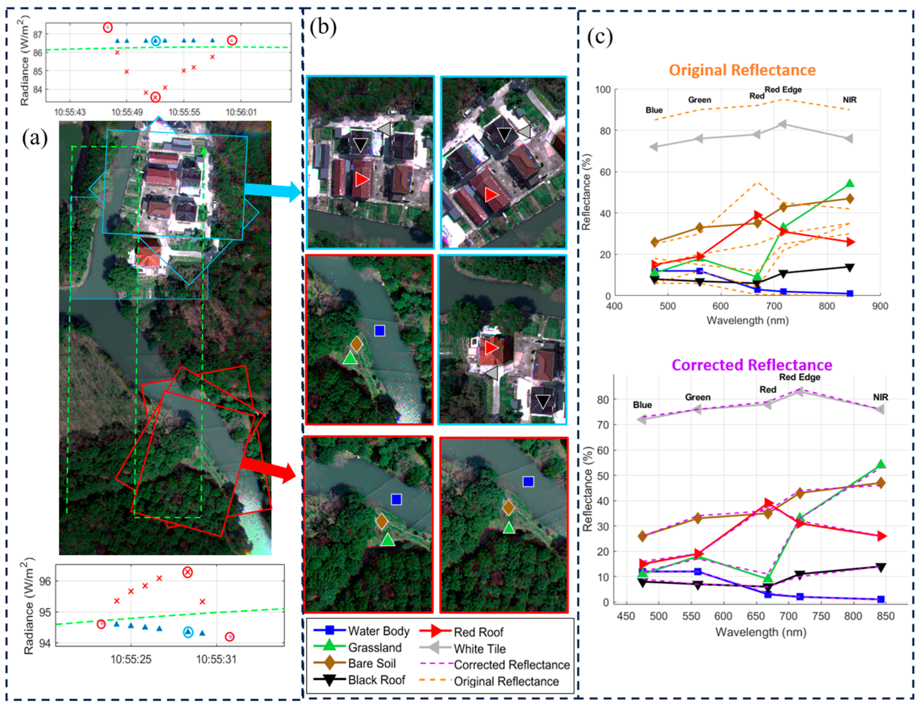
4.1. Tie Point Reflectance Comparison Between Adjacent Images

Tie points, which are points commonly captured across successive UAV images, should exhibit nearly identical reflectance values across all bands for the preceding and following five images. Therefore, when UAV attitude anomalies occur, the reflectance of tie points in the anomalous images deviates from that of the adjacent images. Consequently, whether the FIM-DC method can correct the reflectance values of tie points affected by attitude anomalies to match those in adjacent images serves as a crucial criterion for evaluating the effectiveness of FIM-DC. Figure 5 presents the data from the second flight mission of the Qingpu experiment, with a takeoff time of 10:45:31 and a landing time of 10:59:53. Tie points were selected for comparison from two groups: Group 1, in which the DLS data exhibited both positive and negative deviations, and Group 2, in which the DLS data showed consistently positive deviations. A total of four typical land cover types were selected from 12 images, namely canopy, bare land, water body, and cement road. As indicated in the figure captions of Figure 5, labels with uppercase letters (e.g., IMG_A_1) represent corrected data, while labels with lowercase letters (e.g., IMG_a_1) represent original, uncorrected data. Group 1 and Group 2 in Figure 5, respectively, illustrate the locations and types of the selected tie points.

Table 3. Reflectance of four land cover types across all images in Band 1.

Group 1
	Canopy	Bare Land
IMG_A_1	13%	32%
IMG_B_1	13%	31%
IMG_C_1	14%	32%
IMG_a_1	13%	32%
IMG_b_1	43%	62%
IMG_c_1	35%	51%
Group 2
	Canopy	Water body	Cement road
IMG_D_1	15%	5%	45%
IMG_E_1	15%	6%	45%
IMG_F_1	14%	6%	45%
IMG_d_1	15%	5%	45%
IMG_e_1	11%	2%	37%
IMG_f_1	14%	6%	45%

presents the reflectance comparison of the tie points shown in Figure 5. It can be observed that, after FIM-DC correction, the canopy reflectance in IMG_A_1, IMG_B_1, and IMG_C_1 remained stable at approximately 13%. In contrast, in the original uncorrected data (IMG_b_1 and IMG_c_1), the canopy reflectance surged to around 40% due to anomalies in the DLS data. The standard deviation was used to evaluate the degree of deviation in the data. Based on this, the standard deviation of canopy reflectance in Group 1 was calculated to be 15.07% before correction and reduced to 0.58% after applying the FIM-DC method.

Figure 6 presents the data from the third flight mission of the Qingpu experiment, with the takeoff time at 11:38:20 and the landing time at 11:49:20. To demonstrate the effectiveness of the FIM-DC method across different spectral bands, both Group 3 and Group 4 selected data from the red-edge band for comparison. Similarly to the previous analysis,

Table 4. Reflectance of four land cover types across all images in Band 4.

Group 3
	Canopy	Bare Land	Grass Land
IMG_A_4	33%	29%	45%
IMG_B_4	33%	29%	47%
IMG_C_4	32%	28%	46%
IMG_a_4	33%	29%	45%
IMG_b_4	45%	36%	52%
IMG_C_4	32%	28%	46%
Group 4
	Canopy	Water body	Bare land
IMG_D_4	35%	5%	35%
IMG_E_4	35%	4%	34%
IMG_F_4	37%	4%	33%
IMG_d_4	35%	5%	35%
IMG_e_4	26%	2%	24%
IMG_f_4	37%	4%	33%

shows the reflectance comparison of four types of land cover before and after FIM-DC correction, where IMG_D_1, IMG_E_1, and IMG_F_1 represent the corrected images, and IMG_d_1, IMG_e_1, and IMG_f_1 represent the original uncorrected images.

Combining the information from Figure 6 and Table 4, it can be observed that during the capture of IMG_b_1, the DLS data experienced a significant drop, resulting in a noticeably higher reflectance in IMG_b_1 compared to the adjacent images, as shown in Table 4. In contrast, for Group 4, the DLS data for IMG_e_1 was significantly elevated, causing its reflectance to be markedly lower than that of the preceding and succeeding images. These findings indirectly highlight the critical role of DLS data stability in the calculation of UAV reflectance and further demonstrate the effectiveness of the FIM-DC method.

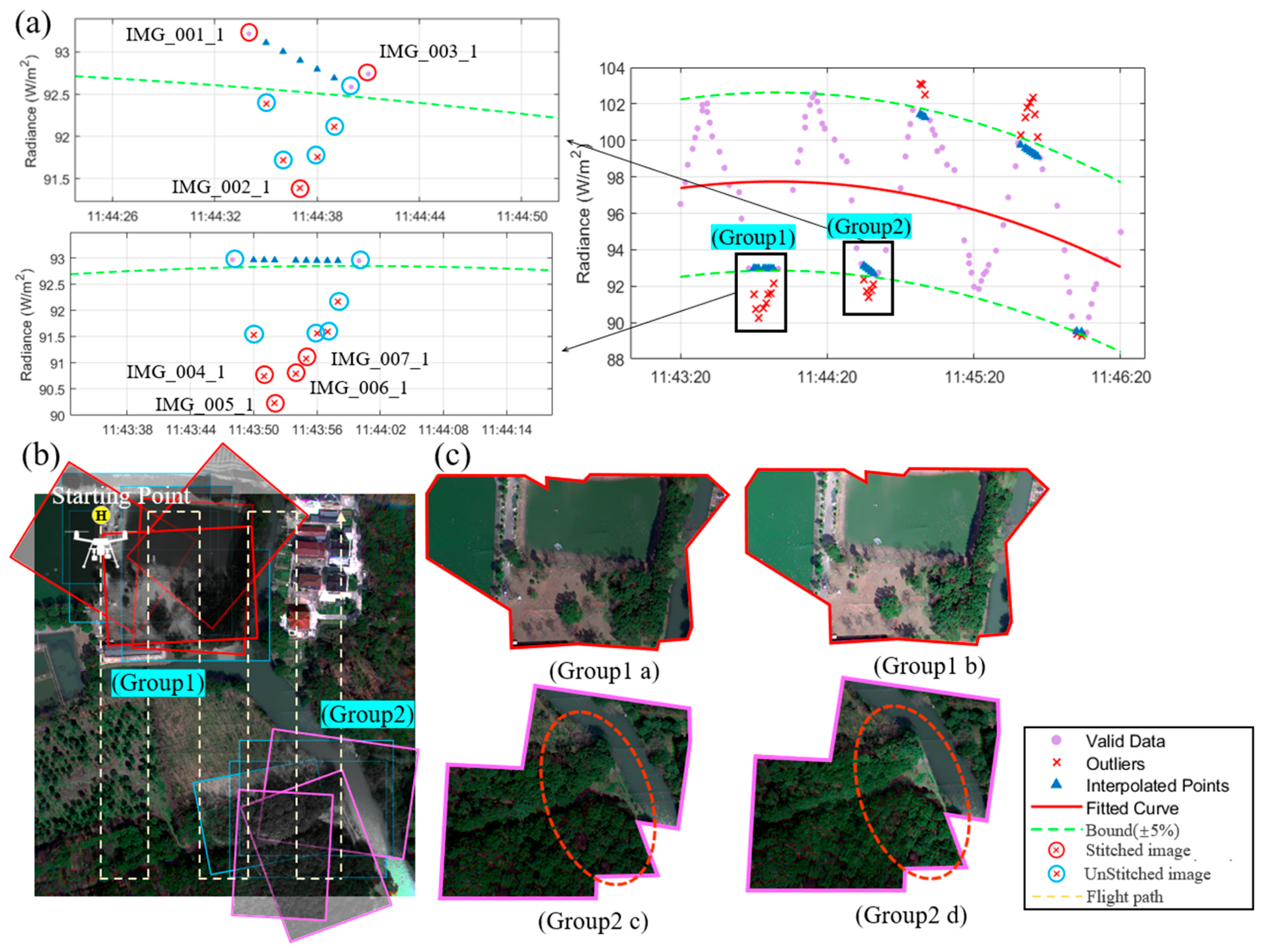
4.2. Comparison of Stitched Images

Stitched images provide a more intuitive way to observe the impact of DLS data anomalies on imagery quality. Figure 7 illustrates the results of stitching images before and after correction at the ends of two UAV flight strips.

Figure 7a shows the selected images for stitching: three images for Group 1 (IMG_001_1, IMG_002_1, IMG_003_1) and four images for Group 2 (IMG_004_1, IMG_005_1, IMG_006_1, IMG_007_1). Figure 7b displays their specific locations along the UAV flight path during a single mission, where all images are located near the turning points of the flight lines, thereby emphasizing the effect of “turning maneuvers” on DLS data stability. Figure 7c presents the stitched results. The two different selection strategies allow for a more comprehensive comparison. Group 1 selected three consecutive images, enabling an overall assessment of consistency, whereas Group 2 selected two images within the acceptable range and one outside the acceptable range, thereby simulating a more realistic stitching scenario. The results indicate that Group 1b is noticeably brighter overall than Group 1a, suggesting unreasonable reflectance values. Similarly, within Group 2, the regions enclosed by the red dashed lines in Group 2d and Group 2c exhibit inconsistencies in reflectance, primarily caused by the inclusion of an image outside the acceptable range. Group 1a and Group 2c, both corrected using the FIM-DC method, show more reasonable and consistent reflectance compared to their respective counterparts, further demonstrating the effectiveness of the FIM-DC method.

5. Discussion

5.1. Comparison of Spectral Curves of Tie Points

The spectral curves of tie points provide a reliable reference for assessing whether images with attitude anomalies have been properly corrected. To illustrate this, we selected two images within the acceptable range and one outside it for comparison, all located at turning points along the UAV flight path, as shown in Figure 8a. Six types of tie points were chosen for spectral curve comparison, including Water Body, Red Roof, Grassland, White Tile, Bare Soil, and Black Roof. These land cover types effectively demonstrate the performance of the FIM-DC model across different spectral regions. The specific locations of the tie points are shown in Figure 8b. Figure 8c presents the original and corrected spectral curves.

Figure 8c illustrates the original and corrected spectral curves. The spectral curves of the six land cover types were derived by calculating the reflectance from two images within the acceptable range. Figure 8c clearly demonstrates the effectiveness of the FIM-DC model in correcting UAV image reflectance. Overall, the corrected reflectance (represented by the purple dashed line) is significantly closer to the true land surface reflectance, whereas the original reflectance (orange dashed line) deviates considerably. This discrepancy in the original reflectance is primarily caused by abnormal UAV attitudes that result in erroneous DLS data. Specifically, for Red Roof and White Tile, the original reflectance shows a large deviation—approximately 15% in the 600–700 nm range—compared to the actual land surface reflectance, which is almost completely eliminated after correction with the FIM-DC model, highlighting the model’s effectiveness.

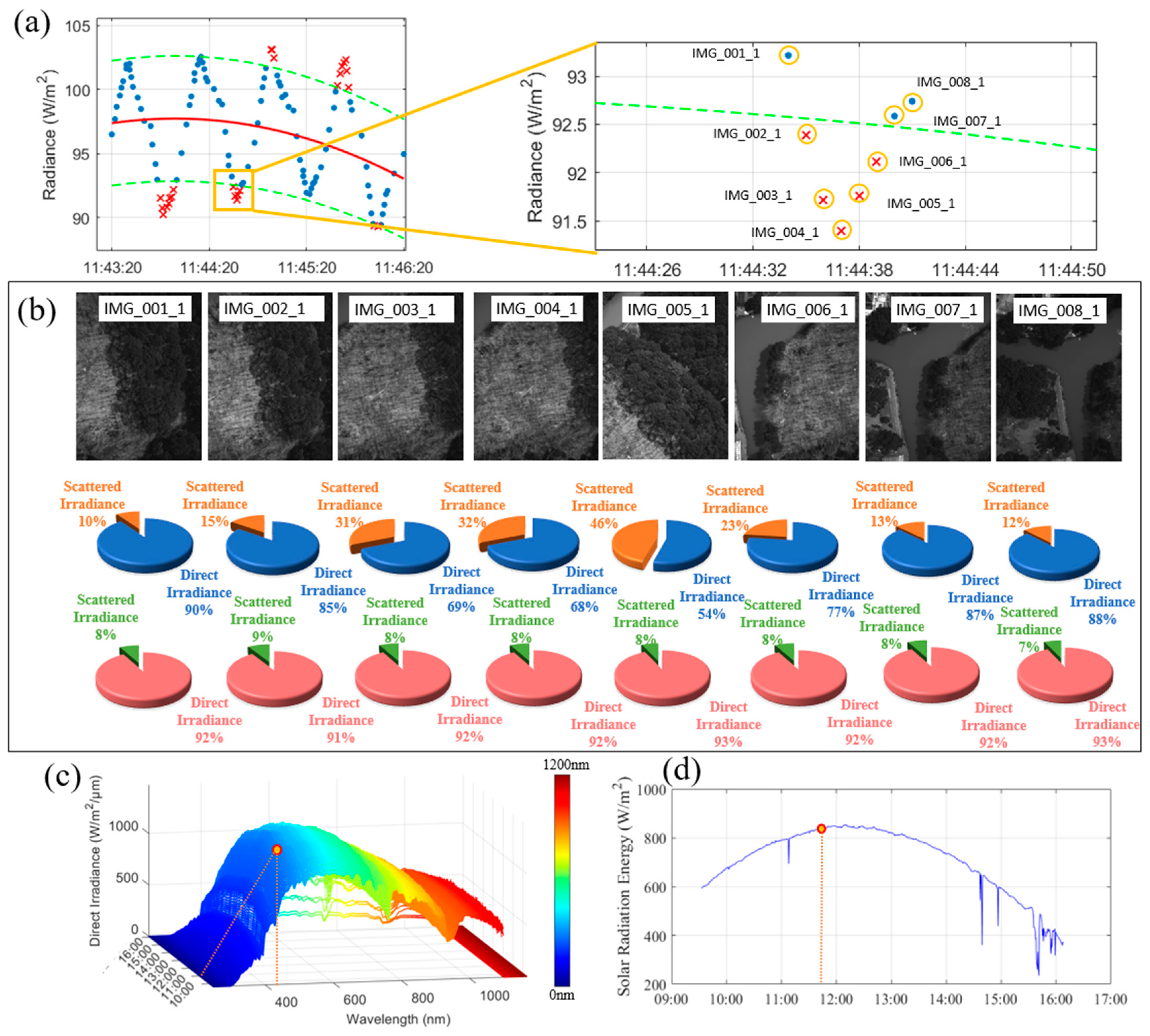
5.2. Analysis of Direct and Scattered Radiation Proportions in DLS Data

The total irradiance recorded by the DLS consists of two components: Scattered Irradiance and Direct Irradiance. Under stable and clear weather conditions, solar radiation remains relatively constant over short periods (approximately 30–40 min). Therefore, by analyzing the Scattered Irradiance and Direct Irradiance recorded by the DLS, it is possible to determine whether any anomalies in the DLS data are caused by abnormal UAV attitudes. Figure 9 presents a set of selected abnormal data, the corresponding image, and the proportions of recorded Scattered and Direct Irradiance, which can assist in investigating the causes of DLS data anomalies.

Figure 9a presents the selected data, showing a total of eight images from the first spectral band, named IMG_001_1 to IMG_008_1, among which five images fall outside the acceptable range. The upper part of Figure 9b displays the corresponding images, and it is evident that the UAV made a turning maneuver between IMG_001_3 and IMG_006_1. Figure 9c and Figure 9d, respectively, show the data recorded by the Solar Radiometer and the MS-711 Spectroradiometer, along with the spatial positions corresponding to the selected images in Figure 9. From Figure 9c,d, it can be observed that for the entire day’s irradiance, both direct solar irradiance and total irradiance exhibit no significant anomalies and generally follow a sinusoidal variation in line with the solar elevation angle. Within a 30–40 min time frame, neither direct irradiance nor total irradiance shows substantial changes, implying that the ratio between Scattered Irradiance and Direct Irradiance should remain relatively stable. However, the lower part of Figure 9b shows that from IMG_001_3 to IMG_006_1, the ratio between Scattered and Direct Irradiance underwent a dramatic shift: the Scattered Irradiance proportion increased from approximately 15% to around 50%, while the Direct Irradiance dropped from about 85% to 50%. This indicates a significant fluctuation in the DLS data, caused by the increased Scattered Irradiance due to UAV tilt during the turning maneuver. After the turn, at IMG_007_1, the irradiance ratio returned to normal. Although FIM-DC is not capable of separately correcting the values of direct and scattered components, it can effectively correct the total irradiance recorded by the DLS, demonstrating the effectiveness of the FIM-DC method.

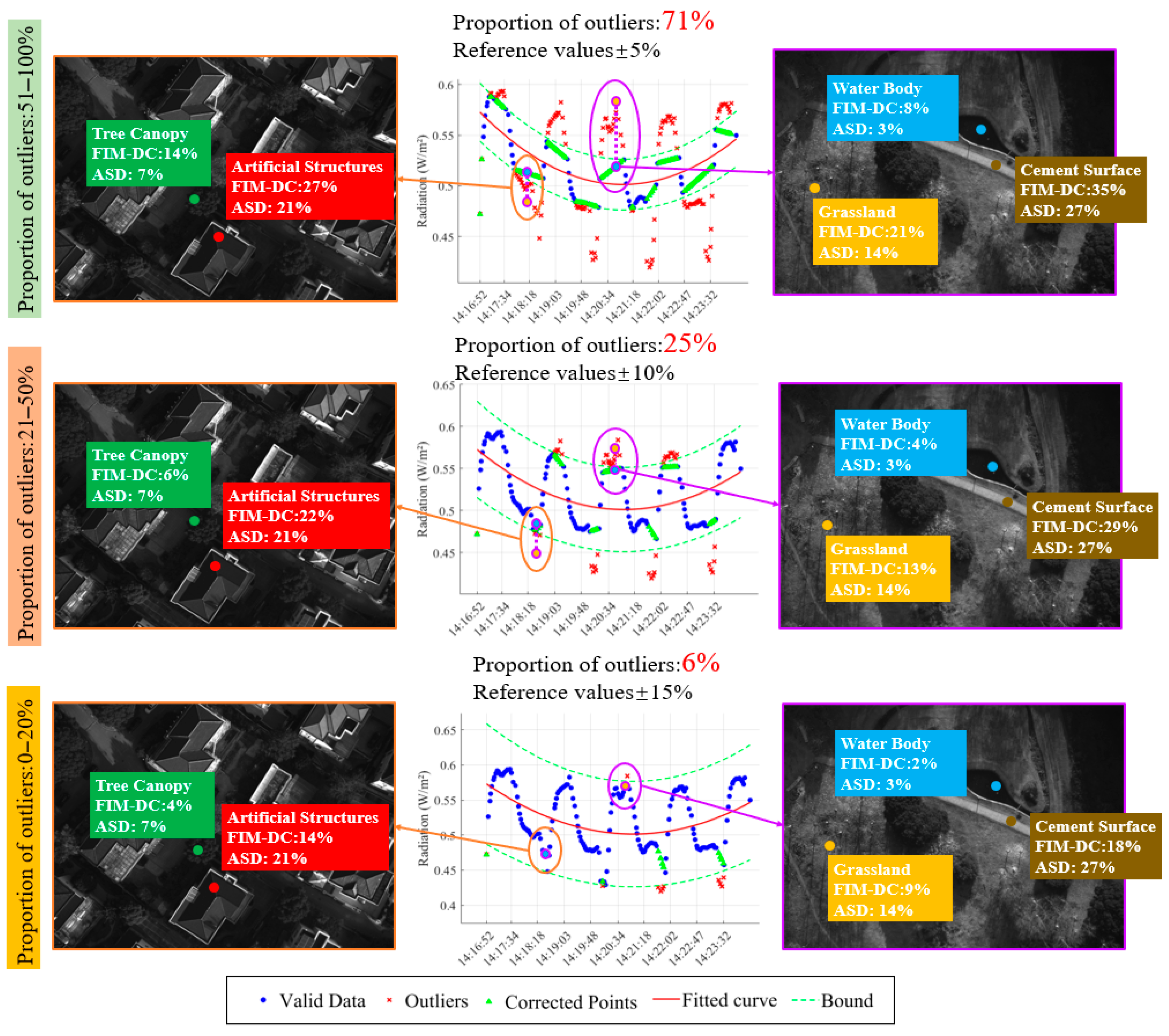
5.3. The Influence of Reference Values on the Model

The selection of parameters $Re{f}_{upper}$ and $Re{f}_{lower}$ is of critical importance. Different DLS datasets require distinct values of $Re{f}_{upper}$ and $Re{f}_{lower}$, as these parameters are influenced by various factors such as flight time, weather conditions, and UAV attitude.

To illustrate how a and b are set in different experimental scenarios, Figure 10 presents data from the Jiading test site, which is distinct from the previously discussed Qingpu site. Since the FIM-DC model identifies certain DLS data points as outliers, Figure 10 displays three separate cases where the proportion of outliers is set to 0–20%, 21–50%, and 51–100%, respectively. In the Jiading experiment, we used an ASD spectroradiometer to measure the reflectance of five typical land cover types—Tree Canopy, Grassland, Artificial Structures, Cement Surface, and Water Body—across six spectral bands. The measurements obtained by the ASD instrument are considered the ground-truth reflectance values of these surfaces. Figure 10 illustrates the true reflectance values in Band 3 for these five land cover types, as well as the corresponding reflectance values calculated by the FIM-DC model under different combinations of parameters $Re{f}_{upper}$ and $Re{f}_{lower}$. When the proportion of outliers was set to 5.79%, the reference range was defined as ±15% around the fitted curve, meaning that values within 15% of the curve were treated as acceptable. Under this configuration, the reflectance values estimated by the FIM-DC model were generally lower than the ASD-measured values. For instance, the reflectance of Cement Surface measured by the ASD spectroradiometer was 27%, while the FIM-DC result was only 18%. This discrepancy occurred because very few points were corrected, and the original abnormal reflectance values remained largely unmodified. In another case, when the proportion of outliers was set to 70.53%, the vast majority of points were treated as outliers, which is clearly incorrect. The results showed that this led to a significant overestimation of reflectance values. After multiple trials, it was found that setting the proportion of outliers within the range of 21% to 50% yielded the most reasonable results. Within this range, the estimated reflectance closely matched the ground-truth values. Experiments conducted in both the Jiading and Qingpu test areas consistently supported this conclusion.

6. Conclusions

This study explored a data correction method based on fitting and interpolation models called FIM-DC to improve the accuracy of UAV reflectance imagery derived from DLS data under clear-sky conditions. The research yielded the following key findings:

• Improved Reflectance Consistency: FIM-DC significantly reduced the standard deviation of reflectance at tie points across multiple spectral bands, with the most notable improvement decreasing from 15.07% to 0.58%, ensuring superior radiometric consistency in DOMs.
• Effective Anomaly Correction: The method successfully eliminated abrupt fluctuations in DLS data caused by UAV attitude anomalies, achieving seamless mosaicking of large-area reflectance DOMs.
• Radiation Component Analysis: Through detailed examination of direct and scattered radiation proportions, the study identified the root causes of DLS anomalies during UAV maneuvers, providing critical insights for sensor optimization.
• Spectral Performance: FIM-DC accurately corrected spectral curves for six land cover types, reducing reflectance discrepancies by up to 15% in key spectral bands between anomalous and normal images.

FIM-DC provides a reliable and efficient computational solution for reflectance calculation using DLS data in UAV remote sensing. By effectively addressing anomalies caused by UAV attitude fluctuations, FIM-DC ensures high radiometric consistency across large-scale mosaicked reflectance images. The method shows significant potential for practical applications in agricultural monitoring, forest management, and environmental surveying. To comprehensively assess the robustness and generalizability of the FIM-DC model, future research should explore its performance across more diverse terrains, land cover types, and under variable atmospheric and illumination conditions. Moreover, the development of real-time correction frameworks and their integration into onboard processing systems would further enhance the operational value of FIM-DC for high-frequency UAV missions and time-sensitive field applications.

References

1. Román, A.; Tovar-Sánchez, A.; Olivé, I.; Navarro, G. Using a UAV-Mounted Multispectral Camera for the Monitoring of Marine Macrophytes. Front. Mar. Sci. 2021, 8, 722698. [Google Scholar] [CrossRef]
2. Swaminathan, V.; Thomasson, J.A.; Hardin, R.G.; Rajan, N.; Raman, R. Radiometric Calibration of UAV Multispectral Images under Changing Illumination Conditions with a Downwelling Light Sensor. Plant Phenome J. 2024, 7, e70005. [Google Scholar] [CrossRef]
3. Hakala, T.; Markelin, L.; Honkavaara, E.; Scott, B.; Theocharous, T.; Nevalainen, O.; Näsi, R.; Suomalainen, J.; Viljanen, N.; Greenwell, C.; et al. Direct Reflectance Measurements from Drones: Sensor Absolute Radiometric Calibration and System Tests for Forest Reflectance Characterization. Sensors 2018, 18, 1417. [Google Scholar] [CrossRef]
4. Zhao, F.; Sun, R.; Zhong, L.; Meng, R.; Huang, C.; Zeng, X.; Wang, M.; Li, Y.; Wang, Z. Monthly Mapping of Forest Harvesting Using Dense Time Series Sentinel-1 SAR Imagery and Deep Learning. Remote Sens. Environ. 2022, 269, 112822. [Google Scholar] [CrossRef]
5. Hunt, E.R.; Stern, A.J. Evaluation of Incident Light Sensors on Unmanned Aircraft for Calculation of Spectral Reflectance. Remote Sens. 2019, 11, 2622. [Google Scholar] [CrossRef]
6. Liu, Y.; Shan, Y.; Ying, H.; Wala, D.; Zhang, X.; Ruhan, A.; Rina, S.; Rina, S. Examining the Angular Effects of UAV-LS on Vegetation Metrics Using a Framework for Mediating Effects. Forests 2022, 13, 1221. [Google Scholar] [CrossRef]
7. Daniels, L.; Eeckhout, E.; Wieme, J.; Dejaegher, Y.; Audenaert, K.; Maes, W.H. Identifying the Optimal Radiometric Calibration Method for UAV-Based Multispectral Imaging. Remote Sens. 2023, 15, 2909. [Google Scholar] [CrossRef]
8. Cottrell, B.; Kalacska, M.; Arroyo-Mora, J.-P.; Lucanus, O.; Inamdar, D.; Løke, T.; Soffer, R.J. Limitations of a Multispectral UAV Sensor for Satellite Validation and Mapping Complex Vegetation. Remote Sens. 2024, 16, 2463. [Google Scholar] [CrossRef]
9. Lu, H.; Fan, T.; Ghimire, P.; Deng, L. Experimental Evaluation and Consistency Comparison of UAV Multispectral Minisensors. Remote Sens. 2020, 12, 2542. [Google Scholar] [CrossRef]
10. Suomalainen, J.; Hakala, T.; Alves De Oliveira, R.; Markelin, L.; Viljanen, N.; Näsi, R.; Honkavaara, E. A Novel Tilt Correction Technique for Irradiance Sensors and Spectrometers On-Board Unmanned Aerial Vehicles. Remote Sens. 2018, 10, 2068. [Google Scholar] [CrossRef]
11. Sekrecka, A.; Wierzbicki, D.; Kedzierski, M. Influence of the Sun Position and Platform Orientation on the Quality of Imagery Obtained from Unmanned Aerial Vehicles. Remote Sens. 2020, 12, 1040. [Google Scholar] [CrossRef]
12. Stow, D.; Nichol, C.; Wade, T.; Assmann, J.; Simpson, G.; Helfter, C. Illumination Geometry and Flying Height Influence Surface Reflectance and NDVI Derived from Multispectral UAS Imagery. Drones 2019, 3, 55. [Google Scholar] [CrossRef]
13. James, M.R.; Robson, S. Mitigating Systematic Error in Topographic Models Derived from UAV and Ground-based Image Networks. Earth Surf. Process. Landf. 2014, 39, 1413–1420. [Google Scholar] [CrossRef]
14. Turner, D.; Lucieer, A.; Watson, C. An Automated Technique for Generating Georectified Mosaics from Ultra-High Resolution Unmanned Aerial Vehicle (UAV) Imagery, Based on Structure from Motion (SfM) Point Clouds. Remote Sens. 2012, 4, 1392–1410. [Google Scholar] [CrossRef]
15. Simon, N.; Ren, A.Z.; Piqué, A.; Snyder, D.; Barretto, D.; Hultmark, M.; Majumdar, A. FlowDrone: Wind Estimation and Gust Rejection on UAVs Using Fast-Response Hot-Wire Flow Sensors. In Proceedings of the 2023 IEEE International Conference on Robotics and Automation (ICRA), London, UK, 29 May–2 June 2023. [Google Scholar]
16. Jung, S. Precision Landing of Unmanned Aerial Vehicle under Wind Disturbance Using Derivative Sliding Mode Nonlinear Disturbance Observer-Based Control Method. Aerospace 2024, 11, 265. [Google Scholar] [CrossRef]
17. Köppl, C.J.; Malureanu, R.; Dam-Hansen, C.; Wang, S.; Jin, H.; Barchiesi, S.; Serrano Sandí, J.M.; Muñoz-Carpena, R.; Johnson, M.; Durán-Quesada, A.M.; et al. Hyperspectral Reflectance Measurements from UAS under Intermittent Clouds: Correcting Irradiance Measurements for Sensor Tilt. Remote Sens. Environ. 2021, 267, 112719. [Google Scholar] [CrossRef]
18. Reineman, B.D.; Lenain, L.; Statom, N.M.; Melville, W.K. Development and Testing of Instrumentation for UAV-Based Flux Measurements within Terrestrial and Marine Atmospheric Boundary Layers. J. Atmos. Ocean. Technol. 2013, 30, 1295–1319. [Google Scholar] [CrossRef]
19. Deng, L.; Hao, X.; Mao, Z.; Yan, Y.; Sun, J.; Zhang, A. A Subband Radiometric Calibration Method for UAV-Based Multispectral Remote Sensing. IEEE J. Sel. Top. Appl. Earth Obs. Remote Sens. 2018, 11, 2869–2880. [Google Scholar] [CrossRef]
20. Xue, B.; Ming, B.; Xin, J.; Yang, H.; Gao, S.; Guo, H.; Feng, D.; Nie, C.; Wang, K.; Li, S. Radiometric Correction of Multispectral Field Images Captured under Changing Ambient Light Conditions and Applications in Crop Monitoring. Drones 2023, 7, 223. [Google Scholar] [CrossRef]
21. Wang, Y.; Yang, Z.; Khan, H.A.; Kootstra, G. Improving Radiometric Block Adjustment for UAV Multispectral Imagery under Variable Illumination Conditions. Remote Sens. 2024, 16, 3019. [Google Scholar] [CrossRef]
22. Meier, K.; Hann, R.; Skaloud, J.; Garreau, A. Wind Estimation with Multirotor UAVs. Atmosphere 2022, 13, 551. [Google Scholar] [CrossRef]
23. Wilson, T.C.; Brenner, J.; Morrison, Z.; Jacob, J.D.; Elbing, B.R. Wind Speed Statistics from a Small UAS and Its Sensitivity to Sensor Location. Atmosphere 2022, 13, 443. [Google Scholar] [CrossRef]
24. Palomaki, R.T.; Rose, N.T.; Van Den Bossche, M.; Sherman, T.J.; De Wekker, S.F.J. Wind Estimation in the Lower Atmosphere Using Multirotor Aircraft. J. Atmos. Ocean. Technol. 2017, 34, 1183–1191. [Google Scholar] [CrossRef]
25. LaForest, L.; Hasheminasab, S.M.; Zhou, T.; Flatt, J.E.; Habib, A. New Strategies for Time Delay Estimation during System Calibration for UAV-Based GNSS/INS-Assisted Imaging Systems. Remote Sens. 2019, 11, 1811. [Google Scholar] [CrossRef]
26. He, X.; Zhang, X.; Tang, L.; Liu, W. Instantaneous Real-Time Kinematic Decimeter-Level Positioning with BeiDou Triple-Frequency Signals over Medium Baselines. Sensors 2015, 16, 1. [Google Scholar] [CrossRef] [PubMed]
27. Zhukov, I.; Dolintse, B.; Balakin, S. Enhancing Data Processing Methods to Improve UAV Positioning Accuracy. Int. J. Image Graph. Signal Process. 2024, 16, 100–110. [Google Scholar] [CrossRef]
28. Bramati, M.; Schön, M.; Schulz, D.; Savvakis, V.; Wang, Y.; Bange, J.; Platis, A. A Versatile Calibration Method for Rotary-Wing UAS as Wind Measurement Systems. J. Atmos. Ocean. Technol. 2024, 41, 25–43. [Google Scholar] [CrossRef]
29. Yang, Y.; Kim, S.; Lee, K.; Leeghim, H. Disturbance Robust Attitude Stabilization of Multirotors with Control Moment Gyros. Sensors 2024, 24, 8212. [Google Scholar] [CrossRef]
30. Chiang, K.-W.; Tsai, M.-L.; Naser, E.-S.; Habib, A.; Chu, C.-H. New Calibration Method Using Low Cost MEM IMUs to Verify the Performance of UAV-Borne MMS Payloads. Sensors 2015, 15, 6560–6585. [Google Scholar] [CrossRef]
31. Xie, J.; Shen, Y.; Cen, H. Real-Time Reflectance Generation for UAV Multispectral Imagery Using an Onboard Downwelling Spectrometer in Varied Weather Conditions. arXiv 2024, arXiv:2412.19527. [Google Scholar]
32. Paul, S.; Nagesh Kumar, D. Spectral-Spatial Classification of Hyperspectral Data with Mutual Information Based Segmented Stacked Autoencoder Approach. ISPRS J. Photogramm. Remote Sens. 2018, 138, 265–280. [Google Scholar] [CrossRef]
33. D’Amico, S.; Ardaens, J.-S.; Gaias, G.; Benninghoff, H.; Schlepp, B.; Jørgensen, J.L. Noncooperative Rendezvous Using Angles-Only Optical Navigation: System Design and Flight Results. J. Guid. Control Dyn. 2013, 36, 1576–1595. [Google Scholar] [CrossRef]
34. Xu, L.; Cai, Z.; Wang, Y.; Shen, Z. The Control Method of a Quadrotor Driven by Bidirectional Electronic Speed Controllers. Sci. Rep. 2024, 14, 19532. [Google Scholar] [CrossRef]
35. Torrente, G.; Kaufmann, E.; Fohn, P.; Scaramuzza, D. Data-Driven MPC for Quadrotors. IEEE Robot. Autom. Lett. 2021, 6, 3769–3776. [Google Scholar] [CrossRef]
36. Smith, M.W.; Carrivick, J.L.; Quincey, D.J. Structure from Motion Photogrammetry in Physical Geography. Prog. Phys. Geogr. Earth Environ. 2016, 40, 247–275. [Google Scholar] [CrossRef]
37. Yue, J.; Lei, T.; Li, C.; Zhu, J. The Application of Unmanned Aerial Vehicle Remote Sensing in Quickly Monitoring Crop Pests. Intell. Autom. Soft Comput. 2012, 18, 1043–1052. [Google Scholar] [CrossRef]
38. Zhang, R.; Hewitt, A.; Li, L.; Yuan, H.; Ferguson, J.C.; Chen, L. Editorial: Advanced Technologies of UAV Application in Crop Pest, Disease and Weed Control. Front. Plant Sci. 2023, 14, 1253841. [Google Scholar] [CrossRef] [PubMed]
39. Miller, J.K.; Dean, R.G. A Simple New Shoreline Change Model. Coast. Eng. 2004, 51, 531–556. [Google Scholar] [CrossRef]
40. Polat, N.; Memduhoğlu, A. Assessing Spatiotemporal LST Variations in Urban Landscapes Using Diurnal UAV Thermography. Appl. Sci. 2025, 15, 3448. [Google Scholar] [CrossRef]
41. Navarro-Gutiérrez, M.; Ramírez-Treviño, A.; Silva, M. Fluid Net Models: From Behavioral Properties to Structural Objects. Appl. Sci. 2022, 12, 6123. [Google Scholar] [CrossRef]
42. Shin, H.J.; Park, J.; Lee, J.S. Syllable-Based Multi-POSMORPH Annotation for Korean Morphological Analysis and Part-of-Speech Tagging. Appl. Sci. 2023, 13, 2892. [Google Scholar] [CrossRef]
43. Zhu, S.; Guan, H.; Millington, A.C.; Zhang, G. Disaggregation of Land Surface Temperature over a Heterogeneous Urban and Surrounding Suburban Area: A Case Study in Shanghai, China. Int. J. Remote Sens. 2013, 34, 1707–1723. [Google Scholar] [CrossRef]
44. Zakšek, K.; Oštir, K. Downscaling Land Surface Temperature for Urban Heat Island Diurnal Cycle Analysis. Remote Sens. Environ. 2012, 117, 114–124. [Google Scholar] [CrossRef]
45. Rodrigues De Almeida, C.; Garcia, N.; Campos, J.C.; Alírio, J.; Arenas-Castro, S.; Gonçalves, A.; Sillero, N.; Teodoro, A.C. Time-Series Analyses of Land Surface Temperature Changes with Google Earth Engine in a Mountainous Region. Heliyon 2023, 9, e18846. [Google Scholar] [CrossRef] [PubMed]
46. Hochreiter, S.; Schmidhuber, J. Long Short-Term Memory. Neural Comput. 1997, 9, 1735–1780. [Google Scholar] [CrossRef]
47. Tamiminia, H.; Salehi, B.; Mahdianpari, M.; Quackenbush, L.; Adeli, S.; Brisco, B. Google Earth Engine for Geo-Big Data Applications: A Meta-Analysis and Systematic Review. ISPRS J. Photogramm. Remote Sens. 2020, 164, 152–170. [Google Scholar] [CrossRef]
Figure 1. Schematic diagram of the FIM-DC model: (a) illustration of DLS data; (b) schematic diagram of the FIM-DC model method.
Drones 09 00491 g001
Figure 2. Experimental flowchart.
Drones 09 00491 g002
Figure 3. Experimental area geographic location and flight path.
Drones 09 00491 g003
Figure 4. Experimental equipment: (a) DJI M300 UAV (SZ DJI Technology Co., Ltd., Shenzhen, China); (b) Altum-PT multispectral camera (MicaSense, Inc., Seattle, WA, USA); (c) downwelling light sensor (MicaSense, Inc., Seattle, WA, USA); (d) solar radiometer (Apogee Instruments, Inc., Logan, UT, USA); (e) MS-711 spectroradiometer (Malvern Panalytical Ltd., Malvern, UK).
Drones 09 00491 g004
Figure 5. Reflectance of four land cover types in Band 1.
Drones 09 00491 g005
Figure 6. Reflectance of four land cover types in Band 4.
Drones 09 00491 g006
Figure 7. Comparison of stitching effects: (a) DLS data selection; (b) stitched images and flight paths; (c) local zoomed comparison.
Drones 09 00491 g007
Figure 8. Comparison of spectral curves for six land cover types: (a) location map of selected images; (b) locations of selected land cover types; (c) spectral curve comparison.
Drones 09 00491 g008
Figure 9. Analysis of scattered irradiance and direct irradiance proportions: (a) selected image data; (b) proportions of scattered and direct irradiance with corresponding images; (c) radiometric data; (d) solar irradiance data.
Drones 09 00491 g009
Figure 10. Effect of different parameter R e f u p p e r and R e f l o w e r selections on the reflectance.
Drones 09 00491 g010