An Efficient Autonomous Exploration Framework for Autonomous Vehicles in Uneven Off-Road Environments

Abstract

Autonomous exploration of autonomous vehicles in off-road environments remains challenging due to the adverse impact on exploration efficiency and safety caused by uneven terrain. In this paper, we propose a path planning framework for autonomous exploration to obtain feasible and smooth paths for autonomous vehicles in 3D off-road environments. In our framework, we design a target selection strategy based on 3D terrain traversability analysis, and the traversability is evaluated by integrating vehicle dynamics with geometric indicators of the terrain. This strategy detects the frontiers within 3D environments and utilizes the traversability cost of frontiers as the pivotal weight within the clustering process, ensuring the accessibility of candidate points. Additionally, we introduced a more precise approach to evaluate navigation costs in off-road terrain. To obtain a smooth local path, we generate a cluster of local paths based on the global path and evaluate the optimal local path through the traversability and smoothness of the path. The method is validated in simulations and real-world environments based on representative off-road scenarios. The results demonstrate that our method reduces the exploration time by up to 36.52% and ensures the safety of the vehicle while exploring unknown 3D off-road terrain compared with state-of-the-art methods.

1. Introduction

The problem of autonomous exploration has attracted much interest regarding various robotic systems in recent decades [1,2]. Autonomous exploration in off-road environments is of great significance for practical applications, such as planetary exploration [3] and search and rescue (SAR) [4], where robots work on rugged and challenging terrain. However, autonomous exploration methods for autonomous vehicles in off-road environments must consider both terrain traversability and nonholonomic constraints, and thus present more challenges than methods for on-road environments.

As the core component of autonomous exploration, path planning aims to determine “where to go and how to get there” in unknown environments and generate a feasible path for vehicles to traverse the entire environment. However, most path planning methods for exploration have been applied to indoor environments with clearly structured features or have been demonstrated in flat road environments [5]. These methods still have several limitations in off-road environments dominated by uneven terrain. Path planning of exploration in off-road environments presents additional challenges. First, the off-road environment is highly complex, making it challenging to accurately describe obstacles. Unlike in urban cities, natural elements such as plants, rocks, potholes, and cliffs are difficult to identify due to their irregular shapes and random distributions, rendering simple binary classification impractical [6]. As a result, the traditional binary representation of obstacles is not well suited for off-road environments. Second, some motion planning methods for autonomous vehicles in off-road environments incorporate terrain analysis modules to address the challenges of path planning in complex terrains [7,8]. However, most existing approaches only utilize traversability information to avoid untraversable terrain but do not fully integrate it into the design of exploration strategies. If exploration targets are in regions that are difficult or risky for the vehicle to reach, it may hinder mission completion and potentially compromise the vehicle’s safety. Additionally, both nonholonomic constraints and the rugged terrain limit the speed of vehicles. If the path passes through rugged terrain, it will be detrimental to the vehicle’s safety and exploration efficiency. Furthermore, it also reduces the accuracy of exploration mapping [9]. Vehicular vibrations caused by uneven terrain may compromise the measurement precision of the sensors, affecting the accuracy of the constructed map. However, few methods consider the traversability cost when computing exploration paths.

This paper overcomes the above challenges by proposing an efficient path planning method for exploration that considers the cost of terrain traversability, as shown in Figure 1. The traversability cost is evaluated by integrating the vehicle dynamics parameters with geometric indicators of the terrain, including slope, roughness, and sparsity. To optimize the computational efficiency of environment modeling in 3D uneven space, we establish a multi-resolution layered grid map to store environmental information required by exploration planning, including point cloud data, traversability cost, and exploration state. Motivated by [10], we extend frontier detection to 3D space to track state changes of exploration. Additionally, we introduce quantified traversability cost into frontier clustering and target evaluation, enabling the selected targets to be accessible to the vehicle. The corresponding path generated during the evaluation process is termed the global path. To achieve a smooth local path, we employ the cubic spiral to generate a series of smooth paths based on the global path and utilize the traversability cost of the path as a parameter to evaluate the path cluster. We conduct comparative simulation experiments with classic and state-of-the-art methods in different environments. The results show that our method completes exploration with a lower traversability cost and the highest average vehicle speed. Furthermore, we conduct experiments in real-world scenarios to demonstrate the capability of our method to support efficient and safe exploration in uneven off-road environments.

The contributions of this paper can be summarized as follows:

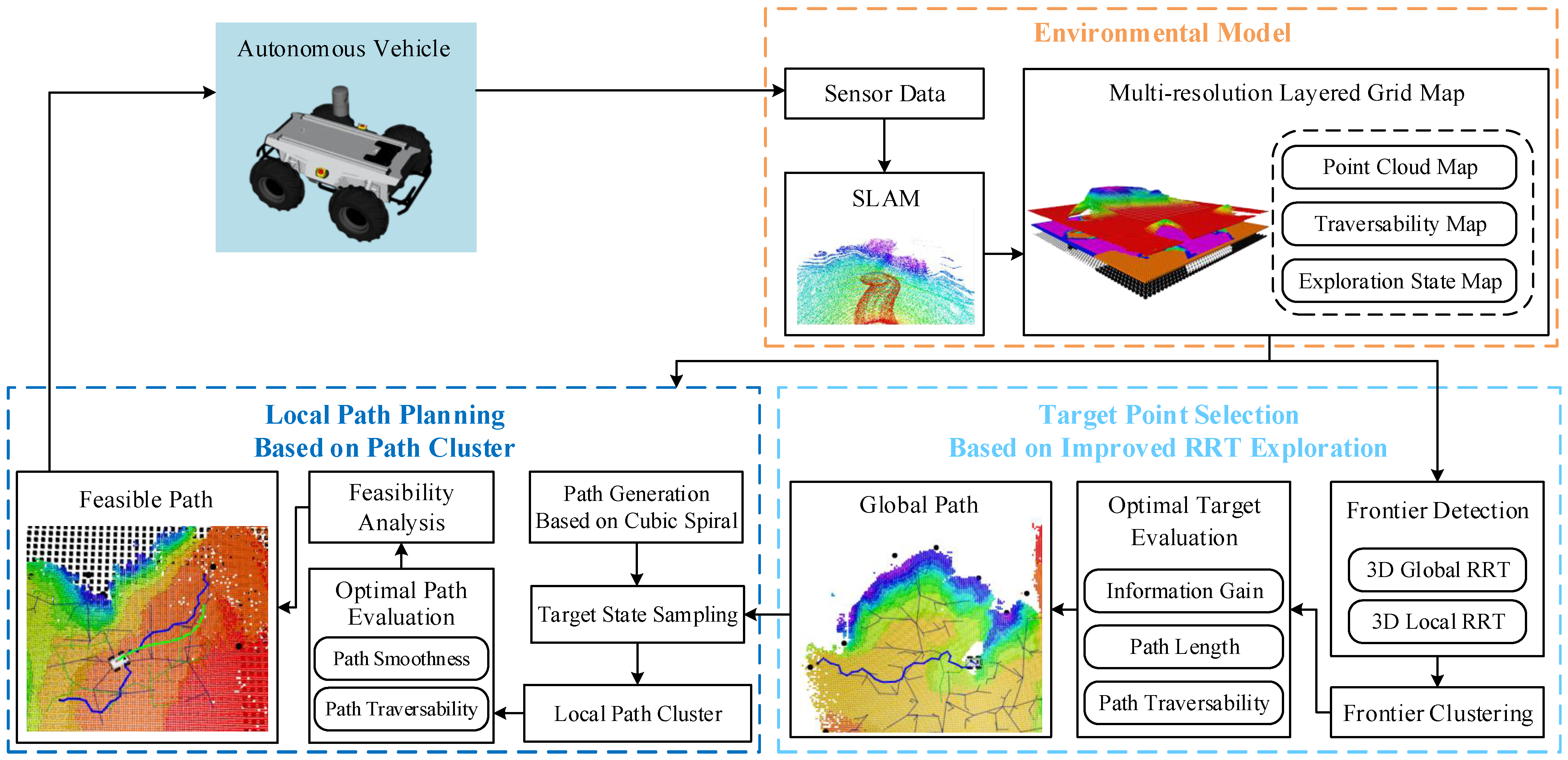
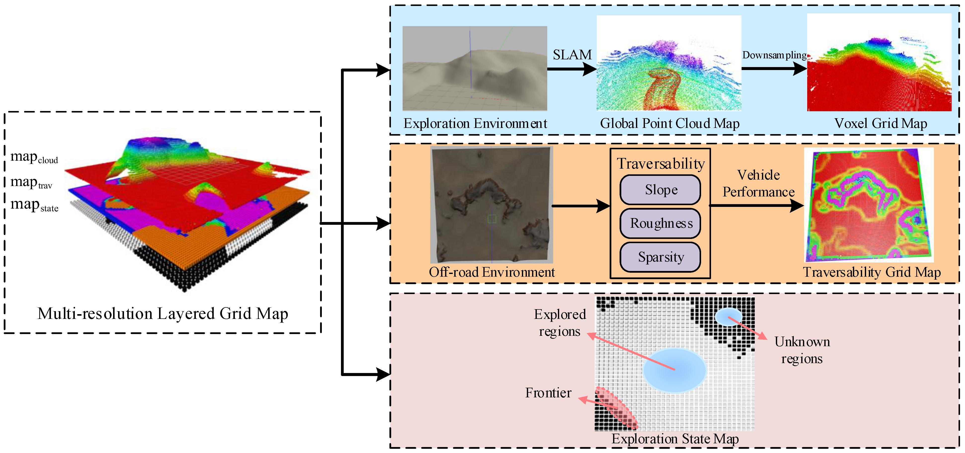
• A multi-resolution layered map serves as the environmental model for exploration, storing environmental information at various resolutions for efficient storage resource allocation.
• A target selection strategy that considers terrain traversability analysis ensures the accessibility of the target within 3D uneven off-road environments. Furthermore, we determine the optimal target by integrating information gain with a more precise navigation cost.
• A local path planner integrates path traversability to select the optimal local path from the smooth candidate paths, ensuring that the local path is optimally suited for the vehicle’s traversal while meeting kinematic constraints and enhancing exploration efficiency and the vehicle’s safety in off-road environments.

2. Related Work

2.1. Methods of Autonomous Exploration

The development of autonomous driving technology has significantly promoted the research of autonomous exploration. The exploration techniques can be classified into four primary categories [11,12]: frontier-based methods, Next Best View (NBV)-based methods, information theory-based methods, and learning-based methods. We only discuss the previous two methods, which have been widely used in various exploration tasks.

Frontier-based methods aim to guide vehicles towards unknown regions by identifying the frontier between the explored and unexplored areas in the environment and selecting the optimal frontier point. Frontier-based methods can provide strong guidance for the exploration of vehicles. To address the challenges of decreasing the efficiency of frontier detection and trapping exploration in local optima, researchers have primarily conducted extensive studies on methods of frontier detection and strategies of frontier selection [13,14]. Although frontier-based approaches have a common application in exploration, the efficiency of frontier detection decreases as the exploration environment expands, especially in three-dimensional environments.

NBV-based methods utilize random sampling algorithms, such as Rapidly exploring Random Tree (RRT), to sample viewpoints around the vehicle. By quantifying the exploration gain against the travel cost for each viewpoint, these methods select the viewpoint with the highest expected gain as the target [15]. NBV-based methods facilitate the quick generation of maps in the early phases of exploration. However, these methods have less attention on areas offering small gains. Consequently, these smaller areas might be neglected throughout the exploration, increasing the risk of falling into local minima [16].

2.2. Autonomous Exploration in 3D Environments

As exploration methods in 2D environments are insufficient to satisfy the requirements for exploration in complex environments, researchers have dedicated their efforts to exploration in 3D environments.

Several scholars achieve exploration in 3D environments by improving detection and selection for frontier points or viewpoints. Dang et al. [17] propose a strategy for visual saliency-aware receding horizon exploration and planned the path to the viewpoint using a visual attention model, optimizing the attention of environmentally salient features. Unfortunately, this method is only tested in indoor environments and may not perform effectively in off-road environments with more complex terrain features. To enhance exploration efficiency, Batinovic [18] uses point cloud data processed by the Cartographer to construct the octree map, effectively filtering frontier points by adjusting resolution. FUEL [19] reduces candidate frontiers using an incremental frontier information structure (FIS) and generates efficient paths by sampling viewpoints with high coverage and solving the asymmetric traveling salesman problem (ATSP). However, these methods may lead the robot to neglect low-information-gain regions in the early stages of exploration, resulting in more revisit time. To address this issue, UFOExplorer [20] constructs a dynamic undirected graph and navigates toward the nearest informative viewpoint, avoiding the potential oversight of low-information-gain areas. However, it is worth noting that the exploration method for uneven terrain requires considering not only the efficiency but also the navigation safety of the robot. To cope with uneven terrains, some prior methods introduce terrain analysis modules. Refs. [21,22] employ the point cloud to construct an elevation map, and they are prone to misidentify undulating terrains as untraversable areas, which results in incomplete extraction of potentially explorable unknown regions near undulating terrains. The work in [23] incorporates a more detailed traversability analysis by considering terrain features and classifying paths as either traversable or untraversable. However, it does not further consider traversability cost during the exploration process.

Exploration methods based on a hybrid strategy also contribute to exploration in 3D environments, but few of them consider terrain traversability during navigation. The DSVP method [24] uses local frontiers as the direction for RRT expansion and considers nodes of the RRT as viewpoints, resulting in more viewpoints close to the current exploration direction. Chen et al. [25] propose a local planner to efficiently explore unknown areas within the field of view (FoV) by combining frontier-based and NBV-based methods, enhancing the effectiveness of autonomous exploration tasks. Li et al. [26] present a visual exploration approach that integrates learning-augmented model-based planning with the frontier-based exploration method, using CNNs to forecast the characteristics of uncharted territories and enhance exploration coverage. However, the method was only tested on indoor datasets, and its generalization capability remains to be further validated.

Additionally, most methods only ensure that the selected exploration targets avoid obstacles without considering whether the vehicle can reach them. To address this, Tang et al. [27] construct the 3D environment as a 2D accessibility map to ensure the accessibility of frontier points. However, they fail to account for the traversability of the environment during the path planning process, which can be fatal for autonomous exploration in off-road environments. In contrast, our method not only constructs the traversability map to ensure the accessibility of generated targets but also incorporates terrain traversability into target selection and path planning. This comprehensive approach significantly boosts the safety and efficiency of vehicle exploration in challenging off-road terrains.

3. Problem Definition

Let the workspace of the vehicle be V. Autonomous exploration seeks to maximize the total observation space $V_{\mathrm{total}}$, making $V_{\mathrm{total}}$ as close as possible to V when the vehicle completes the exploration. Traditional exploration methods typically classify the state space of the environment into free space $V_{\mathrm{free}}$ and occupied space $V_{\mathrm{occ}}$. This classification method has certain limitations for exploration in unknown off-road environments. Due to the blurred boundaries between roads and obstacles, it is challenging to strictly define the traversable area for vehicles. Thus, it is impractical to divide the state space solely based on free and occupied states. Considering that vehicles with different performances exhibit various maneuverability in off-road terrain, this paper defines the problem of autonomous exploration for vehicles in off-road environments as follows:

Definition 1 (Environmental Space): Define the state of the 3D workspace ($V\subset {\mathbb{R}}^3$) initially as unknown. During the exploration, we divide the space into the traversable subspace $V_{\mathrm{trav}}$ and the untraversable subspace $V_{\mathrm{untrav}}$. The determination of $V_{\mathrm{trav}}$ and $V_{\mathrm{untrav}}$ depends on the assessment of terrain traversability.

Definition 2 (Path Planning): Given the initial position ${\epsilon }_{\mathrm{init}}\in V_{\mathrm{trav}}$, the vehicle perceives the surroundings and plans a path $\Gamma$ to explore the workspace:

$$\Gamma \ast =arg\underset{\Gamma }{min}(V-V_{total}(\Gamma ))$$

(1)

where $V_{total}(\Gamma )$ is the cumulative observation space of the vehicle after executing the path $\Gamma$. $\Gamma$ should satisfy (1) kinematic and dynamic constraints of the vehicle; (2) collision avoidance with obstacles and untraversable terrain to ensure safety; (3) maximizing the traversability of $\Gamma$ to enhance the speed of the vehicle.

4. Methodology

4.1. Environmental Model Construction

To simplify the environmental modeling of off-road environments, we construct a multi-resolution layered grid map for exploration. As shown in Figure 2, the model consists of the point cloud map $ma{p}_{\mathrm{cloud}}$, the exploration state map $ma{p}_{\mathrm{state}}$, and the traversability map $ma{p}_{\mathrm{trav}}$. This approach saves storage space by representing the environment with various resolutions and facilitates faster access to relevant information to enhance the efficiency and effectiveness of exploration. $ma{p}_{\mathrm{cloud}}$ stores the surface point clouds of the explored environment in the form of 3D voxel grids. This allows for a detailed representation of off-road terrain features and provides 3D terrain information for path planning to ensure vehicle’s safety. $ma{p}_{\mathrm{state}}$ indicates whether each grid is explored or unexplored. Points located near unexplored grids are defined as frontier points. The exploration mission is considered completed when there are almost no detectable frontier points. $ma{p}_{\mathrm{trav}}$ quantifies the traversability of each grid and provides crucial information for target selection and path planning during exploration. This contributes to preventing accidents such as rollover and overturning during driving.

To reduce the computation of traversability analysis and enhance the applicability of our method, we use vehicle’s dynamics parameters to represent the vehicle dynamics model. These parameters are the maximum terrain geometric indicators suitable for the vehicle, as determined by its dynamics model. This approach allows for efficient adaptation to various platforms by simply replacing the corresponding parameters for each new platform. We can obtain the traversability cost $\tau$ as follows:

$$\tau =\left\{\begin{array}{cc}1,& s\ge s_{max}\mathrm{or}r\ge r_{max}\mathrm{or}\lambda \ge {\lambda }_{max}\\ {\alpha }_1{\displaystyle \frac{s}{s_{max}}}+{\alpha }_2{\displaystyle \frac{r}{r_{max}}}+{\alpha }_3{\displaystyle \frac{\lambda }{{\lambda }_{max}}},& \mathrm{else}\end{array},\right.$$

(2)

where ${\alpha }_1$, ${\alpha }_2$, and ${\alpha }_3$ are weights that sum to 1, determining the relative influence of slope, roughness, and sparsity on the traversability cost. They can be adjusted according to the specific terrain characteristics of different scenarios. We calculate the terrain geometric indicators such as slope s, roughness r, and sparsity $\lambda$ using the method described in [28]. $s_{max}$, $r_{max}$, and ${\lambda }_{max}$ represent the maximum slope, roughness, and sparsity depending on the vehicle dynamic model, respectively. $\tau$ ranges from 0 to 1, with a higher $\tau$ indicating greater difficulty to traverse. If any indicator of the evaluated region exceeds its maximum, $\tau$ is assigned a value of 1, denoting that the region is untraversable for the vehicle.

Selecting an appropriate grid map resolution is complex and crucial. $ma{p}_{\mathrm{state}}$ mainly serves as a directional guide for target selection and does not require detailed information of the fine-scale area, so its resolution can be relatively coarse. In contrast, $ma{p}_{\mathrm{cloud}}$ provides crucial information for vehicles’ local path planning, ensuring vehicle safety and demands a relatively fine resolution. $ma{p}_{\mathrm{trav}}$ aims to evaluate the difficulty of navigating different regions relative to the vehicle, so its resolution should be determined based on the vehicle’s physical size for reducing the computational complexity of traversability cost.

4.2. Target Selection

To prevent the selected targets from being in areas that are difficult for vehicles to access, we propose a target selection strategy that considers the terrain traversability. This strategy confines candidates within accessible areas through frontier detection and clustering. Subsequently, the optimal targets are selected based on the proposed target evaluation function. In the subsequent content, we will detail the specific implementation for each section.

4.2.1. Frontier Detection

The RRT-based exploration [10] models the environment with a 2D grid map, which is inadequate to describe the complexity of 3D off-road terrains. Because the growth of an RRT is not affected by the spatial dimensions, we redefine the frontier detection method, which consists of a global RRT and a local RRT in 3D space.

Algorithm 1 presents the frontier detection process of the local RRT. The local RRT ${\mathcal{T}}_{\mathrm{local}}$ is first initialized at the start position of the vehicle. We define the tree nodes $\epsilon$ as 3D points and the plane points x as 2D points. At each iteration, the algorithm searches for node ${\epsilon }_{\mathrm{near}}$ that is closest to the sample plane point $x_{\mathrm{rand}}$ in ${\mathcal{T}}_{\mathrm{local}}$ and expands with the projection point $x_{\mathrm{near}}$ of ${\epsilon }_{\mathrm{near}}$ to obtain a new plane point $x_{\mathrm{new}}$ (Lines 3–6). Then, we use the function $LocalStateCheck\left(\right)$ to determine the state of $x_{\mathrm{new}}$. If the function returns $unknown$, indicating that $x_{\mathrm{new}}$ is a frontier point, it will be added to $\mathcal{F}$, and the local RRT will be reset to ${\epsilon }_{\mathrm{current}}$ (Lines 7–9). If the function returns $trav$, we will use function $ProjectToSurface\left(\right)$ to check whether the vehicle can reach $x_{\mathrm{new}}$. When $ProjectToSurface\left(x_{\mathrm{new}}\right)$ returns Ø, it indicates that the vehicle detects no surface point at $x_{\mathrm{new}}$, implying the possible presence of a negative obstacle. That means the vehicle cannot access $x_{\mathrm{new}}$, and the algorithm will enter the next iteration. Otherwise, the surface point ${\epsilon }_{\mathrm{new}}$ returned by the function will be connected to ${\mathcal{T}}_{\mathrm{local}}$ (Lines 10–15).

Algorithm 1: 3D Local RRT Frontier Detector

The global RRT is similar to the local RRT, with the main difference being the frontier detection method. The local tree aims to detect the surroundings of the vehicle efficiently, so it only requires evaluating whether $x_{\mathrm{new}}$ and the points on the line connecting $x_{\mathrm{new}}$ and $x_{\mathrm{near}}$ are frontier points. The global RRT is primarily designed to detect unknown regions in corners and far away. When there are points that qualify as the frontier in the vicinity of $x_{\mathrm{new}}$, $x_{\mathrm{new}}$ is a frontier point. This approach compensates for the shortcomings of the local detector. Additionally, unlike the local tree, the global tree does not require resetting after detecting frontier.

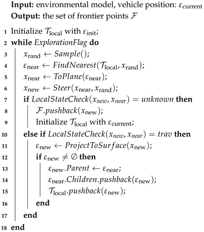
4.2.2. Frontier Clustering

To reduce the complexity of the evaluation, we filter and cluster the frontier points. Filtering is the process of removing invalid frontier points, which are points that no longer qualify as the frontier due to the movement of the vehicle. In this paper, we propose an improvement to the mean shift clustering algorithm [29] to ensure that the cluster centers are located in areas accessible to the vehicle. To achieve this, we use the traversability cost as a parameter to calculate the shift vector, which moves the cluster centers to the frontier points with low traversability cost.

The improved mean shift vector is as follows:

$$M_h\left(x\right)={\displaystyle \frac{\sum \left[T_h\left({∥\frac{x_i-x}{h}∥}^2\right)(x_i-x)\right]}{\sum T_h\left({∥\frac{x_i-x}{h}∥}^2\right)}},$$

(3)

$$T_h({∥{\displaystyle \frac{x_i-x}{h}}∥}^2)=\left\{\begin{array}{cc}N\left(\tau \left(x_i\right)\right),& {∥{\displaystyle \frac{x_i-x}{h}}∥}^2\le 1\\ 0,& \mathrm{else}\end{array},\right.$$

(4)

where $\tau \left(x_i\right)$ represents the traversability cost at the frontier point $x_i$. $N\left(x\right)={\displaystyle \frac{1}{\sqrt{2\pi }l}}{e}^{(-{\displaystyle \frac{x^2}{2l^2}})}$ is a Gaussian kernel function. Function $T_h(\ast )$ indicates that the frontier points, whose distance from the current cluster center is greater than the bandwidth h, do not influence the shift vector. Moreover, it ensures that the frontier points with better traversability will have more influence. Equation (3) allows the cluster center to move towards areas with better terrain traversability within the current bandwidth range during each iteration.

The detected frontier points can be clustered into several cluster centers, which have low traversability cost using the improved mean shift clustering algorithm. These centers are defined as candidate target points for the subsequent evaluation.

4.2.3. Optimal Target Evaluation

To determine which point in candidate target points could result in a faster and safer exploration, we define an evaluation function in Equation (5). This function selects the best exploration target by considering the information gain of each candidate point and the navigation cost required to reach it.

$$R={\beta }_1{\displaystyle \frac{g\left(P_i\right)I\left(P_i\right)}{{\sum }_{i=1}^{N_c}I\left(P_i\right)}}-{\beta }_2{\displaystyle \frac{C\left(P_i\right)}{{\sum }_{i=1}^{N_c}C\left(P_i\right)}},$$

(5)

$$g\left(P_i\right)=\left\{\begin{array}{cc}1,& dis\left(P_i\right)>\delta \\ g_{\mathrm{gain}},& \mathrm{else}\end{array},\right.$$

(6)

where ${\beta }_1$ and ${\beta }_2$ are the weights of the two decision variables, which determine the relative importance of information gain and navigation cost in target selection. Here, we normalize the information gain and navigation cost to remove their unit, where $N_c$ is the number of the candidate point. We quantify the information gain $I\left(P_i\right)$ at the candidate point $P_i$ using the area of unknown grids in the detection range. $C\left(P_i\right)$ is the navigation cost for the vehicle to travel to the candidate point $P_i$. The hysteretic gain $g\left(P_i\right)$ depends on the Euclidean distance $dis\left(P_i\right)$ between the vehicle and $P_i$, where $\delta$ is a distance threshold. $g_{\mathrm{gain}}>1$ makes vehicles biased to explore unknown areas in the vicinity to avoid overlapping.

Using Euclidean distance to represent navigation cost is simple, and it is inadequate in off-road environments. To achieve a more precise assessment of navigation cost in off-road terrains, we search the path to each candidate point and use the length cost and traversability cost of the obtained paths to obtain C, which possibly takes considerable computation time. Inspired by [30], we utilize the global and local RRT to construct a sparse 3D road map, facilitating faster path searching, as shown in Algorithm 2. The road map is represented by an undirected graph $\mathcal{R}=(\mathcal{V},E)$. The algorithm directly obtains new nodes from the global and local RRT during the exploration because these tree nodes are located in traversable areas and can be projected to the surface, reducing the need for redundant calculations. To ensure the sparsity of the road map, nodes are added to the road map only if their distance from the nearest node in $\mathcal{R}$ is greater than a specified threshold ${\zeta }_{dis}$. Then, we check the connectivity between each new node and their neighbors within specified radius $\gamma$.

Algorithm 2: 3D Road Map Construction

After constructing the 3D road map, the A* algorithm is employed to find feasible paths to candidate points, with the traversability cost for heuristic function. Thus, we construct a function to evaluate the navigation cost for the vehicle to each candidate point by considering the length and traversability of each path. Define $\mathrm{X}=\{{\epsilon }_1,{\epsilon }_2,\dots ,{\epsilon }_N\}$ as a path searched by A*, and ${\mathrm{X}}^{\prime }=\{x_0,x_1,x_2,\dots ,x_K\}$ is the path interpolated by X according to the resolution of $ma{p}_{\mathrm{trav}}$. We can obtain the length cost L of $\mathrm{X}$ as follows:

$$L=\sum _{i=1}^{N-1}∥{\epsilon }_{i+1}-{\epsilon }_i∥,$$

(7)

The traversability cost of $\mathrm{X}$ is

$$T=\left\{\begin{array}{cc}\infty ,& \exists k\in [0,K],\tau \left(x_k\right)=1\\ {\displaystyle \frac{{\tau }_{\mathrm{path}}}{K}},& \mathrm{else}\end{array},\right.$$

(8)

$${\tau }_{\mathrm{path}}=\sum _{i=0}^{K-1}(1+\sigma ({\displaystyle \frac{1}{1-\tau \left(x_i\right)}}+{\displaystyle \frac{1}{1-\tau \left(x_{i+1}\right)}}-2)),$$

(9)

where $\sigma$ is a penalty coefficient, typically set to 1. A larger value of $\sigma$ indicates higher traversability requirements for the path’s terrain, resulting in a greater traversability cost for the same path. $\tau \left(x_i\right)$ represents the traversability cost at the location corresponding to $x_i$, and $T\in (1,+\infty )$. The desired path to the target point should avoid areas that are hard to traverse while shortening the length, so we combine the length cost in Equation (7) and the traversability cost from Equation (8) to compute the navigation cost C.

$$C=T\ast L$$

(10)

By substituting the final navigation cost C into Equation (5), we can calculate the score for each candidate point. The point with the highest score is the optimal target point, and the corresponding path is defined as the global path.

4.3. Local Path Planning

Due to the final global path consisting of several edges of road map, it has poor smoothness. Note that it is difficult to directly optimize the 3D global path using existing methods. Inspired by a state space sampling-based strategy [31], we select the optimal local path from some smooth paths generated by sampling target states along the global path.

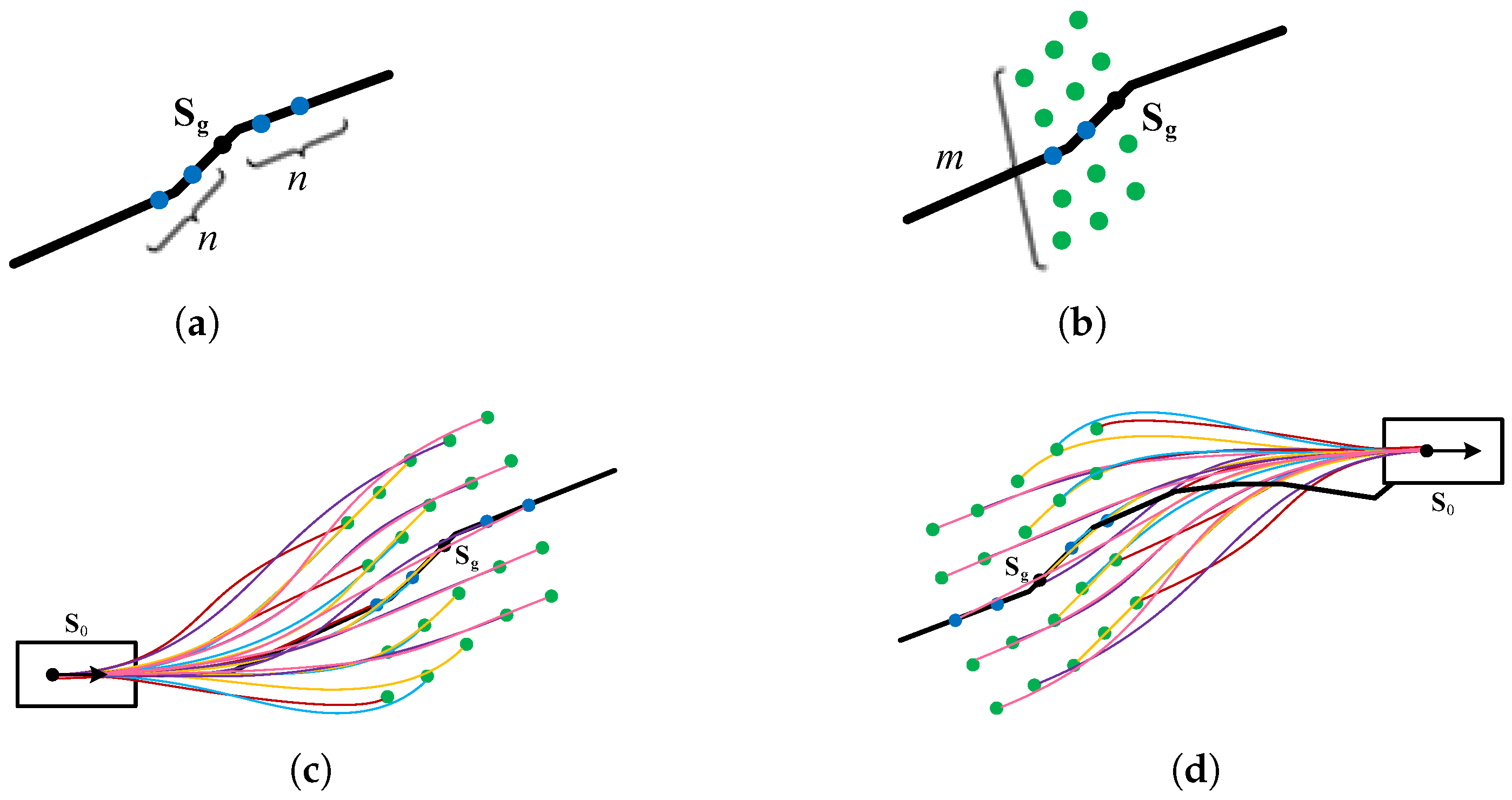
4.3.1. Method for Path Generation

Define $\mathbf{S}=(x,y,\theta ,\rho )$ as the state space of the vehicle, which includes position $(x,y)$, heading $\theta$, and path curvature $\rho$ at the current position. The problem of the path generation can be defined as follows: Given the start state ${\mathbf{S}}_0(x_0,y_0,{\theta }_0,{\rho }_0)$ and target state ${\mathbf{S}}_{\mathrm{g}}(x_{\mathrm{g}},y_{\mathrm{g}},{\theta }_{\mathrm{g}},{\rho }_{\mathrm{g}})$, search for a path that satisfies the nonholonomic constraints of the vehicle to connect ${\mathbf{S}}_0$ and ${\mathbf{S}}_{\mathrm{g}}$. Here, we focus on the curvature constraint by limiting the curvature of each segment of the path to the maximum curvature suitable for the vehicle.

To ensure the curvature continuity, we use a cubic polynomial spiral of the cumulative distance l to express the curvature of the path. The relationship between the vehicle state and the cumulative distance is

$$\left\{\begin{array}{c}x\left(l\right)=x_0+\int cos\theta \left(l\right)dl\hfill \\ y\left(l\right)=y_0+\int sin\theta \left(l\right)dl\hfill \\ \rho \left(l\right)={\rho }_0+a_{1}l+a_2{l}^2+a_3{l}^3\hfill \\ \theta \left(l\right)={\theta }_0+{\rho }_{0}l+a_1{\displaystyle \frac{l^2}{2}}+a_2{\displaystyle \frac{l^3}{3}}+a_3{\displaystyle \frac{l^4}{4}}\hfill \end{array}\right.$$

(11)

Additionally, minimizing the curvature can improve the safety of the vehicle in off-road environments. The path generation problem we define is as follows:

$$minf={\int }_0^{l_{\mathrm{g}}}\rho {\left(l\right)}^{2}dl={\int }_0^{l_{\mathrm{g}}}{({\rho }_0+a_{1}l+a_2{l}^2+a_3{l}^3)}^{2}dl,$$

$$\begin{array}{c}\mathrm{s}.\mathrm{t}.\left\{\begin{array}{c}\left|{\rho }_i\right|\le {\rho }_{max}(0\le i\le l_{\mathrm{g}})\hfill \\ S_{l=0}(x_0,y_0,{\theta }_0,{\rho }_0)\hfill \\ S_{l=l_{\mathrm{g}}}(x_{\mathrm{g}},y_{\mathrm{g}},{\theta }_{\mathrm{g}},{\rho }_{\mathrm{g}})\hfill \end{array},\right.\hfill \end{array}$$

(12)

where $l_{\mathrm{g}}$ is the length of the curve.

4.3.2. Optimal Local Path Evaluation

The local planner obtains the local path by generating several smooth paths and selecting the optimal one. As shown in Figure 3, we sample the smooth path based on the 2D projection of the global path. First, we select a reference position ${\mathbf{S}}_{\mathrm{g}}$ for sampling on the 2D path according to current speed of the vehicle. Second, the longitudinal layer samples n longitudinal points on either side of ${\mathbf{S}}_{\mathrm{g}}$ along the path. The lateral layer contains m sampling points based on each longitudinal sampling point. Third, we employ the path generation method mentioned in Section 4.3.1 to obtain the local path cluster (the total number is $(2n+1)\times m$), which smoothly connect the vehicle state with sample states. If the vehicle encounters a situation similar to the “dead end,” the selected target may be located behind the vehicle. It is important to note that in complex off-road environments with challenging terrain, the vehicle makes sharp turns can be dangerous, and the risk of accidents such as rollovers increases significantly. Additionally, it is difficult for the vehicle to make the turn in some confined spaces, which will affect exploration efficiency. Therefore, we consider planning reverse paths for the vehicle to avoid potential risks and improve exploration efficiency, as shown in Figure 3d.

Based on the requirements of exploration for vehicles in off-road environments, we construct an evaluation function in Equation (13) to obtain the optimal local path. ${\omega }_{\mathrm{S}}$ and ${\omega }_{\mathrm{T}}$ are the smoothness weight and traversability weight of the path, respectively. Their values determine their relative importance in the path selection process. $C_{\mathrm{S}}$ and $C_{\mathrm{T}}$ represent the evaluation value of the smoothness and traversability of the path.

$$f={\omega }_{\mathrm{S}}{C}_{\mathrm{S}}+{\omega }_{\mathrm{T}}{C}_{\mathrm{T}}$$

(13)

Define $\Gamma =\{x_1,x_2,\dots ,x_M\}$ as an evaluated path. The path smoothness $C_{\mathrm{S}}$ can be expressed as the mean of normalized curvature at each point on the $\Gamma$, as follows:

$$C_{\mathrm{S}}={\displaystyle \frac{1}{M}}{\sum }_{i=1}^M{\displaystyle \frac{\left|\rho \left(x_i\right)\right|}{{\rho }_{\max }}},$$

(14)

where $\rho \left(x_i\right)$ is the path curvature at $x_i$ and ${\rho }_{\max }$ is the maximum curvature suitable for the vehicle. The path traversability $C_{\mathrm{T}}$ can be calculated as the mean of the traversability cost at each point along the path.

$$C_{\mathrm{T}}={\displaystyle \frac{1}{M}}{\sum }_{i=1}^M\tau \left(x_i\right),$$

(15)

where $\tau \left(x_i\right)$ is the traversability cost at $x_i$. Lower $C_{\mathrm{S}}$ and $C_{\mathrm{T}}$ mean higher travel speed and safety for autonomous vehicles in complex off-road environments.

To enhance the efficiency of the feasibility analysis, we first evaluate all local paths in the cluster. Then, we conduct the feasibility analysis of paths in sequence based on their score, including checking for collisions and projecting onto the 3D surface. Once a feasible path is found, the feasibility analysis no longer continues, and the path is output to the vehicle as the optimal local path.

5. Experiments

5.1. Implementation Details

We conduct experiments in both simulation and real-world environments. Figure 4 shows the simulated wheeled vehicle model and the ground vehicle platform. In the simulation experiments, the simulation model is a four-wheel-drive differentially steered wheeled vehicle equipped with a 32-line lidar and the maximal speed is set to 0.8 m/s. The vehicle’s sensor range is set to 10 m. The exploration algorithm runs on a 2.2 GHz i7-8750 computer using a single CPU and employs the A-LOAM algorithm for environment mapping during the exploration. The map resolution for $ma{p}_{\mathrm{cloud}}$, $ma{p}_{\mathrm{state}}$, and $ma{p}_{\mathrm{trav}}$ is set to 0.1 m, 0.4 m, and 0.2 m, respectively; the max slope, roughness, and sparsity suitable for the vehicle is set to 25, 0.001, and 1.0, respectively; the step size of global and local RRT is 0.4 m and 0.8 m; the bandwidth used in the cluster is 1.0 m; and the total number of local path candidates is 55.

In the real-world experiments, our platform is equipped with sensors such as lidar, radar, and cameras. Additionally, the platform employs an autonomous driving software architecture that our team independently developed. Apart from replacing the vehicle’s decision-making and planning module with our proposed exploration algorithm, all other modules use the original software algorithm. The maximal speed is set to 15 km/h and the exploration algorithm runs on a 3.2 GHz i7-8700 computer using a single CPU.

The evaluation metrics for the vehicle’s exploration include the time and distance required to complete the exploration, as well as the traversability cost of its travel path. The exploration time and distance are determined by the duration and the distance the vehicle travels when each method meets its respective end conditions for exploration. The traversability cost of the vehicle’s travel path is calculated based on Equation (15). Considering the difficulty in estimating the volume of off-road environments, we manually supervise each exploration process. Exploration is considered failed in cases where the vehicle is involved in an accident, the exploration is not completed within a reasonable time, or it covers an insufficient area by the end of the exploration.

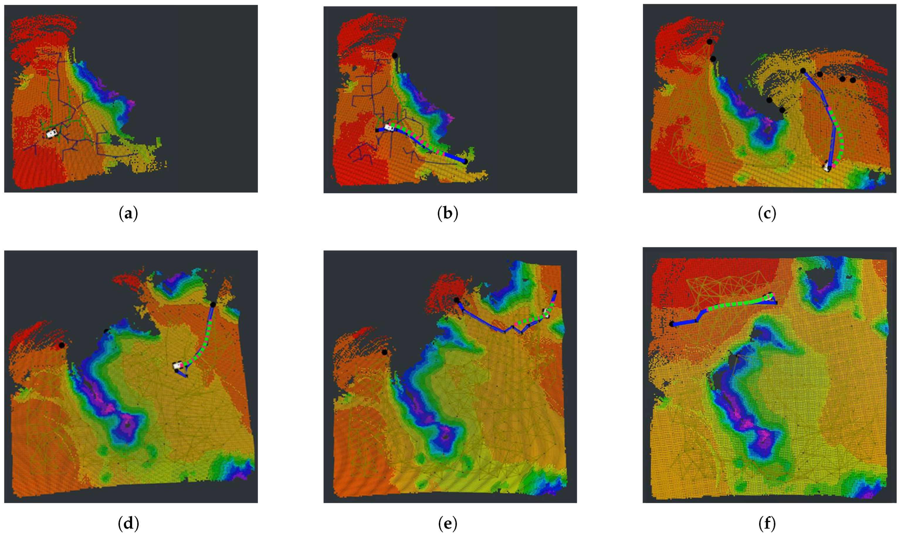
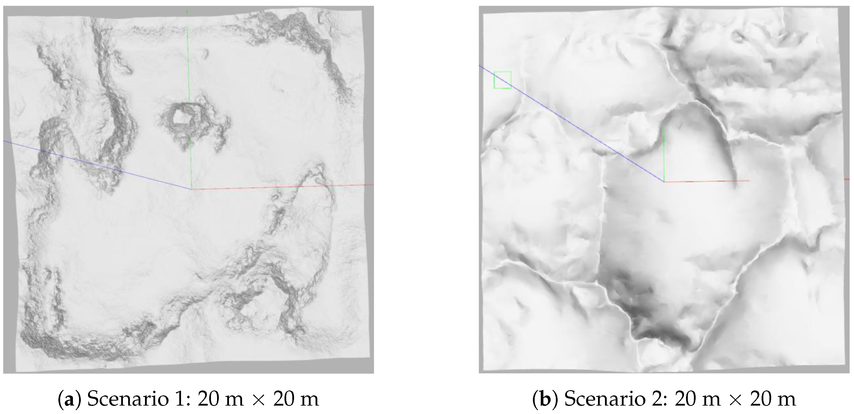
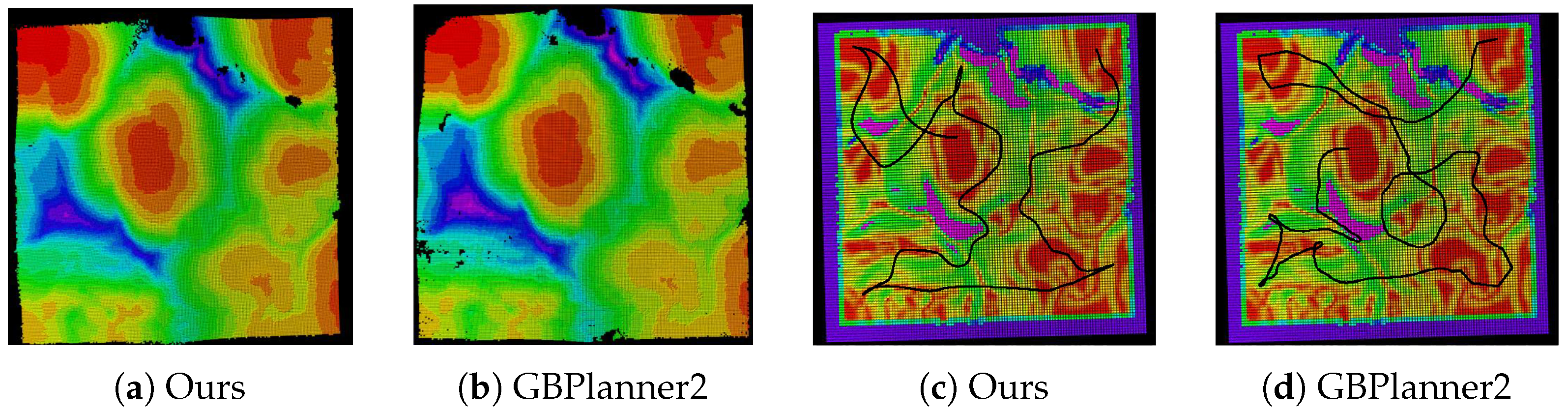
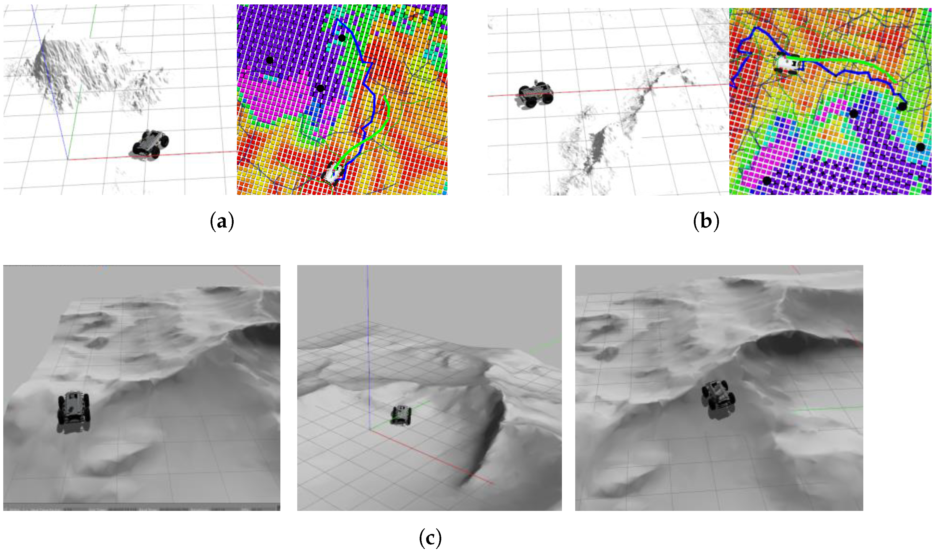
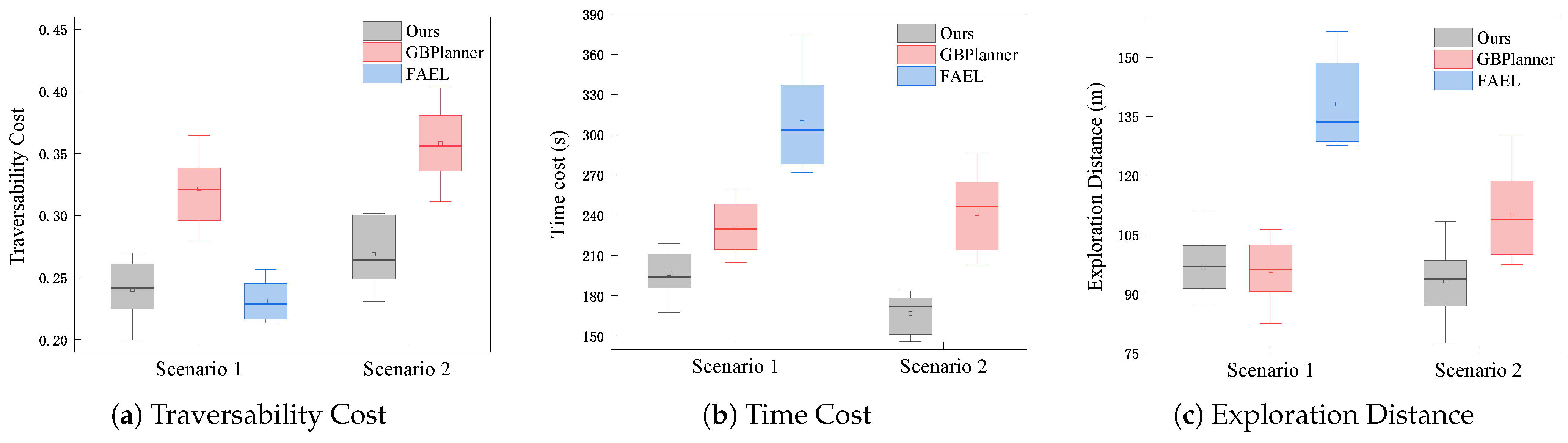
5.2. Simulation and Analysis

The illustration of the autonomous exploration process using our framework in a typical off-road simulation environment is shown in Figure 5. The vehicle detects the frontier at the start position (Figure 5a) using the global RRT (thin blue lines) and local RRT (thin green lines). Then, the detected frontier points are clustered to the candidate target points, which are shown as black points in the figure. In Figure 5b, the vehicle utilizes the 3D road map (tawny lines) to plan a global path (thick blue line). The thick green line in it represents the smoothed local path. Figure 5c–f show the construction process of the environmental map along with the exploration. As Figure 5 shows, our algorithm can provide a global path that avoids areas with poor traversability in the environment and a smooth and safe local path for the vehicle.

As shown in Figure 6, we verify our proposed method in two uneven simulation off-road scenarios to evaluate the performance of our framework. Scenario 1 is similar to the basin in that the central area is depressed and the bottom of the depression is littered with many protruding stones of varying sizes. Scenario 2 consists of numerous ridges and valleys, with some slopes having significantly steep gradients. These terrains pose great challenges for vehicles traversing through them. To ensure the vehicle’s safety and highlight the impact of rugged terrain on driving, we reduce the maximum speed limit of the vehicle when it encounters poor terrain conditions.

In order to investigate the performance from both quantitative and qualitative perspectives, we conduct multiple simulations in each simulation environment and make comparisons on the exploration result with GBPlanner2 (https://github.com/ntnu-arl/gbplanner_ros (accessed on 22 May 2025)) and FAEL [22]. GBPlanner2 is a revised and enhanced version of GBPlanner [23], which provides improved computational performance and better handling of positive and negative obstacles for ground robots. In the simulation experiments, our approach and GBPlanner2 complete the exploration tasks in both scenarios, while FAEL fails to complete the exploration in Scenario 2. Figure 7 and Figure 8 show the exploration result in the two simulation scenarios, respectively. Both the traversability grid map (the colors of map correspond to traversability cost variations) constructed by our algorithm, the corresponding exploration paths, and the resulting point cloud grid map (the colors of map correspond to height variations) are displayed in the figures. We observe that all methods demonstrate backtracking capabilities by finding new targets in global space after exploring local regions. However, compared with the other methods, our method generally returns smoother and safer exploration paths. GBPlanner2 follows the paths planned by Rapidly-exploring Random Graph (RRG), resulting in a more tortuous trajectory due to the lack of path smoothness, and the vehicle needs to stop frequently to adjust travel direction. FAEL tends to drive repeatedly in already explored areas, possibly due to the inapplicability of frontier detection, which increases the exploration distance and time. After reaching the current sub-goal, FAEL usually travels to the next subtarget by pivot steering. Our method considers the nonholonomic constraints of the vehicle in path planning and obtains smoother paths, which avoids stopping frequently. Additionally, the presence of “turn-back” regions in our exploration paths is due to our consideration of the vehicle’s ability to reverse when traveling to the next target. This consideration improves backtracking efficiency and avoids the risks of making large-angle steering in complex terrains.

Qualitatively speaking, as shown in Figure 7 and Figure 8, the traversability grid map constructed by our method essentially reflects the real terrain conditions of the simulation scenarios. It effectively marks areas that are difficult for the vehicle to traverse as untraversable areas (purple grids in figures). Moreover, we employ different resolutions for different grid layers, making the method retain fine details of the point cloud map while appropriately reducing the computational cost of traversability analysis. Additionally, our planning method demonstrates an outstanding ability to analyze terrain, and the paths obtained are more conducive to vehicle travel. On the one hand, our proposed method determines the traversable areas based on the vehicle’s dynamics. During the exploration, our method can timely abandon those areas untraversable for the vehicle or choose the appropriate route to detour. As shown in the red box in Figure 7a,d, GBPlanner2 and FAEL choose to return when encountering terrain with significant relative elevation. However, our approach identifies a more gentle slope to continue traversal according to the terrain analysis, thereby enabling exploration of more distant regions. It is worth noting that FAEL has never succeeded in the simulation experiments under Scenario 2. The main reason is that FAEL relies heavily on the point cloud map for terrain analysis. However, since the terrain in Scenario 2 consists almost entirely of areas with significant undulations, FAEL misclassified them as untraversable areas due to the elevation variations. As a result, the method fails to continue exploring the environment. On the other hand, benefiting from our traversability map, our method plans a path through areas where traversability cost is low, which avoids slowing down the vehicle and ensures safety, as shown in Figure 9. In Scenario 1, our method identifies that the protruding parts of the ground present a significant traversal challenge, so it prioritizes travel on the adjacent flat terrain. In Scenario 2, our method plans paths that keep the vehicle on relatively gentle slopes when passing over ridges, ensuring the safety and speed of vehicle travel.

Each simulation runs 10 times to provide quantitative evaluations. First, to verify the real-time performance of our environmental modeling method, we recorded the update times of each layer grid map during the exploration process.

Table 1. The average update times for multi-resolution layered grid map in simulation.

Environment	Point Cloud Map	Exploration State Map	Traversability Map
Scenario 1	12.658 ms	0.420 ms	34.718 ms
Scenario 2	10.807 ms	0.496 ms	32.411 ms

presents the average update times for each map in the two scenarios. As shown in the table, the map update times fully meet the real-time requirements for autonomous exploration in off-road environments. If $ma{p}_{\mathrm{trav}}$ and $ma{p}_{\mathrm{cloud}}$ have the same resolution, the computational time for traversability analysis would increase significantly, potentially compromising the vehicle’s navigation safety. Second, Figure 10 shows the statistics of the time and distance of exploration, and the traversability cost of the travel path in each scenario. As shown in the figure, our method demonstrates superior performance across all three evaluation metrics. FAEL achieves a relatively low traversability cost in Scenario 1 because it only explores areas with favorable terrain conditions and treats complex terrains directly as obstacles. However, since FAEL selects targets based solely on high-information regions, it often has to repeatedly explore between distant small areas, leading to higher time and distance costs. The corresponding average statistics are displayed in

Table 2. The average statistics of exploration in simulation.

Environment	Method	Time (s)	Distance (m)	Average Speed (m/s)	Traversability Cost
	ours	196.306	97.103	0.495	0.240298
Scenario 1	GBPlanner2	230.780 (14.94%)	95.911 (−1.24%)	0.416	0.321456 (25.25%)
	FAEL	309.219 (36.52%)	138.153 (29.71%)	0.457	0.231264 (−3.91%)
	ours	166.756	93.203	0.559	0.268938
Scenario 2	GBPlanner2	241.095 (30.83%)	110.059 (15.32%)	0.456	0.358106 (24.90%)
	FAEL	-	-	-	-

The numbers in ( ) indicate the performance improvement of our method compared with the comparative methods in terms of the corresponding metrics.

. The results show that our method can achieve a maximum improvement of 36.52% in terms of time cost and up to 25.25% improvement in traversability cost compared to the baseline methods. We also observe that the vehicle using our method has a higher average speed than using other methods. The reason for this is that paths planned by our method have better traversability, which ensures the travel speed of the vehicle.

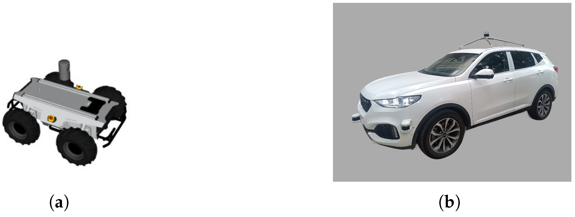
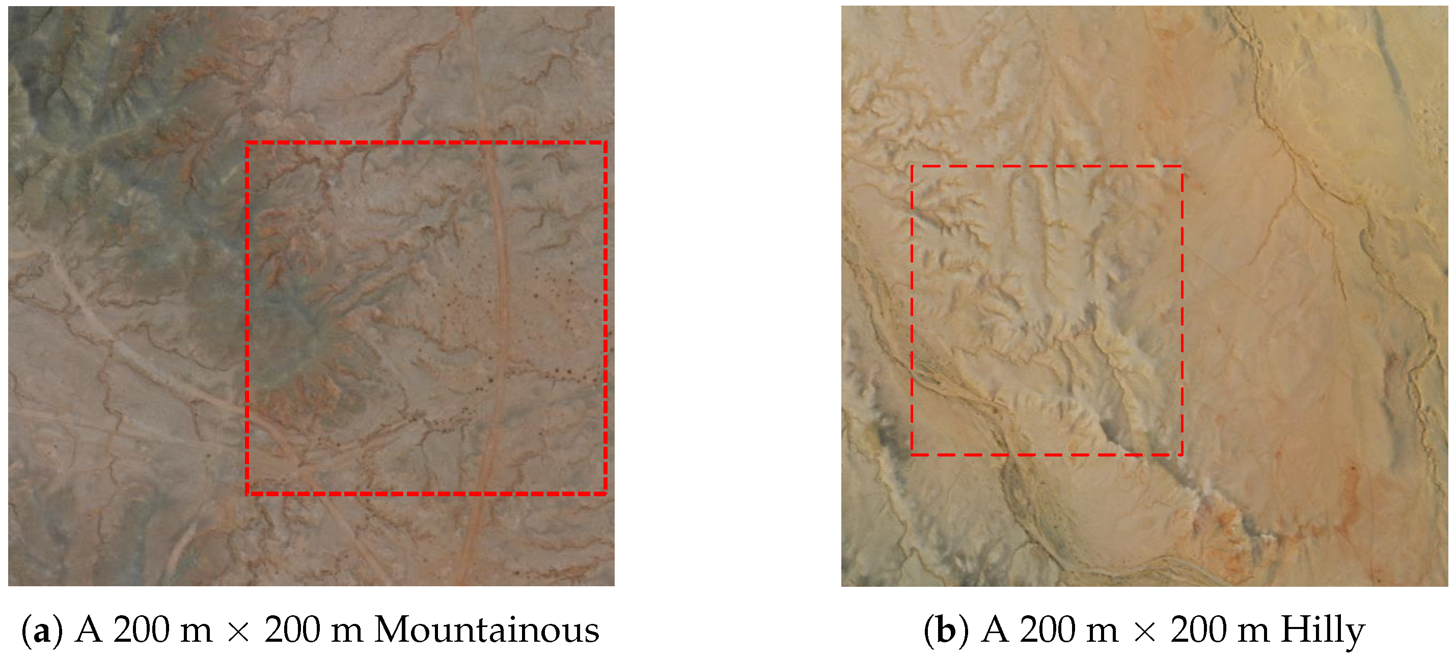
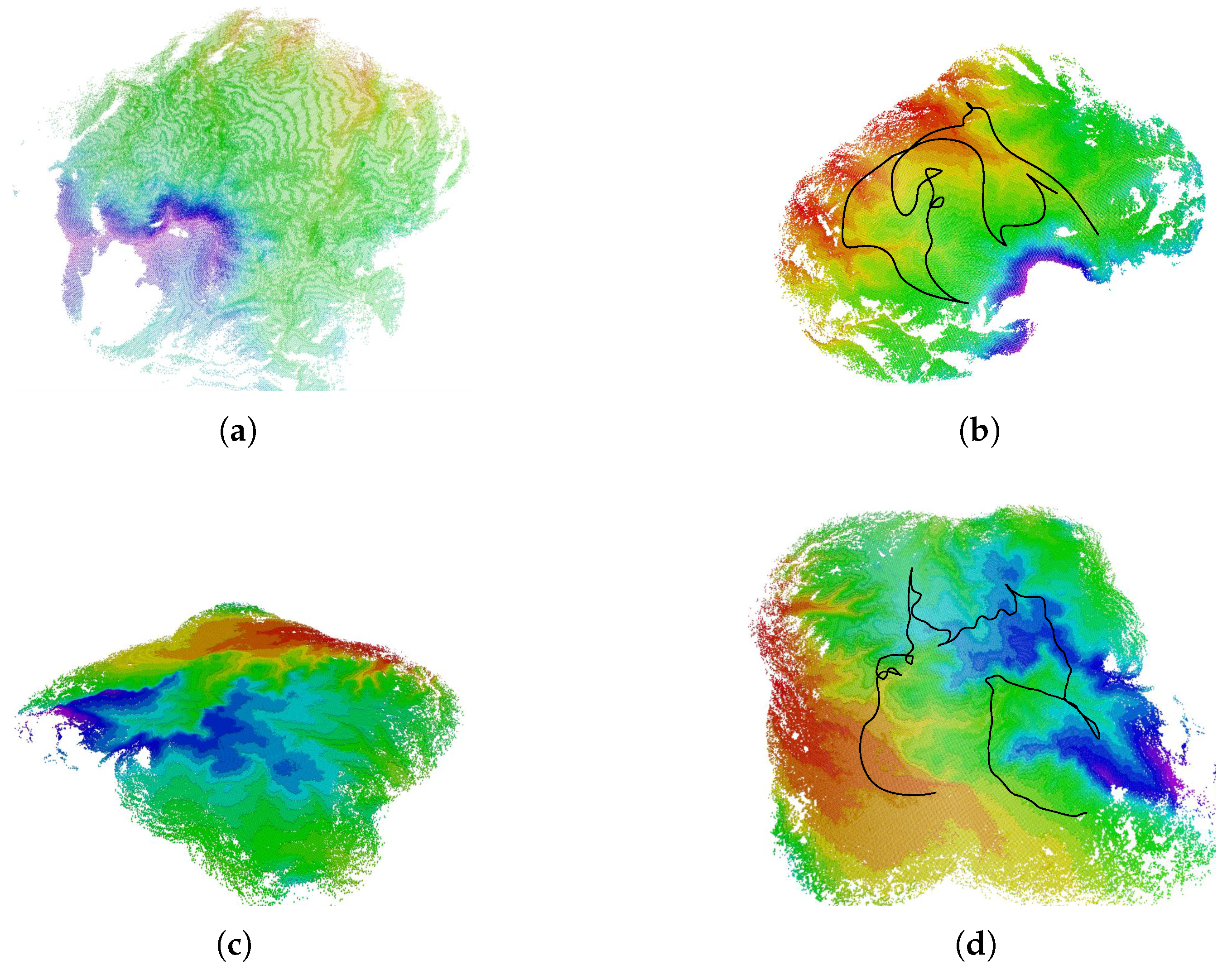
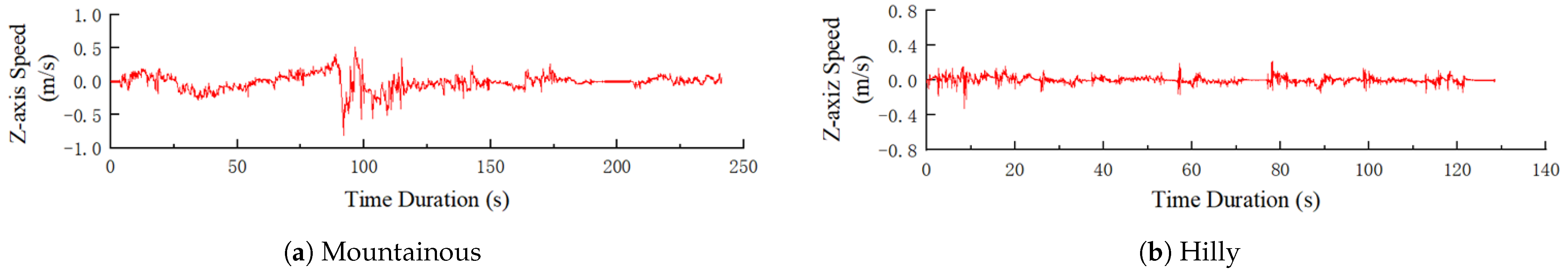
5.3. Real-World Tests

To further validate the proposed method, we use the ground vehicle to explore a mountainous region and a hilly region in real-world experiments, as shown in Figure 11a,b. The mountainous terrain, as a typical off-road scenario, is characterized by rugged surfaces and continuous undulating sections, which can significantly impact the stability of vehicle travel. Compared with mountainous areas, the hilly terrain is less steep, allowing vehicles to travel. However, the continuous slopes can still affect the vehicle’s travel speed. The results for these scenarios are displayed in Figure 12. The time and distance for exploration, along with the traversability cost of the travel path, are displayed in

Table 3. The statistics for exploration in the real world.

Environment	Time	Distance	Average Speed	Traversability Cost
Mountainous	243.32 s	570.021 m	2.342 m/s	0.289153
Hilly	182.69 s	500.125 m	2.737 m/s	0.269926

. In the mountainous region, we can observe that the vehicle avoids exploring the mountaintop and chooses to travel flat regions. In the hilly region, the vehicle explores the ridge from some relatively gentle slopes. The Z-axis speed variations of the vehicle during the exploration are presented in Figure 13. By analyzing the change in vertical speed of the vehicle and the traversability cost of the travel path, the framework shows the complete exploration of the environments with a reasonable exploration path in both cases, demonstrating the practical feasibility of our framework.

The comprehensive analysis of the experimental results demonstrates the safety and efficiency of our algorithm and indicates that our exploration algorithm is suitable for complex off-road environments. Our framework ensures that vehicles can explore unknown off-road terrains at faster speeds. However, due to the uncertainty localization and perception data in real-world scenarios, there can be discrepancies between the constructed environmental maps and the actual scenarios. To ensure the vehicle’s travel safety, we utilize the current frame’s point cloud data and historical point cloud data to jointly estimate the traversability cost, preventing the vehicle from making incorrect terrain assessments.

6. Conclusions

We propose a method of path planning for autonomous exploration that is suitable for autonomous vehicles in off-road environments. Our method constructs a multi-resolution layered grid environmental model by analyzing the traversability of the environment. Based on this model, the path planning for exploration is conducted in two steps. In the first step, we extend the RRT frontier detector from 2D to 3D to capture frontier variations in off-road environments. Then, the traversability cost is incorporated as a key reference for frontier clustering and target selection, ensuring that the selected targets are accessible to the vehicle. In the second step, we select the optimal local path from the path cluster based on the global path to improve the smoothness and traversability of the local path. Both simulations and real-world experiments show the effectiveness of our method.

The limitation of our method is the randomness inherent in RRTs, which affects the timely response to environmental changes. In the future, we plan to develop more promising heuristics to help with the sampling for frontier detection and consider multi-vehicle 3D exploration to further enhance the exploration efficiency.

References

1. Zhang, X.; Wang, J.; Wang, S.; Wang, M.; Wang, T.; Feng, Z.; Zhu, S.; Zheng, E. FAEM: Fast Autonomous Exploration for UAV in Large-Scale Unknown Environments Using LiDAR-Based Mapping. Drones 2025, 9, 423. [Google Scholar] [CrossRef]
2. Qi, C.; Ma, T.; Li, Y.; Ling, Y.; Liao, Y.; Jiang, Y. A Multi-AUV Collaborative Mapping System with Bathymetric Cooperative Active SLAM Algorithm. IEEE Internet Things J. 2025, 12, 12441–12452. [Google Scholar] [CrossRef]
3. Zhou, Z.; Chen, Y.; Yu, J.; Zu, B.; Wang, Q.; Zhou, X.; Duan, J. Mars Exploration: Research on Goal-Driven Hierarchical DQN Autonomous Scene Exploration Algorithm. Aerospace 2024, 11, 692. [Google Scholar] [CrossRef]
4. Niroui, F.; Zhang, K.; Kashino, Z.; Nejat, G. Deep Reinforcement Learning Robot for Search and Rescue Applications: Exploration in Unknown Cluttered Environments. IEEE Robot. Autom. Lett. 2019, 4, 610–617. [Google Scholar] [CrossRef]
5. Cao, Z.; Du, Z.; Yang, J. Topological Map-Based Autonomous Exploration in Large-Scale Scenes for Unmanned Vehicles. Drones 2024, 8, 124. [Google Scholar] [CrossRef]
6. Wang, K.; Wang, M.; Wang, R.; Zhai, C.; Song, W. Traversability Estimation for Off-Road Autonomous Driving Under Ego-Motion Uncertainty. IEEE Sens. J. 2024, 24, 6584–6596. [Google Scholar] [CrossRef]
7. Jiang, J.; Hu, Z.; Xie, Z.; Hao, C.; Liu, H.; Xu, W.; Kong, Z.; Wang, Y.; He, L.; Xu, S.; et al. A Risk-Aware Planning Framework of UGVs in Off-Road Environment. IEEE Trans. Veh. Technol. 2025, 74, 3870–3884. [Google Scholar] [CrossRef]
8. Chen, Y.; Wang, R.; Qu, Y.; Yan, C.; Song, W. GRRL: Goal-Guided Risk-Inspired Reinforcement Learning for Efficient Autonomous Driving in Off-Road Environment. In Proceedings of the 2024 China Automation Congress (CAC), Qingdao, China, 1–3 November 2024; pp. 2496–2501. [Google Scholar] [CrossRef]
9. Lee, J.; Kurisu, M.; Kuriyama, K. Three-dimensionalized feature-based LiDAR-visual odometry for online mapping of unpaved road surfaces. J. Field Robot. 2024, 41, 1452–1468. [Google Scholar] [CrossRef]
10. Umari, H.; Mukhopadhyay, S. Autonomous robotic exploration based on multiple rapidly-exploring randomized trees. In Proceedings of the IEEE/RSJ International Conference on Intelligent Robots and Systems (IROS), Vancouver, BC, Canada, 24–28 September 2017; pp. 1396–1402. [Google Scholar] [CrossRef]
11. Ahmed, M.F.; Masood, K.; Fremont, V.; Fantoni, I. Active SLAM: A Review on Last Decade. Sensors 2023, 23, 8097. [Google Scholar] [CrossRef]
12. Cao, Y.; Zhao, R.; Wang, Y.; Xiang, B.; Sartoretti, G. Deep Reinforcement Learning-Based Large-Scale Robot Exploration. IEEE Robot. Autom. Lett. 2024, 9, 4631–4638. [Google Scholar] [CrossRef]
13. Huang, J.; Fan, Z.; Yan, Z.; Duan, P.; Mei, R.; Cheng, H. Efficient UAV Exploration for Large-Scale 3D Environments Using Low-Memory Map. Drones 2024, 8, 443. [Google Scholar] [CrossRef]
14. Liu, J.; Lv, Y.; Yuan, Y.; Chi, W.; Chen, G.; Sun, L. An Efficient Robot Exploration Method Based on Heuristics Biased Sampling. IEEE Trans. Ind. Electron. 2023, 70, 7102–7112. [Google Scholar] [CrossRef]
15. Respall, V.M.; Devitt, D.; Fedorenko, R.; Klimchik, A. Fast Sampling-based Next-Best-View Exploration Algorithm for a MAV. In Proceedings of the IEEE International Conference on Robotics and Automation (ICRA), Xi’an, China, 30 May–5 June 2021; pp. 89–95. [Google Scholar] [CrossRef]
16. Yu, J.; Shen, H.; Xu, J.; Zhang, T. ECHO: An Efficient Heuristic Viewpoint Determination Method on Frontier-Based Autonomous Exploration for Quadrotors. IEEE Robot. Autom. Lett. 2023, 8, 5047–5054. [Google Scholar] [CrossRef]
17. Dang, T.; Papachristos, C.; Alexis, K. Visual Saliency-Aware Receding Horizon Autonomous Exploration with Application to Aerial Robotics. In Proceedings of the International Conference on Robotics and Automation (ICRA), Brisbane, QLD, Australia, 21–25 May 2018; pp. 2526–2533. [Google Scholar] [CrossRef]
18. Batinovic, A.; Petrovic, T.; Ivanovic, A.; Petric, F.; Bogdan, S. A Multi-Resolution Frontier-Based Planner for Autonomous 3D Exploration. IEEE Robot. Autom. Lett. 2021, 6, 4528–4535. [Google Scholar] [CrossRef]
19. Zhou, B.; Zhang, Y.; Chen, X.; Shen, S. FUEL: Fast UAV Exploration Using Incremental Frontier Structure and Hierarchical Planning. IEEE Robot. Autom. Lett. 2021, 6, 779–786. [Google Scholar] [CrossRef]
20. Duberg, D.; Jensfelt, P. UFOExplorer: Fast and Scalable Sampling-Based Exploration with a Graph-Based Planning Structure. IEEE Robot. Autom. Lett. 2022, 7, 2487–2494. [Google Scholar] [CrossRef]
21. Cao, C.; Zhu, H.; Choset, H.; Zhang, J. TARE: A Hierarchical Framework for Efficiently Exploring Complex 3D Environments. In Proceedings of the Robotics: Science and Systems, Virtually, 12–16 July 2021. [Google Scholar] [CrossRef]
22. Huang, J.; Zhou, B.; Fan, Z.; Zhu, Y.; Jie, Y.; Li, L.; Cheng, H. FAEL: Fast Autonomous Exploration for Large-scale Environments With a Mobile Robot. IEEE Robot. Autom. Lett. 2023, 8, 1667–1674. [Google Scholar] [CrossRef]
23. Dang, T.; Tranzatto, M.; Khattak, S.; Mascarich, F.; Alexis, K.; Hutter, M. Graph-based subterranean exploration path planning using aerial and legged robots. J. Field Robot 2020, 37, 1363–1388. [Google Scholar] [CrossRef]
24. Zhu, H.; Cao, C.; Xia, Y.; Scherer, S.; Zhang, J.; Wang, W. DSVP: Dual-Stage Viewpoint Planner for Rapid Exploration by Dynamic Expansion. In Proceedings of the IEEE/RSJ International Conference on Intelligent Robots and Systems (IROS), Prague, Czech Republic, 27 September–1 October 2021; pp. 7623–7630. [Google Scholar] [CrossRef]
25. Chen, X.; Zheng, J.; Hu, Q. A Hybrid Planning Method for 3D Autonomous Exploration in Unknown Environments with a UAV. IEEE Trans. Autom. Sci. Eng. 2024, 21, 5713–5724. [Google Scholar] [CrossRef]
26. Li, Y.; Debnath, A.; Stein, G.J.; Košecká, J. Learning-Augmented Model-Based Planning for Visual Exploration. In Proceedings of the IEEE/RSJ International Conference on Intelligent Robots and Systems (IROS), Detroit, MI, USA, 1–5 October 2023; pp. 5165–5171. [Google Scholar] [CrossRef]
27. Tang, Y.; Cai, J.; Chen, M.; Yan, X.; Xie, Y. An autonomous exploration algorithm using environment-robot interacted traversability analysis. In Proceedings of the 2019 IEEE/RSJ International Conference on Intelligent Robots and Systems (IROS), Macau, China, 3–8 November 2019; pp. 4885–4890. [Google Scholar] [CrossRef]
28. Jian, Z.; Lu, Z.; Zhou, X.; Lan, B.; Xiao, A.; Wang, X.; Liang, B. PUTN: A Plane-fitting based Uneven Terrain Navigation Framework. In Proceedings of the IEEE/RSJ nternational Conference on Intelligent Robots and Systems (IROS), Kyoto, Japan, 23–27 October 2022; pp. 7160–7166. [Google Scholar] [CrossRef]
29. Tang, J.; Jiang, F.; Long, Y.; Fu, L.; Sun, H. Identification of the yield of camellia oleifera based on color space by the optimized mean shift clustering algorithm using terrestrial laser scanning. Remote Sens. 2022, 14, 642. [Google Scholar] [CrossRef]
30. Wang, C.; Chi, W.; Sun, Y.; Meng, M.Q.H. Autonomous Robotic Exploration by Incremental Road Map Construction. IEEE Trans. Autom. Sci. Eng. 2019, 16, 1720–1731. [Google Scholar] [CrossRef]
31. Qi, Y.; He, B.; Wang, R.; Wang, L.; Xu, Y. Hierarchical Motion Planning for Autonomous Vehicles in Unstructured Dynamic Environments. IEEE Robot. Autom. Lett. 2023, 8, 496–503. [Google Scholar] [CrossRef]
Figure 1. An overview of the proposed exploration framework. The vehicle senses the surrounding environment, and then the SLAM module uses the sensor data to output a global map. Based on the global map, we construct a multi-resolution layered grid map to provide environmental information for exploration. Next, the target selection module uses two RRTs to detect the frontier and obtain an accessible target and a corresponding global path. The global path is imported to the local planning module, which samples target states and generates a local path cluster. The optimal local path is then input into the vehicle.
Drones 09 00490 g001
Figure 2. Illustration of construction for the multi-resolution layered grid map. In the left multi-resolution layered grid map, the layers are ordered from top to bottom as m a p cloud , m a p trav , and m a p state . In m a p cloud , the red grid represents low elevation, and the purple grid represents high elevation. In m a p trav , the red grid represents low traversability cost, and the purple grid represents high traversability cost.
Drones 09 00490 g002
Figure 3. Local path sampling based on the global path. (a) Longitudinal sampling. (b) Lateral sampling. (c) The local path cluster obtained by sampling. (d) Planning reverse paths for the vehicle.
Drones 09 00490 g003
Figure 4. (a) Simulated wheeled vehicle (0.93 m × 0.70 m × 0.35 m) and (b) ground vehicle platform (4.6 m × 2.2 m × 2.4 m).
Drones 09 00490 g004
Figure 5. Autonomous exploration using our proposed framework in typical off-road environments. The point cloud map m a p cloud expands incrementally as the vehicle moves. (a) Thin blue lines are the global RRT and thin green lines are the local RRT. (bf) Black dots are candidate target points. Tawny lines consit of the 3D road map. Thick blue line is the global path. Thick green line is the local path.
Drones 09 00490 g005
Figure 6. Two off-road environments for simulation experiments.
Drones 09 00490 g006
Figure 7. Exploration results for Scenario 1. (ac) The resulting point cloud map of the scenario (resolution = 0.1 m). (df) Our traversability grid map and the exploration paths (black lines) of three methods.
Drones 09 00490 g007
Figure 8. Exploration results for Scenario 2. (a,b) The resulting point cloud map of the scenario (resolution = 0.1 m). (c,d) Our traversability grid map and the exploration paths (black lines) of two methods.
Drones 09 00490 g008
Figure 9. Illustration of the exploration paths planned by our method. (a,b) In Scenario 1, our method generates a path that avoids areas with poor traversability. (c) In Scenario 2, our method selects a path that travels through relatively flat terrain.
Drones 09 00490 g009
Figure 10. Statistics of exploration in simulation environments. (a) Traversability cost of the travel path. (b) Exploration time. (c) Exploration distance.
Drones 09 00490 g010
Figure 11. Two off-road environments for real-world experiments.
Drones 09 00490 g011
Figure 12. Exploration results for real environments. (a,b) The map and exploration path in the mountainous region. (c,d) The map and exploration path in the hilly region.
Drones 09 00490 g012
Figure 13. The Z-axis speed variations of the vehicle during the exploration.
Drones 09 00490 g013