Drone State Estimation Based on Frame-to-Frame Template Matching with Optimal Windows

Abstract

The flight capability of drones expands the surveillance area and allows drones to be mobile platforms. Therefore, it is important to estimate the kinematic state of drones. In this paper, the kinematic state of a mini drone in flight is estimated based on the video captured by its camera. A novel frame-to-frame template-matching technique is proposed. The instantaneous velocity of the drone is measured through image-to-position conversion and frame-to-frame template matching using optimal windows. Multiple templates are defined by their corresponding windows in a frame. The size and location of the windows are obtained by minimizing the sum of the least square errors between the piecewise linear regression model and the nonlinear image-to-position conversion function. The displacement between two consecutive frames is obtained via frame-to-frame template matching that minimizes the sum of normalized squared differences. The kinematic state of the drone is estimated by a Kalman filter based on the velocity computed from the displacement. The Kalman filter is augmented to simultaneously estimate the state and velocity bias of the drone. For faster processing, a zero-order hold scheme is adopted to reuse the measurement. In the experiments, two 150 m long roadways were tested; one road is in an urban environment and the other in a suburban environment. A mini drone starts from a hovering state, reaches top speed, and then continues to fly at a nearly constant speed. The drone captures video 10 times on each road from a height of 40 m at a 60-degree camera tilt angle. It will be shown that the proposed method achieves average distance errors at low meter levels after the flight.

1. Introduction

Drones can hover or fly while capturing videos from a distance. They can cover large and remote areas. They can conduct surveillance from various viewpoints and altitudes [1,2,3]. They are also cost-effective and do not require highly trained personnel [4]. Flying drones also act as mobile sensing platforms; drones are equipped with various sensors to collect data during flight [5,6]. Therefore, the position and velocity information of drones are essential for navigation, surveillance, and other high-level tasks. For example, drones can follow predefined trajectories, track multiple targets, and optimize formation in swarm operations.

A drone’s location is typically estimated using a combination of external sensors such as global positioning system (GPS) and internal sensors such as inertial measurement units (IMUs). GPS provides absolute position information but is vulnerable to external conditions [7,8]. In GPS-denied environments, reliable localization and state estimation remain critical challenges. Visual–inertial odometry systems that fuse data from IMUs and cameras are among the prominent solutions [9,10]. Although IMUs provide fast updates and require no external infrastructure, their estimation performance degrades over time due to drift errors [8]. Drone localization methods using LiDAR or depth cameras have been developed, providing high-precision spatial perception independent of visual texture or illuminations [11,12]. However, their use is generally limited to low altitudes or indoor environments [13,14,15,16]. Radio frequency (RF)-based localization methods use ultra-wideband (UWB) or other radio signals. They often require pre-installed infrastructure and careful calibration [17].

Approaches based solely on visual data from cameras are lightweight, cost-effective, and energy-efficient, while avoiding the complexity of sensor fusion. Vision-based localization techniques often rely on object template or feature matching across images [18]. Frame-to-frame template matching is commonly used to estimate displacement between consecutive frames [19]. It can track motion by matching a template from the previous frame to the current frame. Standard template matching works well for small displacements in environments without lighting, rotation, or scale changes [20]. A template is a region of interest (ROI) selected from a fixed area or object in the first frame or a reference image. Template selection may depend on terrain, objects, or explicit features [18,21]. Moving foreground regions were used as automatic template candidates with Gaussian mixture modeling of the background [22]. Photometric property-based template selection was developed to choose templates depending on the intensity, contrast, or gradient of pixels [21,23]. Selecting a proper template is critical for accurate motion estimation. As scenes or objects change over time, templates need to be updated, but incorrect updates can lead to accumulated errors that degrade performance [24].

In this paper, the kinematic state of a drone in flight is estimated only from frames captured by its camera. Frame-to-frame template matching using optimal windows is proposed to compute the instantaneous velocity of the drone. The optimal window divides the frame into several non-overlapping regions where the non-uniform spacing of the real coordinates is minimized.

Imaging projects 3D space onto a 2D plane, and this projection can be modeled using principles of ray optics [25]. The image-to-position conversion converts the discrete coordinates of pixels into continuous real-world coordinates [26]. During the conversion, the image size, the camera’s horizontal and vertical angular field of view (AFOV), elevation, and tilt angle are assumed to be known. However, this conversion process generates non-uniform spacing in real-world coordinates. When the camera points straight down, the pixel spacing is the most uniform. In [27], an entire frame is set as a template to estimate the drone’s speed from the vertical view. However, the spatial and visual information is one-sided, and the surveillance area becomes narrower in the vertical view. The optimal windows are contrived to overcome the non-uniform spacing distortion in the real-world coordinates. The height and location of the optimal windows are obtained from the piecewise linear segments that best fit the image-to-position conversion function in the vertical direction. The split points of the line segments are determined so as to minimize the sum of least square errors of the separate linear regression lines [28,29]. Therefore, multiple templates defined by the optimal windows are independent of the scene and object. No additional process is required for the template update. The matching of each template is performed by minimizing the sum of normalized squared differences [30], and the instantaneous velocity is measured from the average displacement obtained through multiple template matching.

The drone’s kinematic state is estimated based on the measured velocity using a Kalman filter, which adopts a nearly constant acceleration (NCA) model [31]. The state of the Kalman filter is augmented to simultaneously estimate the drone’s state and bias in velocity [32]. Since the computational complexity of frame matching is high, an augmented-state Kalman filter with a zero-order hold scheme [33] is adopted for faster processing. The zero-order hold Kalman filter reuses the measurement until new measurements are available.

Figure 1 shows a block diagram of the proposed method. First, the drone’s velocity is measured by image-to-position conversion and frame-to-frame template matching using optimal windows. The instantaneous velocity calculated by the frame-to-frame template matching is input into the Kalman filter as the measurement value. Next, the drone’s state and bias in the velocity are estimated through the augmented Kalman filter.

In the experiment, a mini drone weighing less than 250 g [34] flies along two approximately 150 m long roads and captures video at 30 frame per second (FPS). One road is an urban environment, and the other is a suburban environment. The drone starts from a stationary hovering position, accelerates to maximum speed, and continues to fly at a nearly constant speed at an altitude of 40 m and a camera tilt angle of 60 degrees. The frame size is 3840 × 2160 pixels, and the AFOV of the camera is assumed to be 64 and 40 degrees in horizontal and vertical directions, respectively. Ten flights were repeated on each road under various traffic conditions. For faster processing, four additional frame-matching speeds (10, 3, 1, 0.5 FPS) were tested using the zero-order hold Kalman filter. The proposed method is shown to achieve the average flight distance errors of 3.07–3.52 m and 1.97–2.39 m for Roads 1 and 2, respectively.

The contributions of this study are as follows: (1) Multiple template selection using optimal windows is proposed. The optimal windows are determined only by the image size, the camera’s AFOV, elevation, and tilt angle. Therefore, the template selection process is independent of the scene or object. (2) The augmented-state Kalman filter is designed to improve the accuracy of the drone’s state. The drone’s flight distance can be estimated with high accuracy, resulting in low-meter-level average errors. (3) Real-time processing is possible with the zero-order hold Kalman filter. This method maintains similar error levels even when the frame-matching speed is reduced to 0.5 FPS.

The rest of this paper is organized as follows: The real-world conversion and frame-to-frame template matching with optimal windows are described in Section 2. Section 3 explains drone state estimation with the augmented-state Kalman filter. Section 4 presents experimental results. Discussion and conclusions follow in Section 5 and Section 6, respectively.

2. Vision-Based Drone Velocity Computation

This section describes how the instantaneous velocity is measured by a combination of image-to-position conversion and frame-to-frame template matching based on optimal windows.

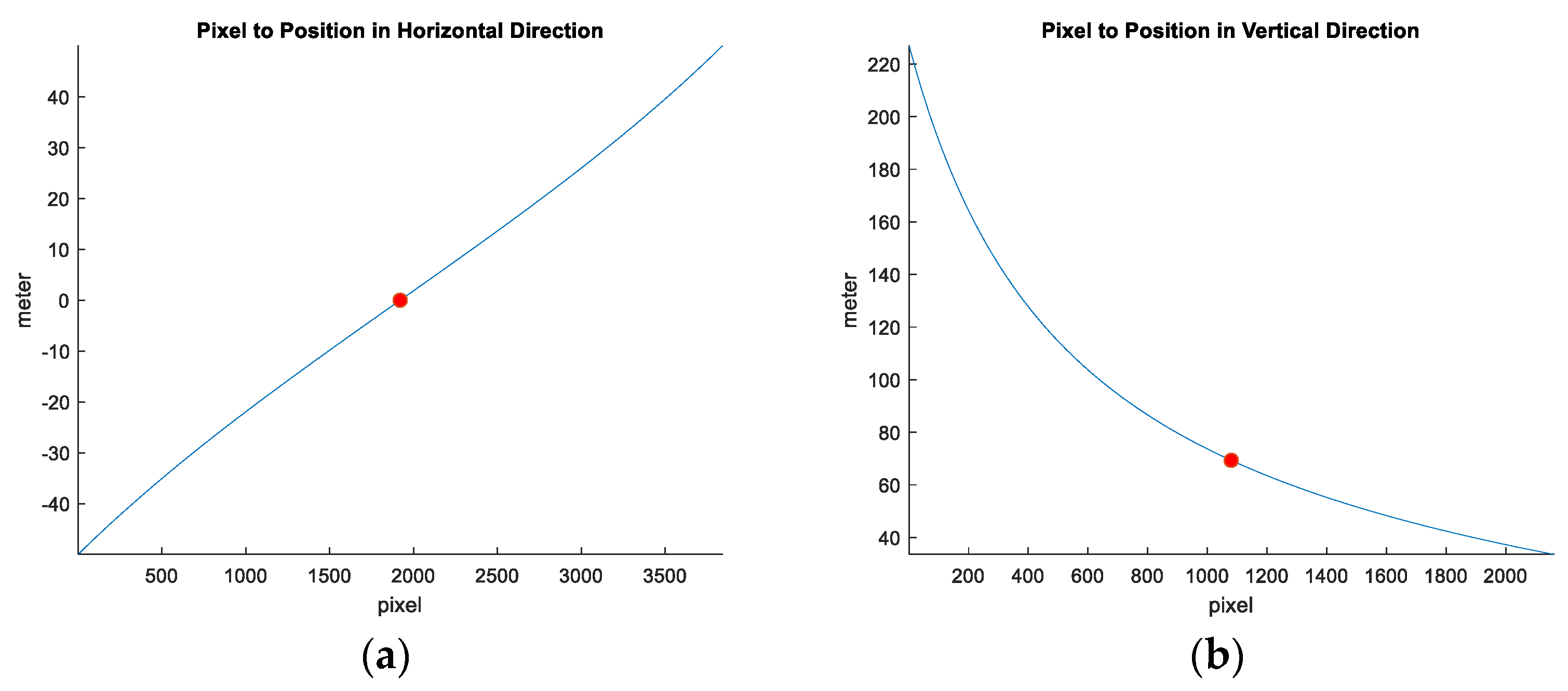
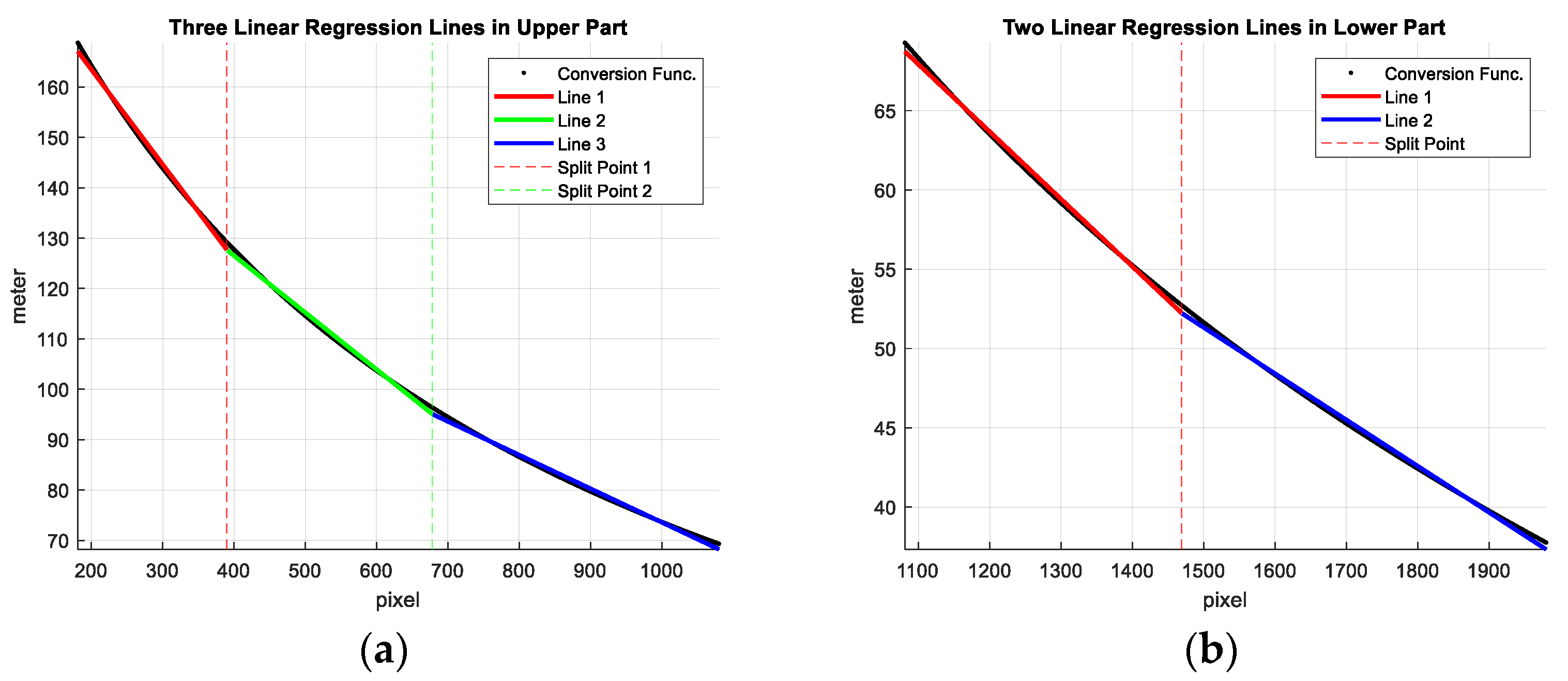
2.1. Image-to-Position Conversion

The image-to-position conversion [26] applies trigonometry to compute real-world coordinates from image pixel coordinates when the camera’s AFOV, elevation, and tilt angles are known. It is assumed that the camera rotates only around the pitch axis and that the ground is flat. It provides a simple and direct conversion from pixel coordinates to real-world coordinates. However, the non-uniform spacing in the real-world coordinates becomes a factor as the tilt angle increases. The real-world position vector $\left(x_i,y_j\right)$ corresponding to the (i, j) pixel is calculated as follows [26]:

$$\begin{gathered} \left(x_i,y_j\right)=\left(d_{{\displaystyle \frac{H}{2}}}·tan\left[\left(i-{\displaystyle \frac{W}{2}}+1\right){\displaystyle \frac{a_x}{W}}\right], h ·tan\left[{\theta }_T+\left({\displaystyle \frac{H}{2}}-j\right){\displaystyle \frac{a_y}{H}}\right]\right), \\ i=0,\dots ,W-1, j=0,\dots ,H-1, \end{gathered}$$

(1)

where W and H are the image sizes in the horizontal and vertical directions, respectively, h is the altitude of the drone or the elevation of the camera, $a_x$ and $a_y$ are the camera AFOV in the horizontal and vertical directions, respectively, and ${\theta }_T$ is the tilt angle of the camera; $d_{H/2}$ is the distance from the camera to ($x_{W/2-1}$, $y_{H/2}$,0), which is $h·\sec \left({\theta }_T\right)$. Figure 2 illustrates the coordinate conversion from image to real world [26].

Figure 3 visualizes the coordinate conversion function in horizontal and vertical directions according to Equation (1): W and H are set to 3840 and 2160 pixels, respectively; $a_x$ and $a_y$ are set to 64° and 40°, respectively; h is set to 40 m; ${\theta }_T$ is set to 60°. The nonlinearity increases rapidly as pixels move away from the center, resulting in non-uniform spacing in real-world coordinates, especially in Figure 3b. This distortion should be remedied when calculating the actual displacement in the image. In the next subsection, we will see how to overcome these distortions using optimal windows.

2.2. Frame-to-Frame Template Matching Based on Optimal Windows

The instantaneous velocity is computed at k frame as follows:

$${\mathit{z}}_{\mathit{m}}\left(k\right)=\left[\begin{array}{c}{z}_{mx}\left(k\right)\\ z_{my}\left(k\right)\end{array}\right]={\displaystyle \frac{1}{T}}{\displaystyle \frac{1}{N_w}}{\sum }_{n=1}^{N_w}\left[{{\mathit{c}}_n-\mathit{p}}_n\left(k\right)\right],$$

(2)

$${\mathit{c}}_{\mathit{n}}=img2pos\left\{\left[\begin{array}{c}{c}_{nx}\\ c_{ny}\end{array}\right]\right\},$$

(3)

$${\mathit{p}}_{\mathit{n}}\left(k\right)=img2pos\left\{\left[\begin{array}{c}{p}_{nx}\left(k\right)+c_{nx}\\ p_{ny}\left(k\right)+c_{ny}\end{array}\right]\right\},$$

(4)

where T is the sampling time between two consecutive frames, $N_w$ is the number of optimal windows, or equivalently, the number of templates, ‘img2pos’ denotes the conversion process as in Equation (1), ($c_{nx}, c_{ny})$ is the center of the n-th window in pixel coordinates. In the experiments, $c_{nx}$ is set to the center of the image in the horizontal direction, and $c_{ny}$ is set to the center of the n-th segment line; ($p_{nx}, p_{ny})$ is the displacement vector in pixel coordinates that minimizes the normalized sum of squared differences as follows:

$$\left[\begin{array}{c}{p}_{nx}\left(k\right)\\ p_{ny}\left(k\right)\end{array}\right]={argmin}_{x,y}\left[{\displaystyle \frac{{\sum _{x^{\prime },y^{\prime }\in W_n}\left[I\left(x+x^{\prime },y+y^{\prime };k\right)-TM{P}_n\left(x^{\prime }, y^{\prime } ;k-1\right)\right]}^2}{\surd \left\{\sum _{x^{\prime },y^{\prime }\in W_n}{I\left(x+x^{\prime },y+y^{\prime };k\right)}^2\sum _{x^{\prime },y^{\prime }\in W_n}{TM{P}_n\left(x^{\prime }, y^{\prime };k-1\right)}^2\right\}}}\right],$$

(5)

$$TM{P}_n\left(x,y;k\right)=I\left(x,y;k\right), if x,y\in W_n,$$

(6)

where $W_n$ indicates the n-th window, and $I$ is the gray-scaled frame.

The image-to-position conversion function in the vertical direction is approximated by piecewise linear segments. The vertical length of each window is equal to the interval of each segment. The split points between segments are determined so that the sum of the least square errors of the separate linear models is minimized as follows:

$${\widehat{s}}_1,\dots ,{\widehat{s}}_{N_w-1}={argmin}_{s_1,\dots ,s_{N_w-1}}\left[\sum _{n=0}^{N_w-1}\sum _{j=s_n}^{s_{n+1}-1}{{min}_{a_n,b_n}\left[y_j-\left(a_{n}j+b_n\right)\right]}^2\right],$$

(7)

where $s_1,\dots ,s_{N_w-1}$ are $N_w-1$ split points for $N_w$ windows, and $s_0$ and $s_{N_w}$ are equal to 0 and the image size in the vertical direction, respectively, and $a_n$ and $b_n$ are the coefficients of the n-th linear regression line. The number of windows is pre-determined heuristically; if there are too many windows, the sampling points (pixels) of one window are too small, which may result in inaccurate displacements. If there are too few windows, the uneven spacing cannot be compensated for.

In the experiments, the frame was cropped by 180 pixels near the edges to remove distortions that might occur during capture, resulting in optimal windows tiled in an area of 3480 × 1800 pixels. The number of windows is set to three in the upper half and two in the lower half, as it is desirable for the windows to be large and similar in size. Therefore, Equation (7) was applied separately to the upper and the lower halves of the frame. Figure 4a shows the three linear regression lines of the vertical conversion function in the upper half, and Figure 4b shows the two linear regression lines of the lower half. The split points 1 and 2 in Figure 4a correspond to the 390th and 678th pixels from the top line, respectively, while the split point in Figure 4b is at the 1469th pixel. Figure 5 shows five optimal windows tiled on the sample frame. In consequence, the heights of the five windows are 210, 288, 402, 389, and 511 pixels, respectively. Their vertical center positions are at the 285th, 534th, 879th, 1275th, and 1725th pixels.

The minimum detectable velocity depends on the center position of the window, as shown in Figure 6. If the center of the window is located at pixel (i, j), the minimum detectable velocities are calculated as ${\displaystyle \frac{{|x}_{i+1}-x_i|}{T}}$ and ${\displaystyle \frac{{|y}_{j+1}-y_j|}{T}}$ in the horizontal and vertical directions, respectively. As shown in Figure 6b, the minimum detectable velocities of the five windows in the vertical direction are 5.59, 3.35, 1.98, 1.27, and 0.87 m/s, respectively, when T is set to 1/30 s.

It is noted that the velocities computed in Equation (2) are input into the Kalman filter as measurement values in the next session.

3. Drone State Estimation

3.1. System Modeling

The following augmented-state NCA model was adopted for the discrete state equation of the drone:

$$\mathit{x}\left(k+1\right)=F\left(T\right)\mathit{x}\left(k\right)+q_v\left(T\right)\mathit{v}\left(k\right)+q_n\mathit{n}\left(k\right),$$

(8)

$$F\left(T\right)=\left[\begin{array}{c}1 T {\displaystyle \frac{T^2}{2}} 0 0 0 0 0\\ 0 1 T 0 0 0 0 0\\ 0 0 1 0 0 0 0 0\\ 0 0 0 1 0 0 0 0\\ 0 0 0 0 1 T {\displaystyle \frac{T^2}{2}} 0\\ 0 0 0 0 0 1 T 0 \\ 0 0 0 0 0 0 1 0\\ 0 0 0 0 0 0 0 1\end{array}\right], q_v\left(T\right)=\left[\begin{array}{c}{\displaystyle \frac{T^2}{2}} 0\\ T 0\\ 1 0\\ 0 0\\ 0 {\displaystyle \frac{T^2}{2}}\\ 0 T\\ 0 1\\ 0 0\end{array}\right], q_n=\left[\begin{array}{c}0 0\\ 0 0\\ 0 0\\ 1 0\\ 0 0\\ 0 0\\ 0 0\\ 0 1\end{array}\right],$$

(9)

where $\mathit{x}\left(k\right)=[x\left(k\right) \dot{x}\left(k\right) {\ddot{x}\left(k\right) b}_x\left(k\right) y\left(k\right) \dot{y}\left(k\right) \ddot{y}\left(k\right) b_y(k){]}^t$ is the state vector of the drone at frame k, $x\left(k\right)$ and $y\left(k\right)$ are positions in the x and y directions, respectively, $\dot{x}\left(k\right)$ and $\dot{y}\left(k\right)$ are velocities in the x and y directions, respectively, $\ddot{x}\left(k\right)$ and $\ddot{y}\left(k\right)$ are accelerations in the x and y directions, respectively, and $b_x\left(k\right)$ and $b_y\left(k\right)$ are velocity biases in the x and y directions, respectively. $\mathit{v}\left(k\right)=[v_x\left(k\right) v_y\left(k\right){]}^t$ is a process noise vector, which is Gaussian white noise with the covariance matrix $Q_v=diag\left([{\sigma }_{vx}^2 {\sigma }_{vy}^2]\right)$, and n $\left(k\right)=[n_x\left(k\right) n_y\left(k\right){]}^T$ is a bias noise vector, which is Gaussian white noise with the covariance matrix $Q_n=diag\left([{\sigma }_{nx}^2 {\sigma }_{ny}^2]\right)$. The measurement equation is as follows:

$$\mathit{z}(k)=\left[\begin{array}{c}{z}_x(k)\\ z_y(k)\end{array}\right]=H\mathit{x}(k)+\mathit{w}(k),$$

(10)

$$H=\left[\begin{array}{c}0 1 0 1 0 0 0 0\\ 0 0 0 0 0 1 0 1\end{array}\right],$$

(11)

where $\mathit{w}\left(k\right)$ is a measurement noise vector, which is Gaussian white noise with the covariance matrix $R=diag\left([r_x^2 r_y^2]\right)$.

3.2. Kalman Filtering

The state vector and covariance matrix are initialized, respectively, as follows:

$$\widehat{\mathit{x}}\left(0|0\right)=\left[\begin{array}{c}0\\ z_{mx}\left(0\right)\\ 0\\ b_x\left(0\right)\\ 0\\ z_{my}\left(0\right)\\ 0\\ b_y\left(0\right) \end{array}\right], P\left(0|0\right)=\left[\begin{array}{c}10000000\\ 01000000\\ 00100000\\ 000P_{x}0000\\ 00001000\\ 00000100\\ 00000010\\ 0000000P_y\end{array}\right],$$

(12)

where $z_{mx}\left(0\right)$ and $z_{my}\left(0\right)$ are the velocities obtained from Equation (2), $b_x\left(0\right)$ and $b_y\left(0\right)$ are the initial biases in the x and y directions, respectively, and $P_x$ and $P_x$ are the initial covariances of the bias in the x and y directions, respectively. The state and covariance predictions are iteratively computed as follows:

$$\widehat{\mathit{x}}\left(k|k-1\right)=F\left(T\right)\widehat{\mathit{x}}\left(k-1|k-1\right),$$

(13)

$$P\left(k|k-1\right)=F\left(T\right)P\left(k-1|k-1\right)F^t+q_v\left(T\right)Q_v{q}_v(T{)}^t+q_n{Q}_n{q}_n^t.$$

(14)

Then, the state and covariance are updated as follows:

$$\widehat{\mathit{x}}\left(k|k\right)=\widehat{\mathit{x}}\left(k|k-1\right)+W\left(k\right)\left[{\mathit{z}}_m\left(k\right)-H\widehat{\mathit{x}}\left(k|k-1\right)\right],$$

(15)

$$P\left(k\right|k)=P(k|k-1)-W\left(k\right)S\left(k\right)W(k{)}^T,$$

(16)

where the residual covariance $S\left(k\right)$ and the filter gain $W\left(k\right)$ are obtained as follows:

$$S\left(k\right)=HP\left(k\right|k-1)H^t+R,$$

(17)

$$W\left(k\right)=P\left(k\right|k-1\left)H^{t}S\right(k{)}^{-1}.$$

(18)

When the zero-order hold scheme is applied, the measurement ${\mathit{z}}_m\left(k\right)$ in Equation (15) is replaced by ${\mathit{z}}_{zoh}\left(k\right)$ as follows:

$${\mathit{z}}_{zoh}\left(k\right)=\left\{\begin{array}{c}{\mathit{z}}_m\left(1\right), 1\le k<L-1,\\ {\mathit{z}}_m\left(L\right), L\le k<2L-1,\\ .\\ .\\ .\end{array}\right.$$

(19)

where L − 1 is the number of frames before a new frame matching occurs; thus, the frame-matching speed is frame rate (frame capture speed) divided by L.

4. Results

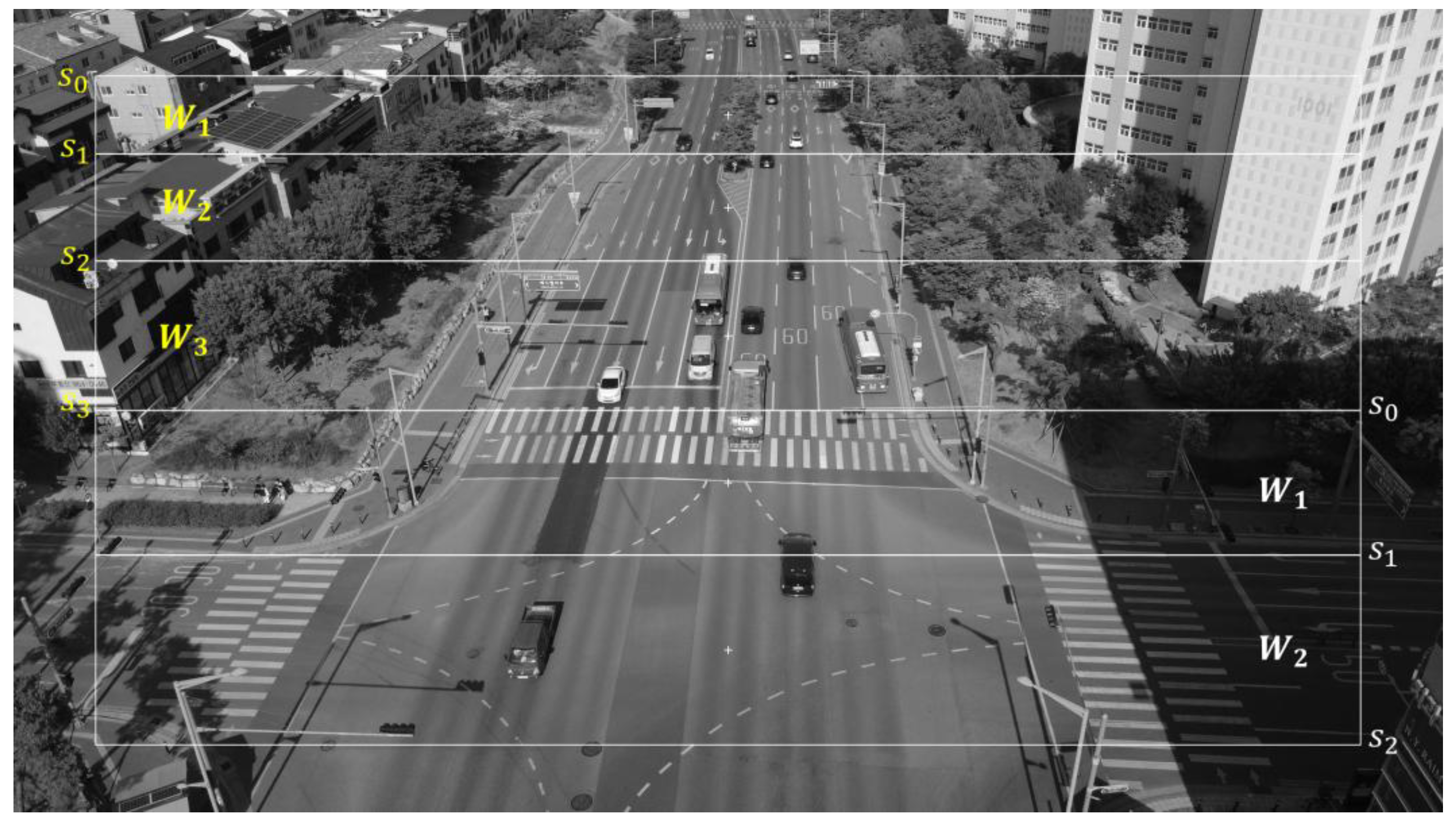
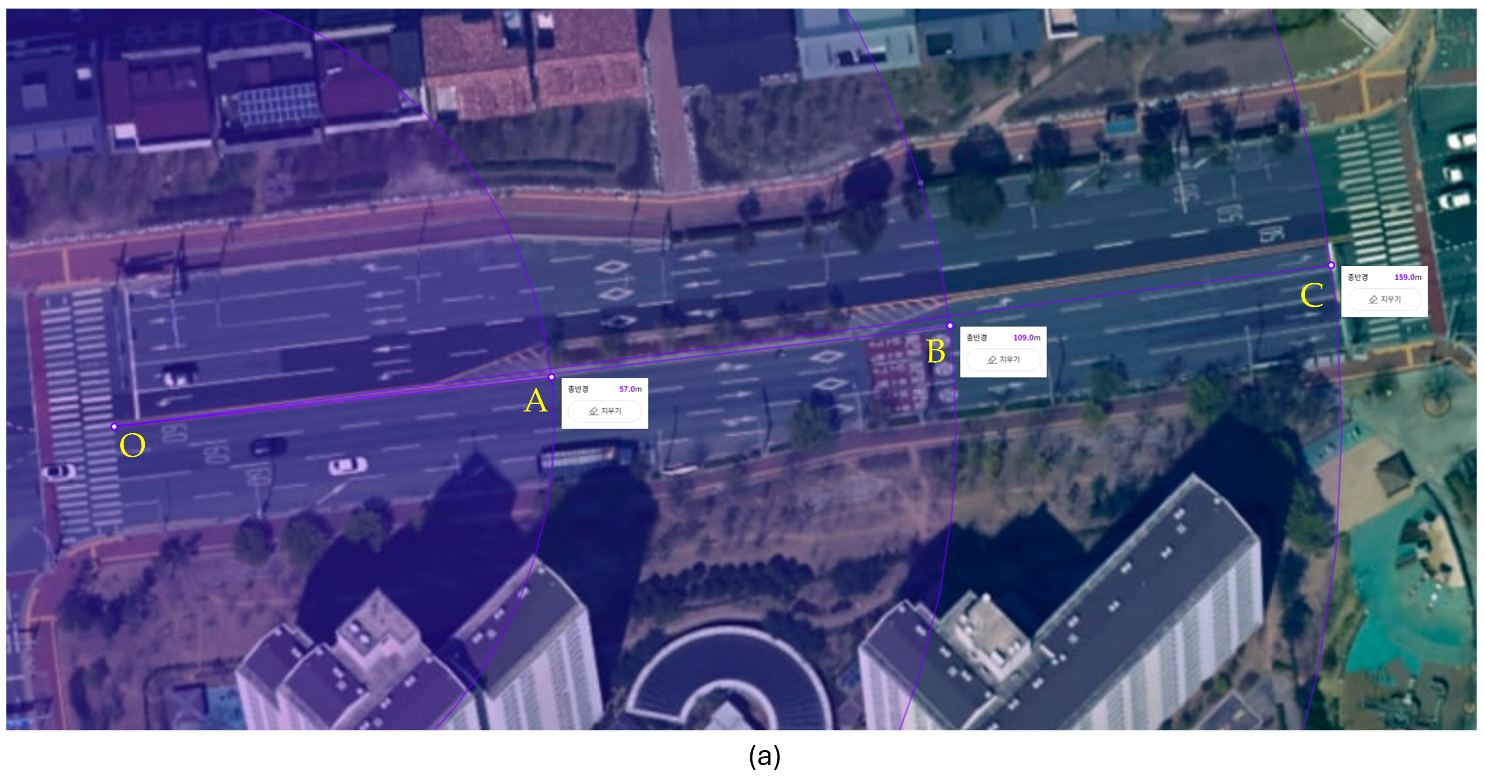
4.1. Scenario Description

A mini drone weighing less than 250 g (DJI Mini 4K) [34] flew along two different 150 m long roads and captured videos at 30 FPS with a frame size of 3840 × 2160 pixels. The drone altitude was maintained at 40 m during the flight, and the camera tilt angle was set to 60 degrees. The AFOV was assumed to be 64 degrees and 40 degrees in the horizontal and vertical directions, respectively.

Figure 7a is a commercially available satellite image of a vehicle road in an urban environment (Road 1) while Figure 7b is a vehicle road in a suburban environment (Road 2). Compared to the suburban road, the urban road has complex backgrounds and irregular terrain due to buildings and various artificial structures. Both figures also show three circles centered at Point O and passing through Points A, B, and C. The radius (distance) to each point is the ground truth for the drone’s flight distance. For Road 1 and Road 2, the distances from Point O to Point A are 57 m and 48 m, respectively, the distances between Point O and Point B are 109 m and 100 m, respectively, and the distances between Point O and Point C are 159 m and 150 m, respectively.

The drone starts from a stationary hovering Point O, reaches its maximum speed in normal flight mode before Point A, and then continues flying at a nearly constant speed passing near Points A, B, and C. The flights were repeated 10 times in different traffic conditions on each road.

Figure 8a and Figure 8b show sample video frames when the drone passes near Points O, A, B, and C on Roads 1 and 2, respectively. The optical center of the camera is marked with a white ‘+’, which is assumed to be the drone’s position. The frame numbers when the drone reaches the same radius as Points A, B, and C were manually determined from the video.

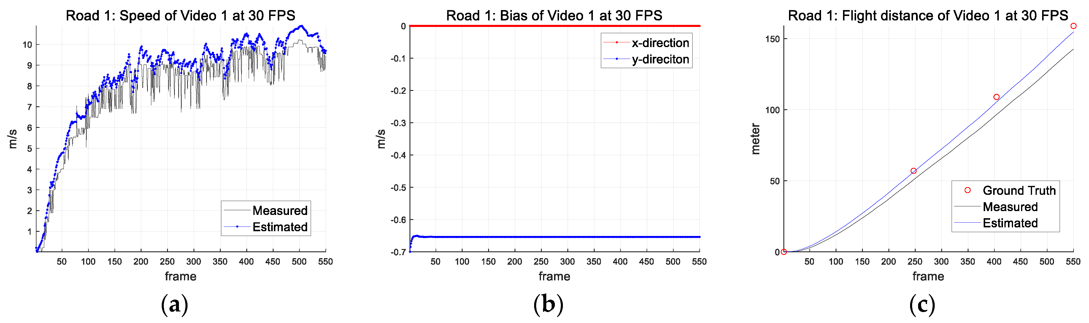
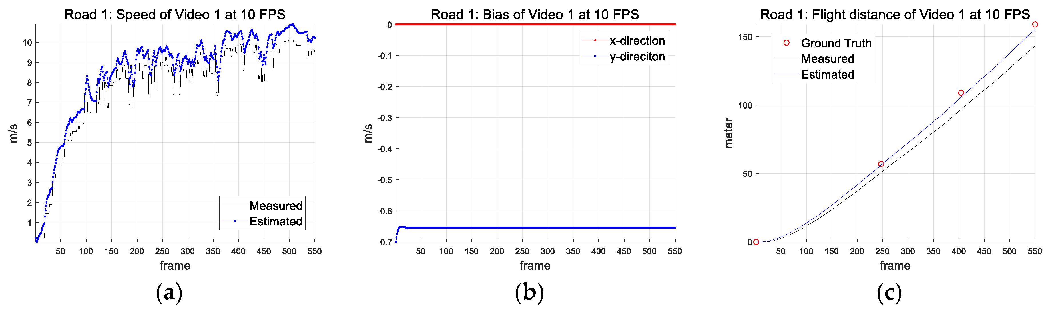
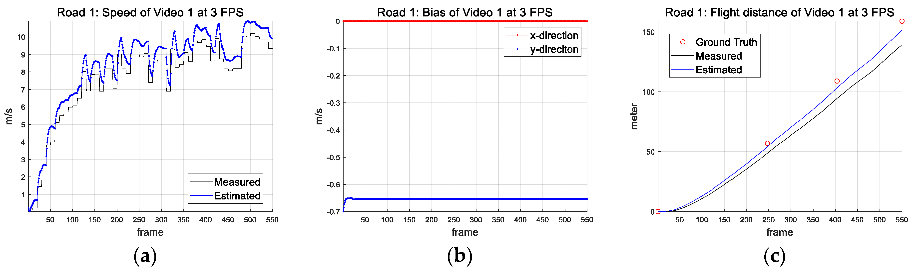
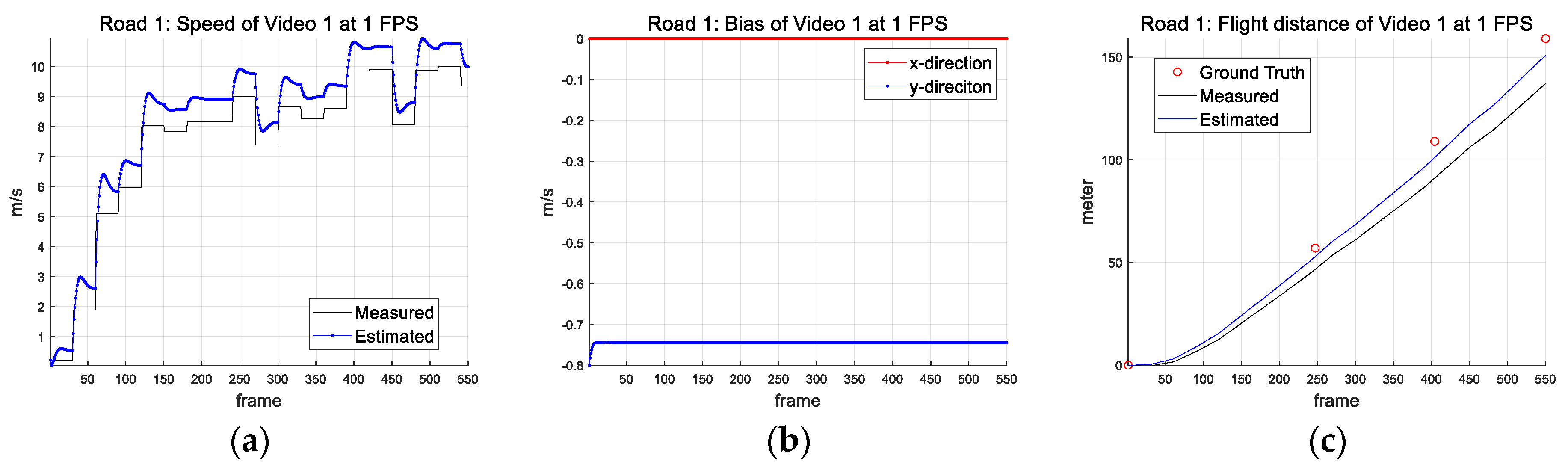
4.2. Drone State Estimation

Table 1. System parameters.

Parameter (Symbol) (Unit)	Road 1	Road 2
Sampling Time (T) (second)	1/30
Process Noise Std. (${\sigma }_{vx},{\sigma }_{vy}$) (m/s2)	(3, 3)
Bias Noise Std. (${\sigma }_{nx}, {\sigma }_{ny}$) (m/s)	(0.01, 0.1)
Measurement Noise Std. ($r_x,r_y$) (m/s)	(2, 2)
Initial Bias in x direction ($b_x\left(0\right)$) (m/s)	0
Initial Covariance for Bias ($P_x, P_y$) (m2/s2)	(0.1, 0.1)

shows the parameter values of the augmented-state Kalman filter. The sampling time is set to 1/30 s. The process noise standard deviation is set to 3 m/s² in both the x and y directions, the bias noise standard deviation is set to 0.01 and 0.1 m/s in the x and y directions, respectively, and the measurement noise standard deviation is set to 2 m/s in both the x and y directions. The initial covariance is set to the identical matrix except for the bias factors, which are set to 0.1 m²/s² in both the x and y directions. The initial bias in the x direction is set to 0 m/s for both roads while the initial bias in the y direction is set to −1.2 to 0.2 m/s depending on the frame-matching speed and the road traffic conditions. The 10 videos of Road 2 are divided into three groups (Group 1: Videos 1–3; Group 2: Videos 4 and 5; Group 3: Videos 6–10), and different initial values are applied as shown in

Table 2. Initial bias in y direction ($b_y\left(0\right)$) (m/s).

FrameMatching Speed (FPS)	Road 1	Road 2
		Group 1	Group 2	Group 3
30	−0.7	−0.3	0	0.2
10		−0.3	0	0.2
3		−0.3	0	0.2
1	−0.8	−0.7	−0.3	−0.1
0.5	−1	−1.2	−0.4	−0.4

. The same initial values are applied when the frame-matching speed is 30 FPS to 3 FPS, but the initial values decrease slightly as the speed decreases.

Table 3. Distance errors to Point C on Road 1.

FPS	Type	Video 1	Video 2	Video 3	Video 4	Video 5	Video 6	Video 7	Video 8	Video 9	Video 10	Avg.
30	Meas.	16.33	7.69	7.32	6.77	9.26	11.53	13.69	17.06	14.29	15.99	11.99
	Est.	4.25	4.55	4.95	5.54	3.10	0.89	1.46	4.50	2.02	3.95	3.52
10	Meas.	15.66	8.07	7.74	7.15	9.53	12.34	13.70	17.32	14.82	16.70	12.30
	Est.	3.59	4.15	4.51	5.15	2.82	0.08	1.47	4.79	2.57	4.63	3.38
3	Meas.	19.73	9.49	10.43	8.28	11.45	12.92	13.90	18.04	13.75	16.47	13.45
	Est.	7.65	2.71	1.81	4.00	0.91	0.51	1.69	5.50	1.53	4.34	3.07
1	Meas.	21.89	14.33	15.92	13.58	15.57	18.19	17.83	19.18	16.08	19.46	17.20
	Est.	8.16	0.40	1.96	0.39	1.47	4.03	3.92	4.85	2.12	5.68	3.30
0.5	Meas.	22.14	17.19	23.45	20.27	18.83	20.07	23.79	20.13	21.26	22.46	20.96
	Est.	5.03	0.16	6.06	2.87	1.25	2.41	6.45	2.23	3.89	5.31	3.57

and

Table 4. Distance errors to Point C on Road 2.

FPS	Type	Group 1			Group 2		Group 3					Avg.
		Video 1	Video 2	Video 3	Video 4	Video 5	Video 6	Video 7	Video 8	Video 9	Video 10
30	Meas.	11.96	4.60	5.47	0.35	0.46	3.94	4.84	5.10	4.21	11.96	5.29
	Est.	7.04	1.39	0.69	0.22	0.31	0.71	1.66	1.78	1.22	8.83	2.39
10	Meas.	12.00	5.37	5.55	0.87	0.74	3.56	4.39	4.65	4.22	11.16	5.25
	Est.	7.02	1.99	0.63	0.70	0.57	0.33	1.22	1.33	1.20	8.03	2.30
3	Meas.	14.32	6.09	5.89	2.23	1.91	2.30	2.48	3.09	2.63	8.56	4.95
	Est.	9.31	1.58	0.92	2.06	1.76	0.93	0.71	0.22	0.46	5.40	2.33
1	Meas.	17.78	8.45	11.18	5.73	4.31	1.15	1.26	1.46	1.41	5.18	5.79
	Est.	6.33	2.59	0.22	0.49	0.89	0.72	0.60	0.46	0.44	7.01	1.97
0.5	Meas.	23.11	12.74	18.76	8.08	6.88	5.43	8.49	6.21	6.84	0.59	9.71
	Est.	3.62	6.05	0.62	1.14	0.00	1.53	1.61	0.93	0.04	6.22	2.18

show the distance errors from Point O to C of 10 videos for Roads 1 and 2, respectively. The distance error is calculated as the absolute difference between the estimated flight distance and the actual distance (actual distance). In this case, the distance error is denoted as ‘Est’. Before Kalman filtering, the flight distance is calculated directly from the velocity obtained in Section 2, and the distance error is denoted as ‘Meas’. The average distance error to Point C before Kalman filtering is 11.99 m to 20.96 m for Road 1 and 4.95 m to 9.71 m for Road 2. The average distance error based on the estimated state for Road 1 is 3.07 m to 3.57 m, and the average distance error for Road 2 is 1.97 m to 2.39 m. As the frame-matching speed decreases, the average distance errors of the measured velocities increase, but the average distance errors of the estimated states remain at a similar level, showing the robustness of the proposed system.

Figure 9a shows the measured and estimated speeds of Video 1 of Road 1 when the frame-matching speed is 30 FPS. Figure 9b shows the biases in the x and y directions, and Figure 9c shows the actual, measured, and estimated distances to Points A, B, and C. Figure 10, Figure 11, Figure 12, and Figure 13 show the cases where the frame-matching speeds are 10, 3, 1, and 0.5 FPS, respectively. Figure 14, Figure 15, Figure 16, Figure 17 and Figure 18 show the same cases for Video 1 of Road 2.

Table 5. Average distance errors to Points A, B, C on Road 1.

FPS	Type	Point A (57 m)	Point B (109 m)	Point C (159 m)
30	Meas.	5.17	9.58	11.99
	Est.	1.68	2.35	3.52
10	Meas.	5.47	9.93	12.30
	Est.	1.68	2.34	3.38
3	Meas.	6.52	11.24	13.45
	Est.	1.51	2.39	3.07
1	Meas.	10.16	15.12	17.20
	Est.	3.74	4.81	3.30
0.5	Meas.	13.64	19.23	20.96
	Est.	5.66	6.40	3.57

and

Table 6. Average distance errors to Points A, B, and C on Road 2.

FPS	Type	Point A (48 m)	Point B (100 m)	Point C (150 m)
30	Meas.	3.25	4.27	5.29
	Est.	3.18	3.30	2.39
10	Meas.	2.88	4.07	5.25
	Est.	2.83	3.00	2.30
3	Meas.	1.99	3.29	4.95
	Est.	1.84	1.69	2.33
1	Meas.	2.41	4.23	5.79
	Est.	1.34	2.19	1.97
0.5	Meas.	6.41	6.87	9.71
	Est.	1.92	2.00	2.18

show the average distance errors to Points A, B, and C for Road 1 and Road 2, respectively. Table 5 shows a regular pattern, with the error increasing as the distance increases and the frame-matching speed decreases. However, Table 6 shows a somewhat irregular pattern in the average error in the estimated velocity as a function of distance or matching speed.

Twenty Supplementary Files are movies in MP4 format, and they are available online. Supplementary Videos S1–S10 show 10 videos capturing Road 1, and Supplementary Videos S11–S20 show another 10 videos capturing Road 2. The optical center of the camera is marked as ‘+’ in blue color. As the drone reaches the same radius as Points A, B, and C, the color of the mark is changed to white.

5. Discussion

The optimal windows aim to achieve uniform spacing in the real-world coordinates. The number of windows was set to three and two in the upper half and lower half, respectively, since the image-to-position conversion function is more nonlinear in the upper half than in the lower half. A larger number of windows can further reduce nonlinearities, but the displacements are computed with smaller templates and the local dependence increases. Similarly sized windows are also desirable because the velocity is computed by equally weighting displacements obtained from all templates, but further research on adaptive weighting is needed because the minimum detectable velocities vary depending on the window location as explained in Section 2.

The augmented-state Kalman filter with the NCA model improved the flight range accuracy from high to low meter-level error. The zero-order hold scheme provides similar accuracy regardless of the frame-matching speed.

It turns out that the initial bias setting is important. The suburban road can estimate the flight distance more accurately, but it is easily affected by the initial bias. Therefore, 10 videos of Road 2 were divided into three groups, and different initial biases in the y direction were applied to each group. The initial bias can be determined depending on the complexity and dynamics of the scene and the flatness of the terrain. If the frame-matching speed was slower, the initial bias should be lowered. They were chosen heuristically when better results were produced.

The computational complexity of the sum of normalized squared differences of $N_w$ templates is $\mathrm{O}\left({\displaystyle \frac{N^2}{N_w}}\right)$, where N is the number of pixels in the frame. This can be derived from the fact that the templates do not overlap each other and cover the entire image, and each template searches in a local region similar to the template size. When N is equal to 3840 × 2160 pixels, and $N_w$ is 5, $N^2/N_w$ is approximately 1.375 × 10¹³ operations per frame. If the processing is performed once every 2 s (0.5 FPS), the required computing power is 6.875 TFLOPS. This performance can be achieved through advanced embedded computing platforms that can be implemented on drones [35].

The proposed method requires only vision-based sensing, which has the advantages of GPS independence, low cost and low weight, passive sensing, and multi-functionality. The inherent scene dependency of vision-based methods is overcome by the augmented state estimation using the Kalman filter. As a result, the proposed method can achieve an average distance error of about 2 m after 150 m of flight when the terrain is flat and relatively simple. This technique can be used for multiple ground target tracking, where knowledge of the relative motion of the platforms is essential.

The proposed method appears to have strong potential for applications in a variety of fields, thus requiring further testing and analysis for more challenging missions, such as high-speed maneuvering flights or long-range flights at kilometer levels. Minimizing scene dependency prior to state estimation also remains a future challenge.

6. Conclusions

A novel frame-to-frame template-matching method is proposed. The optimal windows are derived from ray optics principles and the piecewise linear regression model. Multiple templates are obtained by their corresponding optimal windows. Therefore, the templates are scene or object independent, and no additional processes are required for template selection and update.

The Kalman filter adopts the NCA model, and its state is augmented to estimate the velocity bias of the drone. The zero-order hold method was applied for faster processing. The proposed technique achieves low average flight distance errors even at slow frame-matching speeds.

This technique can be useful when external infrastructure is not available such as in GPS-denied environments. It could be applied to a variety of fields, including automatic programmed flights or multiple ground target tracking using flying drones, which remains a subject of future research.

References

1. Zaheer, Z.; Usmani, A.; Khan, E.; Qadeer, M.A. Aerial Surveillance System Using UAV. In Proceedings of the 2016 Thirteenth International Conference on Wireless and Optical Communications Networks (WOCN), Hyderabad, India, 21–23 July 2016; pp. 1–7. [Google Scholar] [CrossRef]
2. Vohra, D.; Garg, P.; Ghosh, S. Usage of UAVs/Drones Based on Their Categorisation: A Review. J. Aerosp. Sci. Technol. 2023, 74, 90–101. [Google Scholar] [CrossRef]
3. Osmani, K.; Schulz, D. Comprehensive Investigation of Unmanned Aerial Vehicles (UAVs): An In-Depth Analysis of Avionics Systems. Sensors 2024, 24, 3064. [Google Scholar] [CrossRef] [PubMed]
4. Sekeroglu, B.; Tuncal, K. Image Processing in Unmanned Aerial Vehicles. In Unmanned Aerial Vehicles in Smart Cities; Al-Turjman, F., Ed.; Springer: Cham, Switzerland, 2020; pp. 167–179. [Google Scholar] [CrossRef]
5. Zhang, Z.; Zhu, L. A Review on Unmanned Aerial Vehicle Remote Sensing: Platforms, Sensors, Data Processing Methods, and Applications. Drones 2023, 7, 398. [Google Scholar] [CrossRef]
6. Mohammed, F.; Idries, A.; Mohamed, N.; Al-Jaroodi, J.; Jawhar, I. UAVs for Smart Cities: Opportunities and Challenges. Future Gener. Comput. Syst. 2019, 93, 880–893. [Google Scholar] [CrossRef]
7. Chen, C.; Tian, Y.; Lin, L.; Chen, S.; Li, H.; Wang, Y.; Su, K. Obtaining World Coordinate Information of UAV in GNSS Denied Environments. Sensors 2020, 20, 2241. [Google Scholar] [CrossRef] [PubMed]
8. Cahyadi, M.N.; Asfihani, T.; Mardiyanto, R.; Erfianti, R. Performance of GPS and IMU Sensor Fusion Using Unscented Kalman Filter for Precise i-Boat Navigation in Infinite Wide Waters. Geod. Geodyn. 2023, 14, 265–274. [Google Scholar] [CrossRef]
9. Qin, T.; Li, P.; Shen, S. VINS-Mono: A Robust and Versatile Monocular Visual-Inertial State Estimator. IEEE Trans. Robot. 2018, 34, 1004–1020. [Google Scholar] [CrossRef]
10. Campos, C.; Elvira, R.; Rodríguez, J.J.; Montiel, J.M.M.; Tardós, J.D. ORB-SLAM3: An Accurate Open-Source Library for Visual, Visual–Inertial, and Multi-Map SLAM. IEEE Trans. Robot. 2021, 37, 1494–1512. [Google Scholar] [CrossRef]
11. Kovanič, Ľ.; Topitzer, B.; Peťovský, P.; Blišťan, P.; Gergeľová, M.B.; Blišťanová, M. Review of Photogrammetric and Lidar Applications of UAV. Appl. Sci. 2023, 13, 6732. [Google Scholar] [CrossRef]
12. Petrlik, M.; Spurny, V.; Vonasek, V.; Faigl, J.; Preucil, L. LiDAR-Based Stabilization, Navigation and Localization for UAVs. In Proceedings of the 2021 International Conference on Unmanned Aircraft Systems (ICUAS), Athens, Greece, 15–18 June 2021; pp. 1220–1229. [Google Scholar]
13. Gaigalas, J.; Perkauskas, L.; Gricius, H.; Kanapickas, T.; Kriščiūnas, A. A Framework for Autonomous UAV Navigation Based on Monocular Depth Estimation. Drones 2025, 9, 236. [Google Scholar] [CrossRef]
14. Chang, Y.; Cheng, Y.; Manzoor, U.; Murray, J. A Review of UAV Autonomous Navigation in GPS-Denied Environments. Robot. Auton. Syst. 2023, 170, 104533. [Google Scholar] [CrossRef]
15. Zhang, J.; Singh, S. LOAM: Lidar Odometry and Mapping in Real-time. In Proceedings of the Robotics: Science and Systems (RSS), Berkeley, CA, USA, 9–13 July 2014. [Google Scholar]
16. Shan, T.; Englot, B.; Meyers, D.; Wang, W.; Ratti, C.; Rus, D. LIO-SAM: Tightly-Coupled Lidar Inertial Odometry via Smoothing and Mapping. In Proceedings of the 2020 IEEE/RSJ International Conference on Intelligent Robots and Systems (IROS), Las Vegas, NV, USA, 24 October 2020–24 January 2021; pp. 5135–5142. [Google Scholar]
17. Yang, B.; Yang, E. A Survey on Radio Frequency Based Precise Localisation Technology for UAV in GPS-Denied Environment. J. Intell. Robot. Syst. 2021, 101, 35. [Google Scholar] [CrossRef]
18. Jarraya, I.; Al-Batati, A.; Kadri, M.B.; Abdelkader, M.; Ammar, A.; Boulila, W.; Koubaa, A. GNSS-Denied Unmanned Aerial Vehicle Navigation: Analyzing Computational Complexity, Sensor Fusion, and Localization Methodologies. Satell. Navig. 2025, 6, 9. [Google Scholar] [CrossRef]
19. Gonzalez, R.C.; Woods, R.E. Digital Image Processing, 4th ed.; Pearson: Boston, MA, USA, 2018. [Google Scholar]
20. Brunelli, R. Template Matching Techniques in Computer Vision: A Survey. Pattern Recognit. 2005, 38, 2011–2040. [Google Scholar] [CrossRef]
21. Scaramuzza, D.; Fraundorfer, F. Visual Odometry [Tutorial]. IEEE Robot. Autom. Mag. 2011, 18, 80–92. [Google Scholar] [CrossRef]
22. Stauffer, C.; Grimson, W.E.L. Adaptive Background Mixture Models for Real-Time Tracking. In Proceedings of the IEEE Computer Society Conference on Computer Vision and Pattern Recognition (CVPR), Fort Collins, CO, USA, 23–25 June 1999; Volume 2, pp. 246–252. [Google Scholar]
23. Forster, C.; Pizzoli, M.; Scaramuzza, D. SVO: Fast Semi-Direct Monocular Visual Odometry. In Proceedings of the IEEE International Conference on Robotics and Automation (ICRA), Hong Kong, China, 31 May–7 June 2014; pp. 15–22. [Google Scholar] [CrossRef]
24. Kalal, Z.; Mikolajczyk, K.; Matas, J. Tracking-Learning-Detection. IEEE Trans. Pattern Anal. Mach. Intell. 2012, 34, 1409–1422. [Google Scholar] [CrossRef]
25. Hecht, E. Optics, 5th ed.; Pearson: Boston, MA, USA, 2017. [Google Scholar]
26. Yeom, S. Long Distance Ground Target Tracking with Aerial Image-to-Position Conversion and Improved Track Association. Drones 2022, 6, 55. [Google Scholar] [CrossRef]
27. Yeom, S.; Nam, D.-H. Moving Vehicle Tracking with a Moving Drone Based on Track Association. Appl. Sci. 2021, 11, 4046. [Google Scholar] [CrossRef]
28. Muggeo, V.M.R. Estimating Regression Models with Unknown Break-Points. Stat. Med. 2003, 22, 3055–3071. [Google Scholar] [CrossRef]
29. Bishop, C.M. Pattern Recognition and Machine Learning; Springer: New York, NY, USA, 2006. [Google Scholar]
30. OpenCV Developers. Template Matching. 2024. Available online: https://docs.opencv.org/4.x/d4/dc6/tutorial_py_template_matching.html (accessed on 5 June 2025).
31. Bar-Shalom, Y.; Li, X.R. Multitarget-Multisensor Tracking: Principles and Techniques; YBS Publishing: Storrs, CT, USA, 1995. [Google Scholar]
32. Simon, D. Optimal State Estimation: Kalman, H∞, and Nonlinear Approaches; Wiley-Interscience: Hoboken, NJ, USA, 2006. [Google Scholar]
33. Anderson, B.D.O.; Moore, J.B. Optimal Filtering; Prentice-Hall: Englewood Cliffs, NJ, USA, 1979. [Google Scholar]
34. Available online: https://dl.djicdn.com/downloads/DJI_Mini_4K/DJI_Mini_4K_User_Manual_v1.0_EN.pdf (accessed on 23 June 2020).
35. Zhao, J.; Lin, X. General-Purpose Aerial Intelligent Agents Empowered by Large Language Models. arXiv 2024, arXiv:2503.08302. Available online: https://arxiv.org/abs/2503.08302 (accessed on 7 June 2025).
Figure 1. Block diagram of drone state estimation.
Drones 09 00457 g001
Figure 2. Illustrations of coordinate conversion from image to real world: (a) horizontal direction, (b) vertical direction. The red box and line indicate the image plane.
Drones 09 00457 g002
Figure 3. Coordinate conversion functions: (a) horizontal direction, (b) vertical direction. The red circle indicates the center of the image.
Drones 09 00457 g003
Figure 4. (a) Three linear regression lines and two split points in the upper half, (b) two linear regression lines and one split point in the lower half.
Drones 09 00457 g004
Figure 5. Three optimal windows in the upper half of the sample frame and two optimal windows in the lower half. The centers of the windows are marked with a ‘+’.
Drones 09 00457 g005
Figure 6. Minimum detectable velocity: (a) horizontal direction, (b) vertical direction. The center position of the window is marked with a ‘+’.
Drones 09 00457 g006
Figure 7. Satellite image with ground truths of (a) Road 1, (b) Road 2.
Drones 09 00457 g007
Figure 8. Sample frames when the drone (the center of the camera) is at Point O or reaches the same radius as Points A, B, and C on (a) Road 1, (b) Road 2.
Drones 09 00457 g008
Figure 9. Road 1: Video 1 with 30 FPS frame-matching speed: (a) speed, (b) bias, (c) flight distance.
Drones 09 00457 g009
Figure 10. Road 1: Video 1 with 10 FPS frame-matching speed: (a) speed, (b) bias, (c) flight distance.
Drones 09 00457 g010
Figure 11. Road 1: Video 1 with 3 FPS frame-matching speed: (a) speed, (b) bias, (c) flight distance.
Drones 09 00457 g011
Figure 12. Road 1: Video 1 with 1 FPS frame-matching speed: (a) speed, (b) bias, (c) flight distance.
Drones 09 00457 g012
Figure 13. Road 1: Video 1 with 0.5 FPS frame-matching speed: (a) speed, (b) bias, (c) flight distance.
Drones 09 00457 g013
Figure 14. Road 2: Video 1 with 30 FPS frame-matching speed: (a) speed, (b) bias, (c) flight distance.
Drones 09 00457 g014
Figure 15. Road 2: Video 1 with 10 FPS frame-matching speed: (a) speed, (b) bias, (c) flight distance.
Drones 09 00457 g015
Figure 16. Road 2: Video 1 with 3 FPS frame-matching speed: (a) speed, (b) bias, (c) flight distance.
Drones 09 00457 g016
Figure 17. Road 2: Video 1 with 1 FPS frame-matching speed: (a) speed, (b) bias, (c) flight distance.
Drones 09 00457 g017
Figure 18. Road 2: Video 1 with 0.5 FPS frame-matching speed: (a) speed, (b) bias, (c) flight distance.
Drones 09 00457 g018