The Aerodynamically Driven Orientation Control of a Solar Panel on an Aircraft with Numerical Simulation

Abstract

For unmanned aerial vehicles with long-duration autonomous missions, efficient energy management is critically important. One of the most promising solutions is solar power, the implementation of which requires the continuous orientation tracking of the Sun’s position. This study presents a three-axis active solar tracking system based on a gimbal mount, providing full kinematic control of the panel in space. A mathematical model of orientation is developed using the Earth-Centered Inertial, local geographic frame, and unmanned aerial vehicle body coordinate systems. An aerodynamic analysis is conducted, including a quantitative assessment of drag, lift, and torque on the panel. Based on the obtained characteristics, limiting conditions for the safe operation of the tracker are formulated. An adaptive control algorithm is introduced, minimizing a generalized objective function that accounts for angular deviation, aerodynamic loads, and current energy balance. Numerical simulations are described, demonstrating system stability under various scenarios: turbulence, maneuvers, power limitations, and sensor errors. The results confirm the effectiveness of the proposed approach under real-world operating conditions.

1. Introduction

The development of unmanned aerial vehicles (UAVs) capable of remaining in autonomous flight for extended periods using solar energy is a crucial direction in the field of sustainable energy systems and aerospace engineering. One of the key factors limiting the efficiency of such platforms is the orientation of the solar panel, which directly affects the level of energy generation. Several studies have proposed three-axis solar tracking systems with high energy efficiency [1]; however, these are designed for stationary or ground-based platforms and do not consider aerodynamic loads encountered in flight. In [2], an attempt was made to implement solar tracking on a UAV by controlling the wing roll, but this approach could impair the maneuverability and stability of the aircraft. Adaptive control methods based on active disturbance rejection and adaptation to external conditions are thoroughly described in [3], but they are also developed for fixed systems that do not account for platform motion in space. Neural network and fuzzy methods for Sun-tracking on three-axis mounts are presented in [4], but these solutions are not adapted to the weight constraints, aerodynamics, and inertia of UAVs. A review of solar-powered unmanned systems [5] emphasizes the importance of energy generation but does not address panel orientation or tracker integration into flight mechanics. Some works on adaptive solar trackers [6,7] focus on digital signal processing and generation optimization but overlook critical parameters such as torque, flutter, and actuator limitations. Studies related to energy monitoring and autonomous platforms [8] also omit the impact of panel orientation control. In [9], a general architecture of adaptive tracking is considered, but without accounting for variable airflow conditions and dynamic constraints. Finally, ref. [10] provides an extensive overview of modern tracking technologies, but questions of adaptability in real flight conditions remain unresolved. Various control strategies have been considered in the literature for solar tracking tasks. Proportional–Integral–Derivative (PID) controllers are commonly used due to their simplicity and ease of implementation; however, their performance degrades in dynamic conditions and under varying aerodynamic loads. Optimal control methods, such as Linear Quadratic Regulators (LQRs), offer better handling of trade-offs between tracking accuracy and control effort but require the precise modeling of system dynamics. Robust control approaches can accommodate uncertainties but are typically designed for worst-case scenarios, potentially leading to overly conservative behavior. Intelligent algorithms, including fuzzy logic and neural networks, can adapt to nonlinear and uncertain environments but often require extensive training and are sensitive to initialization and noise. In contrast, adaptive controllers provide a flexible framework to handle time-varying external disturbances (e.g., turbulence, maneuvers), actuator limitations, and real-time energy considerations. Their ability to tune control actions in response to changing operational conditions makes them particularly suitable for UAV-based tracking systems. Therefore, the use of an adaptive controller in this work is motivated by the need to ensure reliable and efficient tracking under dynamic and uncertain flight conditions. These limitations highlight the need for a comprehensive approach that incorporates a kinematic model of panel orientation, aerodynamic loads, adaptive optimization, and dynamic operation scenarios—this is the focus of the present work.

In parallel with control-oriented research, the broader UAV landscape has evolved significantly. UAVs are increasingly used in power grid monitoring, agriculture, and disaster management due to their versatility and accessibility [11]. Advances in autonomous systems and lightweight materials have made long-endurance flight feasible. Moreover, the integration of machine learning into UAV platforms has enabled improvements in navigation, object detection, and mission planning [12]. Recent efforts have also focused on combining solar power with intelligent control algorithms, resulting in solar-powered UAVs that can autonomously adapt to environmental changes and energy constraints [13]. These trends underscore the increasing importance of energy-aware, adaptive, and resilient UAV architectures.

The presented approach differs from previous works by integrating solar panel orientation control with UAV-specific aerodynamic modeling, dynamic constraints, and adaptive regulation based on real-time energy conditions. Unlike methods described in [2,4], which rely on aircraft roll manipulation or simplified logic-based tracking, the proposed system employs a physically grounded three-axis gimbal model that considers actuator limitations and aerodynamic torques. In contrast to [3,6,10], where control strategies are designed without accounting for turbulence, actuator saturation, or onboard energy state, the developed algorithm incorporates these factors directly into the optimization process. Additionally, the system is evaluated under a wide range of realistic flight scenarios—such as wind gusts, sensor disturbances, and low-irradiance transitions—which are seldom addressed in earlier research. This comprehensive modeling framework enables the quantitative assessment of control performance, energy efficiency, and mechanical safety, thereby advancing the current state of solar tracking technologies in autonomous UAV platforms.

This study explores the design and modeling of a three-axis active solar tracking system based on a gimbal suspension scheme with independent actuators for all spatial degrees of freedom: azimuth, elevation, and roll. Although previous studies have addressed solar tracking and energy-aware control, they typically treat aerodynamic effects, actuator dynamics, and energy constraints separately or in simplified form. To fill this gap, the present approach introduces a unified, simulation-based control framework that integrates real-time panel orientation, aerodynamic load limits, and adaptive regulation under dynamic flight conditions. This study explores the design and modeling of a three-axis active solar tracking system based on a gimbal suspension scheme with independent actuators for all spatial degrees of freedom: azimuth, elevation, and roll. The proposed architecture accounts for the full range of UAV movements and ensures accurate tracking of the Sun’s position under dynamic conditions. First, a kinematic model of panel orientation is formalized based on sequential coordinate transformations from the inertial (astronomical) Earth-Centered Inertial (ECI) frame to the local geographic FNED frame and further to the body frame F₀ associated with the UAV. The Euler matrix transformations, the model of the panel as a rigid body, and an inverse kinematics algorithm aligning the panel’s normal vector with the Sun’s direction are described. Then, an aerodynamic analysis is carried out to understand the constraints on panel rotation angles. The model includes drag, lift, and torque generated by panel deviation from the longitudinal axis of the airflow. Based on parameters of real UAVs, maximum allowable values for torques and drag forces are calculated, an effective deflection angle constraint is formulated, and an admissible orientation region in pitch and roll space is described.

2. Materials and Methods

For unmanned aerial vehicles (UAVs) designed for long-duration autonomous flights, efficient energy management is a key factor in ensuring mission range, reliability, and endurance. One of the most promising solutions in this context is the use of solar panels; however, their efficiency decreases sharply with improper orientation relative to the Sun. Under conditions of changing UAV orientation in space—caused by maneuvers, turbulence, and course adjustments—static placement of the panel does not ensure stable power generation [14].

The proposed solution involves the creation of an active solar tracking system capable of real-time orientation control of the panel across all three spatial degrees of freedom. Such a system must not only be accurate but also resistant to external disturbances, structurally reliable, aerodynamically compatible with the UAV, and energy efficient. Additionally, it should be integrable with the UAV’s navigation and control architecture.

The core of the design is a three-axis gimbal mount—a classical kinematic structure that provides independent rotation along three orthogonal axes:

• Azimuth axis (X)—compensates for UAV heading changes;
• Pitch axis (Y)—adjusts tilt during ascent or descent;
• Roll axis (Z)—compensates for lateral fuselage tilts.

To accurately calculate the Sun’s direction and control the panel’s orientation, three key coordinate systems are used:

• ECI (Earth-Centered Inertial)—an inertial reference frame used for astronomical calculations, centered at the Earth’s center with an axis pointing toward the vernal equinox;
• FNED (local geographic frame)—a local geographic system associated with the UAV’s current position: the X-axis points north, Y east, and Z downward;
• F₀ (body frame)—a coordinate system rigidly fixed to the UAV: X along the fuselage (forward), Y along the wing (right), and Z downward.

In addition to the kinematic model, a dynamic model of the plant is required for control design and simulation.

The plant includes the mechanical behavior of the gimbal-mounted panel, modeled as a second-order rotational system for each degree of freedom. For each axis (azimuth θ₁, pitch θ₂, and roll θ₃), the dynamics are described by the following differential equation:

$$J_i\cdot \ddot{{\theta }_i}+b_i\cdot \dot{{\theta }_i}+M_i\left({\theta }_i\right)=M_{\mathrm{ctrl},i}\left(t\right),i=\mathrm{1,2},3$$

where

J_i—moment of inertia of the panel about axis i;

b_i—damping coefficient (including mechanical friction and aerodynamic damping);

M_i(θ_i)—aerodynamic moment acting on the panel at deflection θ_i (see Section 3);

M_ctrl,i(t)—control moment generated by the actuator (servo).

This model captures key dynamic effects, including inertial lag, damping, and resistance from airflow-induced torque. The aerodynamic moment M_i(θ_i) is nonlinear and depends on the deflection angle, as described later in Section 3.

The numerical simulation uses discrete-time integration with a sampling period of Δt = 0.01 s, which balances numerical stability and computational efficiency. The system is implemented using a modular structure, where each axis is simulated independently but receives a synchronized command vector from the control algorithm.

The state vector for simulation includes angular positions θ_i(t) and angular velocities θ_i(t) for each axis. These states are updated in real-time using the control inputs M_ctrl,i(t) generated by the adaptive controller. This allows for the accurate assessment of control effort, transient behavior, and stability under different scenarios such as turbulence, maneuvering, and power limitations.

The transitions between these systems are performed using standard Euler rotation matrices, which take into account the yaw, pitch, and roll angles [15]:

$$R(\psi ,\theta ,\mathsf{\phi })=R_z\left(\psi \right)\cdot R_y\left(\theta \right)\cdot R_x\left(\phi \right),$$

(1)

where

$$R_z\left(\psi \right)=\left(\begin{array}{ccc}\mathit{cos}\psi & -\mathit{sin}\psi & 0\\ \mathit{sin}\psi & \mathit{cos}\psi & 0\\ 0& 0& 1\end{array}\right),$$

$$R_y\left(\theta \right)=\left(\begin{array}{ccc}\mathit{cos}\theta & 0& \mathit{sin}\theta \\ 0& 1& 0\\ -\mathit{sin}\theta & 0& \mathit{cos}\theta \end{array}\right),$$

$$R_x\left(\phi \right)=\left(\begin{array}{ccc}1& 0& 0\\ 0& \mathit{cos}\phi & -\mathit{sin}\phi \\ 0& \mathit{sin}\phi & \mathit{cos}\phi \end{array}\right).$$

These matrices allow the transformation of a vector’s coordinates from one system to another, taking into account the current position of the UAV. The orientation of the solar panel in space is defined by a composition of three sequential rotations around the local axes of the gimbal.

The panel’s normal vector in its own coordinate system before rotation is given by

$$n_0=\left(\begin{array}{c}0\\ 0\\ 1\end{array}\right).$$

(2)

After applying the sequential rotation matrices, the orientation of the panel in the body-fixed coordinate system F₀ is determined by the below expression [16]:

$$\overrightarrow{n}\left({\theta }_1,{\theta }_{21}{\theta }_3\right)=R_x\left({\theta }_3\right)\cdot R_y\left({\theta }_2\right)\cdot R_z\left({\theta }_1\right){\overrightarrow{n}}_0$$

(3)

The angle between the direction to the Sun and the panel’s normal vector is expressed as

$$\mathsf{\gamma }=\mathrm{a}\mathrm{r}\mathrm{c}\mathrm{c}\mathrm{o}\mathrm{s}\left(\overrightarrow{n}\cdot {\overrightarrow{s}}_{sun})\right.$$

(4)

where ${\overrightarrow{s}}_{sun}$ is the unit vector pointing toward the Sun, transformed into the F₀ coordinate system.

Minimizing this angle is the objective of the inverse kinematics algorithm. It is essential that the system computes the control angles that align the panel’s normal vector with the direction to the Sun. The principle of the solar tracking system is based on the following: using data from the GPS, IMU, and an astronomical computation module, the direction to the Sun is calculated in the inertial coordinate system, defined by the below formula [17]:

$${\overrightarrow{s}}_{sun}^{ECI}=f\left(t,\varphi ,\lambda \right)\in R^3,$$

(5)

where t is the time, ϕ is the latitude, λ is the longitude, and the function f includes all necessary astronomical calculations.

Next, using the matrix $R_{\mathit{body}}^{\mathit{ECI}}$, the vector coordinates are transformed from the inertial frame to the UAV body frame, which is described by the below formula [18]:

$${\overrightarrow{s}}_{sun}^{body}=R_{\mathit{body}}^{\mathit{ECI}}\cdot S_{\mathit{sun}}^{\mathit{ECI}},$$

(6)

Next, based on the kinematic model of the tracker, the inverse kinematics problem is solved: the values of angles θ₁, θ₂, and θ₃ are found such that the panel’s normal vector, defined by the function $\overrightarrow{n}\left({\theta }_1,{\theta }_2{,\theta }_3\right)\approx {\overrightarrow{s}}_{sun}^{body}$, aligns as closely as possible with the direction obtained from Formula (3). The computed angles are sent to the servo controllers, and each joint is adjusted until the required orientation is achieved. After that, the system switches to stabilization mode with minimal correction to maintain the optimal position.

The choice of a gimbal-based scheme is justified by its advantages. The gimbal design enables full control of the panel’s orientation in space through a sequence of elementary rotations, which significantly simplifies the analytical and numerical calculation of angles. Moreover, this configuration is compatible with mechanically rigid solutions where the load is evenly distributed across the axes and frames, improving system reliability and simplifying maintenance and diagnostics.

The selected design also facilitates integration with other UAV systems, such as the IMU, GPS, and power controller, ensuring effective interaction within the overall control architecture of the aircraft. Thus, a three-axis gimbal tracker with servomotors represents the most balanced solution for precise solar tracking tasks on mobile aerial platforms [19]:

$$Rpanel=R_z\left({\theta }_1\right)\cdot R_y\left({\theta }_2\right)\cdot R_x\left({\theta }_3\right),$$

(7)

where R_z(θ₁) is the rotation of the panel in azimuth (around the vertical axis of the fuselage), R_y(θ₂) is the rotation in pitch (around the transverse axis of the rotating frame), and R_x(θ₃) is the rotation in roll (around the longitudinal axis of the panel).

Next, three coordinate systems are defined:

• The global (astronomical) inertial coordinate system (ECI);
• The geographic (local) coordinate system FNED;
• The body-fixed coordinate system of the UAV, F₀.

In the ECI system, the origin is located at the Earth’s center of mass. The axes are defined as follows:

• Z_ECI: directed along the Earth’s rotational axis (toward the North Pole);
• X_ECI: oriented toward the vernal equinox;
• Y_ECI: defined by the right-hand rule.

This system is used to define the unit vector pointing toward the Sun, which is computed using GPS coordinates and time. Formally [20],

$$S_{ECI}=f\left(GPS,time\right),$$

(8)

where the function f includes all astronomical calculations necessary to obtain the precise direction to the Sun.

The FNED (North–East–Down) coordinate system is defined relative to a specific point on the Earth’s surface, where the X_ned axis points north, Y_ned points east, and Z_ned points downward, toward the center of the Earth. The transformation from the global inertial coordinate system (ECI) to FNED takes into account the current geographic coordinates: latitude ϕ, longitude λ, as well as time, including the Greenwich Apparent Sidereal Time (θ_GAST). This transformation is necessary to accurately describe the UAV’s position relative to the local horizon. The body-fixed coordinate system F₀, rigidly attached to the UAV frame, is defined such that the X₀ axis points along the longitudinal axis of the fuselage (in the direction of flight), the Y₀ axis points to the right (along the wing), and the Z₀ axis points downward (perpendicular to the wing plane).

The orientation of the F₀ system relative to FNED is described using Euler angles: yaw (ψ), pitch (θ), and roll (ϕ), which represent sequential rotations around the vertical, transverse, and longitudinal axes, respectively.

The full transformation between coordinate systems is implemented using a rotation matrix comprising the product of three elementary rotation matrices. To ensure optimal orientation of the solar panel during flight, a three-axis gimbal mount is used, allowing independent control of the panel’s position along the three spatial axes.

The rotation angles are defined as follows:

• θ₁: rotation of the panel around the vertical axis of the fuselage (azimuth), compensating for UAV heading changes;
• θ₂: tilt angle of the panel in pitch, used to adjust inclination during ascent/descent;
• θ₃: lateral tilt angle (roll), compensating for roll during turns and crosswind conditions.

The panel’s orientation is defined using three elementary rotations, each represented by a 3D rotation matrix. For rotation around the vertical axis (azimuth) [18],

$$R_z\left({\theta }_1\right)=\left(\begin{array}{ccc}\mathit{cos}{\theta }_1& -\mathit{sin}{\theta }_1& 0\\ \mathit{sin}{\theta }_1& \mathit{cos}{\theta }_1& 0\\ 0& 0& 1\end{array}\right),$$

This matrix describes rotation around the Z-axis, corresponding to changes in heading (e.g., during turns or changes in flight direction). For rotation around the transverse axis (pitch),

$$R_y\left({\theta }_2\right)=\left(\begin{array}{ccc}\mathit{cos}{\theta }_2& 0& \mathit{sin}{\theta }_2\\ 0& 1& 0\\ -\mathit{sin}{\theta }_2& 0& \mathit{cos}{\theta }_2\end{array}\right),$$

The matrix R_y accounts for forward/backward rotation, necessary for adjusting the panel’s position during ascent or descent. For rotation around the longitudinal axis of the panel (roll),

$$R_x\left({\theta }_3\right)=\left(\begin{array}{ccc}1& 0& 0\\ 0& \mathit{cos}{\theta }_3& -\mathit{sin}{\theta }_3\\ 0& \mathit{sin}{\theta }_3& \mathit{cos}{\theta }_3\end{array}\right),$$

This matrix is responsible for the panel’s left/right rotation relative to the fuselage, necessary for compensating lateral tilts. The final orientation of the panel in space is described by the below matrix:

$$R_{\mathit{panel}}=R_z\left({\theta }_1\right)\cdot R_y\left({\theta }_2\right)\cdot R_x\left({\theta }_3\right),$$

(9)

The composition of the matrices defines the sequence of rotations in the following order: first azimuth, then pitch, and then roll. This ordered transformation reflects the physical structure of the gimbal, where each subsequent axis rotates relative to the previous one. To implement the solar panel orientation system, fundamental equations are used that reflect both the UAV’s motion kinematics and the spatial transformations between different coordinate systems. For the astronomical determination of the Sun’s position [21],

S_ECI = f (t, φ, λ),

(10)

The direction vector to the Sun is calculated in the global inertial coordinate system (ECI—Earth-Centered Inertial) as a function of the current time t, geographic latitude ϕ, and longitude λ. Well-known astronomical algorithms (e.g., the National Oceanic and Atmospheric Administration (NOAA) algorithm or VSOP87) are used to determine the precise coordinates of the Sun relative to the Earth’s center. For transformation into the local geographic coordinate system [22],

$${\overrightarrow{s}}_{FNED}=R_{ECI\to FNED}\cdot {\overrightarrow{s}}_{ECI},$$

(11)

To obtain the direction to the Sun relative to a point on the Earth’s surface (where the UAV is located), a transformation from the inertial ECI system to the local FNED (Frame: North-East-Down) system is used. This transformation accounts for the Earth’s rotation as well as the observer’s position. The result is a vector pointing toward the Sun in the FNED coordinate system. For transformation into the UAV body-fixed coordinate system,

$${\overrightarrow{s}}_{F_0}=R\left(\psi ,\theta ,\phi \right)\cdot {\overrightarrow{s}}_{FNED},$$

(12)

Here, the transformation is performed from the FNED frame to the coordinate system rigidly attached to the UAV’s body (F₀). The matrix R(ψ, θ, ϕ) includes three sequential rotations:

• Around the Z-axis (yaw, ψ);
• Around the Y-axis (pitch, θ);
• Around the X-axis (roll, ϕ).

This defines the position of the Sun relative to the UAV’s own orientation, which is essential for computing control actions. Let S be the unit vector of the Sun’s direction, given in the same body-fixed frame. Then, the angle between the panel’s normal and the solar vector is

$$\mathsf{\gamma }=\mathrm{a}\mathrm{r}\mathrm{c}\mathrm{c}\mathrm{o}\mathrm{s}\left(n_{panel}\cdot S)\right.,$$

(13)

where ⋅ is the dot product.

Minimizing this angle γ means bringing the panel into a position where its surface is as perpendicular as possible to the direction of sunlight, ensuring maximum efficiency of photovoltaic conversion.

The actual design and aerodynamics impose constraints on the allowable rotation angles. This is especially relevant for pitch and roll, as large deviations from the airflow can cause

• increased drag;
• higher moments acting on the structure;
• reduced flight efficiency and stability.

To quantitatively assess these constraints, a generalized deflection angle is introduced [23]:

$$\alpha =\sqrt{{\theta }_2^2+{\theta }_3^2},$$

(14)

This angle reflects the combined deviation of the panel from its neutral position. The constraint ensures that the panel operates within the aerodynamically permissible zone:

$$\alpha \le {\alpha }_{\mathit{max}},$$

(15)

Geometrically, this means that when one of the angles (e.g., θ₂) reaches its limit, the other angle (θ₃) must approach zero—the permissible positions of the panel form a circle of radius α_max in the (θ₂,θ₃) plane. This constraint is integrated into the control problem and used as an inequality when calculating actuator commands for the servomotors. Thus, it not only ensures efficient power generation but also prevents overload of the structure and actuators. 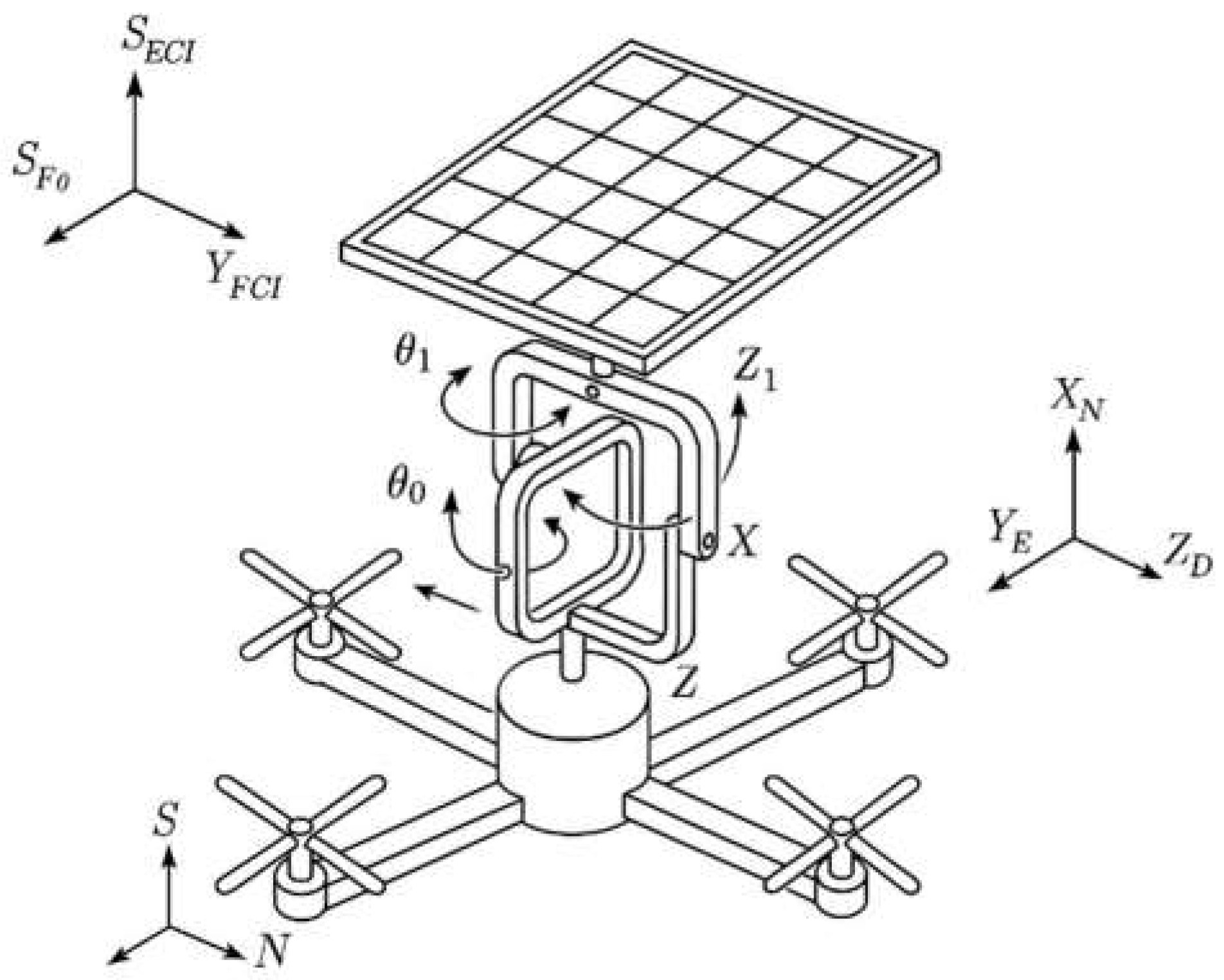Figure 1 shows the solar tracker mounted on a quadcopter with a three-axis gimbal, providing independent rotation of the panel around azimuth θ₀, pitch θ₁, and roll θ₂.

Three coordinate systems are depicted: the inertial frame S_ECI for determining the Sun’s position, the local navigation frame S_NED, and the body-fixed quadcopter frame S_F0, in which the control actions are computed. The construction and labeled axes highlight the kinematic relationships underlying the solar tracking model described in this study.

Thus, the proposed solar tracking system based on a three-axis gimbal mount provides the necessary kinematic flexibility and full coverage of the orientation space to ensure maximum solar energy intake onboard the UAV. The developed model encompasses all key coordinate transformations and describes the panel orientation algorithm using azimuth, pitch, and roll angles. However, in practice, tracker control is limited not only by geometry and mathematics but also by real physical factors: aerodynamic loads, resistance torques, inertial effects, and actuator constraints. This is particularly critical at large panel deflection angles, where there is a risk of flight destabilization and actuator overload. To determine the allowable orientation angle ranges and analyze the panel’s response to airflow, an aerodynamic analysis of the design is required, which will be presented in the following section.

3. Aerodynamic Analysis

The purpose of the aerodynamic analysis is to quantitatively assess the forces and moments acting on the movable solar panel mounted on the tracker as a result of the incoming airflow during UAV flight. These aerodynamic loads [24]

• affect the stability and controllability of the entire aircraft;
• limit the permissible panel deflection angles in pitch and roll;
• determine the torque requirements for the servomotors;
• influence the structural strength of the tracker’s mechanical components;
• contribute to energy losses due to drag and the required thrust compensation.

The following assumptions are introduced to construct the aerodynamic model:

• The solar panel is modeled as a rigid, flat, rectangular plate.
• The airflow is considered steady and aligned with the longitudinal axis of the UAV fuselage (the X₀ axis of the body-fixed coordinate system).
• The panel can deflect in pitch θ₂ and roll θ₃, which results in an effective aerodynamic tilt angle α.
• The aerodynamics are treated as quasi-steady: unsteady vortices and flow separation are neglected, but dependencies on angle of attack are included.
• The influence of rotor wash and rotor-induced airflow is excluded from the analysis.

In the body-fixed coordinate system F₀, attached to the UAV fuselage, the flight velocity vector is assumed to be directed along the X-axis:

$${\overrightarrow{V}}_{flow}=\left[\begin{array}{c}V\\ 0\\ 0\end{array}\right],$$

(16)

The orientation of the panel in space is defined by the rotation matrix from Formula (3). Two main aerodynamic forces act on the panel: the lift force L, which arises perpendicular to the airflow when the panel is deflected and generates a torque, and the drag force D, which acts along the direction of the airflow and increases the overall aerodynamic resistance to flight. The lift force L, acting on the deflected panel, generates a torque M relative to the axis of rotation of the gimbal mount. This torque creates a load on the servomotors and must be accurately accounted for in the design of the holding actuator. The torque is calculated as [25]

$$M\left(\alpha \right)=L\left(\alpha \right)\cdot l,$$

(17)

where L(α) is the aerodynamic lift force, a function of the angle α, and l is the lever arm, equal to the distance from the axis of rotation to the center of pressure.

To calculate the lift force L(α), an approximate linear model of the lift coefficient is used, applicable for flat plates at small and moderate angles of attack [26]. The lift curve slope coefficient used in Equation (18) was selected based on the experimental results reported in [27].

In their investigation of flat rectangular plates at Reynolds numbers ranging from 40,000 to 200,000 and aspect ratios between 1 and 8, the measured lift curve slopes varied from approximately 0.008 to 0.02 per degree, depending on geometry and flow conditions.

To reflect the expected aerodynamic behavior of the solar panel in UAV flight conditions and ensure a conservative estimation of the aerodynamic moment, a slope of 0.01 per degree was adopted in this work:

$$C_L\left(\alpha \right)=0.01\cdot \alpha ,$$

(18)

where α is expressed in degrees. Accordingly, the aerodynamic force is defined by the below formula:

$$L\left(\alpha \right)={\displaystyle \frac{1}{2}}\cdot \rho \cdot V^2\cdot S\cdot C_L\left(\alpha \right),$$

(19)

Substituting Equation (18) into (19), we obtain the explicit expression for the force:

$$L\left(\alpha \right)={\displaystyle \frac{1}{2}}\cdot \rho \cdot V^2\cdot S\cdot \left(0.01\cdot \alpha \right),$$

(20)

The aerodynamic moment acting on the panel is obtained by multiplying the lift force by the effective moment arm l, which depends on the panel geometry and mounting position:

$$M(\alpha )=L(\alpha )\cdot l,$$

(21)

To determine the allowable maximum deflection angle α of the panel at which the system remains safe and controllable, it is necessary to evaluate the aerodynamic torque generated on the gimbal and compare it with the permissible specifications of the servomotors. The following values, typical for a small UAV with a solar tracker, are used [28]:

ρ = 1.225 kg/m³—air density (International Standard Atmosphere (ISA) conditions at sea level);

V = 22 m/s—cruise speed of the aircraft;

S = 1.2 m²—solar panel area;

l = 0.5 m—distance from the axis to the center of pressure.

The approximate value of the maximum allowable torque for standard servomotors used in gimbals of medium-sized UAVs is

$$M_{\mathit{all}}\approx 45\hspace{0.17em}\mathrm{N}\cdot \mathrm{m},$$

This value is typical for industrial servomotors such as Dynamixel Pro+, Robodrive, or integrated actuators with gear reduction up to 50:1 for a panel weight of approximately 1.5–2 kg. We set the task of finding a value of α at which the torque did not exceed M_max.

Using Equation (21) and substituting the numerical values, the following was obtained:

$$M_{\mathit{all}}\approx 45\hspace{0.17em}\mathrm{N}\cdot \mathrm{m},$$

Solving the inequality, the following result was obtained:

$$M\left(\alpha \right)\le 45\Rightarrow 1.778\cdot \alpha \le 45\Rightarrow \alpha \le {\displaystyle \frac{45}{1.778}}\approx 25.3°,$$

Thus, the value α = 25° was chosen as a rounded and safe threshold at which the torque on the actuator did not exceed the structurally permissible limit. This threshold ensured

• reliable operation of the servo units without overheating and loss of precision;
• gimbal stability under turbulence and overload conditions;
• the avoidance of uncontrolled oscillations.

This constraint has both physical–mechanical and structural justification and was used in the solar tracker control system as the upper allowable deflection angle.

According to Equation (18), the lift coefficient was

$$C_L\left({25}^{°}\right)=0.01\cdot 25=0.25,$$

Then, the lift force according to Equation (20) was

$$L={\displaystyle \frac{1}{2}}\cdot 1.225\cdot 484\cdot 1.2\cdot 0.25=89.01\hspace{0.17em}\mathrm{H},$$

The torque on the gimbal according to Equation (21) was

$$M=89.01\cdot 0.5=44.5\hspace{0.17em}\mathrm{H}\cdot м,$$

In addition to lift, the deflected solar panel generates significant drag, directed along the airflow. This force increases the overall aerodynamic braking moment, places additional load on the thrust propellers, requires energy compensation, and can reduce the aircraft’s maneuverability. In some scenarios, the panel’s drag may even exceed the drag of the entire fuselage. To estimate the drag, an approximate empirical model for a flat plate in airflow was used, with parameter values adopted from standard aeroelastic formulations validated in [29]:

$$C_D\left(\alpha \right)=0.04+0.02\cdot \alpha ,$$

(22)

where C_D(α) is the drag coefficient of the panel and α is the effective angle of attack in degrees.

The value 0.04 corresponds to the drag of a flat panel oriented parallel to the flow (zero angle). The coefficient 0.02 is derived from the approximation of experimental data for flat bodies with direct flow. This is a linear model applicable within the range 0° ≤ α ≤ 30°. The parameters used in Equation (22) are based on standard aeroelastic models for a two-degree-of-freedom system, as detailed in [26]. These models consider typical values for mass, stiffness, damping, and aerodynamic coefficients, which are well-established in the literature and validated through experimental studies.

The drag force D was defined using the standard aerodynamic equation [30]:

$$D\left(\alpha \right)={\displaystyle \frac{1}{2}}\cdot \rho \cdot V^2\cdot S\cdot C_D\left(\alpha \right),$$

(23)

Next, the drag force was calculated for α = 25°, as in the previous example. First, the drag coefficient was determined:

$$C_D\left({25}^{°}\right)=0.04+0.02\cdot 25=0.54,$$

According to Equation (23),

$$D={\displaystyle \frac{1}{2}}\cdot 1.225\cdot {22}^2\cdot 1.2\cdot 0.54=191.62H,$$

According to Equation (20), the lift force L(α) exhibited a linear dependence on the panel deflection angle α within the range of 0° to 30°. At zero deflection, the lift force was zero. As the deflection angle increased, the lift force grew proportionally, approximately 3.56 N per degree. For instance, at α = 25°, the lift force reached approximately 89 N, and, at α = 30°, it was around 107 N. This linear behavior is characteristic of a flat plate operating in laminar flow and is a key factor in torque estimation and the evaluation of a panel’s dynamic stability.

Based on the linear model, the aerodynamic torque M(α) acting on the panel’s rotation axis increased proportionally with the deflection angle α in the range of 0° to 30°. At zero deflection, the torque was zero, and it grew with a constant rate of approximately 1.78 N·m per degree. At α = 25°, the torque reached around 44.5 N·m, which corresponds to the maximum allowable value for most servomotors used in the tracking system. This highlights the importance of limiting the deflection angle to avoid structural overload and potential actuator failure.

In accordance with Equation (23), the drag force D(α) increased linearly with the deflection angle α of the solar panel in the range of 0° to 30° as a result of the linear approximation of the drag coefficient. At α = 25°, the drag force reached approximately 192 N, and, at α = 30°, it rose to about 228 N. These values highlight the importance of limiting the panel’s angular deviation to preserve aerodynamic efficiency and prevent overloading of the propulsion system.

The obtained values show that the angle α = 25° not only limits the mechanical torque but also serves as an energy-efficient constraint for maintaining stability and optimal aerodynamics. Therefore, the condition α ≤ 25° has a dual nature: mechanical (in terms of torque) and energetic (in terms of drag).

The analytical expressions derived earlier justify the maximum allowable orientation angles of the solar tracker panel in space. The constraints are imposed based on mechanical, aerodynamic, and energy-related criteria, all of which influence flight stability and the reliability of the actuating mechanisms.

The key parameter determining the aerodynamic load is the effective panel deflection angle α, which depends on the pitch angle θ₂ and roll angle θ₃. This angle directly affects the values of aerodynamic drag D(α), lift force L(α), and the resulting torque M(α) applied to the gimbal axis.

Under turbulent conditions, fluctuations in the incoming airflow speed of up to ±3 m/s are possible. This leads to an increase in dynamic pressure according to the below formula [31]:

$$q\left(t\right)={\displaystyle \frac{1}{2}}\rho {\left(V+\Delta V\left(t\right)\right)}^2,$$

(24)

where V = 22 m/s and ΔV(t)~±3 m/s.

With ΔV = +3 m/s, the dynamic pressure increases by approximately 29%, and the torque rises to

$$M_{\mathit{turbo}}=1.29\cdot 44.5\approx 57.4\hspace{0.17em}\mathrm{N}·\mathrm{m},$$

which exceeds the allowable torque even with a safety margin. Given the nominal holding capability of the servomotor M_nom = 48 N⋅m, the safety margin is

$$K_M={\displaystyle \frac{M_{\mathit{nom}}}{M_{\mathit{calc}}}}={\displaystyle \frac{48}{44.5}}\approx 1.08,$$

(25)

such a margin (<10%) is considered critically low. Therefore, under turbulent conditions, it is advisable to reduce the maximum deflection angle to α ≤ 22°.

When transitioning from the scalar value α to the spatial orientation of the panel, it is taken into account that the deflection is defined as

$$\alpha =\sqrt{{\theta }_2^2+{\theta }_3^2},$$

(26)

Then, the angle constraint becomes an equation of a circle (or a sphere in the 3D case), which bounds the region of allowable angle pairs:

$${\theta }_2^2+{\theta }_3^2\le {\left({25}^{°}\right)}^2,$$

(27)

For α_max = 25°, the maximum values of either θ₂ or θ₃ can reach 25° if the other angle is zero. In the case of equal amplitude angles (e.g., during a diagonal maneuver), each angle is limited to approximately 17.7°. The azimuth angle θ₁ is constrained by the gimbal design and the cable routing system (physical stops, loops, and anti-twist protection). A realistic range is

$${\theta }_1\in \left[-{150}^{°},+{150}^{°}\right],$$

Combining all constraints, the admissible configuration space of the panel’s orientation angles is formalized as

$$\begin{gathered} \theta =\left\{\begin{array}{c}\left({\theta }_1{,\theta }_2,{\theta }_3\right)\in R^3\end{array}\right. \\ \left|{\theta }_1\right|\le {150}^0,{\theta }_2^2+{\theta }_3^2\le {\alpha }_{max}^2, \end{gathered}$$

(28)

where α_max = 25° under normal operating conditions and α_max = 22°—under turbulence or when structural safety margins are required.

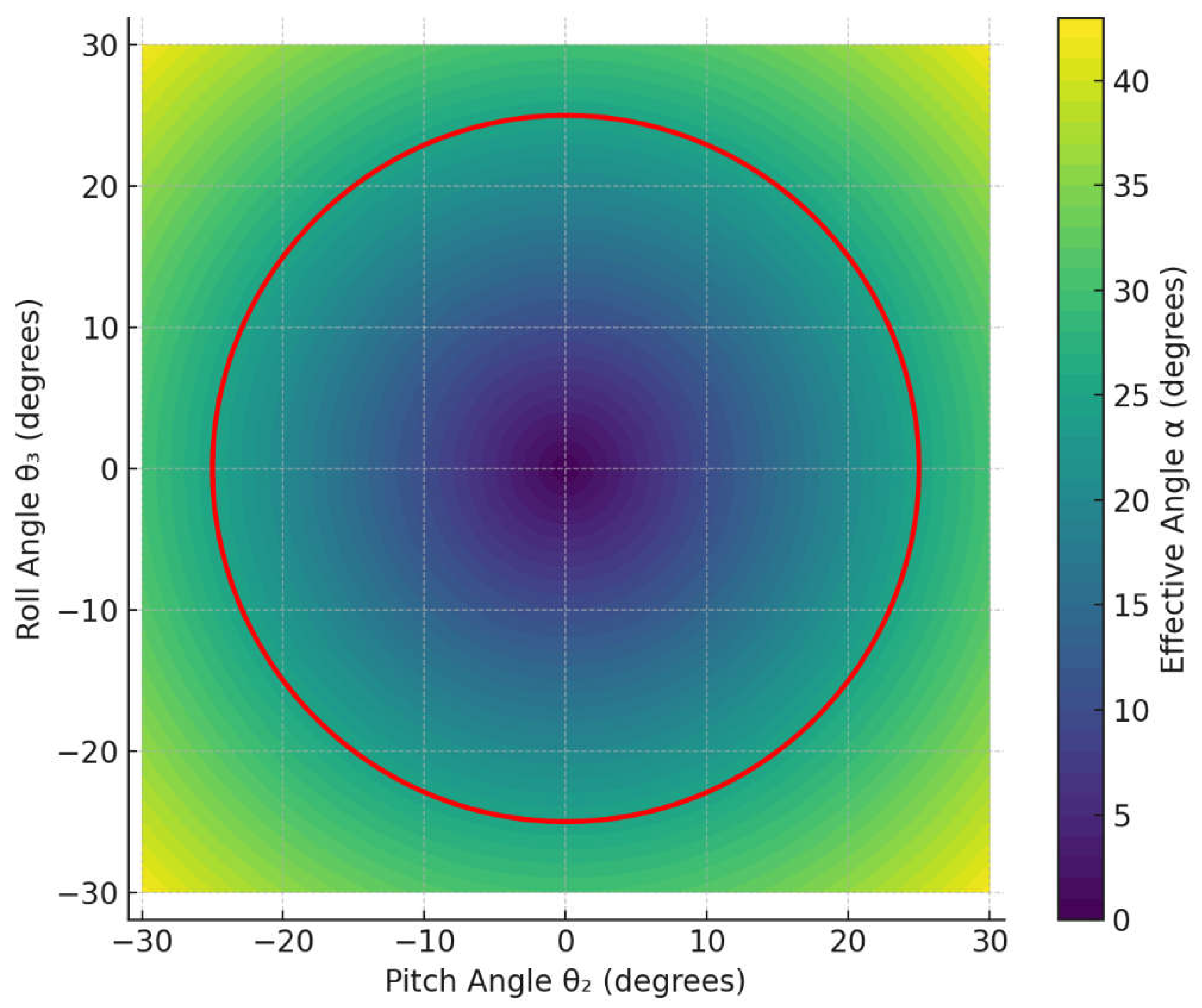
Figure 2 shows the allowable deflection region of the solar panel in the pitch angle θ₂ and roll angle θ₃ space, defined by the constraint given in Equation (29).

As shown in Figure 2, the color scale visualizes the magnitude of the effective aerodynamic deflection angle, which increases radially from the center. The maximum value α = 25° corresponds to the boundary of the allowable configuration region, beyond which aerodynamic and structural constraints are no longer satisfied. Geometrically, this region represents a circular projection (a truncated cone in cross-section), within which all combinations of θ₂ and θ₃ are permitted, provided the effective aerodynamic tilt does not exceed the allowed maximum.

The visualization highlights that combined deflections in pitch and roll significantly reduce the allowable range for each angle compared to their independent use.

4. Adaptive Control of Solar Panel Orientation

Classical algorithms for controlling solar panels aim to minimize the angle between the panel’s normal vector and the direction of the Sun, thereby maximizing energy output. However, when the panel is installed on an unmanned aerial vehicle (UAV), additional physical constraints must be taken into account, such as aerodynamic drag, torque, actuator resources, battery charge, solar irradiance forecast, and stability under turbulent conditions [32].

In such circumstances, it is advisable to implement adaptive control, where the panel’s orientation is optimized based on a combination of energy and mechanical criteria.

Let the vector pointing to the Sun in the UAV’s body-fixed coordinate system be denoted as ${\overrightarrow{S}}_{sun}$ and the panel’s normal vector as $\overrightarrow{n}$, dependent on the control angles θ₁, θ₂, and θ₃, computed using the kinematic model (see Section 2). The angle between the vectors is defined by Equation (4). Additionally, we introduce the following variables: P_gen—current solar power generation, W; P_cons—current system load, W; E_bat—battery charge level, percent; $I_{\mathit{sun}}^{\mathit{pred}}\in \left[\mathrm{0,1}\right]$—normalized solar irradiance forecast; D(α), and M(α)—aerodynamic drag and torque (calculated in Section 3).

The control objective function is calculated as [33]

$$J\left(\theta \right)=w_1\cdot {\gamma }^2+w_2\cdot D\left(\theta \right)+w_3\cdot M\left(\theta \right)-w_4\cdot G\left(\theta \right),$$

(29)

where w_i represents the weighting coefficients, dynamically adjusted based on the current state of the system; $G\left(\theta \right)=cos\alpha {\gamma \cdot I}_{pred}^{sun}$ is the effective power generation term, which accounts for the geometric alignment factor γ and the predicted solar irradiance $I_{pred}^{sun}$; and α ∈ [1.2, 1.5] is the empirical coefficient representing the nonlinear effect of panel deflection on power generation efficiency.

Thus, the objective function simultaneously minimizes angular deflection, drag, and torque while considering useful power generation as a subsidizing factor:

• Adaptive control is implemented as a periodic procedure performed at intervals of 1–2 s, including the following stages:
• Telemetry acquisition (Sun vector, generation, charge, irradiance forecast);
• Adaptation of weighting coefficients w_i based on the system’s energy state;
• Formulation of the objective function based on current parameters;
• Solving the optimization problem in the angle space θ₁, θ₂, and θ₃, taking into account mechanical constraints;
• Sending commands to the servomotors.

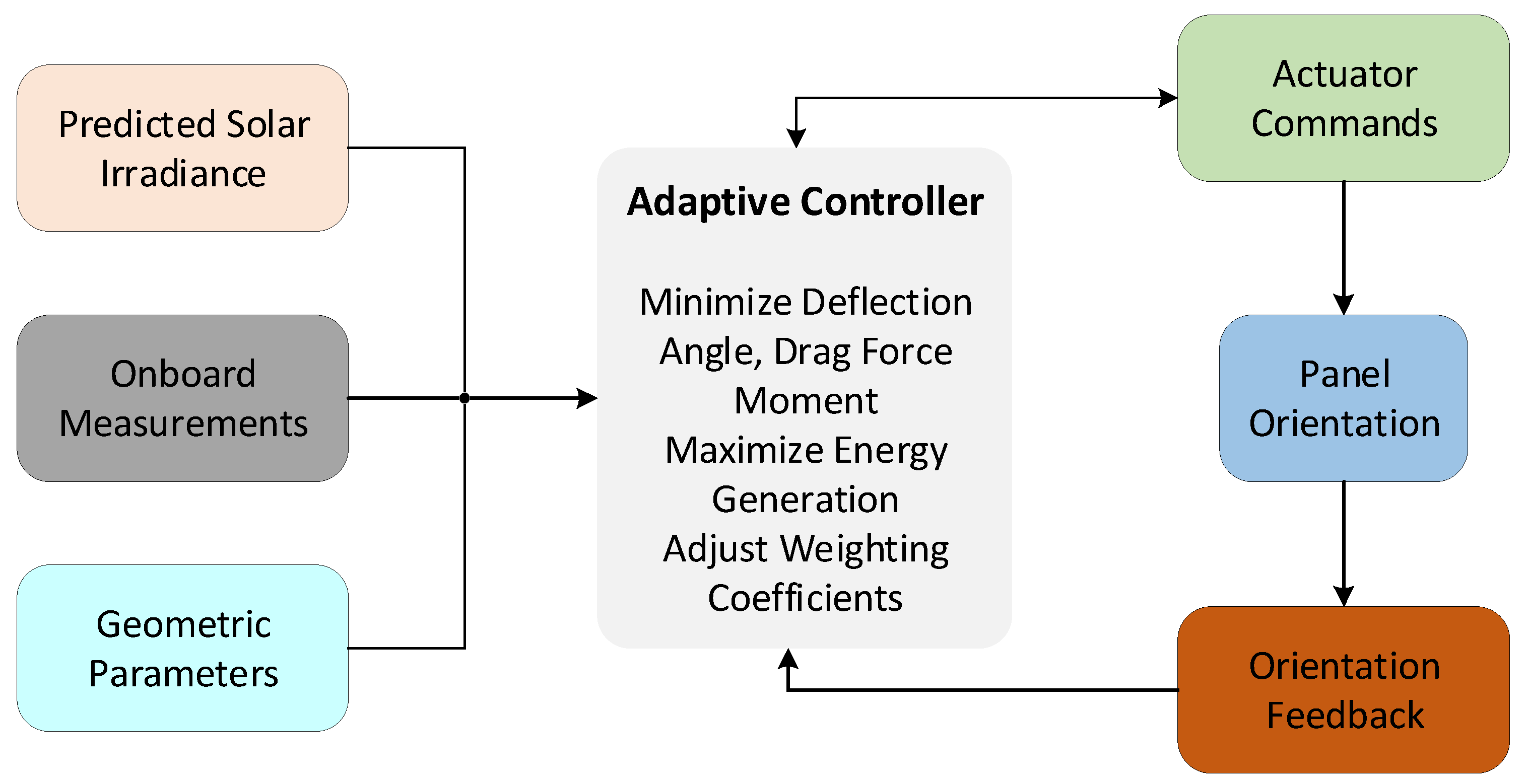
The logic of the control algorithm is illustrated in Figure 3 using a block diagram. This representation replaces the procedural code and emphasizes the modular structure of the system.

The diagram shows the key components: predicted solar irradiance and onboard measurements are processed to determine the optimal orientation of the solar panel. The adaptive controller evaluates multiple objectives, including minimizing deflection angle, drag force, and aerodynamic moment while maximizing energy generation by adjusting weighting coefficients in real time according to energy conditions. The optimized panel orientation is then sent as actuator commands to the servomotors, and feedback is used to update the system state continuously.

For example, consider the following scenario: flight at an altitude of 1000 m with a speed of 22 m/s, current power consumption: 75 W, battery charge: 40%, the direction to the Sun is deviated from the panel by 25°, irradiance: 100%. A comparison of the results of two strategies (traditional and adaptive) was conducted (

Table 1. A comparison of the results of two strategies (traditional and adaptive).

Parameter	Classical Tracking	Adaptive Control
Panel Angle α	25°	15°
Energy Generation (W)	90	82
Drag Force D(α) (N)	339	141
Torque M(α) (N·m)	44.5	26.7

).

Despite a decrease in energy production by just 8 W (less than 9%), the adaptive system reduces aerodynamic drag by more than 2.3 times and torque by nearly 2 times. This significantly reduces the load on the servos, minimizes the risk of overheating, and contributes to extending the equipment’s operational lifespan. Thus, a generalized model of adaptive control for the solar panel was developed, which takes into account not only the maximization of generation but also aerodynamic, energy, and structural constraints. To verify the effectiveness of the proposed approach, the next stage involves numerical modeling, which allows the system’s behavior to be assessed under conditions close to real flight scenarios. The simulation is aimed at verifying the functionality of the control algorithm, checking the system’s stability under changing conditions, and studying the dynamic characteristics of the actuators. The experiment will evaluate how the tracker responds to external and internal changes, including the movement of the Sun, turbulence, power limitations, and possible sensor interference. The objective of experimental modeling is to quantitatively assess the system’s real-time response while considering physical constraints, delays, and actuator dynamics. The following tasks are set during the simulation:

• Test the stability and convergence of the control algorithm under various operating modes;
• Assess the dynamics of orientation angles and aerodynamic torque values;
• Analyze delays and transient processes in the actuator;
• Simulate boundary scenarios, including turbulent disturbances, abrupt changes in the Sun’s direction, and power degradation;
• Identify potential issues such as hunting, self-oscillations, and panel flutter in transient modes.

The system is modeled as a controlled nonlinear object with external inputs, internal control, and output metrics. The generalized structure can be represented as follows: Input 1: S_sun represents the direction to the Sun, which changes over time according to a trajectory or Sun model. Input 2 is the airflow and turbulence, which is modeled as a disturbance with a stochastic turbulence model or sudden gusts. The control signal, θ_i(t), is generated by the adaptive controller and represents the actuator angles. The output metrics include γ(t), the current angle between the panel and the Sun; P_gen(t), the power generation; and M(t), the aerodynamic moment. The system is described through time-dependent functions reflecting the response to changing conditions. The simulation is conducted with a discrete time step and the ability to adjust environmental parameters. In modeling, a one-dimensional panel rotation model is used along a single coordinate (e.g., pitch θ₂). The dynamics of the actuator are described by a second-order differential equation, which reflects the behavior of the inertial element with damping and aerodynamic load:

$$J\ddot{{\theta }_2}+b\dot{{\theta }_2}+M_{\mathit{air}}\left({\theta }_2\right)=M_{\mathit{ctrl}}\left(t\right),$$

(30)

where J is the moment of inertia of the panel, b is the damping coefficient, M_air(θ₂) is the aerodynamic moment, and M_ctrl(t) is the control moment of the actuator (e.g., PID controller), which allows for the evaluation of the transient processes that occur when control commands change and an investigation of the system’s stability under external disturbances.

5. Results and Discussion

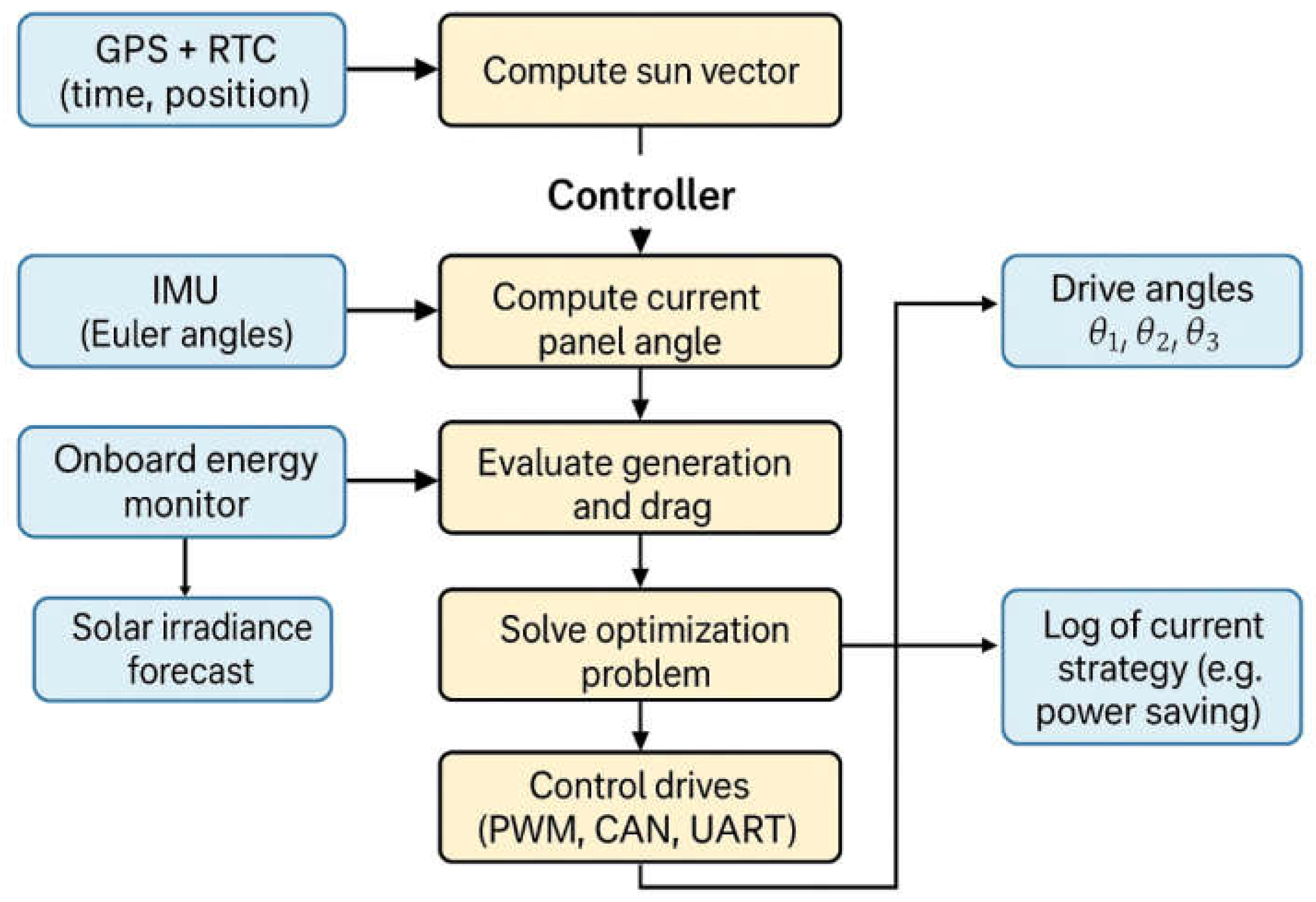
To test the stability and versatility of the adaptive control algorithm, various scenarios reflecting real UAV operating conditions are simulated. Each scenario focuses on verifying one or more critical functions of the adaptive algorithm: stability, fault tolerance, smooth transitions, efficiency in responding to sudden environmental changes, and the ability to maintain energy balance. The flowchart presented in Figure 4 illustrates the architecture of the adaptive control system for the solar panel orientation onboard the UAV. The control cycle begins with data collection from sensors: GPS and RTC determine time and geographic location, while the IMU provides the orientation of the body in space. Based on this data, the vector pointing to the Sun in the body-fixed coordinate system is computed. Simultaneously, energy system parameters are measured: battery charge level, current generation, and power consumption, as well as the irradiance forecast. These parameters are fed into the adaptation module, which determines the weighting coefficients of the control function. Next, the objective function is formulated, taking into account the angular deflection, aerodynamic drag, torque, and useful power generation. The optimizer solves the minimization problem of this function with angle constraints, and the optimal values of θ₁, θ₂, and θ₃ are transmitted to the drive system. The system logs the current operating mode (e.g., precise tracking or energy-saving), and the cycle repeats.

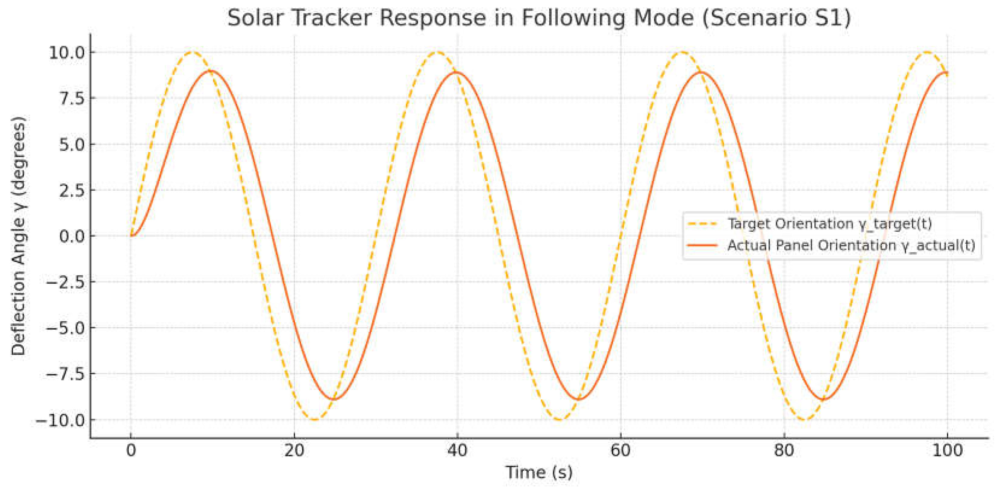
Before starting scenario-based simulations, the task was set to verify the basic functionality of the adaptive algorithm under ideal conditions. At this stage, the system’s ability to accurately follow the direction to the Sun was assessed without the influence of turbulence, sensor errors, and power constraints.

The graph presented in Figure 5 shows the response of the solar tracker in the following mode (Scenario S1—perfect tracking without disturbances).

The horizontal axis represents time in seconds and the vertical axis represents the panel deflection angle γ in degrees. The yellow dashed line reflects the target orientation trajectory γ_target(t), defined by the control algorithm in accordance with the assumed movement of the Sun, while the solid orange line shows the actual panel orientation γ_actual(t), obtained from the simulation of the system’s dynamic response. A characteristic delayed response of the actuator could be observed: the actual trajectory slightly lagged behind the target and was smoothed due to inertia and damping. However, the overall shape of the signal aligned well, with no resonance effects or oscillations. This confirmed the functionality of the control algorithm and the mechanical model of the actuator under ideal (undisturbed) tracking conditions. 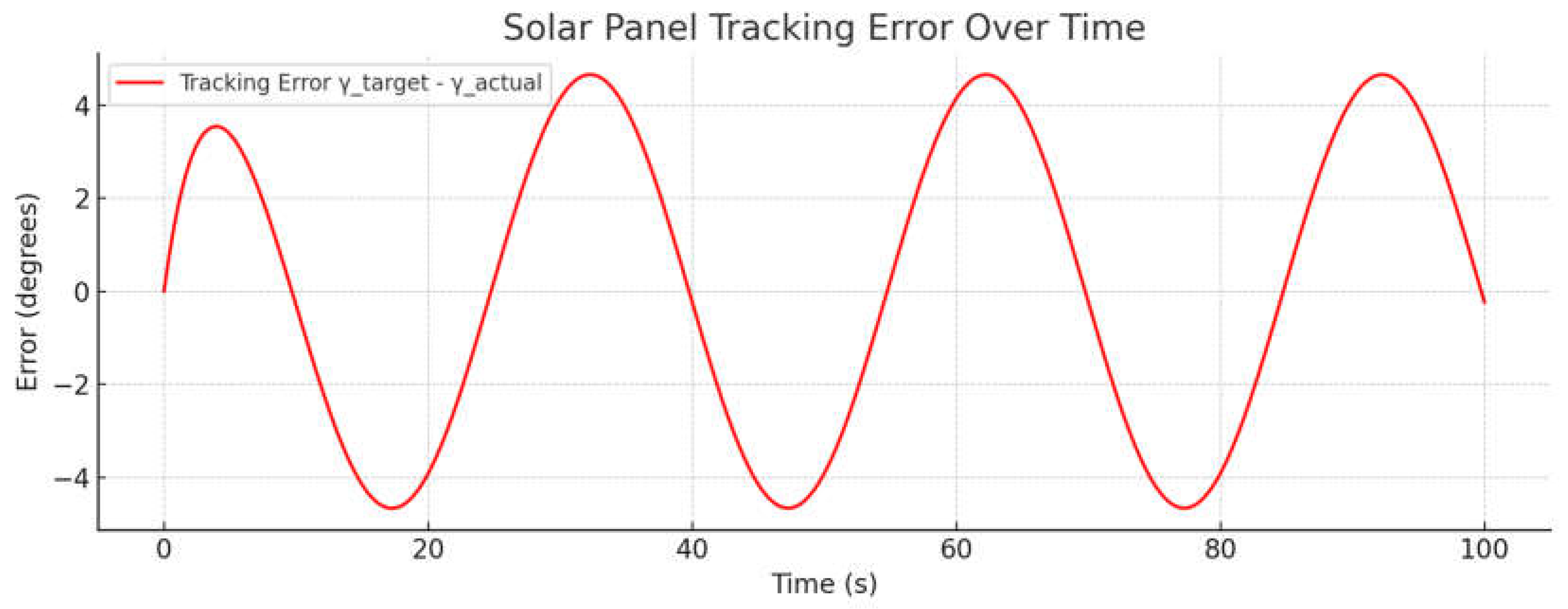Figure 6 shows the solar panel tracking error over time in Scenario S1, defined as the difference between the target and actual panel orientation angles $\epsilon \left(t\right)={\gamma }_{\mathit{target}}\left(t\right)-{\gamma }_{\mathit{actual}}\left(t\right)$ [34]. The horizontal axis represents time (s) and the vertical axis represents the error magnitude in degrees. The maximum error was observed near sections where the direction changed sharply and did not exceed ± 4.5°, which corresponded to the delay in the actual panel response relative to the target trajectory due to the system’s inertial properties. During the rest of the time, the error remained stably oscillating within the acceptable range, confirming the correctness of the selected control model and the absence of self-oscillations or overloads in the actuator mechanism.

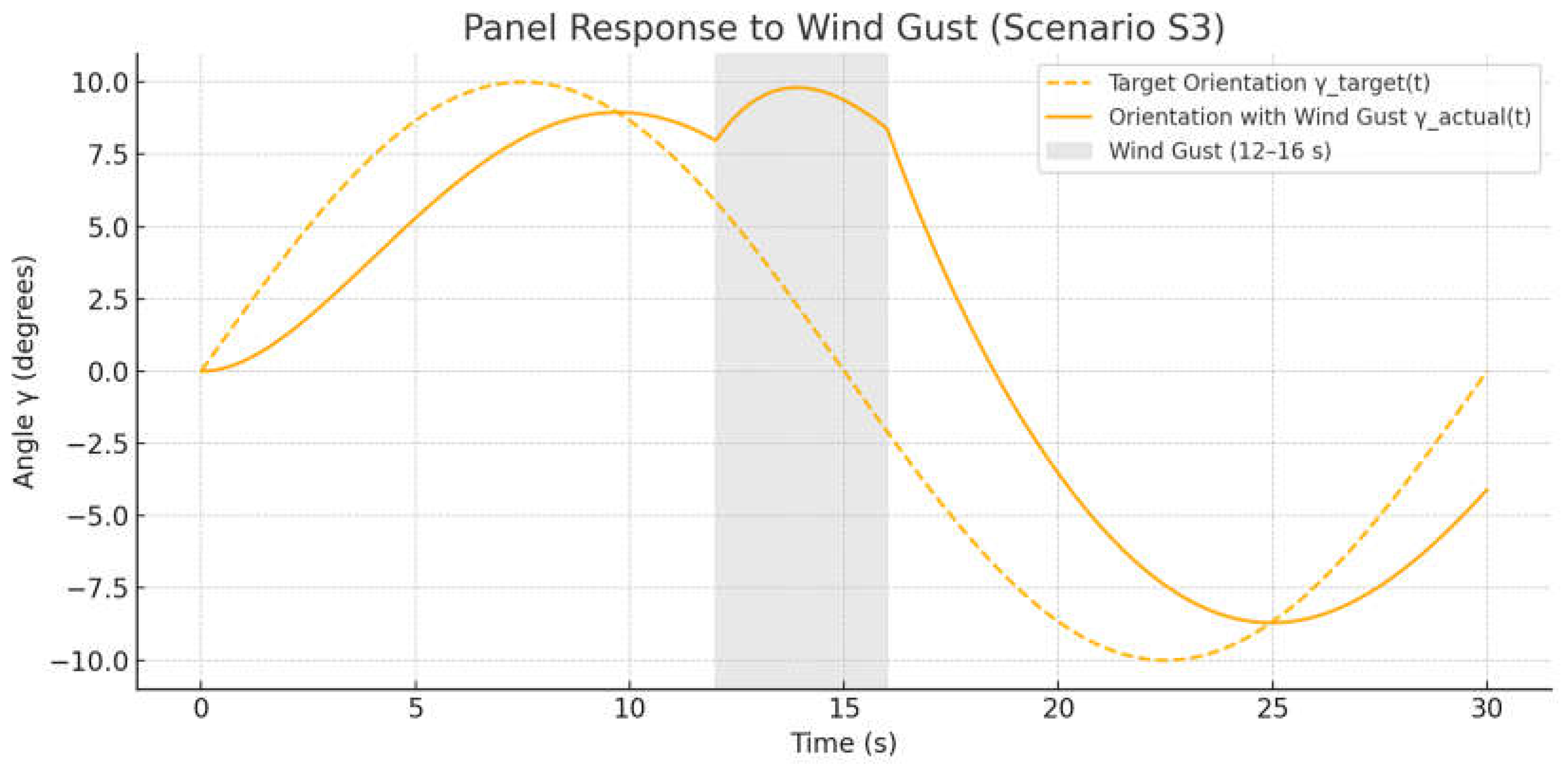
To assess the stability and reliability of the control system under real conditions, it was important to consider the impact of external disturbances, such as turbulence and wind gusts. Such phenomena can cause short-term spikes in aerodynamic torque, which disrupt the accuracy of panel orientation and increase the load on actuators. In this study (Scenario S3), a simulation was conducted to analyze the tracker’s response to a sharp wind gust within a limited time interval, with the goal of assessing the system’s ability to compensate for external disturbances without losing stability and with minimal tracking error.

Figure 7 shows the response of the solar panel under wind gust conditions (Scenario S3), where an external aerodynamic disturbance occurs in the time interval from 12 to 16 s, simulating a sudden increase in airflow. The yellow dashed line represents the target orientation trajectory γ_target(t) and the orange line shows the actual panel response γ_actual(t). The shaded area highlights the moment of the wind gust. It is evident that during this period, a noticeable deviation of the actual orientation from the target occurred: the amplitude of the response decreased and the delay increased. However, the system maintained stability—after the disturbance ended, the trajectory quickly returned to the target without signs of oscillation or self-oscillation. This demonstrates the correct response of the control algorithm to short-term external disturbances and its ability to dampen dynamic orientation disruptions.

Figure 8 shows the tracking error of the solar panel under short-term turbulence, corresponding to Scenario S3. The error is defined as the difference between the target and actual panel orientation angles $\epsilon \left(t\right)={\gamma }_{\mathit{target}}\left(t\right)-{\gamma }_{\mathit{actual}}\left(t\right)$. The time interval of the wind gust (12–16 s) is marked by the gray shaded area. During this period, a sharp drop in the error value was observed, down to −10°, reflecting an instantaneous loss of precise tracking due to the external aerodynamic disturbance. After the disturbance ended, the system demonstrated orientation recovery, but complete error suppression took a noticeable amount of time, indicating inertia and limited compensation speed from the actuator. Despite the significant error at the moment of disturbance, the behavior remained stable, without signs of self-oscillations or oscillations.

One of the key advantages of adaptive control is its ability to account for the current energy balance of a system. When the battery charge level decreases, it is critical not only to continue generation but also to minimize energy consumption, including reducing the panel’s deflection angles and aerodynamic load.

In Scenario S4, the tracker’s behavior was modeled during a gradual decrease in battery charge, resulting in the system automatically switching to an energy-saving mode. Figure 9 shows the behavior of the solar tracker with a decreasing battery charge. The yellow dashed curve represents the target orientation of the panel γ_target(t), formed without energy constraints. The blue dashed line displays the adapted control command, adjusted based on the battery state, while the green line shows the actual system response, the real panel orientation angle. It can be seen that as the battery charge decreased, the control system deliberately limited the panel’s deflection amplitude by reducing the rotation angle, which led to a decrease in both energy and mechanical loads. The actual trajectory closely followed the adapted command, demonstrating stability and consistency with the limitations imposed by the algorithm. This behavior confirmed the correct operation of the adaptation mechanism under conditions of energy deficiency.

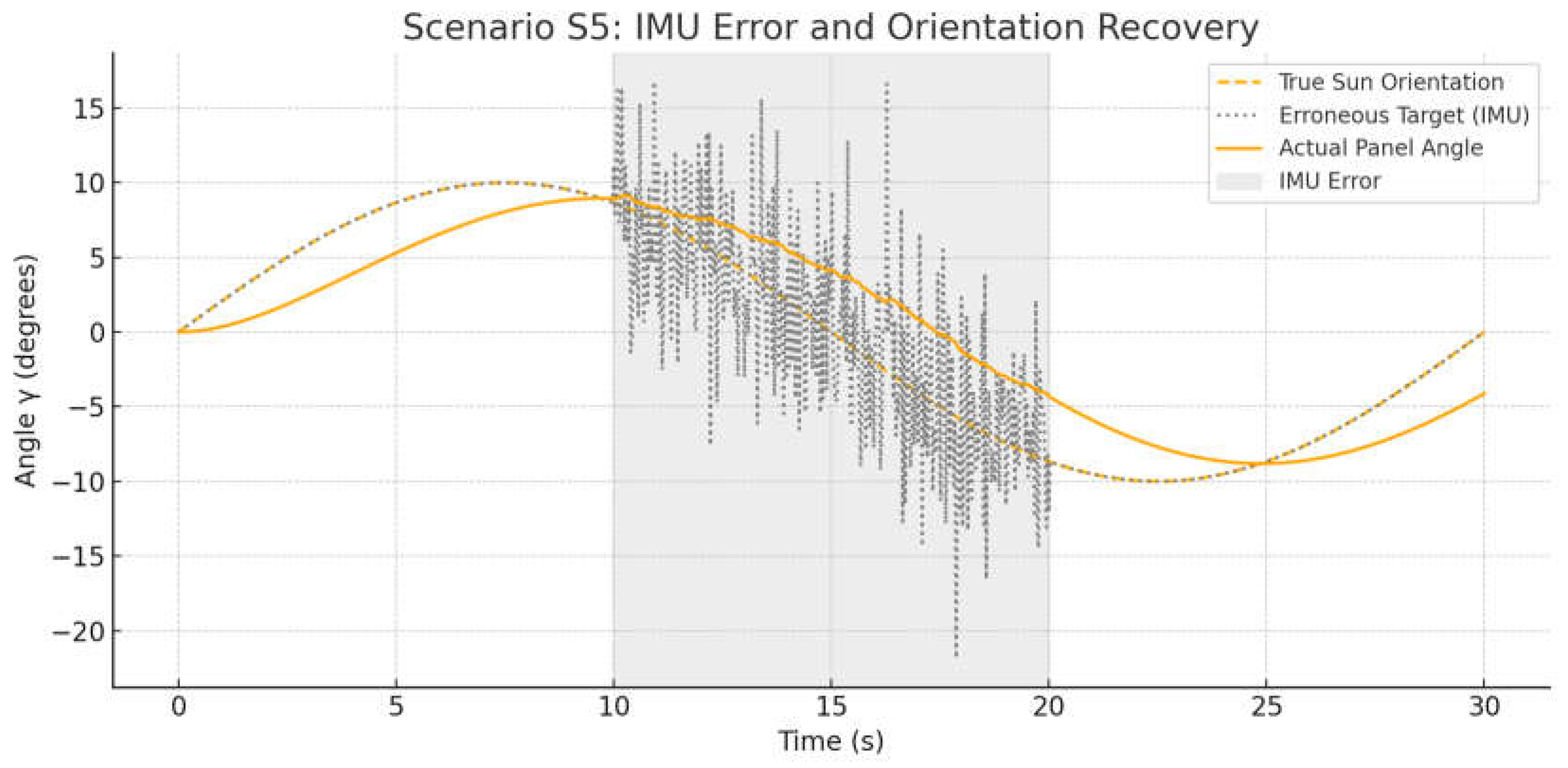
For real-time active control systems, the reliability of sensor data plays a crucial role. Errors in the readings of inertial measurement units (IMUs) can lead to the generation of incorrect control commands and, as a result, cause the panel to deviate from the true position of the Sun.

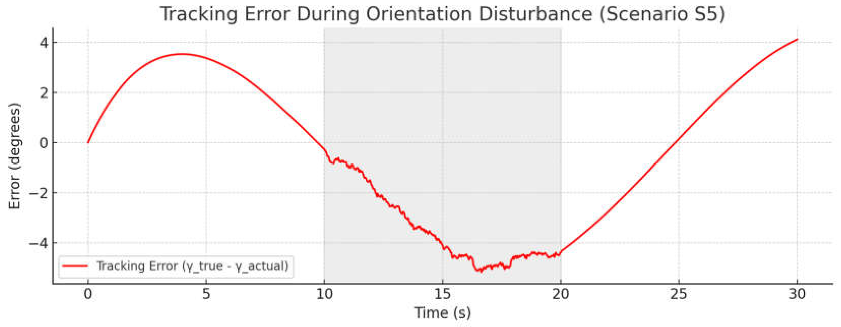
In Scenario S5, a situation was modeled where noise and errors were introduced into the orientation data coming from the IMU over a limited time interval. The goal was to assess the stability of the algorithm and its ability to recover after losing normal orientation perception. Figure 10 shows the dynamics of the panel’s orientation under sensor error conditions (Scenario S5) occurring in the interval from 10 to 20 s (marked by the gray shaded area). The yellow dashed line represents the true target orientation of the panel γ_true(t), while the black dashed curve represents the erroneous target command generated based on distorted IMU data. The solid orange line is the actual panel angle γ_actual(t), which deviated from the ideal during the sensor error period. During the sensor failure, fluctuations in the control command were observed, but the system demonstrated stability with limited deviation from the true orientation. After the distortion ended, the data stabilized, and the panel returned to the correct position. This confirmed the adaptive control algorithm’s ability to maintain controllability and compensate for failures when subjected to short-term distorted inputs.

Figure 11 shows the behavior of the solar panel orientation system when errors occurred in the inertial measurement unit (IMU) readings (Scenario S5). The blue line represents the true direction to the Sun, while the black dashed curve represents the erroneous target orientation calculated based on distorted IMU data. The orange line reflects the actual position of the panel, controlled based on the erroneous input. In the interval from 10 to 20 s (highlighted by the gray shaded area), a significant divergence between the true and target orientations was observed, caused by noise and fluctuations in the IMU. Despite this, the system maintained stability, with a limited level of deviation. After the distortion period ended, the system confidently restored the correct orientation, demonstrating the algorithm’s robustness to sensor failures.

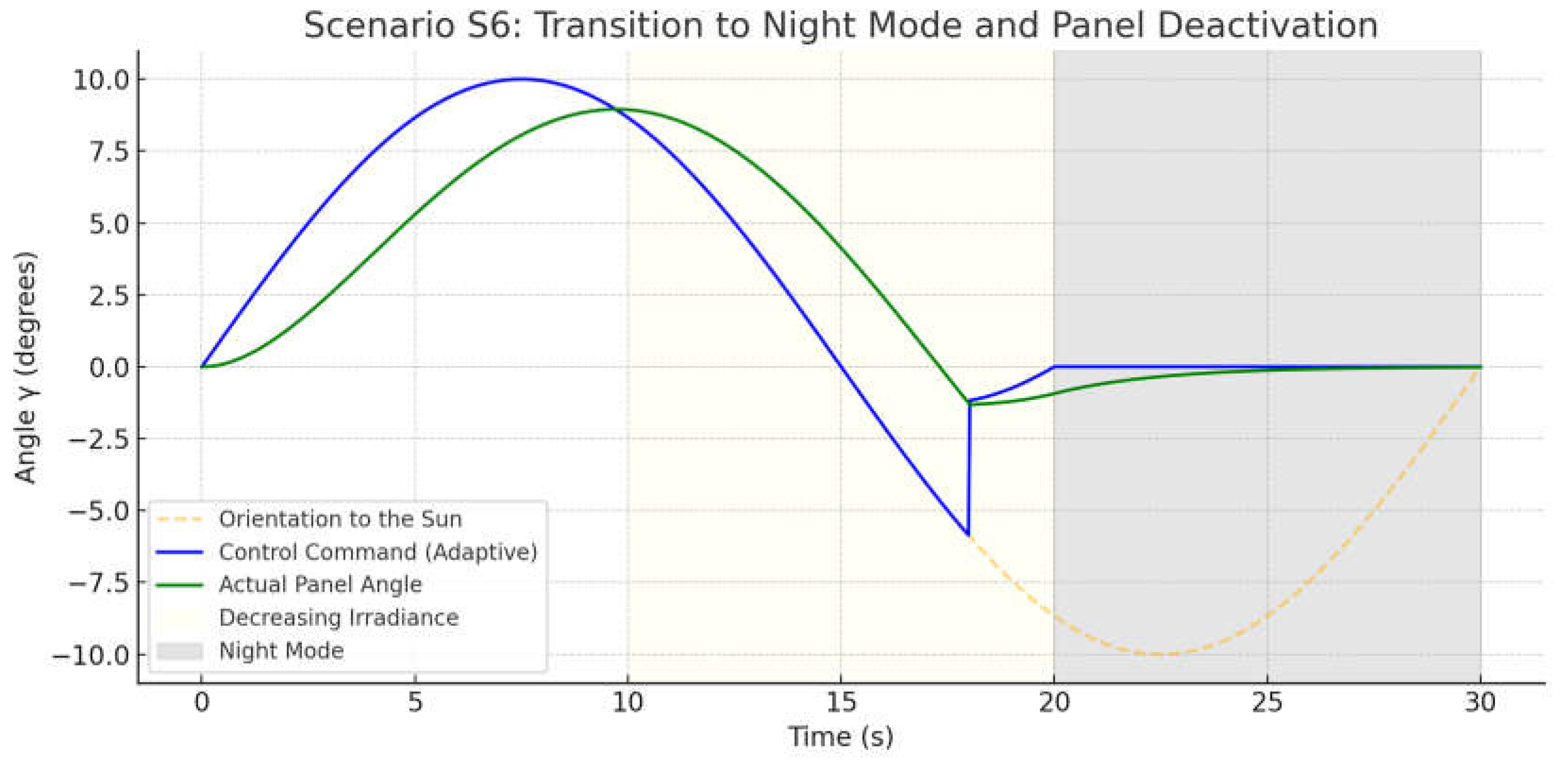
In conditions of decreasing illumination levels and the onset of nighttime, an unmanned aerial vehicle (UAV) should switch to a passive mode, disconnecting the panel from active tracking to avoid excessive energy consumption and load on the actuators. Scenario S6 simulated the behavior of the adaptive control system as the solar irradiance gradually decreased, leading to the transition into “night mode,” where the panel automatically positioned itself in a neutral position to minimize drag and conserve energy.

Figure 12 shows the behavior of the solar panel as the irradiance decreased and the system transitioned into night mode (Scenario S6). The yellow dashed curve represents the true position of the Sun, the blue line represents the adapted control command, and the green line shows the actual panel response. The light gray area (15–20 s) corresponds to the phase of decreasing irradiance, while the dark gray area (20–30 s) represents the night mode. As the light intensity decreased, the system adjusted the control input, gradually reducing the panel’s deflection angle. When the brightness reached a threshold value, the system automatically switched to night mode, and the actuator moved the panel to a neutral (zero) position. This demonstrated the correct implementation of the energy-saving logic: the system disconnects from active tracking when generating power is no longer meaningful, thereby reducing mechanical load and increasing overall efficiency.

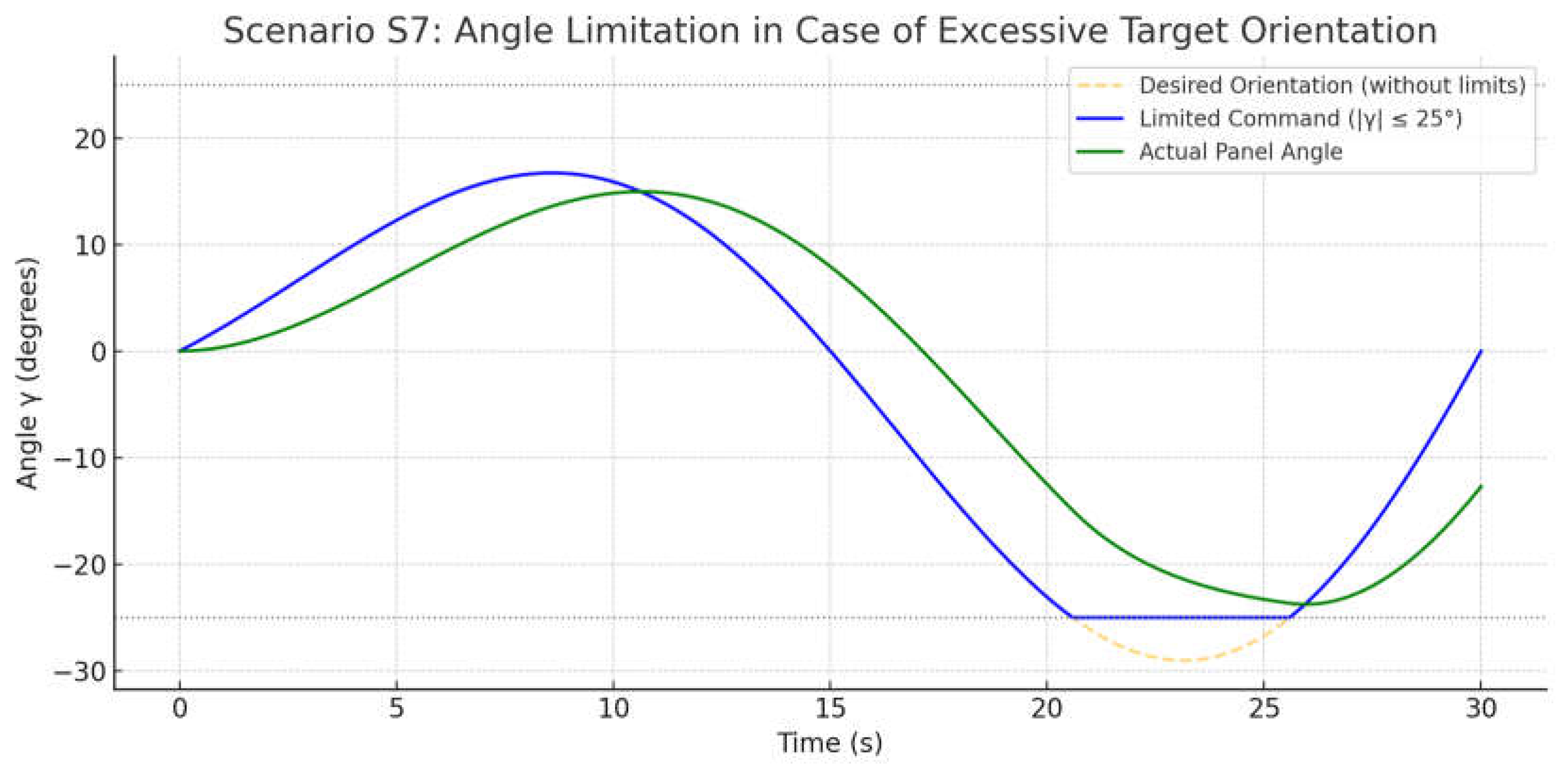
During panel orientation, the tracker may receive control commands that exceed the permissible deflection limits, which are constrained by aerodynamic and mechanical factors (angle γ > 25°). Exceeding these limits can lead to flutter, actuator overload, and reduced stability. Scenario S7 examined the behavior of the system with an intentionally increased target orientation of the panel and the operation of the maximum deflection angle limit.

Figure 13 shows the response of the solar tracker when the permissible deflection angle was exceeded (Scenario S7). The yellow dashed line represents the ideal (unrestricted) orientation toward the Sun, the blue line shows the limited control command with the condition ∣γ∣ ≤ 25°, and the green curve reflects the actual panel position. In areas where the desired orientation exceeded the structurally allowable limit, the control algorithm applied the limit, smoothly “cutting” the amplitude of the command. The panel accurately followed the limited signal, never exceeding safe values. This confirmed the correct implementation of the angular limitation mechanism, which protects the system from critical states and ensures reliable operation under extreme commands.

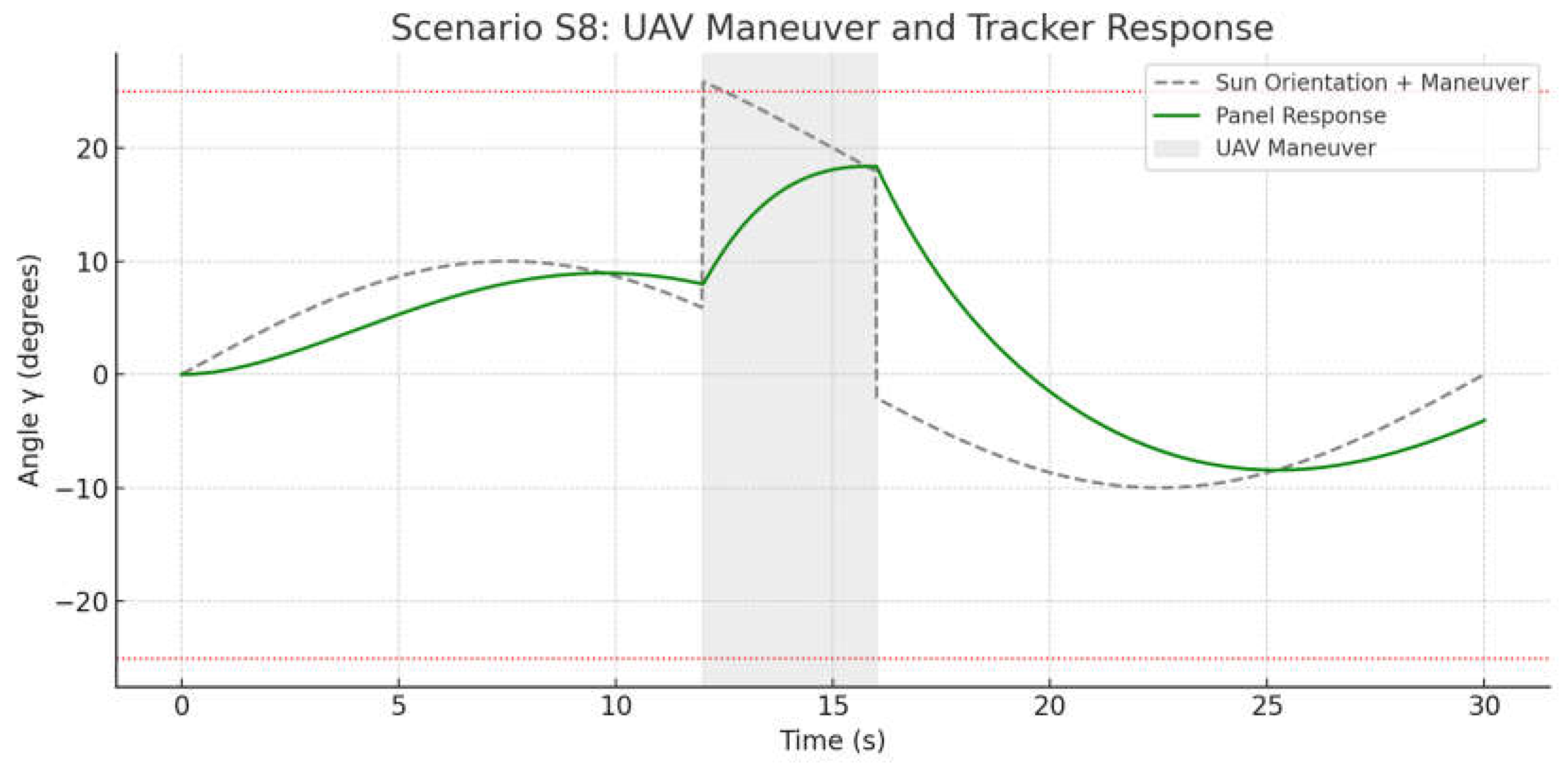
During active UAV maneuvers—such as sharp turns and changes in roll or pitch—the panel’s orientation relative to the Sun can change abruptly. In such conditions, the tracking system must correctly account for both the current position of the Sun and the movement of the UAV itself, adapting the control commands based on the platform’s dynamics. Scenario S8 simulates the response of the tracker to a brief UAV maneuver, accompanied by a sharp change in the orientation angle.

Figure 14 shows the solar panel response to the UAV maneuver (Scenario S8). The gray area (13–17 s) corresponds to the period of active maneuvering. The gray dashed line represents the resulting target direction (influence of the Sun + UAV movement), and the green line shows the actual panel position. It can be seen that during the maneuver, the target angle increased sharply, approaching the mechanical limit, indicated by the red lines. The tracker successfully responded to the change: the panel’s response remained within the permissible range and followed the main shape of the control signal without exceeding the limits. This demonstrated the system’s ability to adaptively and safely track the target direction, even during sharp movements of the platform.

In real flight conditions, multiple disturbances could occur simultaneously on the UAV—turbulence, energy transitions (e.g., night mode), and active maneuvers. To confirm the stability of adaptive control in complex scenarios, combined disturbances were simulated. In Scenario S9, the tracker’s performance was evaluated under the simultaneous action of a wind gust, UAV maneuver, and Sun direction change.

Figure 15 shows the behavior of the solar panel under the simultaneous influence of multiple factors (Scenario S9). The gray dashed line reflects the combined target orientation of the panel, incorporating the effects of the Sun, maneuver, and wind disturbance. The green line shows the actual panel angle.

The light gray area (12–16 s) corresponds to the UAV maneuver and the light blue area (15–19 s) represents the wind gust period. When the disturbances overlapped, the target angle increased and then became unstable due to turbulence. Despite the distortion of the input signal, the actual panel response remained within the permissible range, without signs of failure or instability. The system smoothed out sharp changes and demonstrated stable behavior under maximum load, confirming the reliability and adaptability of the proposed control algorithm.

The numerical experiments described in Section 4 confirmed the effectiveness and stability of the adaptive control algorithm for solar panel orientation under various external disturbances. In all nine scenarios (S1–S9), including ideal tracking, wind gusts, battery depletion, IMU errors, night mode, maneuvers, and their combinations, the system demonstrated correct behavior: it limited the amplitude, adapted the control input, and restored orientation without resonance. The adaptive strategy allowed the system to maintain energy generation while simultaneously reducing aerodynamic and mechanical loads. This confirms the practical applicability of the developed algorithm for unmanned platforms in real-world operational conditions.

In addition to improving angular alignment between the panel and the Sun, the implementation of an active tracking system introduces an energy trade-off that must be considered. On the one hand, better solar orientation increases incident irradiance and, hence, photovoltaic output. On the other hand, the tracking system consumes energy through periodic actuation and stabilization of the gimbal. While exact power consumption depends on the servo specifications and actuation frequency, the design aims to minimize control effort by maintaining panel orientation with short, infrequent adjustments. Moreover, the control algorithm includes a night-mode and energy-saving logic, which disables tracking when irradiance is low or when energy conditions are unfavorable. Qualitatively, simulations demonstrate that the energy gained through improved solar exposure outweighs the actuation cost under most daytime conditions, especially during long-endurance flights or variable sun angles. A detailed quantitative evaluation of the full energy balance, including real actuator consumption and power generation profiles, is planned as part of future experimental validation.

To summarize the behavior of the proposed tracking system,

Table 2. Summary of simulated scenarios (S1–S9) and control system response.

Scenario	Brief Description	Main Observations
S1	Ideal tracking	Panel follows Sun smoothly without overshoot or delay
S2	Fast change in Sun position	Temporary lag in alignment; panel gradually adjusts
S3	Wind gust applied	Minor angular deviation followed by successful stabilization
S4	Low battery condition	Panel movement is limited; power-saving mode activated
S5	Sensor noise/degraded IMU	Fluctuations in tracking; adaptive controller mitigates impact
S6	Transition to night mode	Panel moves to rest position; tracking deactivated
S7	Angular limits imposed (pitch/roll constraints)	Orientation respects aerodynamic limits; no violation observed
S8	UAV maneuver (sudden attitude change)	Panel compensates within allowed region; brief misalignment corrected
S9	Combined scenario (S3 + S4 + S5 + S6 + S7 + S8)	System adapts to multiple disturbances; tracking remains stable and safe

below presents a comparative overview of all nine simulated scenarios (S1–S9), as discussed earlier. These scenarios cover ideal tracking (S1), rapid Sun movement (S2), environmental disturbances (S3), energy limitations (S4), sensor degradation (S5), transition to night mode (S6), angular constraints (S7), UAV maneuvers (S8), and the combined scenario (S9). The table provides a qualitative summary of the system’s response in terms of tracking performance and control behavior.

Although the current study was primarily focused on numerical modeling and simulation, validation of the proposed control system is planned as part of future experimental work. The mathematical models used in this work, including the aerodynamic constraints and the adaptive controller logic, have been implemented in a simulation environment that reflects realistic UAV motion and solar trajectories. The response of the control system has been tested under a wide range of conditions, as summarized in Table 2. To ensure real-world applicability, future validation will include the following steps:

-

Construction of a physical testbed with a gimbal-mounted panel and programmable servos;

-

Measurement of real energy consumption during actuation cycles;

-

Use of a light sensor array or sun-tracking reference module for ground-truth comparison;

-

Evaluation of the control algorithm’s behavior in varying light and wind conditions;

-

Comparison of predicted and actual panel orientation angles and energy gains.

These steps will allow for a comprehensive verification of the model accuracy and controller performance. The integration of actual flight data from UAV hardware will also be explored to further validate the simulation assumptions.

6. Conclusions

This work was dedicated to the development, theoretical justification, and modeling of a three-axis adaptive solar tracking system designed for unmanned aerial vehicles (UAVs) operating under conditions of limited energy resources and external aerodynamic disturbances. Unlike traditional solutions focused on maximum solar tracking without considering the external environment, the proposed approach combines kinematic flexibility, physical–mechanical constraints, and adaptive optimization based on the system’s current state.

A key step in the process was the construction of a kinematic model for the panel orientation, which includes coordinate transformations from the inertial astronomical system (ECI) to the geographic system (FNED) and then to the UAV’s body frame coordinates. This model allows for the real-time, precise calculation of the direction to the Sun, taking into account the movement and position of the aircraft. Special attention was given to the aerodynamic analysis: using simplified empirical models, forces of resistance, lift, and torque arising from the panel’s deflection from the longitudinal axis were evaluated. This allowed for the quantitative determination of safe orientation limits, particularly the effective angle limit α ≤ 25°, driven by both mechanical and energy considerations.

The central element of the work was the development of the adaptive control algorithm, which minimizes not only the angular error between the panel normal and the Sun direction but also a generalized cost function that includes aerodynamic resistance, mechanical torque, energy generation, and weight factors that are adaptable based on the current battery charge and lighting conditions. This approach allowed for the implementation of an energy-saving orientation strategy that significantly reduces actuator load and aerodynamic drag without significant energy generation loss.

The numerical simulation covered nine operational scenarios, including both ideal and disturbed modes: sharp maneuvers, wind gusts, sensor degradation, battery depletion, and transition to night mode. In all cases, the system demonstrated stability, the correct adaptation of control inputs, and compliance with limitations. Notably, in combined scenarios with multiple overlapping disturbances, the algorithm maintained controllability and did not exceed critical torque or angle limits.

Thus, the proposed system combines theoretical rigor, physical realism, and practical applicability. The results are significant for the development of autonomous, resilient, and resource-efficient solar trackers for use in UAVs, satellite platforms, and other mobile energy systems. In the future, the work could be extended through experimental verification in flight tests, integration with real energy circuits, and optimization in multi-agent systems or group UAV operations.