Deterring Street Crimes Using Aerial Police: Data-Driven Joint Station Deployment and Patrol Path Planning for Policing UAVs

Abstract

Street crime is a critical public concern, attracting wide social and research attention. Conventional solutions to reduce street crimes are dispatching more police force in patrol and installing more cameras for street surveillance, which, however, suffer from huge manpower and financial consumption and limited performance. Inspired by the wide application of Unmanned Aerial Vehicles (UAVs) in policing and other related missions such as street surveillance, we investigate the use of UAVs in patrolling along high-risk streets to deter street crimes. UAVs significantly outperform police officers and street cameras in terms of cost reduction and deterring performance improvement. Technically, this paper proposes a data-driven framework to schedule the patrol UAVs, including an online patrol path planning module and an offline UAV station siting module. In the first module, the street-level deterring effect of the UAVs is estimated using a prediction-enhanced method, which guides the UAVs to patrol the high-risk streets more efficiently. Evolved from the path planning algorithm, the second module utilizes a data-driven method to estimate the deterring effect of the candidate UAV stations with different numbers of UAVs. Then both the location of the UAV stations and the UAVs at each station are determined. The proposed framework is comprehensively evaluated using a 6-year crime dataset of the Denver city. The results show that the proposed framework improves the deterring effect by 58.49% on average, and up to 157.32% in extreme cases compared to baselines.

1. Introduction

Crimes endanger human life, health and property. For example, there were 6 deaths by homicide per 100,000 (namely about 20,000 in total) of the population in the USA in 2019 [1]. A study [2] showed that more than 120 million violent crimes were committed in the USA yearly, resulting in a huge financial loss of almost USD 2.6 trillion. Among all the crimes, more than three-quarters are committed on the street, which will be verified with the 6-year real-world crime dataset of the Denver city. Street crimes occur in public and are typically characterized by violence or theft, including vandalism, car theft, mugging, assault, and drug-related offenses [3]. Thereafter, reducing the street crime rate is significantly critical to ensure public safety.

Currently, police departments mainly dispatch more police officers or install more street cameras to deter and reduce street crimes. Hochstetler et al. [4] studied the patrol planning strategy for police officers to minimize the police time-to-arrival and the overall number of patrol police officers. Multiple case studies [5,6] on the crime-deterring effect of police officer patrols demonstrate that increasing the police presence can effectively reduce the crime rate. However, onsite patrolling is mainly hindered by shortages of the police force, especially the available police officers, police cars, and patrol budget for police car maintenance, and fuel cost. For example, the number of police officers in the USA [7], Netherlands [8], and Canada [9] has been decreasing in recent years. Installing street cameras is another main method for street crime deterring. In New York City (NYC), about 25,500 cameras are employed for street surveillance, 3300 of which are publicly owned and in use by the government and law enforcement [10]. Some studies [3,11,12] on crime deterrence using cameras indicate that the cameras could partially reduce some crimes in some specific sites. However, the cameras show some serious limitations in deterring crimes. First, for a mega city such as NYC, there are tens of thousands of streets and avenues. As such, the cost of deployment, maintenance, and video processing (such as transmitting, storage, and criminal identification) of the cameras is huge. Second, the cameras can only record rather than respond to the crimes; thus, the effect of crime deterrence is limited. Therefore, the cameras cannot effectively reduce crime in these sites, such as around the city and town centers and public housing communities. Considering the serious problems caused by street crimes and the limitations of patrol police officers or street cameras in reducing street crimes, more cost efficient and effective methods are urgently needed to deter street crimes. With the development and proliferation of Unmanned Aerial Vehicles (UAVs), police departments are exploring UAVs for policing applications. For example, nearly half of the police departments in the USA have employed UAVs for law enforcement [13]. The UAVs could be equipped with police lights, policing alarms, or even non-lethal weapons (i.e., tear gas and rubber bullets [14]), and thus contribute to various policing-related applications such as area surveillance [15], target search and tracking [16,17], emergency material (i.e., medicine and first-aid kits) delivery [18], and even suspect neutralization with non-lethal weapons.

Therefore, this paper proposes and investigates deterring crimes using police UAVs to patrol along high-crime-risk streets, which outperform police officers patrolling and street cameras. Specifically speaking, policing UAVs is flexible and cheap, significantly saving policing resources/costs. Multiple UAVs can patrol the streets cooperatively, improving patrol efficiency. In addition, the mobility and response capability of policing UAVs make them deter crimes more efficiently than static cameras. With the obvious advantages of policing patrol UAVs, the paper conducts the first comprehensive investigation of patrol algorithm design for UAVs to deter street crimes. Specifically, this work aims to tackle two fundamental problems. The first one is how to plan the patrol path of the UAVs, considering both the temporal–spatial diversity of street crimes and the complexity of the street network of a given mega city. The second one is where to deploy the UAV stations and how many UAVs should be assigned for each station to maximize the patrol efficiency and deterrence effect under the limited flight range of the UAVs. By tackling these two problems, this paper contributes to the following four aspects:

• This work conducts the first comprehensive work on street crime deterring using the policing UAVs to patrol. A data-driven patrol framework with an online UAV patrol path planning module and an offline UAV station siting module is proposed to, respectively, tackle the two fundamental problems above.
• The online module introduces a multi-layer perception model to capture fine-grained spatiotemporal crime risks and extend classical submodular optimization algorithms [19,20] to handle multi-UAV coordination under routing constraints. The Prediction-Enhanced Greedy Algorithm (PGA) incorporates marginal reward functions to balance risk prioritization and energy efficiency, while the Prediction-Enhanced Evolutionary-Learning Based Algorithm (PEA) adapts genetic operators to optimize path diversity—addressing the critical challenge of scaling single-agent algorithms to multi-UAV systems, a limitation in the existing UAV patrol literature. We have found that in this problem, PEA performs well at a small scale (e.g., UAV count ≤ 5). However, as the problem scales to larger deployments (UAV count > 10), PGA demonstrates significantly better scalability and solution quality, attributed to its deterministic greedy selection mechanism that reduces computational overhead while maintaining deterrence coverage.
• In the offline module, a historical data-driven method is designed to estimate the deterring capacity of the candidate station locations and different numbers. The station siting and UAV assignment problem is modeled as a subset selection problem with UAV assignment constraints. A heuristic algorithm is leveraged to solve the problem, which allocates UAVs to stations with the highest deterrence coverage gain while satisfying physical constraints, bridging the gap between theoretical optimization and real-world deployment feasibility.

The remainder of the paper is organized as follows: Section 2 reviews the work closely related to this work. Section 3 introduces the datasets used in the work, conducts some preliminary analysis, and presents the problem and the solution framework. Section 4 introduces the online path planning module, followed by the offline UAV station siting module in Section 5. Section 6 presents the evaluation results. The conclusions of the work are drawn in Section 7.

2. Related Work

The work related to this paper can be divided into two categories.

2.1. Application of UAVs in Police and Other Applications

Being equipped with different on-board sensors, UAVs can achieve various tasks. For example, Bozcan et al. [21] and Trotta et al. [22] studied using UAVs for large-scale urban surveillance. Li et al. [23] developed a technology to enable UAVs to search targets in the dark (without visual light). Savkin et al. [24] proposed a UAV network navigation algorithm for optimal surveillance of a street target group. In a Global Positioning System (GPS)-denied environment, Vanegas et al. [25] designed a UAV visual-based algorithm for target finding and tracking. Furthermore, being equipped with actuators, UAVs can deliver parcels [26,27], which can be used in emergency item delivery in police [28].

Inspired by the remarkable various abilities of UAVs, police departments all over the world have introduced UAVs for police missions. Liu et al. [29] studied the South Korean police department to utilize UAVs for searching for missing persons. The protection of citizen rights such as privacy and transparency when using UAVs was also discussed. In 2020, the Baltimore Police Department implemented the Aerial Investigation Research (AIR) surveillance program to utilize the video surveillance of the city to support investigations for four different kinds of crimes including murders, non-fatal shootings, armed robberies, and carjacking [30]. The Canadian police department began to employ UAVs for various missions such as searching, locating suspicious items, and responding to disasters [31].

2.2. Crime Reduction

2.2.1. Police Patrol for Crime Reduction

Weisburd et al. [5] leveraged the police patrol and crime data in Dallas to show that a 10 percent increase in police presence at that location results in a 4.6 percent decrease in crime. A police patrol study in Philadelphia by Ratcliffe et al. [32] indicated that intensive patrol could increase the certainty of disruption and apprehension, which therefore reduced the crimes in urban areas. Nagin et al. [6] proposed the criminal opportunity model of offenders, which increased when the risk of apprehension declined. Using the one-year police patrol data from Minneapolis, Koper et al. [33] found that with enough police officers patrolling in high-crime-risk areas for enough time, crimes can be obviously deterred and reduced. A study in high-crime areas in three USA cities and two Colombian cities [34] showed that gun detection patrols in high-crime-risk areas can effectively deter gun crime. Blanes et al. [35] found that reducing the police response time can increase the likelihood of clearing the crimes and the likelihood that a suspect will be named by a victim or witness.

2.2.2. Deterring Crimes by Cameras

A 13-month test of the street cameras in Newark, NJ [3], showed that the auto thefts and shootings were significantly reduced after installing the cameras. Welsh et al. [11] found that the crime reduction at car parks was significant, which was nonsignificant at other locations such as city and town centers and public housing communities. Phillips et al. [12] conducted a comprehensive review of the studies evaluating crime reduction by cameras. The authors found that cameras could only effectively deter property crime. However, in some locations, cameras had little effect in reducing crimes. Ratcliffe et al. [36] studied the cameras’ deterring on crimes in Philadelphia, PA, USA. The research found that the cameras reduced the crime rate by only $13\%$, and cameras brought no crime reduction at a considerable number of sites. This is because the cameras could not move or respond to the crimes, so their deterring effect on the criminals is insignificant.

2.2.3. Crime Prediction

Precise crime prediction helps police officers and other stakeholders to prepare for the coming crime and may avoid the crimes and reduce the harm and cost of crimes. Brayne et al. [37] studied how crime prediction technologies impact the criminal justice processes and the perception of the criminal justice institution to the prediction technologies. Wang et al. [38] and Yi et al. [39] leveraged the spatial correlation, including region similarity or interaction, for more accurate crime modeling and prediction. Huang et al. [40] and Zhao et al. [41] leveraged the spatial–temporal correlation of urban crimes and multiple urban, mobile, and public service data for crime prediction. Zhao et al. [42] distinguished different types of crimes and captured the correlations among different types of crime and the spatial–temporal correlation of urban crimes for prediction. Zhang et al. [43] studied the interpretable machine learning algorithm for crime prediction, which can estimate the contribution of different factors to crimes. This work focuses on crime prediction within an ultra-wide urban area (wider than several km²) or long period (from days to weeks) due to the ultra-low crime frequency. Such a coarse-grained prediction can not be applied street-level patrol of policing UAVs.

2.3. Summary

The existing works reveal that increasing the police presence could effectively deter and reduce street crimes. However, the police resources (including the police officers, the policing vehicles, and the cost budget) are limited, which makes it hard to offer sufficient patrols for all the streets of a mega city. Street cameras suffer from a similar limitation of covering all the streets of a mega city. Moreover, the cameras could only record but not respond to street crimes and their deterring effect is insignificant.

Instead, policing UAVs are ideal instruments for street patrols to deter street crimes. Specifically, they are cheap, flexible, and easy to operate to replace police officers for street patrols. They can respond to crimes such as by delivering first-aid kits or even neutralizing the suspect with a non-lethal weapon, which could not only increase the deterring effect on street crimes but also decrease the response delay of the police. Even though policing UAVs show significant advantages in street patrol for crime deterrence, there have been few works on the patrol schemes until now, which is the motivation for this work.

3. Preliminary

This section first introduces the datasets employed to demonstrate the solution design, then conducts a preliminary analysis of the crime data to reveal the spatial–temporal dynamics of the crimes. Accordingly, the technical challenges of this work are presented. Finally, the solution framework is introduced.

3.1. Datasets and Preliminary Analysis

The basic information of the datasets, including the crime dataset, the street map, the contextual weather dataset, and the contextual points of interest (PoIs) dataset of Denver city, used in this work are summarized in

Table 1. Basic information of Denver datasets.

Dataset	Records	Area/km2	Period
Crime Dataset	3,837,250 Crimes	280.7	January 2016– December 2021
Contextual Weather Dataset	17,524 Records	280.7	January 2016– December 2021
Contextual POI Dataset	32,607 POIs	280.7	N/A
Street Map Data	207,457 Streets	280.7	N/A

.

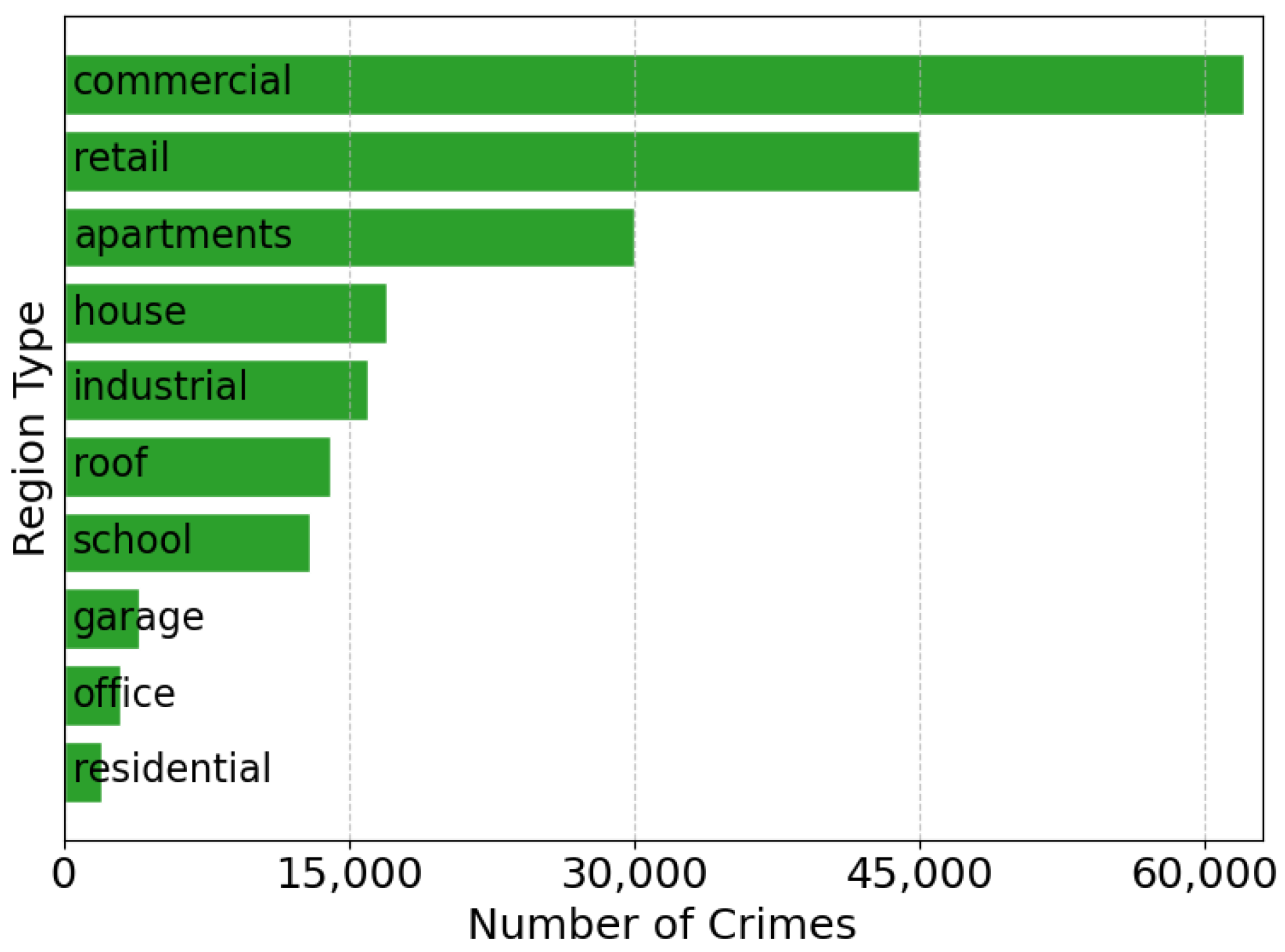
3.1.1. Crime Dataset

The criminal offenses dataset [44] in Denver city for the 6 calendar years (2016–2021) is used in this work, which is open-sourced by the National Incident-Based Reporting System (NIBRS). The dataset includes 3,837,250 crime records, each of which includes the ID, the occurrence time, the occurrence place, and thetype of a crime, as the field example in

Table 2. Field example of a crime record.

	ID	Type	Time	Location	Env.
Crime 1	2021224206	burglary	4/21/2021 17:17:00	−104.992, 39.733	Street
Crime 2	2021225054	theft	4/19/2021 10:02:00	−104.752, 39.653	In-home

shows. Amongst all the records, the ones with their environment fields include street-related keywords, such as “robbery-street” and “public-order-crimes-other”, are distinguished as street crimes. Finally, 3,167,250 street crimes are selected from the total crimes, the ratio of which is about $82.3\%$. Figure 1 demonstrates the spatial distribution of street crimes in the heatmap, with red indicating higher crime density and blue representing lower crime density.

3.1.2. Street Network

The street network of Denver was downloaded from OpenStreetMap [45]. According to the municipal information of Denver, the street map data within the area with the coordinates (lat = 39.6144, lon = −105.1099) as the south-west corner and coordinates (lat = 39.9142, lon = −104.6003) as the northeast corner are cropped as the patrol area of the UAVs, covering an area of around 280.7 km². Figure 2 shows the street network with the crimes on the street, where red-colored segments highlight streets with a higher frequency of criminal incidents.

3.1.3. Contextual Weather Dataset

The website [46] updates the weather conditions of the major cities of the world every half hour. To predict the occurring risk of the crimes, the weather contextual dataset during the same period of the crime dataset is crawled from the website. Each weather condition record consists of the weather, temperature, humidity, wind velocity, and air pressure. The total number of weather context records used in this work is over 17,524.

3.1.4. Contextual PoI Dataset

The PoIs, within the same area of the street map, are crawled from the OpenStreetMap [45]. Each building or infrastructure within the area is labeled as one of the following categories: leisure, commercial, tourism, healthcare, office, residential, study, or industrial. The total PoI record number of the entire area is 32,607. The PoIs of a region are encoded and combined with the contextual weather data as the feature for predicting the crime risk of a region. The city is partitioned into 1 km² square regions. For simplicity, a region is labeled as the same PoI if the number of PoIs is larger than other PoIs within the region. Figure 3 shows the total number of crimes in different regions.

3.2. Preliminary Analysis

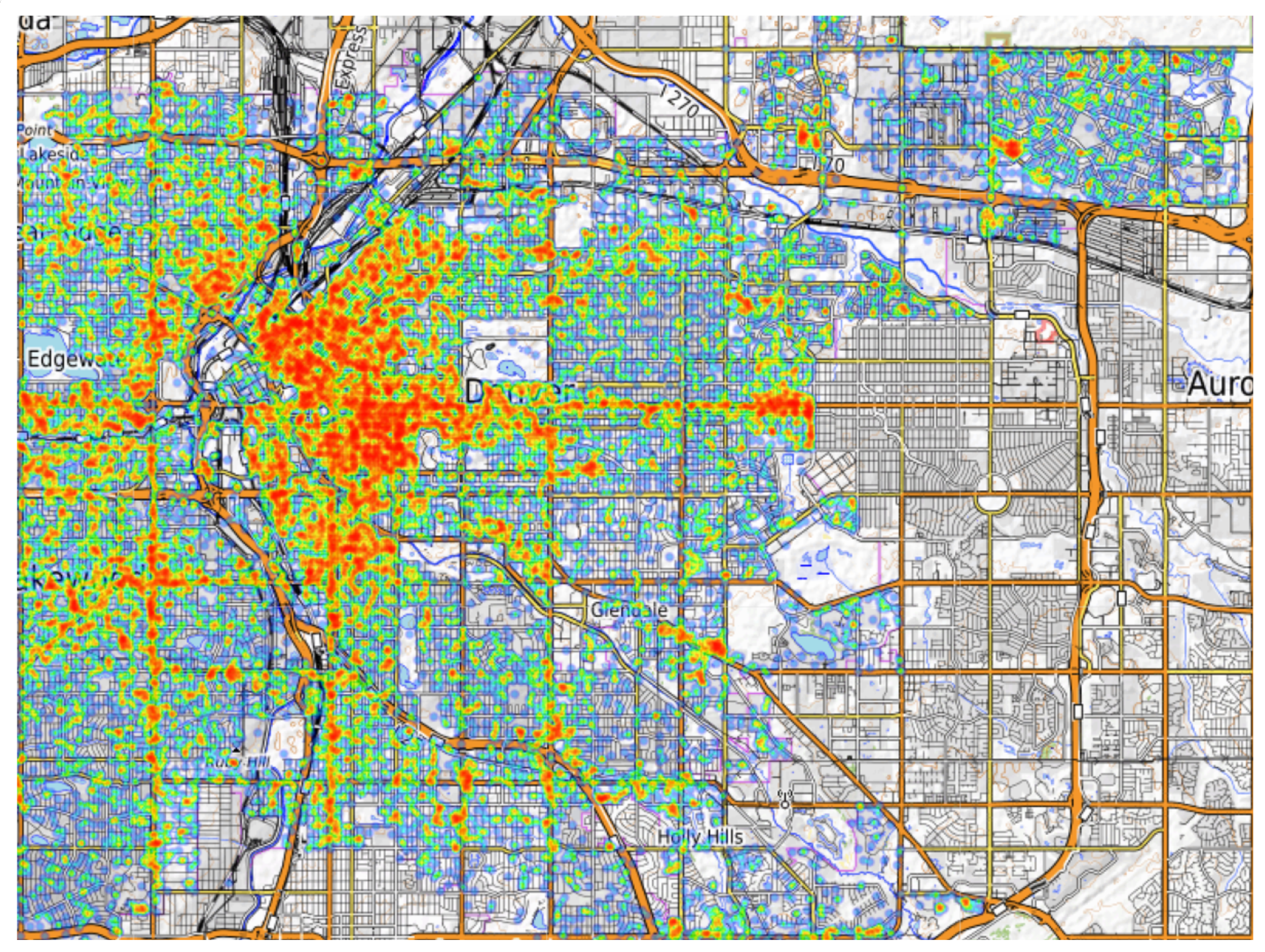
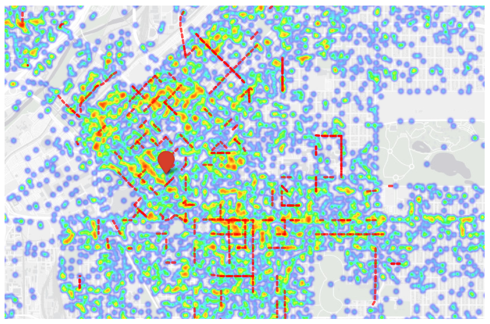
3.2.1. Spatial Distribution of Crimes

As shown in Figure 1, the urban commercial corridors and transit hubs are identified as the concentrated crime hotspots, with the crime density $3\times$ to $4\times$ higher than that of the residential zones. Figure 2 quantifies this spatial clustering, demonstrating that $45.34\%$ street crimes occur on the top $10\%$ of streets, which is tightly aligned with the commercial zones highlighted in Figure 1. The categorical breakdown in Figure 3 also agrees with this spatial logic, with the commercial districts ($32.7\%$) and retail areas ($13.6\%$) collectively contributing over $40\%$ of the total crimes. This indicates that the economically active PoI types dominate in shaping crime geography. Therefore, the algorithm for the module of patrol path planning should focus more on these high-risk commercial and retail areas to deter crimes effectively.

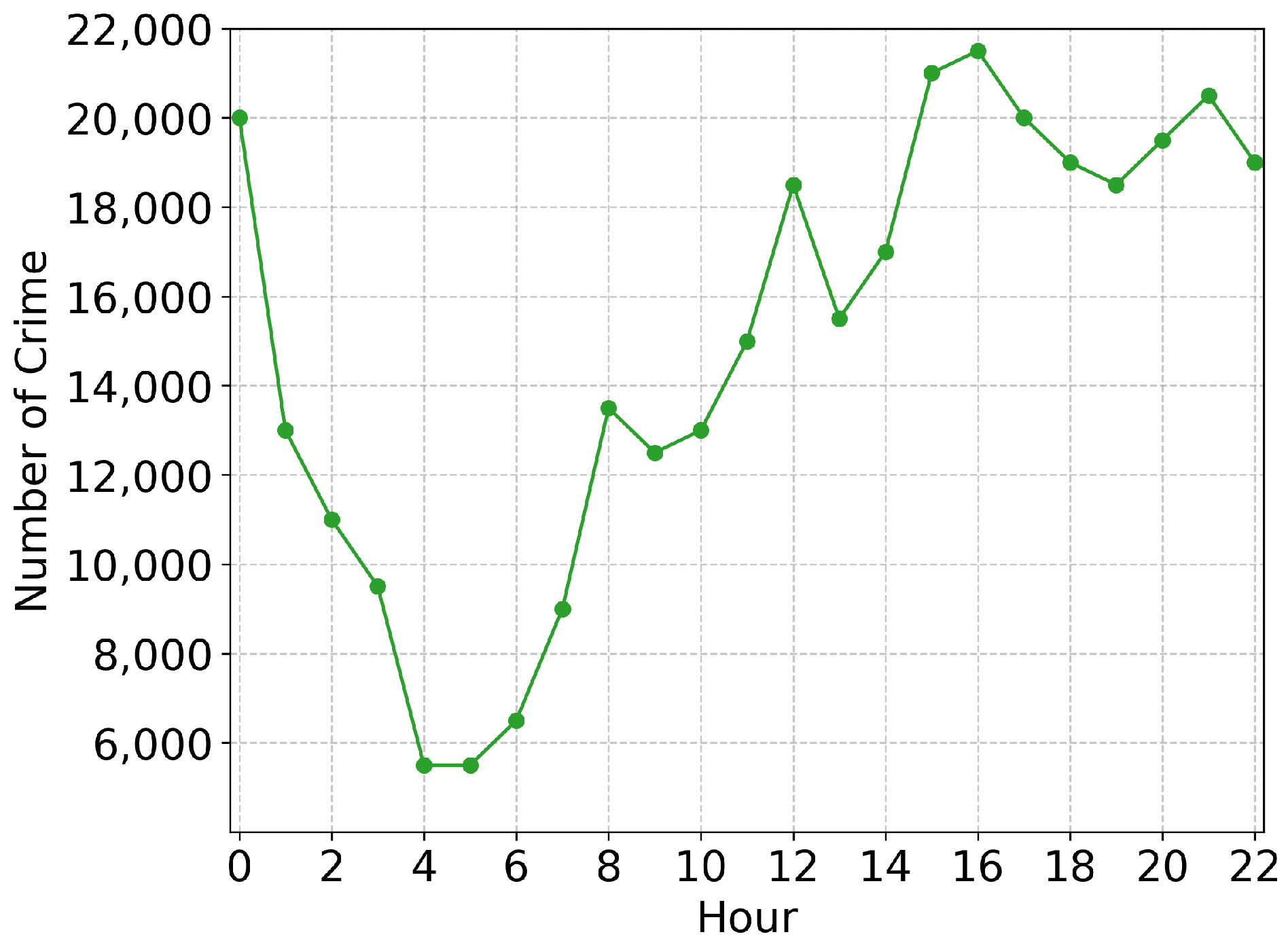
3.2.2. Temporal Distribution of Crimes

Temporal distribution of crime shows distinct circadian patterns. Figure 4 reveals that the crime incidence peaks at around 16:00 (with $14.2\%$ of the daily total) and troughs at around 05:00 (with only $2.1\%$ of the daily total). Notably, the 16:00–24:00 period accounts for $58.3\%$ of daily crimes, displaying a strong positive correlation with human activity patterns. This information is crucial for the deployment of UAV stations. Since most crimes occur during the afternoon and evening, the UAV stations should be strategically located to ensure that the UAVs can cover the high-risk areas during these peak crime times. The complementary CDF analysis in Figure 5 reveals a heavy-tailed distribution of the inter-crime intervals of the same street. In total, $50\%$ of the intervals exceed 1473 h (61 days), while only $15\%$ occur within 66 h, indicating both chronic and acute risk patterns. It suggests that the stations need to be able to respond to both sudden crime surges and persistent high-risk areas. The long-tail distribution of inter-crime intervals also highlights the need for an adaptive patrol strategy that can adjust to different risk levels over time.

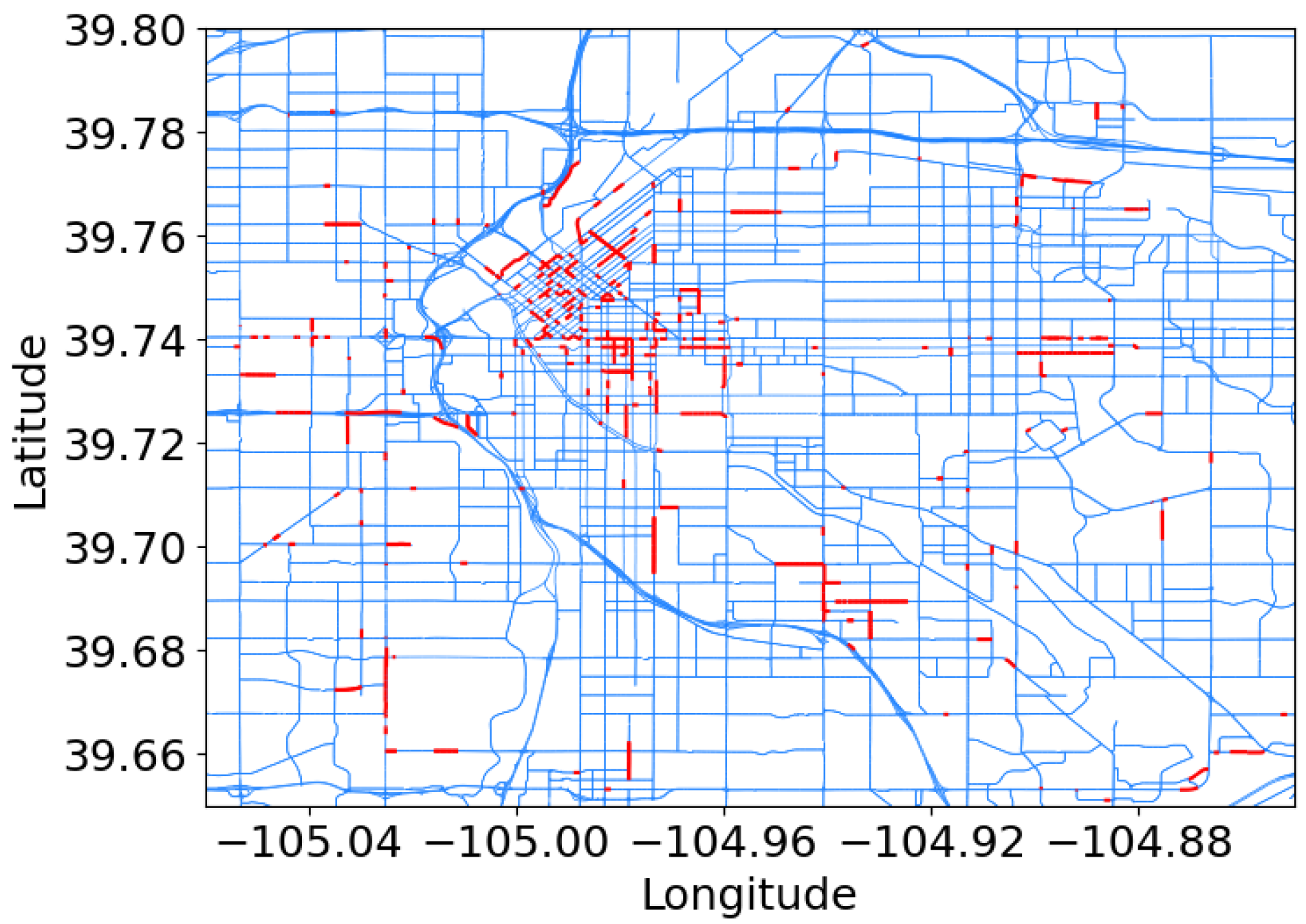
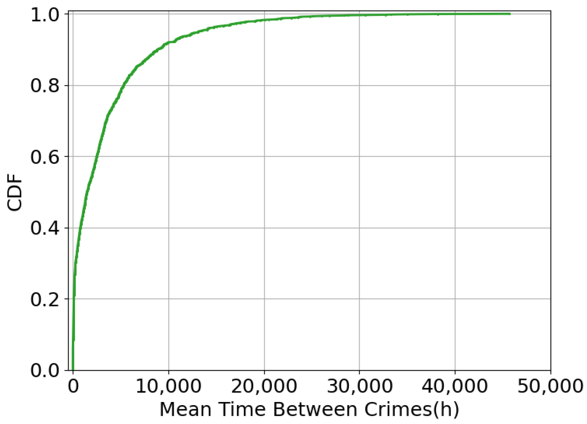
3.2.3. Relationship Between Street Length and Crime

There is a complex relationship between the length and the crime number of a street. Figure 6 demonstrates an unnoticeable relationship between the street length and the crime incidence. The data points are spread out, indicating variability in crime numbers across different street lengths. There is a noticeable concentration of points at shorter street lengths with varying crime numbers and fewer points as street length increases. This implies that simply considering street length is not sufficient for crime deterrence. Other factors such as the commercial PoIs surrounding the streets need to be considered for the patrol algorithm design. It also poses a challenge for developing UAV stations, as the stations need to be able to cover the streets of different lengths and crime patterns effectively.

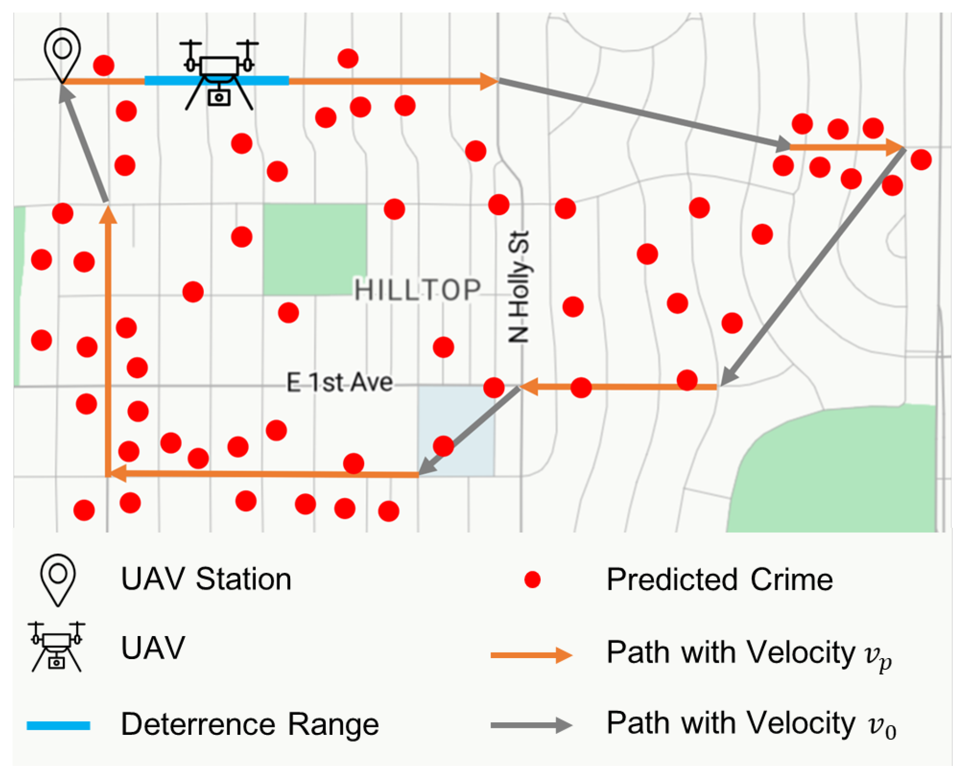
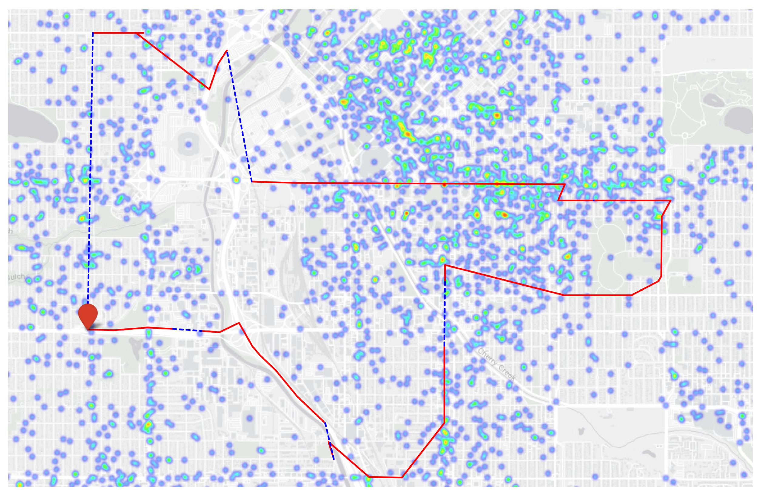
3.3. UAV Patrol Scenario and Problem Statement

A number of works [5,47,48] have been carried out on the deterring effect of police officers on crime. For example, the study by Weisburd [5] revealed that a $10\%$ decrease in police officers’ presence at a location results in a $7\%$ decrease in crime incidence, which is visualized in Figure 7. When the police officers’ presence time reaches around 5 min/h and 15 min/h, the crime risk falls to $44\%$ and $25\%$, respectively. Inspired by the work [5], this work assumes that the UAVs have a similar (but not necessarily the same) deterring effect on street crimes as patrol police officers. Studies have shown that police visibility significantly reduces crime rates, indicating that the perception of surveillance and risk plays a role in deterring criminal behavior [5,6]. While UAVs lack direct human interaction, they still serve as a strong visual signal of surveillance and potential intervention, which may influence offender behavior similarly to traditional patrols. While empirical field studies specifically measuring the exact psychological or behavioral response to policing UAVs are still limited, our assumption aligns with established theories of situational crime prevention and is supported by early practical deployments of UAVs in law enforcement [28,30,31].

To formally describe the patrol process and the deterring effect of the UAVs, the following two definitions are first presented:

Definition 1 

(Deterring Range, DR). The DR is the maximum distance from a UAV to a location so that the UAV can deter the crimes of the location. Let R denote the DR.

Definition 2 

(Effective Deterring Time, EDT). The EDT of a location is the shortest time during which a UAV is within the DR of the location so that the crime probability of the location can be deterred below a threshold. Let $t_0$ denote the EDT.

With the definition of DR and EDT, the typical patrol/deterring processes of a UAV are depicted in Figure 8, where red dots denote predicted high-risk crime locations, orange trajectories represent UAV paths patrolling at velocity $v_p$, and gray paths indicate rapid transit segments at maximum speed $v_0$. The blue shaded area delineates the UAV’s DR, within which crimes are effectively deterred during EDT. The UAV departs from its station (denoted by the station icon), prioritizes patrolling high-risk streets at $v_p$ to maximize deterrence coverage, and transitions to $v_0$ for inter-street patrol. The process of UAV patrolling is as follows:

• The UAV departs from its station after being fully charged;
• The UAV flies to a high-risk street with its maximum velocity $v_0$;
• After arriving at the street, it patrols along the street with the patrol velocity:

  $$v_p=min({\displaystyle \frac{2R}{t_0}},v_0),$$

  (1)

  where R is DR, $t_0$ is EDT, and the $min(,)$ operator guarantees that the deterring speed is smaller than the UAV’s maximum speed $v_0$;
• After deterring along the street, it seeks another high-risk street if its battery is sufficient, or returns to its station for energy replenishment if its battery is insufficient;
• It repeats the deterring process above to maximize the total deterring effect;
• When encountering unexpected events, UAVs are programmed to automatically alert the central dispatch center via real-time video/audio feeds and GPS coordinates and maintain overwatch of the incident area until ground units arrive.

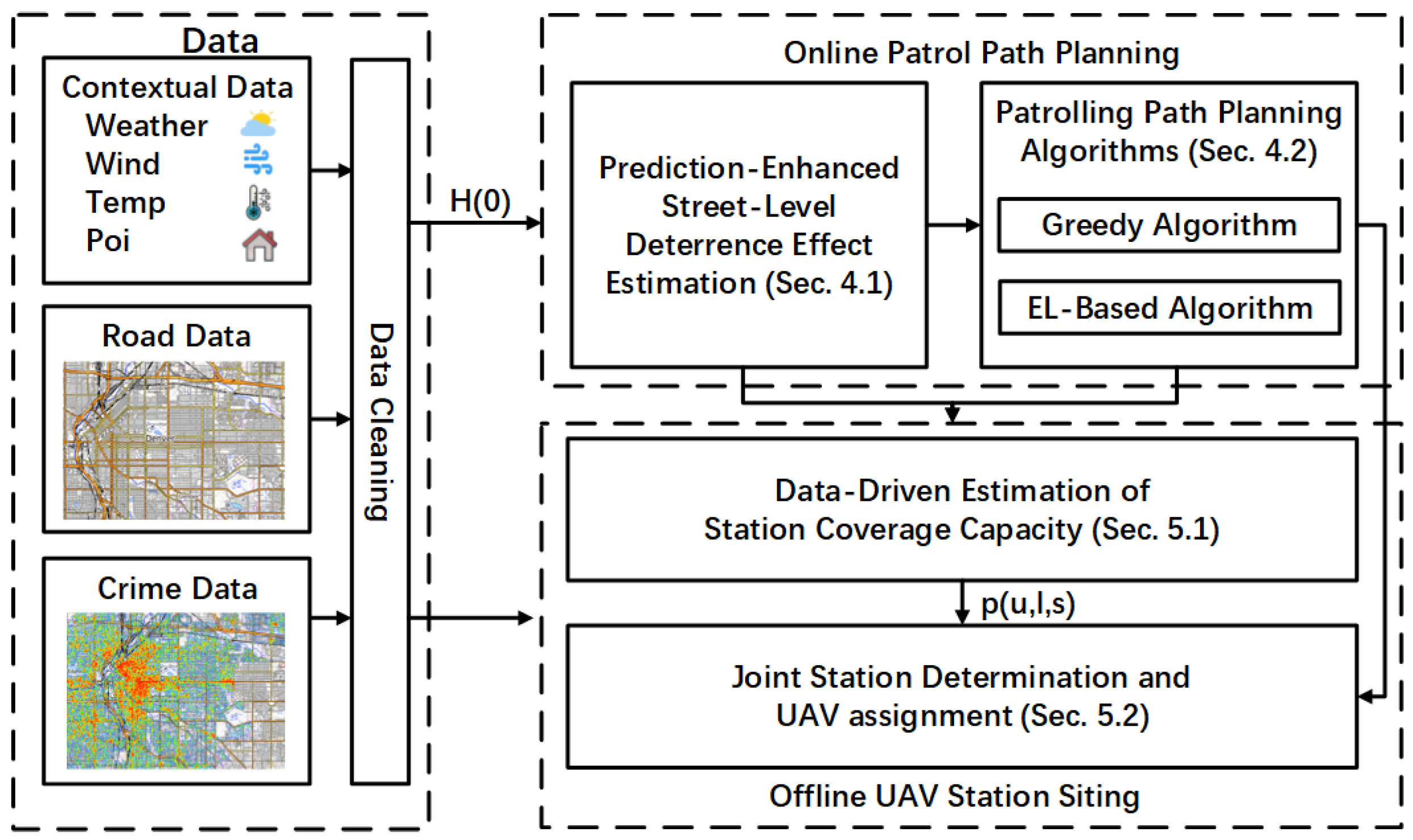
UAVs are not solely autonomous decision-makers but function as mobile cameras for law enforcement. UAVs complement—not replace—human officers. Their primary role is surveillance and deterrence, while direct intervention remains the responsibility of ground units. This design choice ensures that UAV path planning remains robust to short-term disruptions, as emergency responses are managed through established police workflows.

Considering the wide area of a mega city and the limited battery capacity of the UAVs, there should be multiple UAV stations and multiple UAVs, whose numbers are, respectively, denoted as L and U ($L\le U$). To maximize the deterring effect of the UAVs, the problems of this work include the following: (1) How should each UAV plan its deterring (flight) path during the patrol considering the constraints such as its available battery energy? (2) Where should the L UAV stations be deployed, and how should the U UAVs be assigned to each station?

3.4. Framework

To address the above problems, this paper proposes an innovative scheduling framework for thepolicing UAVs, as shown in Figure 9. The framework consists of three modules: the data module, the online patrol path planning module, and the offline UAV station deployment module.

3.4.1. Data Module

The data module serves as the foundational layer of the framework, responsible for preprocessing and structuring multi-source datasets input embedding for online and offline modules. The process begins with systematic filtering of missing or corrupted entries across crime records, weather data, and points of interest (POIs) to ensure data integrity. Subsequently, street-level crimes are spatially assigned to their nearest streets using Euclidean distance minimization [49], forming a crime weight matrix that quantifies street-level crime risk. To enhance analytical compatibility, categorical variables (e.g., POI types) undergo one-hot encoding, while temporal features (e.g., hour-of-day) are transformed via sinusoidal encoding to preserve periodicity. This preprocessing culminates in the generation of spatiotemporal crime risk maps, integrating road maps and historical crime statistics. These processed datasets are then standardized, ensuring a robust foundation for dynamic UAV patrol planning and station siting.

3.4.2. Online Patrol Path Planning Module

The online patrol path planning module operates under the assumption of pre-determined UAV station locations, focusing on optimizing patrol routes for UAVs by leveraging crime risk predictions and route-constrained subset selection. The module first designs a deep neural network (DNN)-based method to predict fine-grained street-level crime risk, integrating spatiotemporal features (e.g., time, weather) and contextual data (e.g., POI categories) from the data module. Then the UAV patrol path planning problem is formulated as a multi-subset selection task with routing constraints, aiming to maximize the deterrence of predicted crime risk while adhering to UAV flight time limits, which is solved by extending two different SOTA. By means of the UAV patrol path, the deterring capacity $p(u,l,s)$ is calculated as feedback for the offline station siting module, enabling iterative optimization of UAV deployment and station locations.

3.4.3. Offline UAV Station Siting Module

The offline UAV station siting module extends from the online path planning framework, determining optimal UAV station locations and UAV allocations through a data-driven approach. It leverages historical patrol coverage statistics from the online module to estimate the deterring capacity of candidate station sites under varying UAV numbers. By modeling the station siting and UAV assignment problem as a subset selection task with assignment constraints, a heuristic algorithm is designed to solve the problem. This closed-loop design ensures that station optimizations are informed by patrol feedback, enabling adaptive adjustments to UAV deployments and station layouts in response to evolving crime patterns.

4. Online Patrol Path Planning

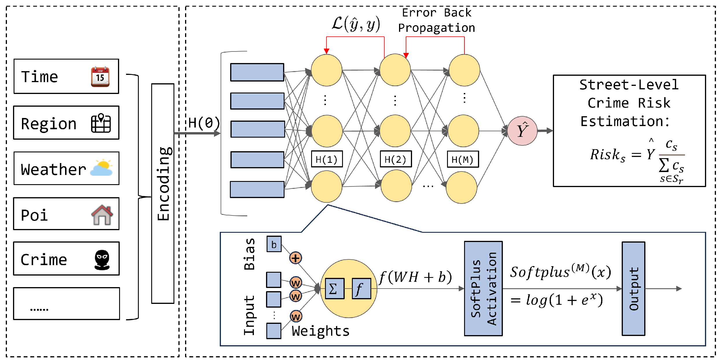
4.1. Prediction-Enhanced Street-Level Crime Risk Prediction

Some previous works revealed that both the weather condition and region functionality significantly impact the crime risk [38,42,50]. This work combines the above two features and some others, including season, date, and time for crime prediction. Let $\mathbb{R}$ represent the region set. Similarly, the time is divided into slots with equal periods (such as one hour). The prediction model is executed at the beginning of each slot to predict the crime number of each grid during the coming slot, which is leveraged to guide the patrol path planning of the UAVs. A multi-layer perceptron (MLP) [51], as a typical form of deep neural network (DNN), is leveraged to quantitatively capture the relationship between the contextual data and the crime data for prediction. The MLP is depicted in Figure 10, in which all layers are fully connected layers (FC layers), and each layer applies an activation function (AF). The fully connected layers are a type of neural network layer where each input node is connected to every output node. The activation functions are used to introduce non-linearity, allowing the neural network to learn complex patterns.

The first 5-year data are leveraged as the training data and the last 1-year dataset is leveraged as the validation dataset. Let M denote the number of the layers of the MLP and $H(j-1)$ and $H\left(j\right)$ denote the input and output of the j-th layer. Specifically, $H\left(0\right)$ is the input and $H\left(M\right)$ is the output of the MLP. The $\left|\mathbb{R}\right|$-dimension input $H\left(0\right)$ of the MLP is the crime number and the encoded contextual data:

$$H\left(0\right)={[\psi ,Time,Region,Weather,PoI]}^{\left|\mathbb{R}\right|},$$

(2)

where $\left|\mathbb{R}\right|$ is the total number of the regions; ${\psi }_r$ ($r\in \mathbb{R}$) is the crime occurring in the region r; Time indicates the time feature of crime; Region is the region ID ($r\in \mathbb{R}$); Weather includes the weather data (temperature, precipitation, etc.) at the time of crime $\psi$, and the PoI categorizes different areas (commercial, residential, etc.) of this region, providing insights into how POI affects the crime number. The computation of $H\left(j\right)$ ($j>0$) can be expressed as:

$$H\left(j\right)=f\left(W\right(j)·H(j-1)+b(j\left)\right),$$

(3)

where $W\left(j\right)$ represents the weight matrix of the j-th layer, $H(j-1)$ is the output from the former layer, and $b\left(j\right)$ is the bias vector for that layer. The function f denotes an activation function that introduces non-linearity into the model, enabling the neural network to learn complex patterns effectively.

To provide further technical details, the MLP architecture consists of an input layer, two hidden layers with 512 and 256 neurons, respectively, and an output layer. The hidden layers employ the ReLU activation function to mitigate vanishing gradient issues, while the output layer uses the Softplus function (as defined in Equation (5)) to ensure non-negative crime risk predictions. The model is trained using the Adam optimizer with a learning rate of 0.001 and a batch size of 64. Dropout regularization (rate = 0.3) is applied after each hidden layer to prevent overfitting. The training process spans 200 epochs with early stopping based on validation loss convergence. These hyperparameters were selected through grid search to balance predictive accuracy and computational efficiency.

To evaluate the prediction loss of the MLP, the MSE Loss is used as the loss function, which is defined:

$$\mathcal{L}(\widehat{y},y)={\displaystyle \frac{1}{m}}\sum _{i=1}^m{({\widehat{y}}_i-y_i)}^2,$$

(4)

where ${\widehat{y}}_i$ indicates the predicted value for the (i)-th sample, $y_i$ is the true value for the i-th sample and m represents the total number of samples in the dataset.

The predicted result is expected to be non-negative, so the Softplus activation function is used as the final activation function, which is defined as:

$$Softplu{s}^{\left(M\right)}\left(x\right)=log\left(1+e^x\right).$$

(5)

The predicted crime number matrix all of these regions ($\mathbb{R}$) is:

$$\widehat{Y}=W\left(M\right)·H(M-1)+b\left(M\right),$$

(6)

where M denotes the index of the final output layer. Let ${\widehat{Y}}_r$ represent the predicted crime number of region r during the coming time slot, ${\mathbb{S}}_r$ denote the street set within the region r, and $c_s$ denote the total crime number of the street $s\in {\mathbb{S}}_r$. Then the crime risk $Ris{k}_s$ of each street s during the following time slot is:

$$Ris{k}_s={\widehat{Y}}_r{\displaystyle \frac{c_s}{{\sum }_{s\in {\mathbb{S}}_r}{c}_s}}.$$

(7)

4.2. Patrol Path Planning Algorithms

The patrol path planning problem for a single UAV with limited battery capacity is to maximize the total deterred crimes of the street subset among the street set, with its limited flight time/range. This problem refers to the well-known subset selection problem with routing constraint [19], which is a single-subset selection problem with constraint problem and referred to as a single-UAV problem for simplicity. In the problem, a street is an element of the set, the crime number of a street is the reward of the street, the time patrolling the street is the selecting cost, the time transferring among two streets is the edge cost, and the routing constraint is that the total flight time should be shorter than the available flight time of the UAV. One technical challenge of the problem is that the cost function is not deterministic but approximate (for example by a walk through a graph passing all nodes). Some existing works [19,20,52] designed several remarkable algorithms for the single-subset selection problem. Specifically, Zhang et al. [19] proposed a greedy algorithm with a provable approximation guarantee. Inspired by the work of Zhang et al. [19], Chao et al. [52] and Bian et al. [20], respectively, proposed an Evolutionary Learning (EL)-based algorithms, which may outperform the greedy algorithm [19] with a longer learning time. To summarise, the greedy algorithm is more deterministic, which may be stuck into local optima, while the EL-based algorithm may find a better solution because it learns globally, at the cost of execution time.

This paper studies the scheduling of multiple UAVs for crime deterrence, whose objective is to find a path for each UAV to maximize the number of total deterred crimes by UAVs under their energy and flight range constraints. This is denoted as a multi-subset selection problem with routing constraint and referred to as a multi-UAV problem for simplicity. The algorithms for the single-UAV problem could not be directly applied. Then, the greedy algorithm [19] and the EL-based algorithm [52], are, respectively, extended to the multi-UAV problem, whose performance is thereafter comprehensively compared.

4.2.1. Greedy Algorithm

In the greedy algorithm [19], the greedy principle is to find the street with the maximum marginal reward (maximum crime number/flight time) in each iteration until all streets are scheduled to patrol or the flight range constraint is violated. The street maximum marginal reward is represented as:

$$s^{*}=arg\underset{s\in \mathbb{S}}{max}{\displaystyle \frac{Ris{k}_s}{\mathsf{\Delta }Rout{e}_s}},$$

(8)

where $Ris{k}_s$ is defined in Equation (7) and $\mathsf{\Delta }Rout{e}_{s,u}$ is the cost of selecting s (namely the total time to fly to and patrol along the street s). The routing of a UAV can be planned by the existing heuristic algorithms [19]. In the multi-UAV case, the greedy principle in each iteration is to select the street to the UAV with the maximum marginal reward for any UAV u,

$$s_u^{*}=arg\underset{u\in \mathbb{U},s\in \mathbb{S}}{max}{\displaystyle \frac{Ris{k}_s}{\mathsf{\Delta }Rout{e}_{s,u}}},$$

(9)

until all streets are selected or the routing constraint for all UAVs is violated. For each selected street, it will be removed from the street set $\mathbb{S}$ to avoid repeat calculation on street-level crime risk $Ris{k}_s$. Notably, in the multi-UAV scenario, each UAV’s decision is shared across the entire fleet of UAVs. Once a street is assigned to a particular UAV, it cannot be assigned to another UAV, ensuring the patrol of each street by only one UAV. This prevents overlap in patrol routes and ensures efficient deterrence. However, with multiple UAVs, additional constraints are considered in the optimization process, such as keeping each UAV working within its flight time limitation and the total patrol time under the limitations across all UAVs. The routing adjustments made in the multi-UAV scenario also account for the need to efficiently distribute the patrol duties among the UAVs, ensuring the assignment of each UAV to a set of streets that collectively maximizes the deterring effect while minimizing the operational costs. However, with multiple UAVs, additional constraints are considered in the optimization process, such as ensuring that no UAV exceeds its flight time and that the total patrol time is under the limitation across all UAVs. The routing adjustments made in the multi-UAV scenario also account for the need to efficiently distribute the patrol duties among the UAVs, ensuring that each UAV is assigned a set of streets that collectively maximizes the deterring effect while minimizing the operational costs.

4.2.2. EL-Based Algorithm

This work also implements the EL-based algorithm for the multi-UAV scenario, inspired by the EL-based algorithm for the single-UAV problem. The EL-based algorithm consists of chromosome initialization, selection, crossover, and mutation:

• Chromosome Initialization: To improve the efficiency of the search process, the initialization is performed using a weighted probability approach. Each street is assigned a weight based on its crime risk, which is divided by its distance from the initial point of the UAV’s flight path. The higher the weight, the higher the probability that the street will be selected to form a part of a patrol path of a UAV. This heuristic ensures that streets with high crime risk and those closer to the initial point are more likely to be selected, guiding the algorithm towards streets that could have a higher crime risk.
• Selection: The quality of a patrol path for each UAV is estimated using a fitting function, which takes into account both the crime risk and the length of the streets along the path. The fitness function is defined as:

  $$fitness\left(c_u\right)=\sum _{s\in c_u}{\displaystyle \frac{Ris{k}_s}{Lengt{h}_s}},$$

  (10)

  where $Ris{k}_s$ is the crime risk of street s from chromosome path $c_u$ and $Lengt{h}_s$ is the length of that street. The selection step involves choosing the Top-$\left|U\right|$ patrol paths $c_u$ with the highest fitness values. These paths are the most promising candidates for the next generation of patrol routes.
• Crossover: In this step, the streets of two selected parent paths are combined to produce new offspring paths. To introduce diversity into the population and prevent premature convergence, a heuristic method is applied during the crossover process. Two streets are randomly selected from the parent paths. If the distance between these two streets is smaller than a given threshold, they are chosen for a single-point crossover. If the distance is greater than the threshold, a new pair of streets is selected, and the process is repeated. This ensures that the crossover is meaningful in terms of the geographical proximity of the streets being combined, which enhances the practicality of the generated paths.
• Mutation: For each newly generated patrol path, each street may be subject to mutation with a certain probability. If a street is selected for mutation, it is replaced by a nearby street, where the replacement is made within a specified distance threshold. After the mutation, the fitting function of the new path is recalculated to evaluate its quality. The mutation step introduces further diversity into the population, allowing the algorithm to explore a wider search space.

These steps are repeated until a stopping criterion is met (e.g., a maximum number of generations). The algorithm generates an optimal patrol path for a single UAV. Each UAV in the fleet runs the EL-based algorithm independently, generating its own patrol path. Importantly, during this process, each UAV’s path is planned while excluding streets that have already been assigned to other UAVs, ensuring that there is no overlap in patrol routes.

In the multi-UAV scenario, each UAV utilizes the EL-based algorithm to plan its patrol path independently. After each UAV has independently generated its path, a coordination phase occurs where streets already selected by other UAVs are excluded from consideration for new UAVs. This ensures that each UAV operates within its assigned region without redundancy. Additionally, in this multi-UAV framework, the number of UAVs influences the diversity of the population and the exploration of the solution space. With more UAVs, the algorithm can explore more patrol paths, as the population of candidate paths increases. However, this also requires that the algorithm balance the distribution of streets across UAVs while considering their operational constraints (e.g., flight time). Thus, the objective is not only to generate high-risk patrol paths for each UAV but also to optimize the overall coverage of the area, with each UAV covering a distinct set of streets. Overall, the multi-UAV EL-based algorithm provides a scalable and efficient solution for patrolling large areas, leveraging both evolutionary principles and heuristic methods to improve search efficiency in the solution space and optimize patrol effectiveness across multiple UAVs.

5. Offline UAV Station Siting

For clarity, the main notations used in the remainder of this paper are summarized in

Table 3. Notion.

Parameter	Description
R	DR
$t_0$	EDT
$v_0$	Effective deterring Velocity
$v_m$	Maximum Velocity
X	Street Crime Number
l()	Street Length
T	Maximum Flight Time

.

5.1. Data-Driven Estimation of Station Deterring Capacity

The station coverage capability quantifies the deterring effect of the UAVs from a candidate station location to the surrounding streets. The metric $p(s,l,u)$ denotes that the probability of a street s is deterred by the station l with u UAVs. A data-driven method is leveraged to estimate $p(s,l,u)$ using the patrol path planning algorithm in the last section. Specifically, given the datasets, the patrol path planning algorithms could be executed within the period of the training dataset, and $p(s,l,u)$ could be obtained. Taking a randomly chosen coordinate $(-104.99,39.75)$ as an example of a candidate station, Figure 11 visualizes both the heatmap of the crimes during the period of 2021 and the deterred streets of five UAVs from the station with a greedy algorithm. The background heatmap employs a gradient from red to blue, where red zones denote areas with high crime density, reflecting historical crime hotspots. Overlaid on this heatmap, dashed red lines represent the patrol paths of five UAVs, strategically routed to prioritize coverage of high-risk streets (coincident with the densest red regions). And the red pin icon marks the UAV station location. This figure shows that the deterred streets partially overlap with the high-risk streets. This is because the path planning algorithm does not always choose the street with the highest risk to deter (see Equation (9). This shows the path planning algorithm could balance the deterred crimes and the deterred range to a certain degree.

Figure 12 numerically illustrates the $p(s,l,u)$ for the West 32nd Avenue (s), in which the X-axis is the UAV number and the Y-axis is $p(s,l,u)$. When the UAV number is smaller than 10, $p(s,l,u)$ increases nearly linearly, while when the UAV number is larger than 10, $p(s,l,u)$ increases much slower. When the UAV number reaches 40, $p(s,l,u)$ approaches 1. Figure 13 numerically illustrates the average $p(s,l,u)$ for all the surrounding streets of the example candidate station location, which shows that the UAV number has a significant influence on $p(s,l,u)$. With more UAVs being deployed, the probability of street coverage increases.

5.2. Joint Station Determination and UAV Assignment

To formulate the problem of the station siting and UAV assignment problem, several notations are introduced. Let the set $\mathbb{X}\in \mathbb{L}$ denote the set of the chosen locations for the UAV stations. Let the set $U_{\mathbb{X}}=\left\{u_l\right|l\in \mathbb{X},{\sum }_{l\in \mathbb{X}}{u}_l=U\}$ denote the number of the UAVs assigned to the sited stations, whose total number is U. Since one street may be deterred by the UAVs from multiple stations. The deterring effect of multiple stations to a single street by multiple stations is estimated as $1-{\mathsf{\Pi }}_{l\in \mathbb{X}}(1-p(u_l,l,s))$. With the estimation of the deterring capacity ($p(s,l,u)$) of any candidate station location and the notations, the problem is formally formulated as:

$$\begin{array}{cc}\hfill max& Cover(U,\mathbb{X})=\sum _{s\in \mathbb{S}}[1-{\mathsf{\Pi }}_{l\in \mathbb{X}}(1-p(u_l,l,s))]\overline{c_s}\hfill \end{array}$$

(11)

$$\begin{array}{cc}\hfill \mathrm{s}.\mathrm{t}.& \mathbb{X}\subseteq \mathbb{L},\hfill \end{array}$$

(12)

$$\begin{array}{cc}\hfill & \left|\mathbb{X}\right|\le L,\hfill \end{array}$$

(13)

$$\begin{array}{cc}\hfill & \sum _{l\in \mathbb{X}}{u}_l=U.\hfill \end{array}$$

(14)

The problem is explained as follows: $Cover(U,\mathbb{X})$ in Equation (11) is the objective function, which maximizes the total deterring effect of the sited UAV stations and the assigned UAVs; $\mathbb{X}$ in Equation (12) is the optimization variables, which is a subset of $\mathbb{L}$; Equation (13) guarantees that the total number of sited stations is no larger than L. Equation (14) is the number of UAVs distributed to each station.

The formulated problem is a new form of subset selection problem with the UAV assignment constraints, which is similar to the subset selection problem with an approximate objective function [53]. Then a similar heuristic algorithm extended from the heuristic algorithm in [53] is leveraged to solve the problem. The detail of the algorithm is presented in Algorithm 1. Line 1 initializes some variables. Specifically, in each iteration, the algorithm finds the optimal location with one more UAV, and the overall deterring effect is maximized (Line 3). If the location has not been selected and the number of selected locations is insufficient (Line 4), it is selected as the station (Line 5). Then, the UAV number of the optimal location is increased by 1. The algorithm iterates till the total assigned UAV number violates the total available UAV number (Line 2).

Algorithm 1 The algorithm for joint station determination and UAV assignment

Require:  $\mathbb{L}$, L, U, $\mathbb{S}$, $\left\{p\right(s,l,u\left)\right|\forall s\in \mathbb{S},\forall l\in \mathbb{L}\}$. Ensure:  $\mathbb{X}\subseteq \mathbb{L}$, $\left\{u_l\right|l\in \mathbb{X}\}$. 1: $\mathbb{X}=\varnothing$, $u_l=0,\forall l\in \mathbb{L}$; 2: while${\sum }_{l\in \mathbb{X}}{u}_l<U$do 3:    if $\left|\mathbb{X}\right|<L$ then 4:      Obtain the optimal location maximize the deterring effect: $l^{*}=arg{max}_{l\in \mathbb{L}}Cover({\sum }_{l\in \mathbb{L}}{u}_l+1,\mathbb{L})-Cover({\sum }_{l\in \mathbb{L}}{u}_l,\mathbb{L})$; 5:    else 6:      Obtain the optimal location maximize the deterring effect: $l^{*}=arg{max}_{l\in \mathbb{L}}Cover({\sum }_{l\in \mathbb{X}}{u}_l+1,\mathbb{X})-Cover({\sum }_{l\in \mathbb{X}}{u}_l,\mathbb{X})$; 7:    end if 8:    $\mathbb{X}=\mathbb{X}\cup \left\{l^{*}\right\}$; 9:    $u_{l^{*}}=u_{l^{*}}+1$; 10: end while

6. Performance Evaluation

6.1. Experiment Settings

The experiments are driven by the datasets introduced in Section 3.1. The crime data are divided into two parts: the data from 2016 to 2020 are used as training sets to predict street-level crime in 2021, and the data in 2021 are used to evaluate the effectiveness of our method. As shown in

Table 4. Default simulation parameters.

Sign	Meaning	Default Value
N	The number of UAVs	15
T	The flight time limitation of UAVs	60 min
R	The deterring distance of the UAV	150 m
$v_0$	Maximum velocity of UAV	23 m/s
M	The number of UAV station	5
t	The patrol time of UAV	16:00

, six primary parameters are considered: (1) The number of UAVs is in [5,10,15,20,25,30,35,40,45,50]. (2) The flight time of UAVs is in [30,35,40,45,50,55,60,65,70,75,80] min. (3) The DR of UAVs is in [100,110,120,130,140,150,160,170,180] m. (4) The maximum velocity of UAVs is in [18, 19, 20, 21, 22, 23, 24, 25, 26, 27, 28] m/s. (5) The maximum number of UAV stations is in [1,2,3,4,5,6,7,8,9,10].

Baselines: To make a comparison, we proposed several baseline methods:

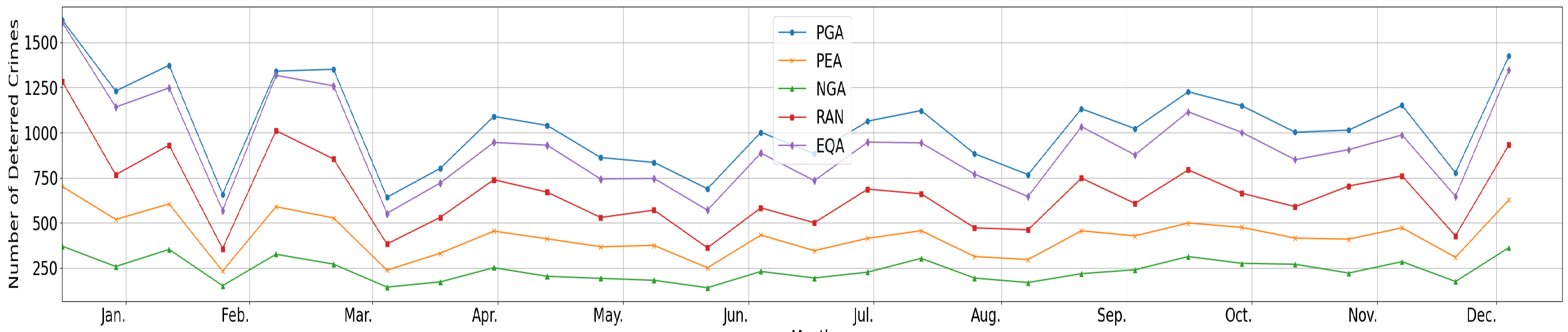
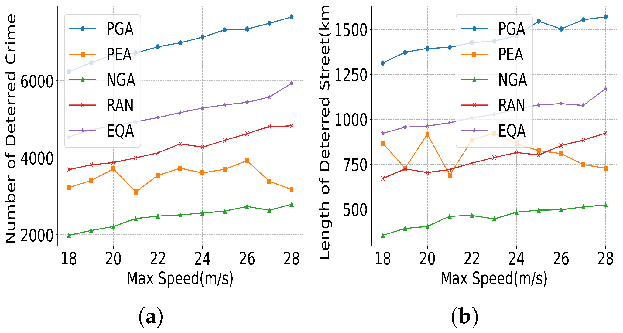
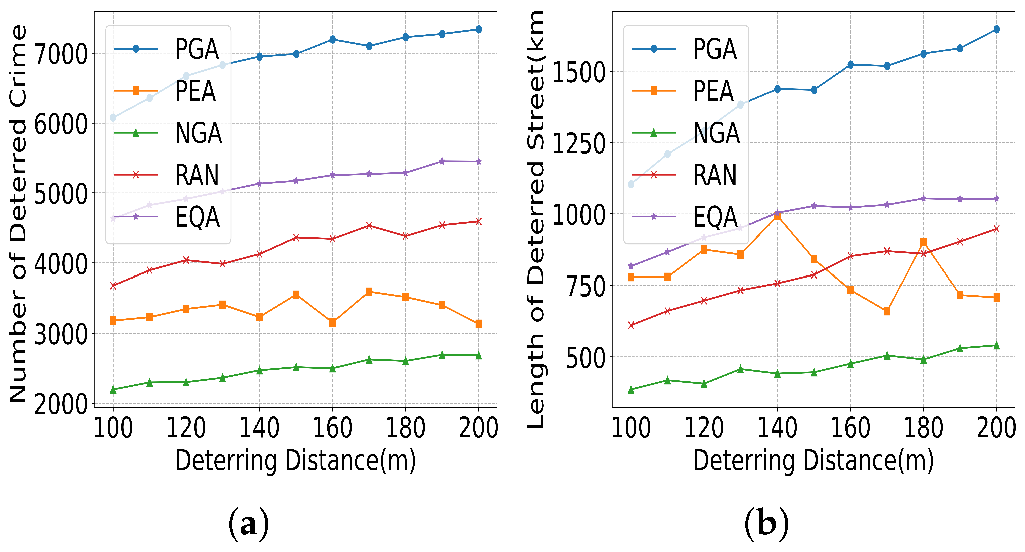
• Prediction-enhanced greedy algorithm (PGA): This method calculates the predictive crime risk and selects the maximum crime risk street for the UAV’s path.
• Prediction-enhanced EL-based algorithm (PEA): Calculate the predictive crime risk and select the predictive crime risk as a fitness function.
• Non-prediction greedy algorithm (NGA): Using historical crime statistics for crime risk and selecting the maximum non-predictive crime risk street for UAV path.
• Random (RAN): Randomly selecting locations of stations within the city area, and assign UAVs to stations with maximum coverage capacity.
• Equal assignment (EQA): Determine station location with maximum coverage capacity, and equally assign UAVs to stations.

Performance metrics: We use two metrics to assess the performance of different methods: 1. Number of Deterred Crimes (NDC): The number of crimes in 2021 at the street level covered by UAVs or stations. 2. Length of Deterred Street (LDS): The total length of streets in the scheduled UAV patrol path.

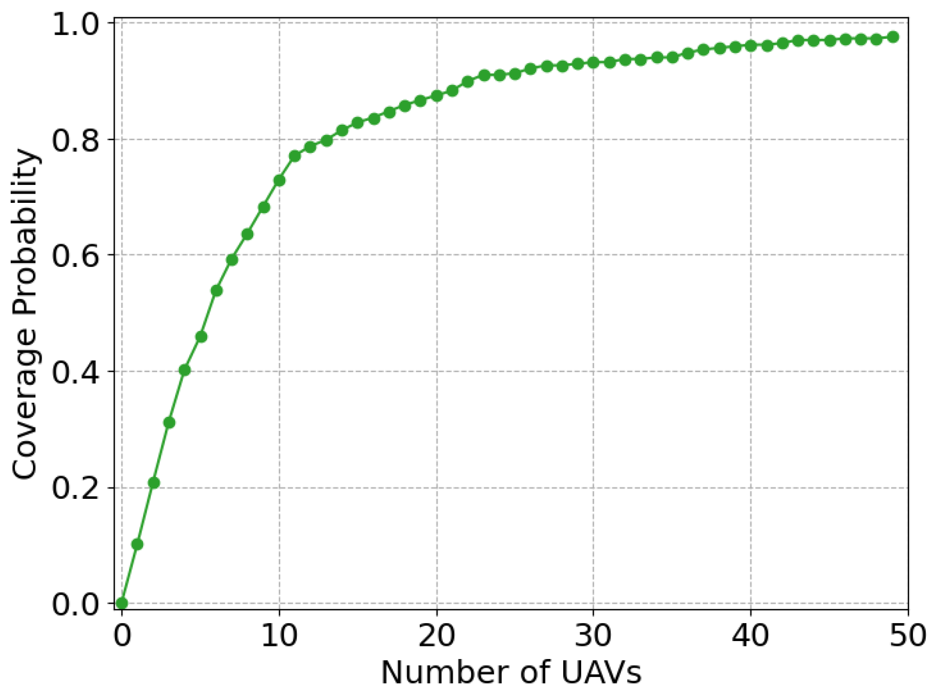
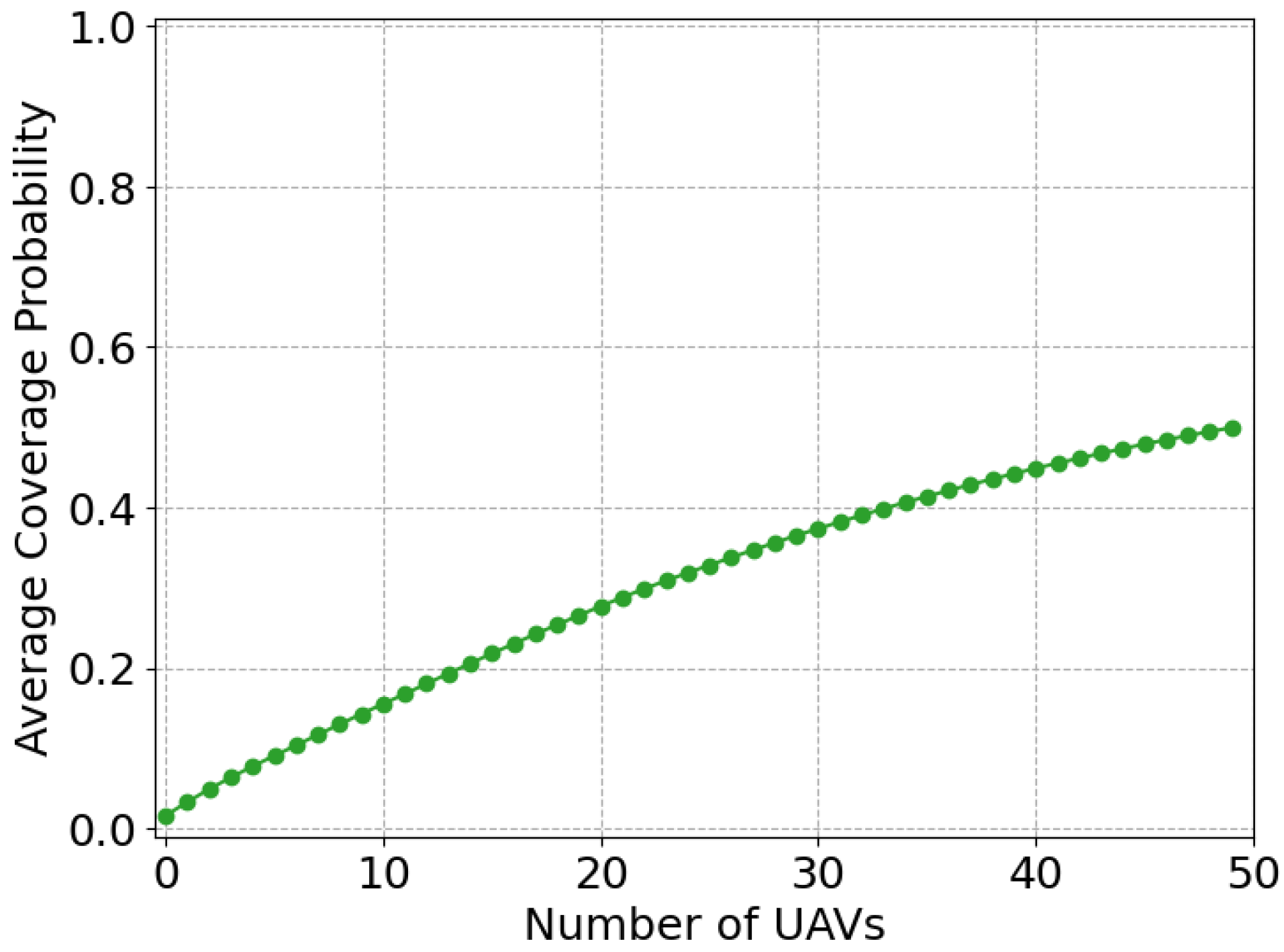
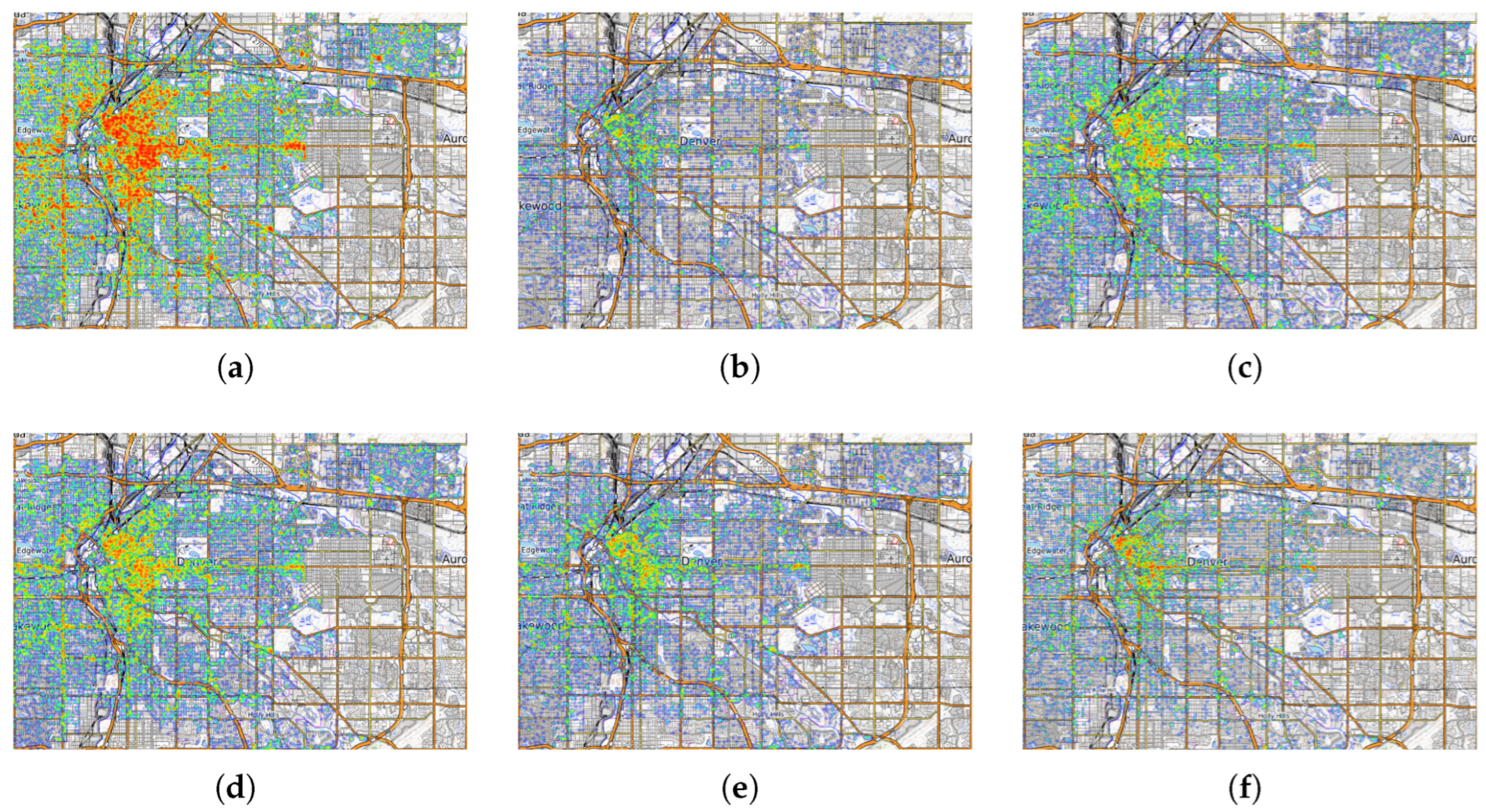
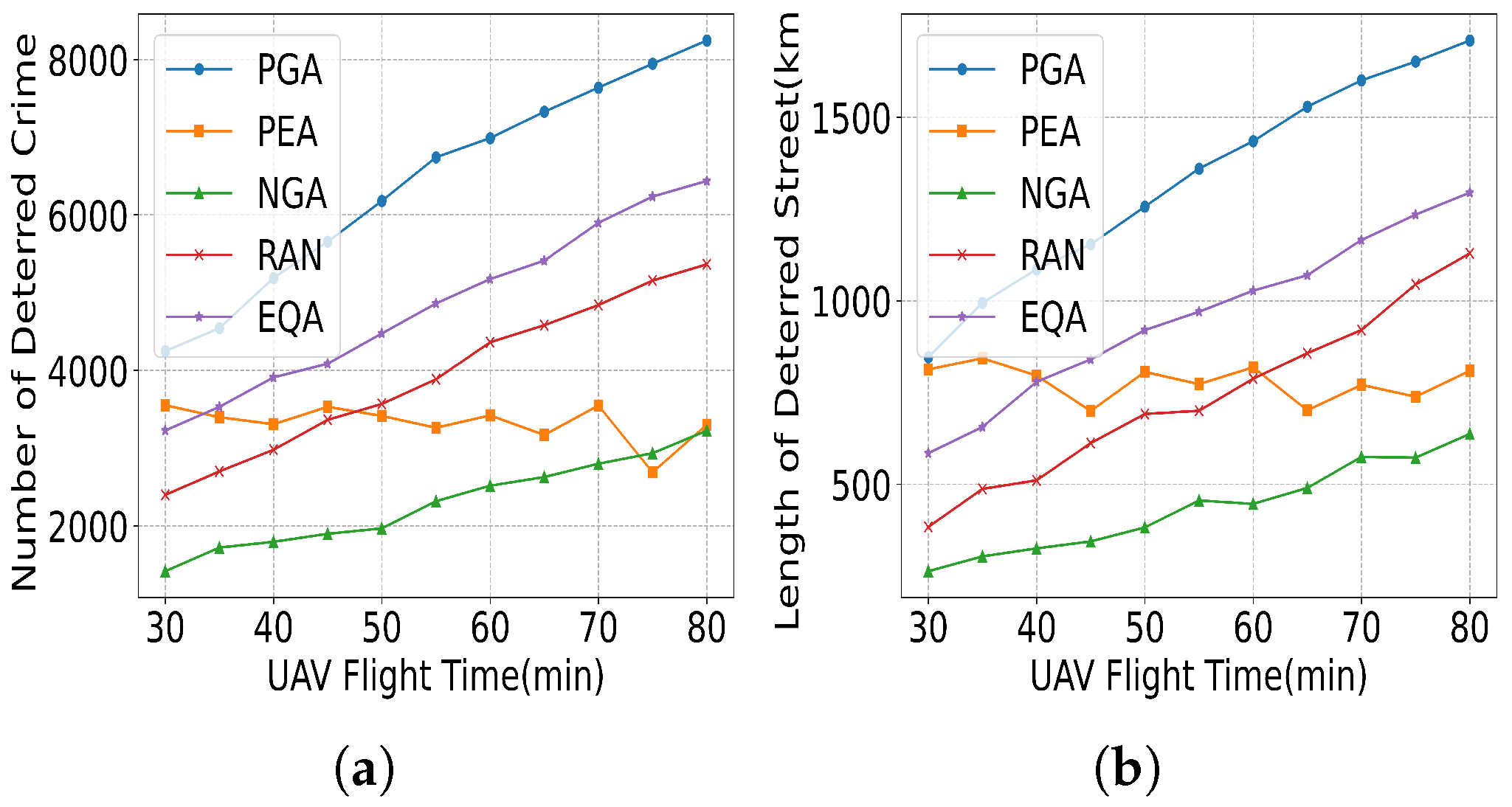
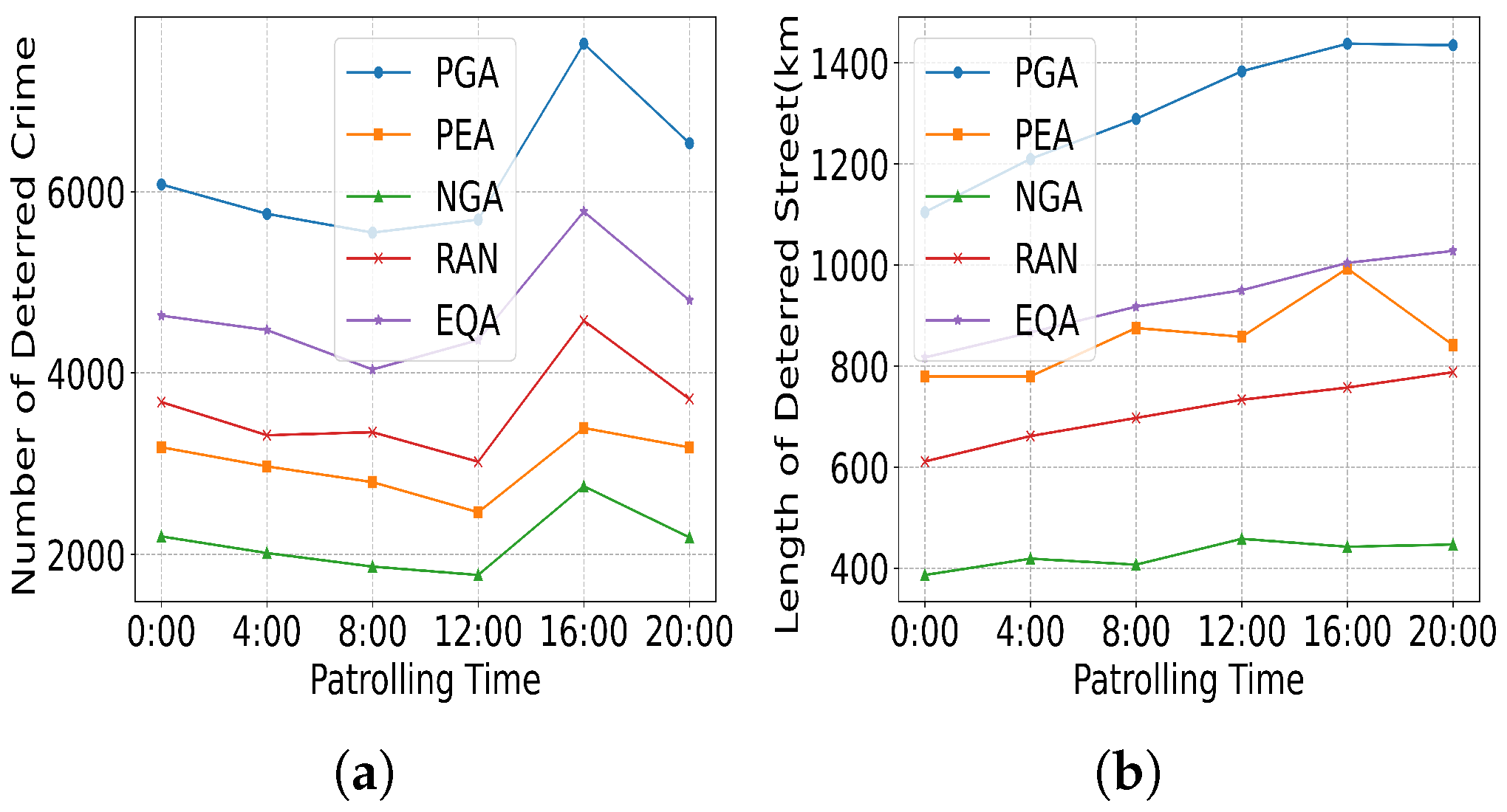
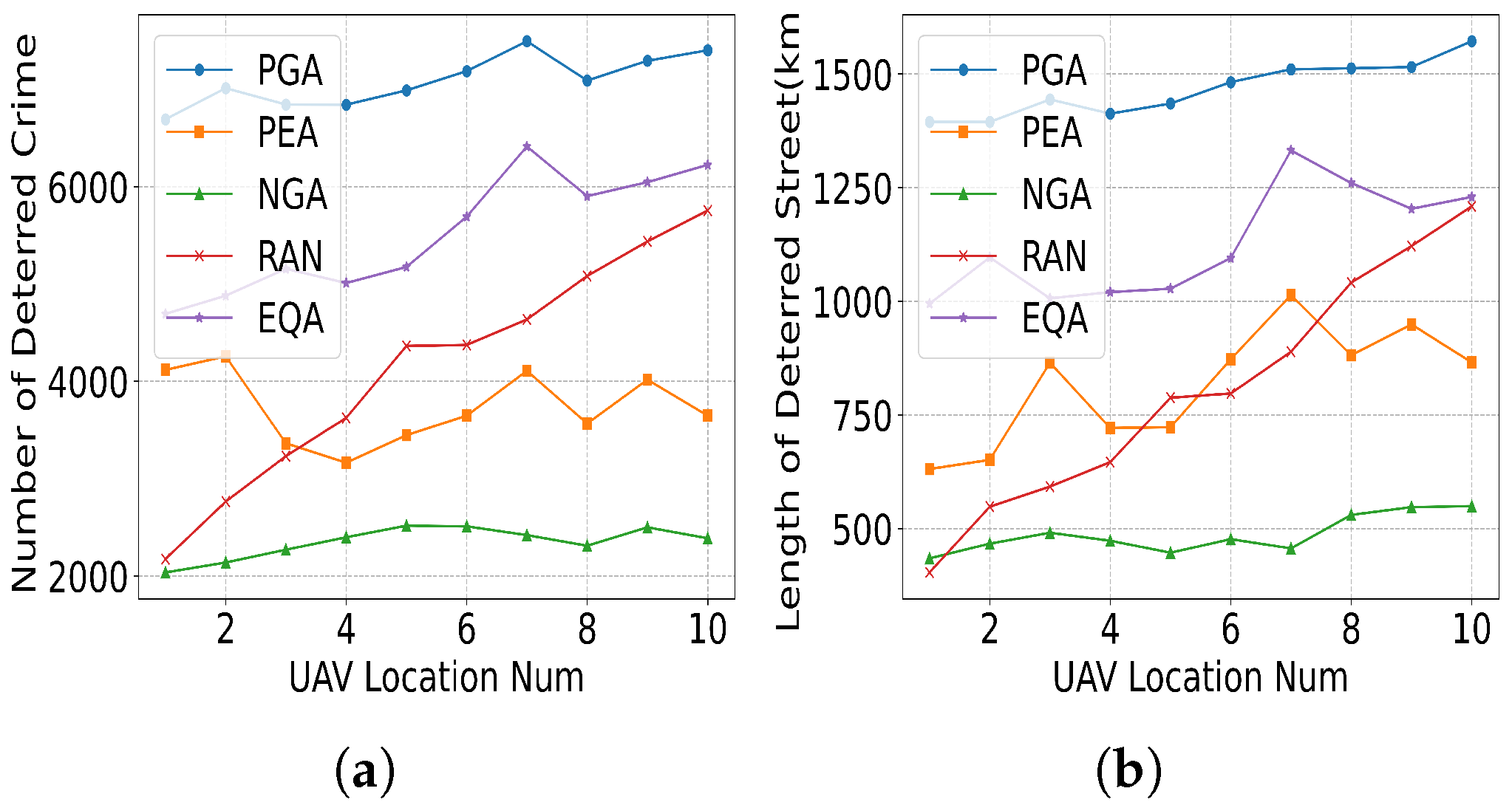
6.2. Experimental Results

To visualize the performance of our data-driven patrol framework, we present the offline-generated coverage route of a single UAV under default parameters in Figure 14. The visualization in Figure 14 incorporates multiple components: the heatmap reflects historical crime probability gradients based on five-year police data; red markers signify the UAV’s initial location; red line segments delineate patrol trajectories along high-risk streets; and blue line segments represent high-speed transit paths between these patrol areas. As shown in Figure 1, the UAV’s offline-generated flight path (default parameters) balances path cost minimization with crime risk coverage. The trajectory demonstrates the algorithm’s ability to achieve street coverage optimization through historical crime hotspot prioritization and path length minimization. While the current implementation focuses on proactive patrol patterns rather than dynamic replanning, the generated routes inherently embed adaptive features through crime probability gradients.

To validate the model generalization across different cities, we supplemented the crime dataset from Seattle [54] and Los Angeles [55]. The experimental results (Figure 15 and Figure 16) reveal distinct performance patterns across five methods (PGA, PEA, NGA, RAN, EQA) in three cities. In Figure 15, PGA outperforms others by significant margins: Denver (6264 vs. EQA’s 5892), Seattle (7101 vs. EQA’s 6505), and Los Angeles (8550 vs. EQA’s 7943). NGA consistently underperforms, with the lowest values in all cities (Denver: 2359; Seattle: 2804; Los Angeles: 3122). In Figure 16, PGA achieves the highest coverage in Los Angeles (142 km) and Denver (118 km). Notably, RAN exhibits moderate performance but lags behind PGA by 18–25% across cities. These results underscore PGA’s dominance in absolute efficacy and NGA/RAN’s limitations in both metrics.

Through comparative experiments across three cities, we found the performance patterns to be highly consistent. Therefore, we opted to use the Denver dataset as the default dataset for subsequent experiments to streamline analysis. This strategy ensures the generality of results while avoiding redundant cross-city comparisons.

Based on the default parameters and default dataset, we conduct an ablative study on each component of the framework, including the following: (1) non-prediction greedy algorithm (NGA) uses historical crime statistics instead of predictive crime risk estimation, thus omitting the crime prediction component (Section 4.1); (2) random assignment (RAN) randomly selects station locations without data-driven optimization, excluding the station placement component (Section 5.2); (3) equal assignment (EQA) allocates UAVs equally among stations without considering dynamic crime risk or station coverage, omitting optimized UAV component (Section 5.2).

The results are summarized in

Table 5. Result of ablation study.

	Metrics	Number of Deterred	Length of Deterred
Ablation		Crimes	Street (km)
PGA		6264	118
NGA (Section 4.1)		2359	38
RAN (Section 5.2)		4293	65
EQA (Section 5.2)		5892	101

, which shows a significant performance degradation when moving from PGA to NGA, where the number of deterred crimes drops from 6264 to 2359, and the length of deterred streets decreases from 118 km to 38 km. This highlights the critical role of the crime prediction module. By leveraging real-time and spatiotemporal features such as weather conditions and points of interest (POIs), the prediction model enables proactive patrolling of high-risk areas, significantly enhancing deterrence effectiveness. When comparing PGA with RAN, it becomes evident that data-driven station placement contributes substantially to overall performance. Specifically, PGA achieves a 46% increase in the number of deterred crimes and an 82% improvement in the length of deterred streets compared to RAN. This demonstrates that strategic station deployment based on historical patrol coverage significantly enhances operational efficiency. Furthermore, the comparison between PGA and EQA reveals that intelligent UAV allocation outperforms equal distribution. Although EQA achieves relatively good performance with 5892 deterred crimes and 101 km of deterred streets, PGA still improves upon these results by 6.3%, indicating that adaptive UAV allocation based on crime risk and station coverage further optimizes resource utilization. In conclusion, these findings confirm that all three components—crime prediction, station placement, and UAV allocation—are essential to achieving the superior performance of PGA.

Figure 17 illustrates the spatial distribution of crimes using heatmap. The red areas on the heatmap represent the distribution of crimes after applying different methods(the deterred crimes are removed from the heatmap). Figure 17a represents the original heatmap, showing the initial distribution of crime without any processing in Denver city. The subsequent five figures (Figure 17b–f) display the heatmaps after applying different algorithms. The changes in the heatmaps after each algorithm application reflect the algorithm’s effectiveness. These heatmaps allow us to visually assess the impact of each algorithm and compare their performance in optimizing the data. The PGA method obviously performed the best among all methods. Figure 18 shows the temporal distribution of crimes, which presents the number of deterred crimes on 30 days in 2021 by five methods. All methods exhibit synchronized fluctuation patterns, showing coincident peaks and troughs at identical temporal locations (e.g., notable spikes on Days 1 January and 18 December). Notably, the PGA method maintains superior performance across all observed time points, outperforming the second-best baseline by 8.7% on average.

(1) UAV Max Speed: Figure 19 illustrates the relationship between UAV maximum speed and crime-deterring efficacy across two metrics: number of deterred crimes (NDCs) and length of deterred streets (LDSs). As UAV speed increases from 18 m/s to 28 m/s, the PGA shows a consistent upward trend, achieving the highest performance with 7685 NDC and 1572 km LDS at 28 m/s. In contrast, the PEA exhibits significant fluctuations due to its reliance on stochastic operators, while NGA lags behind, performing 58% lower than PGA in NDC and 40% lower in LDS at 28 m/s. Baseline methods such as RAN and EQA perform poorly by 33% and 22%, respectively, highlighting the necessity of strategic resource optimization. Beyond 24 m/s, all methods experience diminishing returns, with marginal gains in NDC dropping from 22.4% (18–24 m/s) to 6.8% (24–28 m/s), suggesting that capsizing UAV speeds at 24 m/s balances efficacy and operational costs.

(2) UAV Deterring Distance: Figure 20 illustrates the effect of the UAV deterring distance on the increase in NDC and LDS under different methods. In Figure 20a, as the deterring distance increases from 100 m to 180 m, the performance of all methods improves. This is because a longer deterring distance allows the UAV to patrol more streets, potentially deterring more crimes. A similar pattern emerges in Figure 20b. The PGA achieves the highest LDS at 1500 km under the condition of 180 m deterring distance, demonstrating its capacity to strategically extend patrol coverage while maintaining efficiency. Conversely, PEA and NGA show negligible improvements in LDS, with performance plateauing early (around 500–750 km). Baseline methods such as RAN (random base station placement) and EQA (equal UAV allocation) exhibit moderate gains but remain significantly inferior to PGA, further validating the necessity of station selection and coordinated UAV allocation.

(3) UAV Flight Time: Figure 21 illustrates the effect of UAV flight time on the number of deterred crimes and the length of deterred streets under different methods. In Figure 21a, as the UAV flight time increases from 30 min to 80 min, the performance of all methods shows an upward trend. This is logical because a longer flight time allows the UAV to cover more area, potentially deterring more crimes. A similar pattern is observed in Figure 21b. The PGA method achieves the highest length of deterred streets, reaching 1500 km at 80 min, showcasing its strategic advantage in extending patrol coverage efficiently. PEA and EQA show notable increases, with PEA reaching around 1000 km and EQA around 1250 km. NGA shows the least improvement, with the length of deterred streets only increasing to about 500 km. RAN shows moderate gains, reaching around 1000 km, but remains significantly behind PGA, further emphasizing the necessity of coordinated UAV allocation and optimal station placement.

(4) UAV patrol Time: Figure 22 illustrates the impact of the patrol time on the NDC and LDS under different methods. Figure 22a exhibits significant temporal variation across all methods, with a pronounced peak at 16:00 (2000 crimes deterred by PGA) and a trough at 4:00. This trend aligns with known urban crime dynamics. In contrast, Figure 22b shows that the LDS remains relatively stable (±10% variation) across all time periods, regardless of method. This suggests that street-level crimes do not concentrate in specific corridors but exhibit dispersed patterns, limiting the impact of temporal patrol adjustments on spatial coverage.

(5) UAV numbers: Figure 23 illustrates the effect of the UAV number on the increase in the NDC and LDS under different methods. In Figure 23a, as UAV numbers increase from 5 to 50, the PGA achieves the highest NDC (12,500 crimes deterred at 50 UAVs). The near-linear growth highlights PGA’s robustness in leveraging additional UAVs to amplify deterring. In contrast, baseline methods like RAN and EQA show moderate gains but plateau earlier (at 30–40 UAVs), constrained by inefficient spatial distribution strategies. Similar trends can be observed in Figure 23b, with PGA maximizing LDS (50 km at 50 UAVs). The diminishing returns beyond 45 UAVs suggest deploying 40–45 units for cost–efficacy balance.

(6) UAV Station Number: Figure 24 illustrates the impact of UAV station numbers on the increase in the NDC and LDS under different algorithms. In Figure 24a, as the number of UAV stations increases from 1 to 10, the PGA achieves only a marginal NDC improvement (6671 to 7100 crimes deterred), despite its reliance on high-coverage-capacity station placement. In contrast, the RAN method shows erratic performance (+176.19%), as stochastic station placement fails to consistently target high-risk areas. Figure 24b follows a similar pattern. PGA achieves peak LDS (1500 km) at 6 stations, after which further additions yield diminishing returns (only 4% improvement from 6 to 10 stations). It suggests that the number of UAV stations has a limited impact on crime deterring beyond an optimal threshold (4–6 stations).

Experimental result shows that the PGA method demonstrates significant advantages in multi-parameter optimization. By integrating crime prediction, maximum coverage capacity station placement, and dynamic UAV allocation, PGA improves the number of deterred crimes (NDCs) by 45% to 58% and the length of deterred streets (LDSs) by 33% to 60% in scenarios such as maximum speed of UAV (24 m/s as the efficiency threshold), deterring distance (180 m), flight time (80 min), and peak-hour patrols (16:00), compared to baseline methods (PEA, NGA, RAN, EQA). Our findings include the following: (1) algorithm performance is constrained by physical limitations and strategic bottlenecks, with diminishing returns when speed exceeds 24 m/s or the number of UAVs exceeds 45, and (2) the number of stations has a limited impact on performance, with 4–6 high-coverage stations achieving 90% of peak efficiency. The research concludes by advocating for the PGA as the core framework, prioritizing optimization of prediction models and UAV allocation over the simple increase in UAV scale, and providing an efficient and scalable UAV deployment paradigm for urban security.

7. Conclusions

In this paper, we propose a data-driven framework for scheduling patrol UAVs to deter street crimes, which includes a data processing module, an online patrol path planning module, and an offline UAV station siting module. The framework utilizes a prediction-enhanced method to estimate street-level crime risk to guide UAVs to patrol high-risk streets more efficiently. The offline module conducts a data-driven estimation of the deterring effect of candidate UAV stations and optimizes their locations, along with determining the appropriate number of UAVs for each station. Using a 6-year crime dataset and the corresponding contextual datasets, the proposed framework is comprehensively evaluated. The evaluation shows that, compared with baselines, the proposed framework improves the deterring performance by $58.49\%$ on average, and up to $157.32\%$ in extreme cases.

References

1. Statista. Deaths by Homicide per 100,000 Resident Population in the U.S. from 1950 to 2019. Published by Statista. 2021. Available online: https://www.statista.com/statistics/187592/death-rate-from-homicide-in-the-us-since-1950/ (accessed on 11 May 2021).
2. Miller, T.R.; Cohen, M.A.; Swedler, D.I.; Ali, B.; Hendrie, D.V. Incidence and costs of personal and property crimes in the USA, 2017. J. Benefit-Cost Anal. 2021, 12, 24–54. [Google Scholar] [CrossRef]
3. Caplan, J.M.; Kennedy, L.W.; Petrossian, G. Police-monitored CCTV cameras in Newark, NJ: A quasi-experimental test of crime deterrence. J. Exp. Criminol. 2011, 7, 255–274. [Google Scholar] [CrossRef]
4. Hochstetler, J.; Hochstetler, L.; Fu, S. An optimal police patrol planning strategy for smart city safety. In Proceedings of the 2016 IEEE 18th International Conference on High Performance Computing and Communications; IEEE 14th International Conference on Smart City; IEEE 2nd International Conference on Data Science and Systems (HPCC/SmartCity/DSS), Sydney, NSW, Australia, 12–14 December 2016; pp. 1256–1263. [Google Scholar]
5. Weisburd, S. Police presence, rapid response rates, and crime prevention. Rev. Econ. Stat. 2021, 103, 280–293. [Google Scholar] [CrossRef]
6. Nagin, D.S.; Solow, R.M.; Lum, C. Deterrence, criminal opportunities, and police. Criminology 2015, 53, 74–100. [Google Scholar] [CrossRef]
7. Adams, I.T.; Mourtgos, S.; Nix, J. Turnover in Large US Police Agencies Following the George Floyd Protests. J. Crim. Justice 2023, 88, 102105. [Google Scholar] [CrossRef]
8. Voice of Europe Netherlands: Police Staff Shortages Persist, Projected to Continue Until 2027. 2023. Available online: https://www.voiceofeurope.com/netherlands-police-staff-shortages-persist-projected-to-continue-2027/ (accessed on 30 November 2023).
9. Statistics Canada. Decrease in the Rate of Police Strength in Canada in 2022. Published by The Daily, Statistics Canada. 2022. Available online: https://www150.statcan.gc.ca/n1/daily-quotidien/230327/dq230327a-eng.htm (accessed on 11 May 2025).
10. Ryan-Mosley, T. A New Map of NYC’s Cameras Shows More Surveillance in Black and Brown Neighborhoods. Published by MIT Technology Review. 2022. Available online: https://www.technologyreview.com/2022/02/14/1045333/map-nyc-cameras-surveillance-bias-facial-recognition/ (accessed on 11 May 2025).
11. Welsh, B.C.; Farrington, D.P. Public area CCTV and crime prevention: An updated systematic review and meta-analysis. Justice Q. 2009, 26, 716–745. [Google Scholar] [CrossRef]
12. Phillips, C. A review of CCTV evaluations: Crime reduction effects and attitudes towards its use. Crime Prev. Stud. 1999, 10, 123–155. [Google Scholar]
13. Johnson, K. This New Autonomous Drone for Cops Can Track You in the Dark. Published by Wired. 2023. Available online: https://www.wired.com/story/new-autonomous-drone-for-cops-can-track-you-in-the-dark/ (accessed on 11 May 2025).
14. Criminal Legal News. Armed Police Drones Are Coming. Published by Criminal Legal News. 2022. Available online: https://www.criminallegalnews.org/news/2022/feb/15/armed-police-drones-are-coming/ (accessed on 11 May 2023).
15. Huang, H.; Savkin, A.V.; Ni, W. Online UAV trajectory planning for covert video surveillance of mobile targets. IEEE Trans. Autom. Sci. Eng. 2021, 19, 735–746. [Google Scholar] [CrossRef]
16. Zengin, U.; Dogan, A. Real-time target tracking for autonomous UAVs in adversarial environments: A gradient search algorithm. IEEE Trans. Robot. 2007, 23, 294–307. [Google Scholar] [CrossRef]
17. Zheng, Y.J.; Du, Y.C.; Ling, H.F.; Sheng, W.G.; Chen, S.Y. Evolutionary collaborative human-UAV search for escaped criminals. IEEE Trans. Evol. Comput. 2019, 24, 217–231. [Google Scholar] [CrossRef]
18. Gao, J.; Wang, Q.; Li, Z.; Zhang, X.; Hu, Y.; Han, Q.; Pan, Y. Towards Efficient Urban Emergency Response Using UAVs Riding Crowdsourced Buses. IEEE Internet Things J. 2024, 11, 22439–22455. [Google Scholar] [CrossRef]
19. Zhang, H.; Vorobeychik, Y. Submodular optimization with routing constraints. In Proceedings of the AAAI Conference on Artificial Intelligence, Phoenix, AZ, USA, 12–17 February 2016; Volume 30. [Google Scholar]
20. Bian, C.; Feng, C.; Qian, C.; Yu, Y. An efficient evolutionary algorithm for subset selection with general cost constraints. In Proceedings of the AAAI Conference on Artificial Intelligence, New York, NY, USA, 7–12 February 2020; Volume 34, pp. 3267–3274. [Google Scholar]
21. Bozcan, I.; Kayacan, E. AU-AIR: A Multi-modal Unmanned Aerial Vehicle Dataset for Low Altitude Traffic Surveillance. In Proceedings of the 2020 IEEE International Conference on Robotics and Automation (ICRA), Paris, France, 31 May–31 August 2020; pp. 8504–8510. [Google Scholar] [CrossRef]
22. Trotta, A.; Andreagiovanni, F.D.; Di Felice, M.; Natalizio, E.; Chowdhury, K.R. When UAVs ride a bus: Towards energy-efficient city-scale video surveillance. In Proceedings of the IEEE INFOCOM 2018—IEEE Conference on Computer Communications, Honolulu, HI, USA, 16–19 April 2018; pp. 1043–1051. [Google Scholar]
23. Li, B.; Fu, C.; Ding, F.; Ye, J.; Lin, F. ADTrack: Target-Aware Dual Filter Learning for Real-Time Anti-Dark UAV Tracking. In Proceedings of the 2021 IEEE International Conference on Robotics and Automation (ICRA), Xian, China, 30 May–5 June 2021; pp. 496–502. [Google Scholar] [CrossRef]
24. Savkin, A.V.; Huang, H. Navigation of a UAV network for optimal surveillance of a group of ground targets moving along a road. IEEE Trans. Intell. Transp. Syst. 2021, 23, 9281–9285. [Google Scholar] [CrossRef]
25. Vanegas, F.; Campbell, D.; Eich, M.; Gonzalez, F. UAV based target finding and tracking in GPS-denied and cluttered environments. In Proceedings of the 2016 IEEE/RSJ International Conference on Intelligent Robots and Systems (IROS), Daejeon, Republic of Korea, 9–14 October 2016; pp. 2307–2313. [Google Scholar]
26. Pan, Y.; Li, S.; Chen, Q.; Zhang, N.; Cheng, T.; Li, Z.; Guo, B.; Han, Q.; Zhu, T. Efficient schedule of energy-constrained UAV using crowdsourced buses in last-mile parcel delivery. In Proceedings of the ACM on Interactive, Mobile, Wearable and Ubiquitous Technologies; Association for Computing Machinery: New York, NY, USA, 2021; Volume 5, pp. 1–23. [Google Scholar]
27. Xiang, C.; Zhou, Y.; Dai, H.; Qu, Y.; He, S.; Chen, C.; Yang, P. Reusing delivery drones for urban crowdsensing. IEEE Trans. Mob. Comput. 2021, 22, 2972–2988. [Google Scholar] [CrossRef]
28. Beg, A.; Qureshi, A.R.; Sheltami, T.; Yasar, A. UAV-enabled intelligent traffic policing and emergency response handling system for the smart city. Pers. Ubiquitous Comput. 2021, 25, 33–50. [Google Scholar] [CrossRef]
29. Liu, Y.V.; Kang, W.; Maskály, J.; Ivković, S.K. Policing from the Sky: A Case Study of the Police Use of Drones in South Korea. In Exploring Contemporary Police Challenges; Routledge: London, UK, 2022; pp. 167–180. [Google Scholar]
30. Nader, E.; Wasileski, G.; Poteyeva, M. Community Perceptions, Concerns for Privacy, and Support for Law Enforcement Use of Aerial Surveillance in Baltimore. Crime Delinq. 2023, 71, 00111287231189720. [Google Scholar] [CrossRef]
31. Saulnier, A.; Thompson, S.N. Police UAV use: Institutional realities and public perceptions. Polic. Int. J. Police Strateg. Manag. 2016, 39, 680–693. [Google Scholar] [CrossRef]
32. Ratcliffe, J.H.; Taniguchi, T.; Groff, E.R.; Wood, J.D. The Philadelphia foot patrol experiment: A randomized controlled trial of police patrol effectiveness in violent crime hotspots. Criminology 2011, 49, 795–831. [Google Scholar] [CrossRef]
33. Koper, C.S. Just enough police presence: Reducing crime and disorderly behavior by optimizing patrol time in crime hot spots. Justice Q. 1995, 12, 649–672. [Google Scholar] [CrossRef]
34. Koper, C.S.; Mayo-Wilson, E. Police strategies to reduce illegal possession and carrying of firearms: Effects on gun crime. Campbell Syst. Rev. 2012, 8, 1–53. [Google Scholar] [CrossRef]
35. Blanes i Vidal, J.; Kirchmaier, T. The effect of police response time on crime clearance rates. Rev. Econ. Stud. 2018, 85, 855–891. [Google Scholar] [CrossRef]
36. Ratcliffe, J.H.; Taniguchi, T.; Taylor, R.B. The crime reduction effects of public CCTV cameras: A multi-method spatial approach. Justice Q. 2009, 26, 746–770. [Google Scholar] [CrossRef]
37. Brayne, S.; Christin, A. Technologies of crime prediction: The reception of algorithms in policing and criminal courts. Soc. Probl. 2021, 68, 608–624. [Google Scholar] [CrossRef] [PubMed]
38. Wang, H.; Kifer, D.; Graif, C.; Li, Z. Crime rate inference with big data. In Proceedings of the 22nd ACM SIGKDD International Conference on Knowledge Discovery and Data Mining, San Francisco, CA, USA, 13–17 August 2016; pp. 635–644. [Google Scholar]
39. Yi, F.; Yu, Z.; Zhuang, F.; Guo, B. Neural Network based Continuous Conditional Random Field for Fine-grained Crime Prediction. In Proceedings of the International Joint Conference on Artificial Intelligence, Macao, China, 10–16 August 2019; pp. 4157–4163. [Google Scholar]
40. Huang, C.; Zhang, J.; Zheng, Y.; Chawla, N.V. DeepCrime: Attentive hierarchical recurrent networks for crime prediction. In Proceedings of the 27th ACM international Conference on Information and Knowledge Management, Turin, Italy, 22–26 October 2018; pp. 1423–1432. [Google Scholar]
41. Zhao, X.; Tang, J. Modeling Temporal-Spatial Correlations for Crime Prediction. In Proceedings of the 2017 ACM on Conference on Information and Knowledge Management, New York, NY, USA, 6–10 November 2017; CIKM ’17. pp. 497–506. [Google Scholar] [CrossRef]
42. Zhao, X.; Fan, W.; Liu, H.; Tang, J. Multi-type urban crime prediction. In Proceedings of the AAAI Conference on Artificial Intelligence, Vancouver, BC, Canada, 28 February–1 March 2022; Volume 36, pp. 4388–4396. [Google Scholar]
43. Zhang, X.; Liu, L.; Lan, M.; Song, G.; Xiao, L.; Chen, J. Interpretable machine learning models for crime prediction. Comput. Environ. Urban Syst. 2022, 94, 101789. [Google Scholar] [CrossRef]
44. Mooney, P. Denver Crime Data. 2014. Available online: https://www.kaggle.com/datasets/paultimothymooney/denver-crime-data (accessed on 1 October 2024).
45. Open Street Map. OpenStreetMap. 2024. Available online: https://www.openstreetmap.org/ (accessed on 14 June 2024).
46. Raspisaniye Pogodi Ltd. Weather Forecast and Observational Data for Denver. Published by Raspisaniye Pogodi Ltd. 2025. Available online: https://rp5.ru/%D0%9F%D0%BE%D0%B3%D0%BE%D0%B4%D0%B0_%D0%B2_%D0%94%D0%B5%D0%BD%D0%B2%D0%B5%D1%80%D0%B5 (accessed on 11 May 2025).
47. Evans, W.N.; Owens, E.G. COPS and Crime. J. Public Econ. 2007, 91, 181–201. [Google Scholar] [CrossRef]
48. Di Tella, R.; Schargrodsky, E. Do police reduce crime? Estimates using the allocation of police forces after a terrorist attack. Am. Econ. Rev. 2004, 94, 115–133. [Google Scholar] [CrossRef]
49. Yan, L.; Shen, H.; Zhao, J.; Xu, C.; Luo, F.; Qiu, C.; Zhang, Z.; Mahmud, S. Catcharger: Deploying in-motion wireless chargers in a metropolitan road network via categorization and clustering of vehicle traffic. IEEE Internet Things J. 2021, 9, 9525–9541. [Google Scholar] [CrossRef]
50. Corcoran, J.; Zahnow, R. Weather and crime: A systematic review of the empirical literature. Crime Sci. 2022, 11, 16. [Google Scholar] [CrossRef]
51. Rizeei, H.M.; Pradhan, B.; Saharkhiz, M.A. Allocation of emergency response centres in response to pluvial flooding-prone demand points using integrated multiple layer perceptron and maximum coverage location problem models. Int. J. Disaster Risk Reduct. 2019, 38, 101205. [Google Scholar] [CrossRef]
52. Qian, C.; Shi, J.C.; Yu, Y.; Tang, K. On Subset Selection with General Cost Constraints. In Proceedings of the International Joint Conference on Artificial Intelligence, Melbourne, Australia, 19–25 August 2017; Volume 17, pp. 2613–2619. [Google Scholar]
53. Horel, T.; Singer, Y. Maximization of approximately submodular functions. Adv. Neural Inf. Process. Syst. 2016, 29, 3053–3061. [Google Scholar]
54. Department, S.P. Seattle Police Department 911 Incident Response. 2024. Available online: https://www.kaggle.com/datasets/sohier/seattle-police-department-911-incident-response (accessed on 2 October 2024).
55. Department, L.A.P. Crime in Los Angeles. 2024. Available online: https://www.kaggle.com/datasets/cityofLA/crime-in-los-angeles (accessed on 1 October 2024).
Figure 1. Heatmap of crimes regions.
Drones 09 00449 g001
Figure 2. Distribution of high-risk streets.
Drones 09 00449 g002
Figure 3. Influence of regions on crimes.
Drones 09 00449 g003
Figure 4. Crimes in daytime.
Drones 09 00449 g004
Figure 5. CDF of time between crimes.
Drones 09 00449 g005
Figure 6. Street length and crime number.
Drones 09 00449 g006
Figure 7. Crime deterring model [5].
Drones 09 00449 g007
Figure 8. UAV patrol model.
Drones 09 00449 g008
Figure 9. Framework.
Drones 09 00449 g009
Figure 10. Prediction-enhanced street-level deterring effect estimation model.
Drones 09 00449 g010
Figure 11. Distribution of covered streets.
Drones 09 00449 g011
Figure 12. Influence of UAV # on a street.
Drones 09 00449 g012
Figure 13. Average influence of UAV #.
Drones 09 00449 g013
Figure 14. Example path for 1 UAV.
Drones 09 00449 g014
Figure 15. Number of deterred crimes.
Drones 09 00449 g015
Figure 16. Length of deterred streets.
Drones 09 00449 g016
Figure 17. Heatmap of crimes after applying different methods. (a) Original heatmap. (b) PGA. (c) PEA. (d) NGA. (e) RAN. (f) EQA.
Drones 09 00449 g017
Figure 18. Deterred crimes on different dates.
Drones 09 00449 g018
Figure 19. Influence of max speed. (a) Performance in NDC. (b) Performance in LDS.
Drones 09 00449 g019
Figure 20. Influence of deterring distance. (a) Performance in NDC. (b) Performance in LDS.
Drones 09 00449 g020
Figure 21. Influence of UAV flight time. (a) Performance in NDC. (b) Performance in LDS.
Drones 09 00449 g021
Figure 22. Influence of patrol time. (a) Performance in NDC. (b) Performance in LDS.
Drones 09 00449 g022
Figure 23. Influence of UAV number. (a) Performance in NDC. (b) Performance in LDS.
Drones 09 00449 g023
Figure 24. Influence of station number. (a) Performance in NDC. (b) Performance in LDS.
Drones 09 00449 g024