High-Precision Trajectory-Tracking Control of Quadrotor UAVs Based on an Improved Crested Porcupine Optimiser Algorithm and Preset Performance Self-Disturbance Control

Abstract

In view of the difficulties encountered when tuning parameters and the lack of anti-interference capabilities exhibited by high-precision trajectory-tracking control of quadrotor UAVs in complex dynamic environments, this paper proposes a fusion control framework based on an improved crowned pig optimisation algorithm (ICPO) and preset performance anti-disturbance control (PPC-ADRC). Initially, this paper addresses the limited convergence efficiency of the traditional crowned pig algorithm (CPO) by introducing a dynamic time threshold mechanism and an adaptability-based directed elimination strategy to balance the algorithm’s global exploration and local development capabilities. This results in a significant improvement in the convergence speed and optimisation accuracy. Secondly, a hierarchical control architecture is designed, with the outer loop using a PPC-ADRC controller to dynamically constrain the tracking error boundary using an exponential performance funnel function and a combined state observer (ESO) to estimate the compound disturbance in real time. The inner-loop attitude control uses ADRC, and the 24-dimensional parameters of the ADRC (including the ESO bandwidth and non-linear feedback gain) are optimised autonomously using the ICPO to achieve efficient parameter tuning. The simulation experiments demonstrate that, in comparison with the original CPO, the ICPO attains an average fitness ranking that is superior in the CEC2014–2022 benchmark test, thereby substantiating its global optimisation capability. In the PPC-ADRC controller parameter optimisation, the preset performance of the ICPO-tuned PPC-ADRC controller (PPC-ADRC) is superior to that of the particle swarm optimisation (PSO), genetic algorithm (GA) and original CPO. The ICPO-based PPC-ADRC controller is shown to reduce the total error by more than 45.6% compared to the ordinary ADRC controller in the task of tracking a spiral trajectory, and it effectively reduces the overshoot. Its capacity to withstand complex wind disturbances is notably superior to that of the traditional PID and ADRC architectures. Stability analysis further proves that the system satisfies the Lyapunov convergence condition in a finite time. This research provides a theoretical foundation for the high-precision control of UAVs in complex dynamic environments.

1. Introduction

Quadrotor UAVs have been shown to offer significant advantages in complex environment inspection [1], autonomous logistics [2] and disaster relief [3] due to their high mobility and flexible deployment capabilities. Nevertheless, their underactuated characteristics, strong non-linear dynamic models and susceptibility to external disturbances render high-precision trajectory tracking and robust control challenging. Although traditional PID control [4] has a simple structure, it has limitations, such as large steady-state errors and empirical parameter tuning difficulty in dynamic environments [5,6]. Adaptive disturbance rejection control (ADRC) is a methodology that estimates and compensates for disturbances in real time using an extended state observer (ESO), thereby significantly improving the system’s anti-interference ability. However, its multi-parameter coupling characteristics result in inefficient tuning [7], thus limiting its practical engineering applications.

In recent years, the combination of intelligent optimisation algorithms and the self-tuning of controller parameters has become a research hotspot. Particle swarm optimisation (PSO) and genetic algorithms (GAs) are widely used to improve controller performance and tune controller parameters. However, traditional algorithms are prone to local optima in high-dimensional parameter spaces and have insufficient search efficiency. For example, an adaptive disturbance rejection controller (ADRC) based on improved particle swarm algorithm optimisation was proposed. By introducing an adaptive adjustment mechanism for the inertia weight, the problem of ADRC parameter tuning being dependent on experience is solved and the practical performance of the controller is improved [8]. In view of the problem of excessive ADRC parameters and difficulty in tuning in the attitude control of quadrotor aircraft, a particle swarm optimisation algorithm with variable weights and hybridisation has been proposed. By dynamically adjusting the inertia weights and introducing hybrid evolution, it avoids falling into local optima. The optimised controller shows good control effects in the attitude control of quadrotor aircraft [9]. In order to address the difficulty of ADRC parameter tuning, a modified genetic algorithm was proposed. By establishing a target evaluation function for the control effect of the controller and comprehensively considering the dynamic performance and input constraints, the optimised ADRC controller performed well in terms of its anti-interference ability and fast response [10]. In addition, a four-rotor ADRC controller parameter optimisation method based on an improved artificial bee colony algorithm has also been proposed. Through adaptive exploration and development strategies, the global search ability and convergence speed of the algorithm have been improved [11]. In the control of permanent magnet synchronous motors, a study combined the particle swarm optimisation algorithm with an improved FAL function for ADRC parameter tuning, which significantly reduced the overshoot and shortened the regulation time [12].

In addition, the optimal design of a self-immune controller based on an improved ant colony search algorithm (BAS) has also received widespread attention. The study proposed an improved ant colony search algorithm that solves the problem of premature convergence that is prone to occur in the later stages of the traditional BAS algorithm by introducing a quantum evolution strategy. The improved algorithm is used to optimise the parameters of the self-immune controller (ADRC), which significantly improves the control accuracy and response speed and is suitable for complex engineering problems [13]. At the same time, an artificial fish swarm algorithm (AFSA)-based self-resonant controller optimisation method was proposed. A hybrid algorithm composed of the AFSA and particle swarm optimisation (PSO) was used to optimise the ADRC parameters. By combining the advantages of the two, the method showed good control performance in UAV attitude control [14] and verified the effectiveness of the optimisation design for ADRC in complex systems.

However, the majority of extant methods utilise conventional intelligent optimisation algorithms, with particle swarm optimisation and genetic algorithms being notable examples. However, these methods continue to encounter challenges, such as the constrained convergence speed and vulnerability to local optima, in achieving a dynamic balance between global exploration and local development. They cannot adjust the parameters in the face of dynamic disturbances adaptively and regulate the computational complexity arising from the coupling of high-dimensional parameters. The beetle antennae search algorithm is a single-objective optimisation algorithm suitable for low-dimensional fast optimisation, but it has limited global search ability and is prone to local optima in high dimensions; the artificial fish swarm algorithm is a swarm algorithm suitable for complex multi-objective problems. However, the high computational cost of the swarm coordination mechanism limits its application in real-time control systems.

In light of these limitations, this study proposes the crown-crested porcupine optimisation algorithm (CPO) [15], which emulates the cooperative defence behaviour of the crown-crested porcupine to establish a dynamically balanced global exploration and local development mechanism. This approach offers a novel biomimetic solution for the optimisation of high-dimensional non-linear ADRC controller parameters.

The CPO [16] is an emerging bionic optimisation strategy that balances global exploration and local exploitation capabilities by simulating the multimodal defence behaviour of the crested porpoise, including vision, hearing, smell and physical attacks. Nevertheless, the CPO’s fixed elimination mechanism does not fully consider individual differences in fitness, resulting in limited convergence efficiency. The present paper proposes an improved CPO (ICPO) algorithm to address this problem. The exploration–exploitation ratio is dynamically adjusted by introducing a time-varying deterministic threshold (Tz), and a directed elimination strategy based on fitness [17,18] is designed to optimise the pressure distribution of the population.

Furthermore, the ICPO is deeply integrated with preset performance self-adaptive disturbance rejection control (PPC-ADRC). PPC-ADRC dynamically constrains the tracking error through the exponential performance funnel function ϖ(t) and compensates for compound disturbances in real time with the ESO. In contrast, the ICPO autonomously optimises the numerous parameters of the ADRC (including 24-dimensional parameters such as the ESO bandwidth and non-linear feedback gain), thereby circumventing the limitations of conventional methods that depend on empirical parameter adjustment.

The main innovations in this paper are as follows. First, the improved crowned pig optimisation (ICPO) algorithm is improved. Through a dynamic thresholding mechanism and an adaptive elimination strategy, it effectively balances global exploration and local development capabilities, improving the convergence speed and global optimisation efficiency. Second, a deep integration framework of the ICPO and PPC-ADRC is constructed, which uses a preset performance function to constrain the error boundary dynamically and uses the ICPO to realise self-tuning of ADRC parameters. It overcomes the limitations of traditional methods that rely on empirical parameter tuning, providing an efficient and robust solution for UAV control in complex environments. Finally, dual-platform simulation using MATLAB (https://www.mathworks.com/products/matlab.html) and RflySim further verifies the superior response performance of PPC-ADRC and the effectiveness of the ICPO parameter tuning. The above innovations enable a compelling exploration of high-precision UAV control in complex dynamic environments and the self-tuning of ADRC controller parameters with both efficiency and reliability.

The full text is structured as follows. Section 2 establishes a dynamic model of a quadrotor UAV and designs a hierarchical control architecture. Section 3 proposes an improved crown porcupine optimisation algorithm and describes its fusion mechanism with ADRC. Section 4 verifies the theoretical reliability of the control system through stability analysis. Section 5 presents the results of the simulation experiments and comparative analysis. Finally, the full text concludes and looks forward to future research directions.

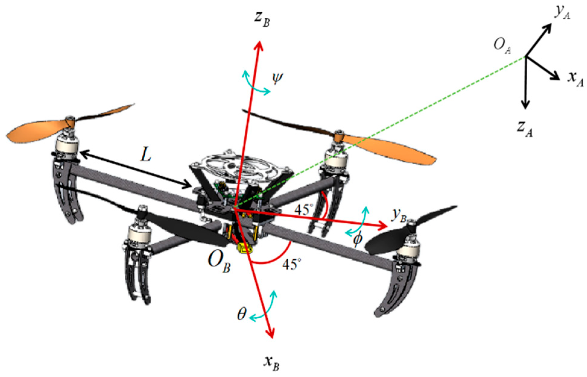
2. Modelling of Four-Rotor UAVs

2.1. Mathematical Modelling of Quadcopter UAVs

In this study, a quadrotor with a typical “X” configuration (the nose of the aircraft is marked in red and is at an angle of 45° to the plane of the frame) is selected as the research object. In order to accurately characterise the dynamic properties of the vehicle, two sets of spatial reference systems, the ground inertial coordinate system ($O_A-x_A,y_A,z_A$) and the airframe coordinate system ($O_B-x_B,y_B,z_B$), are established, as shown in Figure 1, where the Z-axis of the inertial coordinate system points to the centre of the Earth vertically. The Z-axis of the airframe coordinate system has the centre of mass of the vehicle as the origin, and the Z-axis coincides with the direction of the thrust vector.

In the process of establishing the mathematical model, the following basic assumptions are followed in this study:

(1)

the aircraft is a rigid body with complete geometric and structural symmetry;

(2)

the mass characteristics and rotational moment of inertia of the system are kept constant;

(3)

the geometrical centre of symmetry and the spatial position of the centre of mass coincide.

Based on the above assumptions, the classical Newton–Euler method is used to establish the complete dynamical equations containing the motion of six degrees of freedom in space, and the mathematical model characterising the spatial motion of the quadrotor is finally derived, as shown in Equation (1).

$$\left[\begin{array}{c}\ddot{x}\\ \ddot{y}\\ \ddot{z}\\ \ddot{\varphi }\\ \ddot{\theta }\\ \ddot{\psi }\end{array}\right]=\left[\begin{array}{c}-{\displaystyle \frac{f}{M}}(\cos \varphi \sin \theta \cos \psi +\sin \psi \sin \varphi )-{\displaystyle \frac{o_1}{M}}\dot{x}+d_1\\ -{\displaystyle \frac{f}{M}}(\cos \varphi \sin \theta \cos \psi -\cos \psi \sin \varphi )-{\displaystyle \frac{o_2}{M}}\dot{y}+d_2\\ g-{\displaystyle \frac{f}{M}}\cos \varphi co\mathrm{s}\theta -{\displaystyle \frac{o_3}{M}}\dot{z}+d_3\\ {\displaystyle \frac{1}{I_{xx}}}({\tau }_x+(I_{yy}-I_{zz})\dot{\theta }\dot{\psi })-{\displaystyle \frac{o_4}{I_{xx}}}\dot{\varphi }+d_4\\ {\displaystyle \frac{1}{I_{yy}}}({\tau }_y+(I_{zz}-I_{xx})\dot{\varphi }\dot{\psi })-{\displaystyle \frac{o_5}{I_{yy}}}\dot{\theta }+d_5\\ {\displaystyle \frac{1}{I_{zz}}}({\tau }_z+(I_{xx}-I_{yy})\dot{\varphi }\dot{\theta })-{\displaystyle \frac{o_6}{I_{zz}}}\dot{\psi }+d_6\end{array}\right]$$

(1)

The position and velocity vectors of the quadrotor UAV in the inertial coordinate system are defined as $\chi ={[x,y,z]}^T$ and $\dot{\chi }={[\dot{x},\dot{y},\dot{z}]}^T$, respectively. The attitude angle and angular velocity of the UAV in the body coordinate system are $\mathrm{\Phi }={[\varphi ,\theta ,\psi ]}^T$, i.e., the roll angle, the pitch angle, and the yaw angle, and $\dot{\mathrm{\Phi }}={[\dot{\varphi },\dot{\theta },\dot{\psi }]}^T$ denotes the angular velocity of the UAV on the body, respectively.

According to Figure 1, the relationship between the total lifting force f and moment of the “X” UAV and the actual rotational speed of its motors can be expressed as follows:

$$\left[\begin{array}{c}f\\ {\tau }_x\\ {\tau }_y\\ {\tau }_z\end{array}\right]=\left[\begin{array}{cccc}{C}_T& C_T& C_T& C_T\\ -{\displaystyle \frac{\sqrt{2}}{2}}l{C}_T& {\displaystyle \frac{\sqrt{2}}{2}}l{C}_T& {\displaystyle \frac{\sqrt{2}}{2}}l{C}_T& -{\displaystyle \frac{\sqrt{2}}{2}}l{C}_T\\ {\displaystyle \frac{\sqrt{2}}{2}}l{C}_T& -{\displaystyle \frac{\sqrt{2}}{2}}l{C}_T& {\displaystyle \frac{\sqrt{2}}{2}}l{C}_T& -{\displaystyle \frac{\sqrt{2}}{2}}l{C}_T\\ C_m& C_m& -C_m& -C_m\end{array}\right]\left[\begin{array}{c}{{\varpi }_1}^2\\ {{\varpi }_2}^2\\ {{\varpi }_3}^2\\ {{\varpi }_4}^2\end{array}\right]$$

(2)

The formula above $C_T$ denotes the propeller thrust coefficient, $C_m$ represents the propeller torque coefficient, $l$ represents the radius of the UAV fuselage and ${\varpi }_i(i=1,2,3,4)$ indicates the actual speed of the motor.

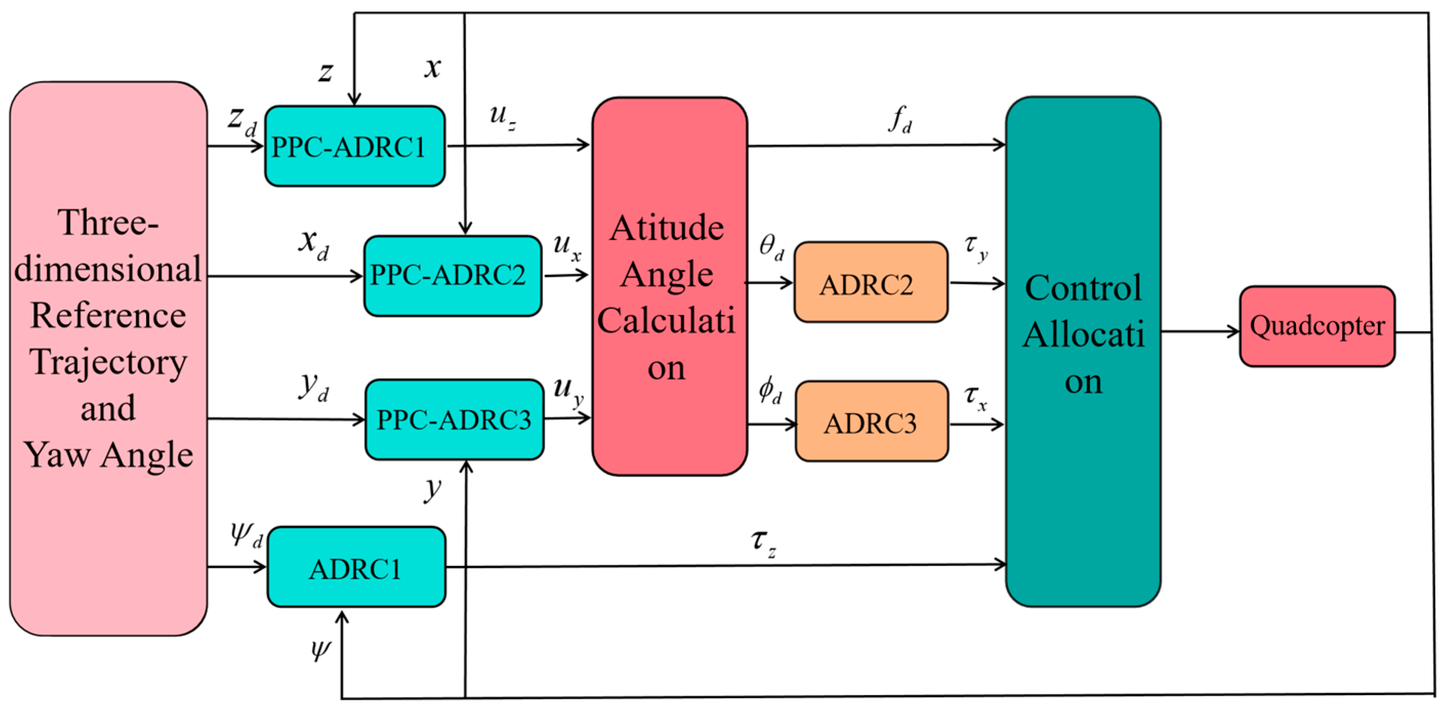
2.2. Quadcopter UAV Control System Design

In view of the underactuated characteristics of the quadrotor UAV, it is divided into four independent control channels: an $Z$-axis altitude channel, a cascade channel $X-\theta$, another cascade channel $Y-\varphi$, and a yaw channel $\psi$. The altitude and yaw channels are controlled by control inputs $f^d$ and control inputs ${\tau }_2$, respectively, while the cascade pitch $X-\theta$ and roll $Y-\varphi$ channels are controlled by control inputs ${\tau }_y$ and ${\tau }_x$. The specific control scheme is shown in Figure 2.

(1)

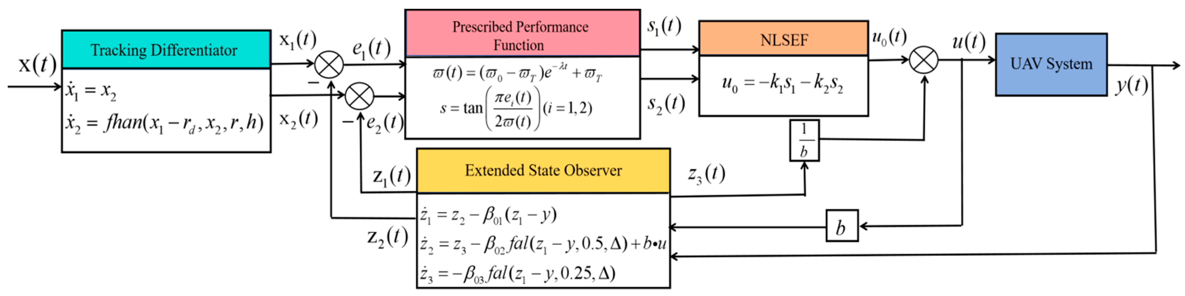
ADRC design with preset performance for the outer loop

In Figure 2, the quadrotor UAV position loops are all controlled by the PPC-ADRC controller (ADRC controller with preset performance), which includes the TD (differential tracker), the ESO (extended state observer), and the feedback control law in the PPC-ADRC controller. Among them, the TD (differential tracker) and ESO (extended state observer) are defined in this study as shown in Equations (3) and (4).

$$\left\{\begin{array}{c}{\dot{x}}_{1i}=x_{2i}\\ {\dot{x}}_{2i}=fhan(x_{1i}-r_{di},x_{2i},r_i,h)\end{array}\right.$$

(3)

In the TD (differential tracker), $r_{di}$ represents the reference input datum and $x_{1i}$ is the tracking signal output, while $x_{2i}$ characterises its first-order differential signal; the adjustment coefficients $r_i$ determine the convergence rate of the differential tracker (TD), and the size of the filtering parameter $h$ is the same as the time step of the system, where the fhan function is defined as follows:

$$\left\{\begin{array}{c}d=r_i{h}^2\\ a_0=h{x}_{2i}\\ y=x_{1i}-r_{di}+a_0\\ a_1=\sqrt{d(d+8\left|y\right|)}\\ a_2=a_0+\mathrm{sgn}(y){\displaystyle \frac{a_1-d}{2}}\\ s_y={\displaystyle \frac{\left[sign(y+d)-sign(y-d)\right]}{2}}\\ a=(a_0+y-a_2)s_y+a_2\\ s_a={\displaystyle \frac{\left[sign(a+d)-sign(a-d)\right]}{2}}\\ fhan=r_i({\displaystyle \frac{a}{d}}-sign(a)s_a-r_{i}sign(a))\end{array}\right.$$

In a complex ESO (extended state observer), the gain coefficients ${\beta }_{01},{\beta }_{02},{\beta }_{03}$ affect the observation performance by weighting the dynamic response of each error channel. The control inputs $u_i$ act on the dynamic equations of the observer through the control law gain coefficients $b_i$, forming a closed-loop correction to the system excitation signal.

$$\left\{\begin{array}{c}{\dot{z}}_{1i}=z_{2i}-{\beta }_{01}(z_{1i}-y_i)\\ {\dot{z}}_{2i}=z_{3i}-{\beta }_{02}fal(z_{1i}-y_i,0.5,\mathrm{\Delta })+b_i\cdot u_i\\ {\dot{z}}_{3i}=-{\beta }_{03}fal(z_{1i}-y_i,0.25,\mathrm{\Delta })\end{array}\right.$$

(4)

Combining the outputs of the differential tracker and the extended state observer, we can define the controller error as:

$$\left\{\begin{array}{c}{e}_{1i}=x_{1i}-z_{1i}\\ e_{2i}=x_{2i}-z_{2i}\end{array}\right.$$

(5)

where $e_{1i}$ denotes the difference between the output of the TD (differential tracker) $x_{1i}$ and the first-order estimate of the system state $z_{1i}$ by the ESO, and $e_{2i}$ is the difference between the output of the TD (differential tracker) $x_{2i}$ and the second-order estimate of the system state $z_{2i}$ by the ESO.

In order to ensure the dynamic and steady-state performance of the system, we use a preset performance function $\varpi (t)$ to constrain the error $e_{1i}$, so that $e_{1i},e_{2i} < \varpi (t)$. The preset performance function is defined as follows:

$${\varpi }_z(t)=({\varpi }_{z0}-{\varpi }_{zT})e^{-{\lambda }_{2}t}+{\varpi }_{zT}$$

(6)

where the initial parameter ${\varpi }_0$ denotes the initial tolerance range of the system error, and ${\varpi }_T$ is the residual error threshold when the system enters the steady-state phase while $\underset{x\to \infty }{\lim }\varpi \left(t\right)={\varpi }_T$ is satisfied. The function constructs a time-varying funnel-type performance envelope through the exponential contraction mechanism of ${\varpi }_0$ to ${\varpi }_T$.

In order to solve the problem of the restricted control error of the restricted preset performance and simplify the design of the control feedback law, we made the conversion of restricted error $e_{1i}$, $e_{2i}$, so that it is converted to the unbounded error $s_{1i},s_{2i}$. This paper defines the error conversion function as:

$$s=\tan \left({\displaystyle \frac{\pi e}{2\varpi \left(t\right)}}\right)$$

(7)

The control feedback law $u_{0i}=-k_1{s}_{1i}-k_2{s}_{2i}$ is designed for the unbounded error $s_{1i},s_{2i}$ and the final controller output $u_i=u_{0i}-{\displaystyle \frac{z_{3i}}{b_i}}$ is obtained after adding the perturbation compensation, where $k_1,k_2$ denotes the control feedback law gain and $b_i$ denotes the control law gain for perturbation compensation.

In summary, the structure of the final PPC-ADRC controller is shown in Figure 3:

(2)

Quadrotor kinematic decoupling and dynamic command mapping

In order to meet the design requirements of the hierarchical control system of the multi-rotor vehicle, this paper constructs the outer-loop position control of three axes (x,y,z), as shown in Figure 4, which adopts the pre-programmed performance self-resistant controller (PPC-ADRC), and its outputs $u_x,u_y,u_z$ are mapped by the under-driven kinematic model of the quadrotor, which generates the reference commands for the inner-loop attitudes. In the specific realisation, the vertical channel (z-axis) outer loop generates the total lift control quantity $f_d$ through the output $u_z$; the lateral plane (x- and y-axes) outer-loop output $u_x,u_y$ is decoupled into the reference trajectory of the roll angle ${\varphi }_d$ and the pitch angle ${\theta }_d$ through the constructed decoupling Equation (8) [16], which is shown in the dynamic decoupling Equation (8).

$$\left\{\begin{array}{c}{f}_d=mg+{\displaystyle \frac{m{u}_z}{\cos \varphi \cos \theta }}\\ {\varphi }_d=\arcsin ({\displaystyle \frac{m{u}_y\cos \psi -m{u}_x\sin \psi }{f_d}})\\ {\theta }_d=\arcsin ({\displaystyle \frac{m{u}_y\cos \psi -m{u}_x\sin \psi }{f_d}})\end{array}\right.$$

(8)

When the system satisfies the small angle assumption ($\varphi \approx 0,\theta \approx 0$) and the heading angle value is set to ${\psi }_d=0$, the non-linear coupling term in the dynamic decoupling Equation (8) can be linearised into the simplified model shown in Equation (9). This simplified model significantly reduces the computational complexity of the attitude control loop.

$$\left\{\begin{array}{l}{\varphi }_d={\displaystyle \frac{m{u}_y}{f_d}}\\ {\theta }_d={\displaystyle \frac{m{u}_x}{f_d}}\end{array}\right.$$

(9)

(3)

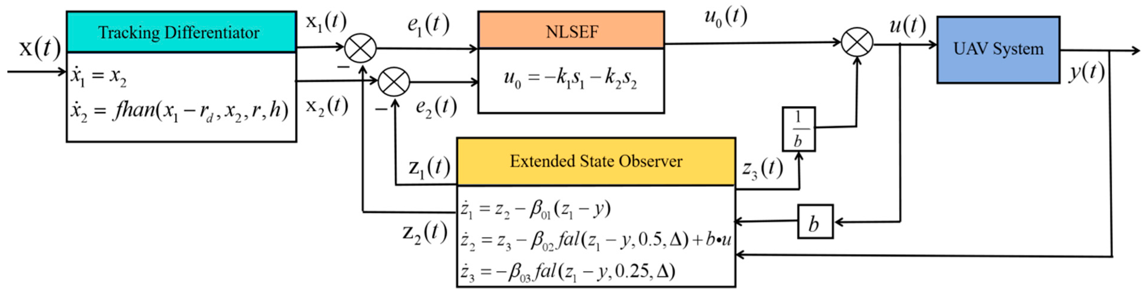
Inner-loop ADRC controller design

The core components of the inner-loop ADRC controller are the same as the outer-loop preset performance ADRC principle, but the inner loop uses the original error to construct a linear error feedback mechanism $u_0=k_p{e}_{1i}+k_d{e}_{2i}$ with $u_i={\displaystyle \frac{u_{0i}-z_{2i}}{b_i}}$, discarding the constraints of the preset performance function in the outer loop, and the specific structure of its controller is shown in Figure 4.

3. Crested Porcupine Optimiser (CPO) Principle and Improvements: Integration with ADRC

In this study, the crown porcupine optimisation (CPO) algorithm is introduced into the self-adjoint control (ADRC) parameter tuning and its population reduction strategy (CPR) is improved. Simulation experiments verify the advantages of the improved CPO in ADRC parameter tuning.

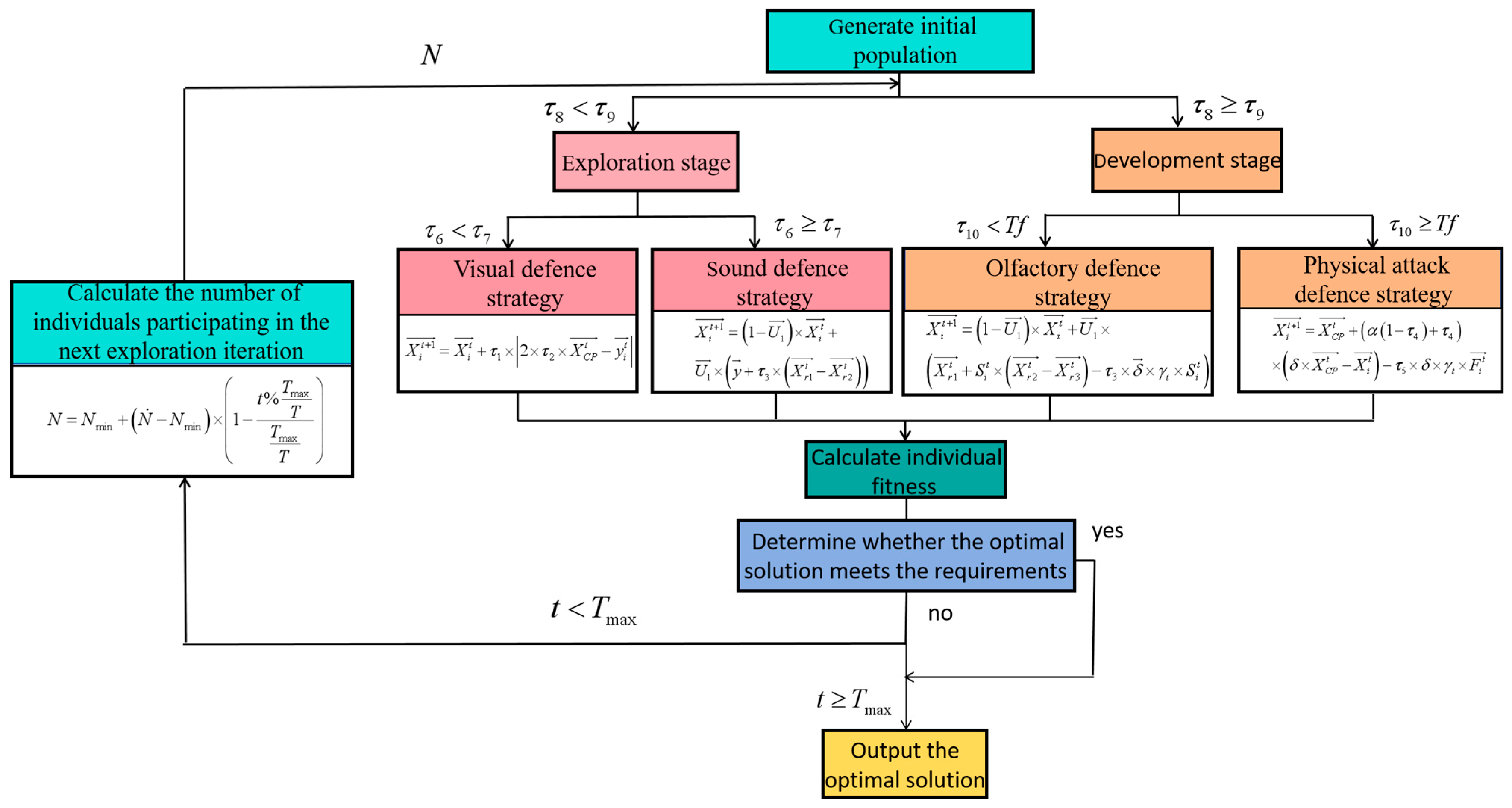
3.1. Crested Porcupine Optimiser (CPO) Principle

The crested porcupine optimiser (CPO) is a novel meta-heuristic algorithm inspired by the various defensive behaviours of the crested porcupine in nature, which contains 4 different protective mechanisms: visual, auditory, olfactory and physical attacks to recognise the aggressiveness of alien species. As shown in Figure 5, this diagram represents the whole process of the CPO algorithm.

(1)

Population initialisation

Similar to most meta-heuristic population algorithms, the initial population search process for the CPO is:

$$\overrightarrow{X_i}=\overrightarrow{L}+\overrightarrow{r}\times \left(\overrightarrow{U}-\overrightarrow{L}\right)\left|i=\right.1,2,\mathrm{\dots },N^{\prime }$$

(10)

where the population size $N\prime$ indicates the number of individuals, $\overrightarrow{X_i}$ is the i-th candidate solution in the search space, $\overrightarrow{L}$ and $\overrightarrow{U}$ are the lower and upper boundaries of the search range, respectively, and $\overrightarrow{r}$ is a vector.

(2)

Division of the exploration phase

In the figure, according to the comparison results of generating random numbers ${\tau }_8$ and ${\tau }_9$, decide whether its next step is to enter the exploration phase or the development phase [15].

If ${\tau }_8$ < ${\tau }_9$, enter the exploration stage. At this time, the algorithm focuses on finding potential solutions in a larger search space based on the relationship between the generated random numbers, chooses the visual defence strategy or the sound defence strategy, and simulates the defence behaviour of the crown porcupine in the natural environment to search for a new solution space.

In the exploration stage, if ${\tau }_6 < {\tau }_7$, a visual defence strategy is adopted. At this time, for the crown porcupine, the alien species has two possibilities: to continue to approach or to stay away. A normal distribution is used to generate random values and judge the size to simulate these two situations. If its absolute value is less than 1, it will continue to approach the crown porcupine, and vice versa, to stay away. The mathematical model is as follows:

$$\overrightarrow{X_i^{t+1}}=\overrightarrow{X_i^t}+{\tau }_1\times \left|2\times {\tau }_2\times \overrightarrow{X_{\mathrm{CP}}^{\mathrm{t}}}-\overrightarrow{y_{\mathrm{i}}^{\mathrm{t}}}\right|$$

(11)

where $\overrightarrow{X_{CP}^t}$ is the best obtained solution for the function evaluation $t$, $\overrightarrow{y_{\mathrm{i}}^{\mathrm{t}}}$ is a vector generated in the midst between the current CP and a CP selected randomly from the population to represent the position of a predator at iteration $t$, ${\tau }_1$ is a random number based on the normal distribution, and ${\tau }_2$ is a random value in the interval of $\left[0,1\right]$. The mathematical formula $\overrightarrow{y_{\mathrm{i}}^{\mathrm{t}}}$ represents the vector generated between the current individual and a random individual.

In the exploration stage, if ${\tau }_6\ge {\tau }_7$, an acoustic defence strategy is adopted. The sound defence strategy unfolds when the alien species approaches a certain degree, and the crown porcupine starts to make noise to warn the alien species, and the sound will increase with the shortening of the distance, and the mathematical model is as follows:

$$\overrightarrow{X_i^{t+1}}=\left(1-\overrightarrow{U_1}\right)\times \overrightarrow{X_i^t}+\overrightarrow{U_1}\times \left(\overrightarrow{y}+{\tau }_3\times \left(\overrightarrow{X_{r1}^t}-\overrightarrow{X_{r2}^t}\right)\right)$$

(12)

where $r1$ and $r2$ are two random integers between $\left[1,N\right]$, and ${\tau }_3$ is a random value generated between $0$ and $1$.

If ${\tau }_8$ ≥ ${\tau }_9$, then enter the development phase, focusing on the optimisation of the existing better solution.

Development phase: based on the comparison of the generated random numbers ${\tau }_{10}$ and parameters $Tf$, the olfactory defence strategy or the physical attack defence strategy is selected to refine and improve the current solution locally.

In the development stage, if ${\tau }_{10} < Tf$, the odour defence strategy is selected. At this time, the crown porcupine secretes an odour in the surrounding area to play a warning role, and its mathematical model is as follows:

$$\overrightarrow{X_i^{t+1}}=\left(1-\overrightarrow{U_1}\right)\times \overrightarrow{X_i^t}+\overrightarrow{U_1}\times \left(\overrightarrow{X_{r1}^t}+S_i^t\times \left(\overrightarrow{X_{r2}^t}-\overrightarrow{X_{r3}^t}\right)-{\tau }_3\times \overrightarrow{\delta }\times {\gamma }_t\times S_i^t\right)$$

(13)

where $r_3$ is a random number between $\left[1,N\right]$, $\delta$ is a parameter used to control the search direction, $\overrightarrow{X_i^t}$ is the position of the $ith$ individual at iteration $t$, ${\gamma }_t$ is the defence factor, ${\tau }_3$ is a random value within the interval [0, 1], and ${S^t}_i$ is the odour diffusion factor.

In the development stage, if ${\tau }_{10}\ge Tf$, a physical attack defence strategy is chosen. At this time, the crown porcupine launches a physical attack on the other party, and its mathematical model is as follows:

$$\overrightarrow{X_i^{t+1}}=\overrightarrow{X_{CP}^t}+\left(\alpha \left(1-{\tau }_4\right)+{\tau }_4\right)\times \left(\delta \times \overrightarrow{X_{CP}^t}-\overrightarrow{X_i^t}\right)-{\tau }_5\times \delta \times {\gamma }_t\times \overrightarrow{F_i^t}$$

(14)

where $\overrightarrow{X_{CP}^t}$ is the best obtained solution and represents the CP, $\overrightarrow{X_i^t}$ is the position of the $ith$ individual at iteration $t$ and represents the position’s predator, $\alpha$ is a convergence speed factor, ${\tau }_4$ is a random value within the interval $\left[0,1\right]$, and $\overrightarrow{F_i^t}$ is the average force of the CP that affected the $ith$ predator.

After finding the fitness, determine whether the current optimal solution meets the preset requirements. If so, the algorithm ends and outputs the optimal solution; if not, then continue to iterate. After each iteration, the number of individuals in the population participating in the search next time is adjusted according to the number of iterations, and its specific adjustment formula is as follows:

$$N=N_{\min }+\left(N\prime -N_{\min }\right)\times \left(1-\left({\displaystyle \frac{t\%\frac{T_{\max }}{T}}{\frac{T_{\max }}{T}}}\right)\right)$$

(15)

This formula $N_{\min }$ represents the minimum population size, meaning that the population size will never fall below this minimum value, and $N^{\prime }$ represents the maximum population size. The loop variable for the second loop is $T$.

3.2. Optimisation Algorithm Design

(1)

Defects of classical crown porcupine optimisation

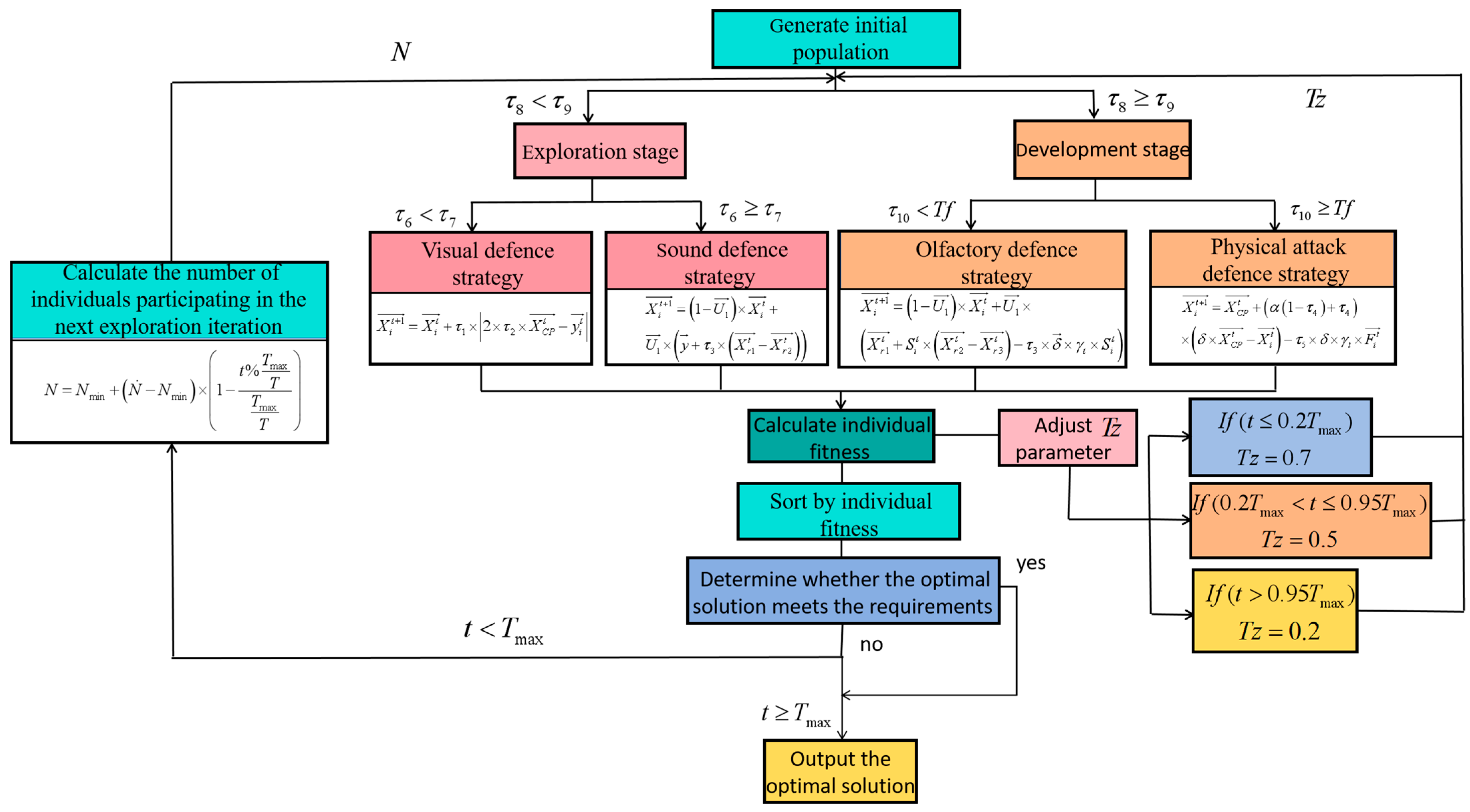
The classical CPO algorithm adopts a fixed elimination mechanism based on the descending order of individual numbers in the dynamic reduction phase of the population size of the cyclic population reduction, which does not adequately consider the impact of individual fitness differences on the convergence efficiency of the algorithm.

(2)

Improvement method

To address the above problems, this study proposes an improved CPO algorithm, which optimises the distribution of the selection pressure during population iteration by introducing a directed elimination strategy based on an individual fitness assessment. The flowchart of the improved CPO algorithm is shown in Figure 6.

In the figure, we can find that compared with the original CPO algorithm flowchart, this paper implements two improvement measures:

(a)

fitness-based individual ranking operator is constructed to reorder individuals based on their fitness values $L\left(x_i\right)$, and the individuals are sorted in ascending order $L\left(x_1\right)\le L\left(x_2\right)\le \mathrm{\dots }\le L\left(x_{N_{\max }}\right)$ to ensure that low-fitness individuals are prioritised for elimination when adjusting the number of individuals in the population in each round of the cycle, thus enhancing the selection pressure.

(b)

The generation of random numbers ${\tau }_9$ in the original algorithm is changed to a time-varying deterministic threshold $T_z$:

$$\left\{\begin{array}{l}0.7,{\displaystyle \frac{t}{T_{\max }}}\le 0.2\\ 0.5,0.2<{\displaystyle \frac{t}{T_{\max }}}\le 0.95\\ 0.2,{\displaystyle \frac{t}{T_{\max }}}>0.95\end{array}\right.$$

(16)

where $t$ is the current number of iterations of the algorithm, and $T_{\max }$ is the maximum number of iterations. The design follows the principle of the “exploration–exploitation trade-off”: at the beginning, the high value $T_z$ promotes a global search to break through the local optimum; in the middle, the equilibrium state maintains the diversity of the population; and at the end, the low value $T_z$ accelerates the local convergence, which is in line with the demand for dynamic adjustment of the algorithm optimisation process.

It allows this paper to artificially balance the proportion of the exploration phase (finding new solution spaces) and the development phase (optimising existing solutions) in the CPO algorithm.

3.3. Integration of Active Disturbance Rejection Control (ADRC) and Crested Porcupine Optimiser Algorithm (CPO)

(1)

Combination of ADRC and ICPO

In the self-resilient control (ADRC) system, the cumulative tracking error is used as a fitness function to evaluate the performance, considering the accurate evaluation of the global performance of the parameters, and the performance evaluation function used is

$$E_{ISE}={\displaystyle \int \begin{array}{l}{t}_1\\ t_0\end{array}}{e}^2\left(t\right)dt$$

(17)

where a high value $E_{ISE}$ indicates poor performance and a low value $E_{ISE}$ indicates good performance.

The crowned porcupine optimisation (ICPO) algorithm was used for the ADRC parameter optimisation with the objective of minimising the fitness function $E_{ISE}$. The ICPO has a time-varying selection characteristic and uses visual and acoustic defence strategies to find better parameters in the exploration phase, and it uses scent and physical attack defence strategies to optimise the existing parameters in the development phase, as well as using the boundary bounce mechanism to deal with the out-of-bounds individuals.

When iterating, the ADRC parameters are updated according to the group fitness, the global and local searches are balanced, the 24-dimensional parameters of the ADRC control framework position loop (3 independent outer-loop preset performance channels) and attitude loop (3 channels) are adjusted, and the TD gain and ESO observer parameters are adjusted, so as to improve the efficiency and accuracy of the ADRC parameter optimisation [19,20]. In summary, the final integration pseudocode is as follows:

Pseudocode for a quadrotor PPC-ADRC + ADRC control system with CPO parameter tuning Input: reference trajectory instruction ${\chi }_{ref}=\left[x_{ref}{y}_{ref}{z}_{ref}\right]$, desired yaw angle ${\psi }_d$ Output: angle of attitude $\mathrm{\Phi }=\left[\varphi \theta \psi \right]$, control input $u(t)$ BEGIN 1. Initialise system parameters: $L_a$, $L_p$, $L_q$, inertia matrix $I$, quality $m$, arm length $L$, thrust coefficient $k_t$, drag coefficient $k_d$ 2. ICPO parameter tuning process                 Define the vector of optimisation parameters:                 $P=\left[\begin{array}{lllllll}{b}_{pos}& {\beta }_{01,pos}& {\beta }_{02,pos}& {\beta }_{03,pos}& k_{1,pos}& k_{2,pos}& \cdot \cdot \cdot \\ b_{att}& {\beta }_{01,att}& {\beta }_{02,att}& {\beta }_{03,att}& k_{1,att}& k_{2,att}& \cdot \cdot \cdot \end{array}\right]$                 define upper and lower bounds: $\left[\begin{array}{cc}lb& ub\end{array}\right]$                 Define CPO optimisation parameters: population size:$Pop\_size$, maximum number of iterations $T_{\max }$, dimension $\dim$.                 Define fitness function: $f(P)=w_{error}\cdot {\displaystyle \sum _{t=0}^{t_{\max }}error}$              CPO algorithm:                 Initialise population $Pop\_size$, $\dim$                 Evaluate initial population fitness: $fitness(Pop\_size)$                 Update global best solution $Gb\_Sol$ and global best fitness $Gb\_Fit$                 For $t=0$ to $T_{\max }$                       For $i=0$ to $Pop\_size$                             If ${\tau }_8<Tz$:                                  Exploration stage:                                       If ${\tau }_6<{\tau }_7$:                             visual defence strategy: $\overrightarrow{X_i^{t+1}}=\overrightarrow{X_i^t}+{\tau }_1\times \left|2\times {\tau }_2\times \overrightarrow{X_{\mathrm{CP}}^{\mathrm{t}}}-\overrightarrow{y_{\mathrm{i}}^{\mathrm{t}}}\right|$                                       If ${\tau }_6\ge {\tau }_7$:                                  sound defence strategy: $\overrightarrow{X_i^{t+1}}=\left(1-\overrightarrow{U_1}\right)\times \overrightarrow{X_i^t}+\overrightarrow{U_1}\times \left(\overrightarrow{y}+{\tau }_3\times \left(\overrightarrow{X_{r1}^t}-\overrightarrow{X_{r2}^t}\right)\right)$                       If ${\tau }_8\ge Tz$:                            development stage:                                 If ${\tau }_{10}<Tf$:                            olfactory defence strategy:                            $\overrightarrow{X_i^{t+1}}=\left(1-\overrightarrow{U_1}\right)\times \overrightarrow{X_i^t}+\overrightarrow{U_1}\times \left(\overrightarrow{X_{r1}^t}+S_i^t\times \left(\overrightarrow{X_{r2}^t}-\overrightarrow{X_{r3}^t}\right)-{\tau }_3\times \overrightarrow{\delta }\times {\gamma }_t\times S_i^t\right)$                                 If ${\tau }_{10}\ge Tf$:                                      Physical attack defence strategy:                                      $\overrightarrow{X_i^{t+1}}=\overrightarrow{X_{CP}^t}+\left(\alpha \left(1-{\tau }_4\right)+{\tau }_4\right)\times \left(\delta \times \overrightarrow{X_{CP}^t}-\overrightarrow{X_i^t}\right)-{\tau }_5\times \delta \times {\gamma }_t\times \overrightarrow{F_i^t}$                     Boundary handling                     evaluate the fitness of the new solution                     update the individual best solution and the global best solution                   End For                   Update population size $Pop\_size$: $N=N_{\min }+\left(N\prime -N_{\min }\right)\times \left(1-\left({\displaystyle \frac{t\%\frac{T_{\max }}{T}}{\frac{T_{\max }}{T}}}\right)\right)$            End For            optimal parameter set $P_{best}=Gb\_Sol$ 3. Initialise the controller using the optimal parameters $P_{best}$ position control parameter: $b_{pos},{\beta }_{01,pos},{\beta }_{02,pos},{\beta }_{03,pos},k_{1,pos},k_{2,pos},\mathrm{\dots }$            posture control parameter: $b_{att},{\beta }_{01,att},{\beta }_{02,att},{\beta }_{03,att},k_{1,att},k_{2,att},\mathrm{\dots }$           Initialise the preset performance function       parameters: ${\varpi }_0=15,{\varpi }_T=0.5,\lambda =0.01$            initial state: $x_1=0,x_2=0,z_1=0,z_2=0,z_3=0,u_{prev}=0$ 4. Definition of a non-linear function             Predefined performance functions: $\varpi (t)=({\varpi }_0-{\varpi }_T)e^{-\lambda t}+{\varpi }_T$            Error conversion function definition: $s=\tan ({\displaystyle \frac{\pi e}{2\varpi (t)}})$               $ftppf(e_1,e_2,{\varpi }_0,{\varpi }_T,\lambda ,t)=(\tan ({\displaystyle \frac{\pi e_1}{2\varpi (t)}}),\tan ({\displaystyle \frac{\pi e_1}{2\varpi (t)}}))$ 5. Start quadcopter tracking control loop               For $t=0$ to $t_{final}$               Obtain the desired states $x_d(t),y_d(t),z_d(t),{\psi }_d(t)$               Obtain the current states $x(t),v(t),\mathrm{\Phi }(t),\dot{\mathrm{\Phi }}(t)$               For $i=1$ to 3: //location tracking control               Corresponds to the x-, y-, and z-axes—Update the state of the tracking differentiator:                               $\left\{\begin{array}{c}{\dot{x}}_{1i}=x_{2i}\\ {\dot{x}}_{2i}=fhan(x_{1i}-r_{di},x_{2i},r_i,h)\end{array}\right.$                               Update the expansion status observer (ESO) status:                                $\left\{\begin{array}{c}{\dot{z}}_{1i}=z_{2i}-{\beta }_{01}(z_{1i}-y_i)\\ {\dot{z}}_{2i}=z_{3i}-{\beta }_{02}fal(z_{1i}-y_i,0.5,\mathrm{\Delta })+b_i·u_i\\ {\dot{z}}_{3i}=-{\beta }_{03}fal(z_{1i}-y_i,0.25,\mathrm{\Delta })\end{array}\right.$                               Apply preset performance function transformation:                               $\begin{array}{l}{e}_1=x_{1i}-z_{1i}\\ e_2=x_{2i}-z_{2i}\end{array}$                               $(s_1,s_2)=ftppf(e_1,e_2,{\varpi }_0,{\varpi }_T,\lambda ,t)$                               computational control law:                               $\begin{array}{l}{u}_0=k_{1i}\cdot s_1+k_{2i}\cdot s_2\\ u=u_0-{\displaystyle \frac{z_{3i}}{b_i}}\end{array}$                               $u=u_x,u_y,u_z;i=1,2,3$                          End For                          Calculate desired roll and pitch angles:                      $\begin{array}{l}{\varphi }_d=\arcsin ({\displaystyle \frac{m{u}_y\cos \psi -m{u}_x\sin \psi }{f_d}})\\ {\theta }_d=\arcsin ({\displaystyle \frac{m{u}_y\cos \psi -m{u}_x\sin \psi }{f_d}})\end{array}$            For $i=1$ to 3: //Posture control cycle calculation                      Update the pose tracker differentiator state:                      $\left\{\begin{array}{c}{\dot{x}}_{1i}=x_{2i}\\ {\dot{x}}_{2i}=fhan(x_{1i}-r_{di},x_{2i},r_i,h)\end{array}\right.$                      Update the posture expansion state observer:                      $\left\{\begin{array}{c}{\dot{z}}_{1i}=z_{2i}-{\beta }_{01}(z_{1i}-y_i)\\ {\dot{z}}_{2i}=z_{3i}-{\beta }_{02}fal(z_{1i}-y_i,0.5,\mathrm{\Delta })+b_i\cdot u_i\\ {\dot{z}}_{3i}=-{\beta }_{03}fal(z_{1i}-y_i,0.25,\mathrm{\Delta })\end{array}\right.$                      calculate posture control:                      $\begin{array}{l}{e}_1=x_{1i}-z_{1i}\\ e_2=x_{2i}-z_{2i}\end{array}$                      $\begin{array}{l}{u}_0=k_{1i}\cdot e_1+k_{2i}\cdot e_2\\ u=u_0-{\displaystyle \frac{z_{3i}}{b_i}}\end{array}$                      $u=u_{att}=u_{\varphi },u_{\theta },u_{\psi };i=1,2,3$                      (Note: The PPC-ADRC + ADRC is not required for the yaw angle’s control input $u_{\psi }$. As it is only a first-order system, the yaw angle $\psi$ can be directly controlled by the inner-loop ADRC controller, which outputs $u_{\psi }$.)              End For        //Final control input calculation              $\begin{array}{l}{u}_1=m(g+u_z)\\ u_2=I\cdot u_{att}\end{array}$              $u=\left[\begin{array}{l}{u}_1\\ u_2\end{array}\right]$        Calculation of the motor speed from thrust and torque:         $F={(TM)}^{-1}\cdot u$         $w_i=\sqrt{{\displaystyle \frac{F_i}{k_t}}},i=1,2,3,4$        Real-time assessment of the quadrotor response        Apply control inputs $w_i$ to the motors        Measure and record state variables, errors and performance indicators     End For END

(2)

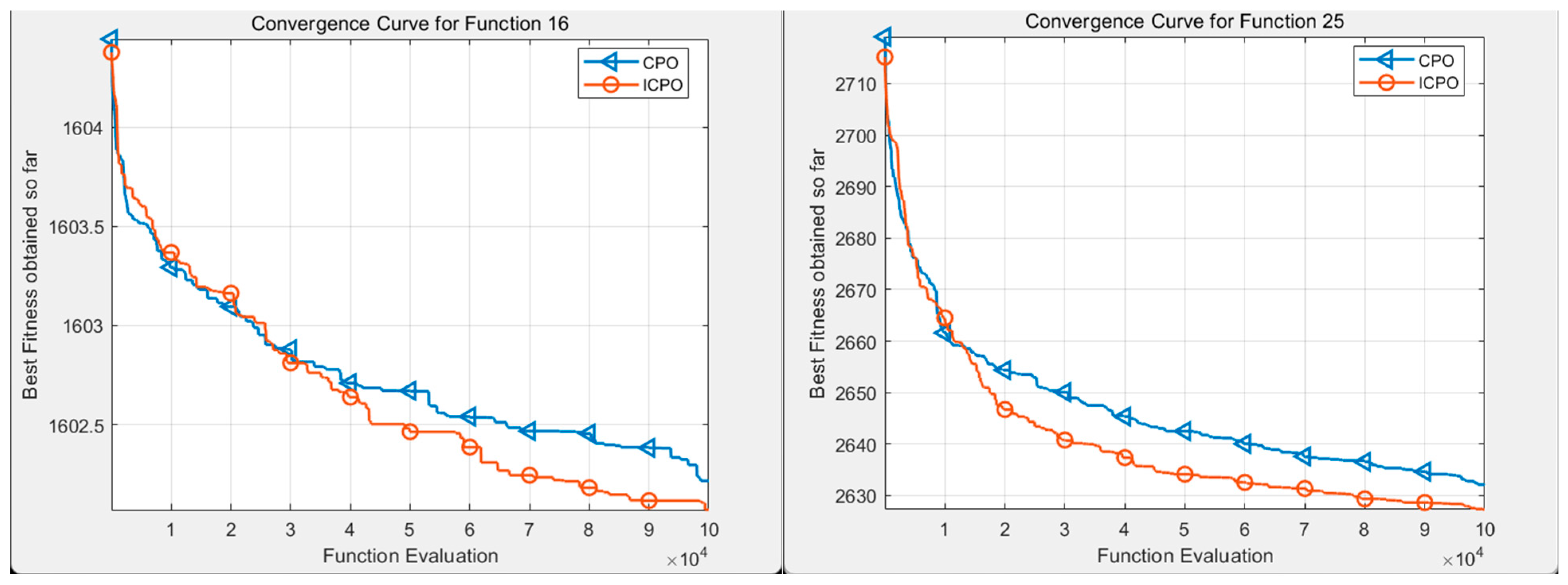
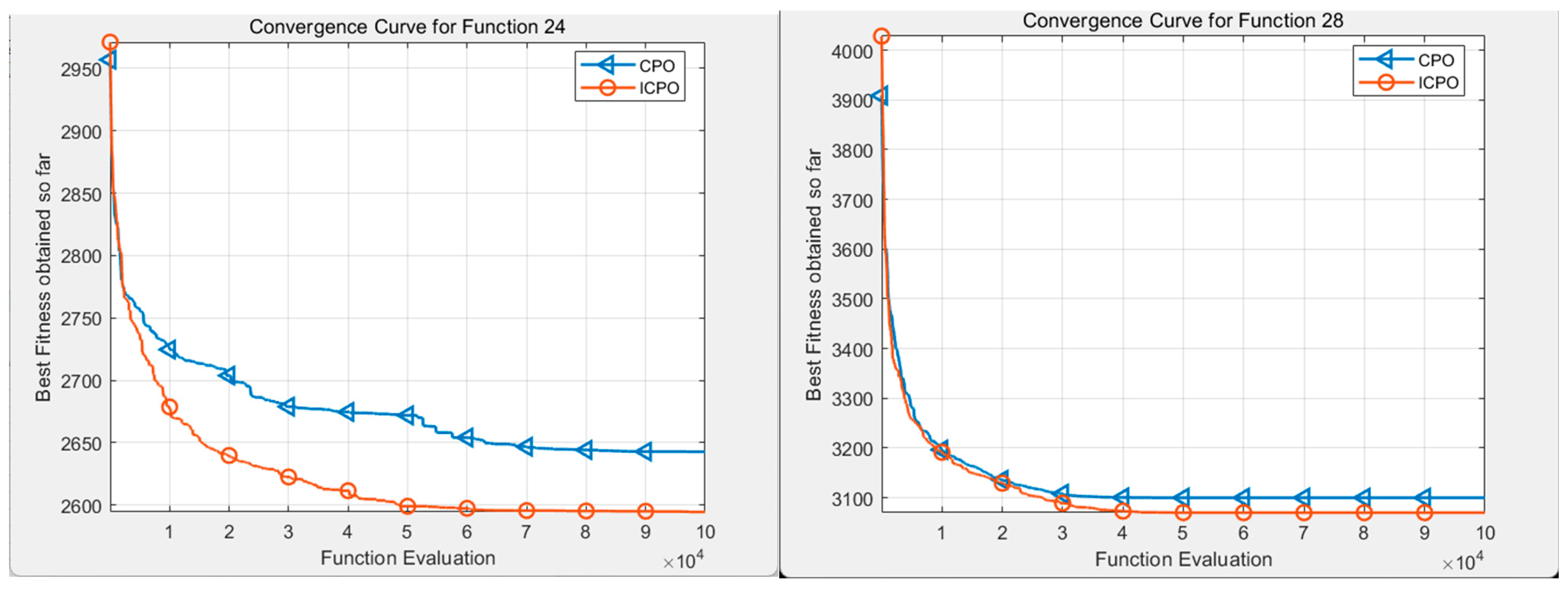
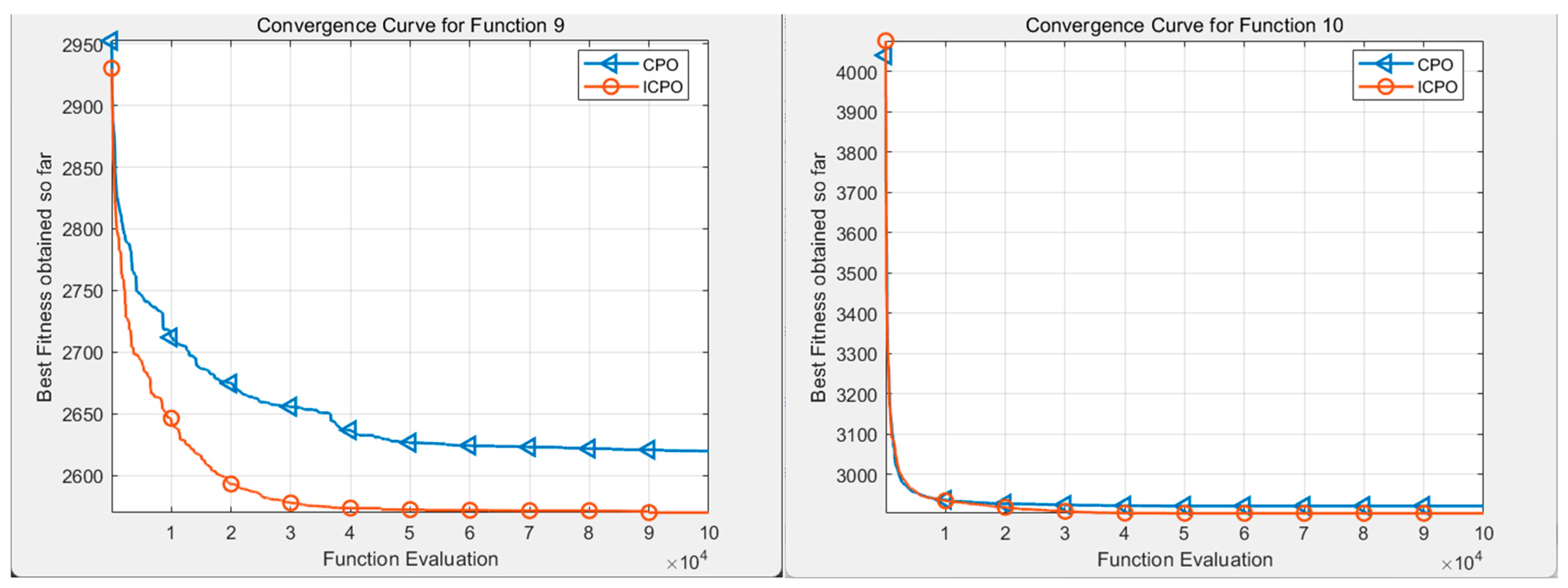
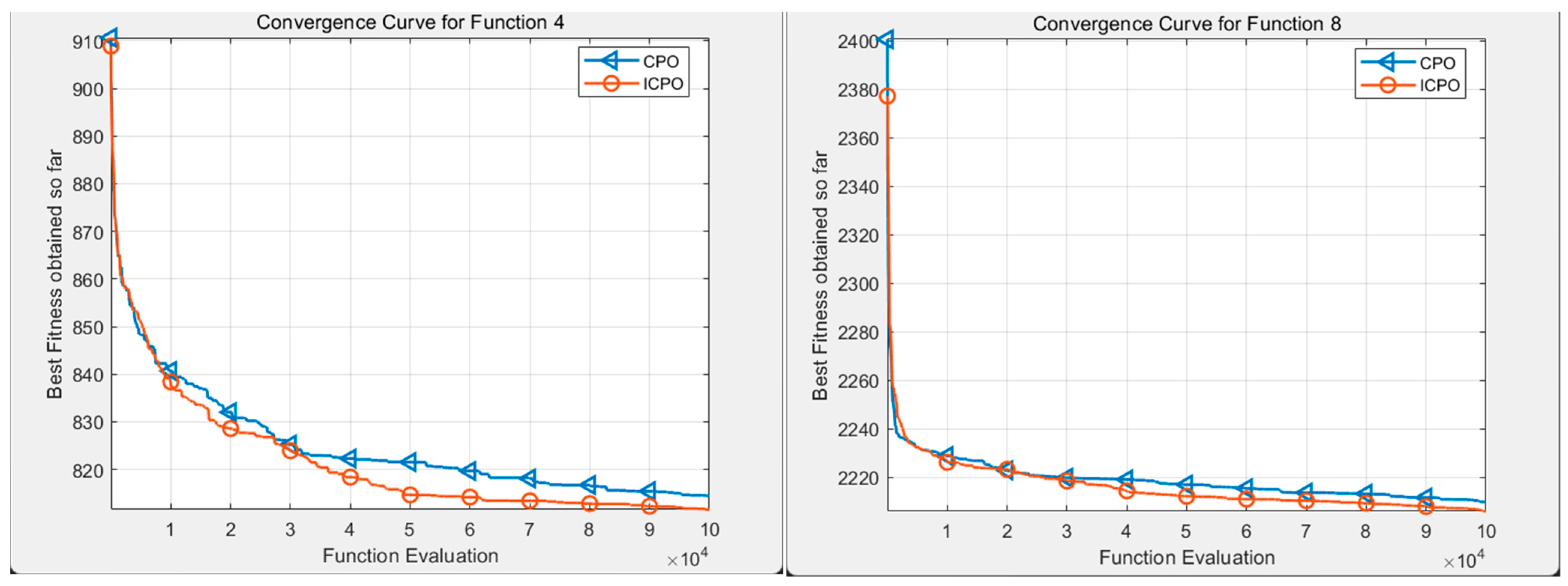
Improved CPO(ICPO) vs. classical CPO algorithms on CEC benchmarks

This section aims to investigate the CPO with ICPO in solving four challenging CEC benchmarks (CEC2017, CEC2014, CEC2020 and CEC2022). All the algorithms were implemented in MTALB R2019a, in which $T_{\max }$ was limited to 100,000 for all the CEC benchmarks, and each algorithm was run independently 20 times. The population sizes of these algorithms were set as suggested in the original reference, while the suggested population size for CPO was set to 130.

(a)

Comparative analysis of the CEC2014 benchmark test

The CPO algorithm and the winning algorithm in terms of the CEC competition were run independently 30 times, respectively, and the fitness values obtained by each algorithm on the CEC2014 test function set were statistically analysed. The specific indexes include the mean (Avg), standard deviation (SD) and rank (Rank), and the relevant results are summarised in Appendix A,

Table A1. Comparative analysis of CPO algorithm and CEC competition-winning algorithm on CEC2014 benchmark test functions.

Function_ID	Avg Fitness Rank (CPO)	Avg Fitness Rank (ICPO)	SD Fitness Rank (CPO)	SD Fitness Rank (ICPO)
1	2	1	2	1
2	2	1	1	2
3	2	1	2	1
4	2	1	1	2
5	1	2	1	2
6	2	1	2	1
7	2	1	2	1
8	2	1	2	1
9	2	1	2	1
10	2	1	1	2
11	1	2	2	1
12	2	1	1	2
13	2	1	1	2
14	2	1	2	1
15	2	1	1	2
16	2	1	1	2
17	2	1	1	2
18	2	1	1	2
19	2	1	2	1
20	2	1	2	1
21	2	1	2	1
22	2	1	2	1
23	1.5	1.5	1.5	1.5
24	2	1	1	2
25	2	1	1	2
26	2	1	1	2
27	1	2	1	2
28	1	2	2	1
29	2	1	1	2

.

In terms of the average fitness ranking, among the 29 test functions, the ICPO algorithm ranks first in the average fitness ranking on 24 of them. It indicates that under the test scenarios of these functions, the average fitness of the ICPO algorithm is significantly better than that of the CPO algorithm. The CPO algorithm has a leading average fitness ranking on 5 functions (with function IDs of 5, 11, 27, and 28), performing more excellently than the ICPO algorithm. For the function with function ID 23, the average fitness rankings of the CPO and ICPO algorithms are the same, both being 1.5.

In terms of the fitness standard deviation ranking, the ICPO algorithm ranks first on 14 functions, which means that during the testing of these functions, the stability of its fitness (i.e., the standard deviation is relatively smaller) is better than that of the CPO algorithm. The CPO algorithm has a leading fitness standard deviation ranking on 13 functions, with a rank of 1, indicating that on these functions, the fitness stability of the CPO algorithm is stronger than that of the ICPO algorithm. For the function with function ID 23, the fitness standard deviation rankings of the CPO and ICPO algorithms are the same, both being 1.5.

The following Figure 7 shows a comparison of the convergence curves of the CPO and ICPO for F16 and F25

Overall, the ICPO algorithm significantly demonstrates superiority or strong competitiveness on 24 test functions because its average fitness ranking on these 24 functions is 1; it performs comparably to the CPO algorithm on 1 function (function ID 23); and it is only slightly inferior to the CPO algorithm on the remaining 4 functions. In summary, the ICPO algorithm demonstrates better performance than the CEC competition-winning algorithm on the vast majority of test functions in the CEC2014 benchmark test.

(b)

Comparative analysis of the CEC2017 benchmark test

For the CEC2017 benchmark test, the ICPO algorithm and the CPO algorithm were also run independently 30 times, and the adaptation values obtained by each algorithm were analysed in terms of the average adaptation, standard deviation, and ranking. The relevant results are shown in Appendix A,

Table A2. Comparative analysis of ICPO and CPO algorithms on CEC2017 benchmark test functions.

Function_ID	Avg Fitness Rank (CPO)	Avg Fitness Rank (ICPO)	SD Fitness Rank (CPO)	SD Fitness Rank (ICPO)
1	2	1	2	1
2	2	1	1	2
3	1	2	1	2
4	2	1	1	2
5	2	1	1	2
6	2	1	2	1
7	2	1	2	1
8	1	2	2	1
9	1.5	1.5	1.5	1.5
10	2	1	2	1
11	2	1	2	1
12	2	1	1	2
13	2	1	1	2
14	2	1	2	1
15	2	1	1	2
16	2	1	1	2
17	2	1	1	2
18	2	1	1	2
19	2	1	2	1
20	1	2	1	2
21	2	1	2	1
22	2	1	2	1
23	1.5	1.5	1.5	1.5
24	1	2	1	2
25	1	2	1	2
26	1	2	1	2
27	2	1	1	2
28	1	2	2	1
29	2	1	1	2

.

In the CEC2017 benchmark test, in terms of the average fitness ranking, among the 29 test functions, the ICPO algorithm ranked first (with a rank of 1) in the average fitness for 22 functions (such as those with function IDs 1, 4, 5, etc.), demonstrating its superiority over the CPO algorithm. The CPO algorithm, on the other hand, ranked first (with a rank of 1) in the average fitness for 5 functions with function IDs 3, 8, 20, 24, 25, and 26, outperforming the ICPO algorithm. For the functions with function IDs 9 and 23, the average fitness rankings of the two algorithms were the same, both being 1.5.

Regarding the fitness standard deviation ranking, the ICPO algorithm ranked first (with a rank of 1) for 13 functions, indicating that its fitness stability was better than that of the CPO algorithm. The CPO algorithm also ranked first (with a rank of 1) for 13 functions, showing that its fitness stability was superior to that of the ICPO algorithm in these functions. For the functions with function IDs 9 and 23, the fitness standard deviation rankings of the two algorithms were both 1.5.

The following Figure 8 shows the comparison of the convergence curves of the CPO and ICPO for F16 and F25.

Overall, the ICPO algorithm demonstrated superiority or competitiveness in 22 test functions, performed comparably to the CPO algorithm in 2 functions with function IDs 9 and 23, and was slightly inferior to the CPO algorithm in the remaining 5 functions. Moreover, the average value of the ranking scores of each algorithm in the table showed that the ICPO algorithm ranked first. In summary, the ICPO algorithm demonstrated better performance than the CPO algorithm on the vast majority of test functions in the CEC2017 benchmark.

(c)

Comparative Analysis of CEC2020 Benchmarks

In this subsection, experiments are carried out for the CEC2020 test suite, and the CPO algorithm and the CEC competition-winning algorithm are run independently 30 times, respectively. The obtained fitness values are statistically analysed, and the results are shown in Appendix A,

Table A3. Comparative analysis of CPO algorithm and CEC competition-winning algorithm on CEC2020 test suite.

Function_ID	Avg Fitness Rank (CPO)	Avg Fitness Rank (ICPO)	SD Fitness Rank (CPO)	SD Fitness Rank (ICPO)
1	1	2	1	2
3	2	1	1	2
4	2	1	2	1
5	2	1	1	2
6	2	1	1	2
7	1	2	2	1
8	2	1	2	1
9	1	2	2	1
10	2	1	2	1

.

In the analysis of the CEC2020 test suite, from the perspective of the average fitness ranking, among the 10 test functions, the ICPO algorithm ranked first in average fitness on 6 functions with function IDs 3, 4, 5, 6, 8, and 10, demonstrating a better average fitness than the CPO algorithm. For example, in the function with function ID 3, its advantage is obvious. The CPO algorithm ranked first in average fitness on 3 functions, with function IDs 1, 7, and 9 showing more outstanding performance. For instance, in the function with function ID 1, the result is prominent. In addition, for the function with function ID 4, although the ICPO algorithm ranked first, the performances of the two algorithms are close, with a small gap in average fitness levels.

In terms of the fitness standard deviation ranking, the ICPO algorithm ranked first on 4 functions with function IDs 7, 9, 1, and 3, indicating better fitness stability. For example, in the function with function ID 7, the fitness fluctuation is smaller. The CPO algorithm ranked first on 5 functions with function IDs 4, 5, 6, 8, and 10, showing stronger fitness stability. For example, in the function with function ID 5, the performance is more stable.

By synthesising the average fitness ranking and fitness standard deviation ranking, the ICPO algorithm has an advantage in 6 test functions, is close to the CPO in the function with function ID 4, and lags behind the CPO in 3 functions. It indicates that in the 10—10-function test of the CEC2020 test suite, the ICPO algorithm has considerable overall performance and certain competitiveness. The following Figure 9 compares the convergence curves of CPO and ICPO for F9 and F10.

Based on its excellent ranking performance on most of the test functions, the CPO algorithm can be classified as a high-performance optimisation algorithm, and the experimental results in this subsection further validate the high-performance property of the CPO algorithm.

(d)

Comparative Analysis of CEC2022 Benchmark

This subsection evaluates the performance of the newly released challenging benchmark CEC2022. The benchmark contains 12 test functions classified into four categories: single-peak, multi-peak, combined and hybrid. In Appendix A, Table A3 shows the results of the analysis of the fitness values obtained by each algorithm in 30 independent runs.

In the in-depth analysis of the CEC2022 benchmark test, from the perspective of the average fitness ranking, within the evaluation system of all 12 test functions, the ICPO algorithm achieved first place in the average fitness ranking for 10 functions with function IDs 1, 3, 4, 5, 6, 7, 8, 9, 10, and 12. This result strongly demonstrates that compared with the CPO algorithm, the ICPO algorithm can achieve a better average fitness level during the optimisation process of the above-mentioned functions. Especially, taking the function with function ID 1 as an example, its advantage is fully manifested. In contrast, the CPO algorithm only achieved first place in the average fitness ranking for two functions with function IDs 11 and 12, and in the function with function ID 11, its average fitness result is also quite outstanding.

From the dimension of the fitness standard deviation ranking, the ICPO algorithm won first place in the fitness standard deviation ranking for 6 functions with function IDs 1, 3, 4, 5, 6, 9, and 10, which fully indicates that the algorithm exhibits more excellent fitness stability on these functions, that is, its fitness fluctuation range is relatively smaller, with the function of function ID 1 as a typical example. The CPO algorithm, on the other hand, achieved first place in the fitness standard deviation ranking for 4 functions with function IDs 7, 8, 11, and 12, which means that under the test scenarios of these functions, the CPO algorithm shows stronger fitness stability.

By evaluating based on the dual indicators of the average fitness ranking and the fitness standard deviation ranking, the ICPO algorithm has established significant advantages in as many as 10 test functions and only lags behind the CPO algorithm in 2 functions. This data clearly shows that within the overall scope of the 12 functions covered by the CEC2022 test, the ICPO algorithm demonstrates strong competitiveness with its more outstanding comprehensive performance. The CPO algorithm only ranked first in the average fitness for 2 functions and first in the fitness standard deviation for 4 functions.

The following Figure 10 compares the convergence curves of the CPO and ICPO for F4 and F8.

Overall, the ICPO algorithm has demonstrated excellent performance in the vast majority of functions in the CEC2022 test. The two key aspects of the average fitness ranking and the fitness standard deviation ranking show significant advantages compared with the CPO algorithm, thus fully reflecting its strong competitiveness as a high-performance optimisation algorithm.

(3)

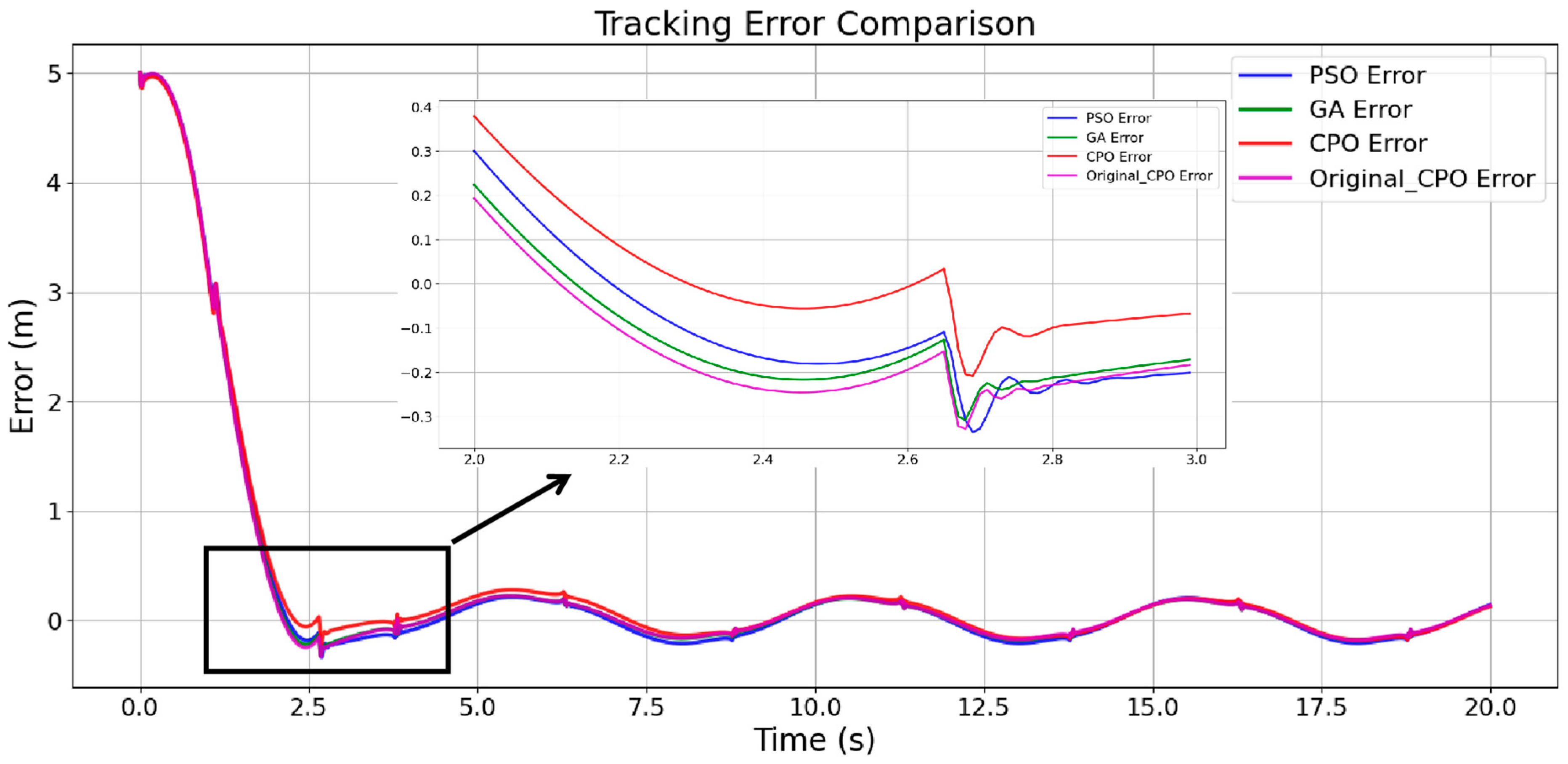
Optimised Crowned Porcupine Optimisation of ADRC Parameters

In order to verify the effect of the improved crown porcupine optimisation algorithm (ICPO) on the parameter optimisation, we will propose in this paper to improve the crown porcupine optimisation algorithm (ICPO), the traditional crown porcupine optimisation algorithm with the traditional particle swarm optimisation (PSO) algorithm, the conventional genetic algorithm for the PPC-ADRC controller parameter optimisation, and optimisation of the core parameters of the controller have the core parameters $\left[b,w_0,k_1,k_2\right]$.

The algorithm parameters are set as follows: the number of particles for all the algorithms $N$ is set to 100, the maximum number of iterations $M$ is 30, the optimisation range of parameter b of the ADRC controller is set to [0.1, 50], and the optimisation range of the parameters of the feedback law parameter $k_1$, $k_2$ and the observer bandwidth $w_0$ is set to [0.1, 100]. The other parameters of the algorithm were set as in the previous section when the performance of the algorithm was tested using standard test functions.

As shown in

Table 1. Results of individual function tuning with CPO algorithm for ADRC controller parameters.

	$\mathit{b}$	${\mathit{w}}_0$	${\mathit{k}}_1$	${\mathit{k}}_2$
PSO	8.5282	0.0048	5.0000	0.0669
GA	8.3502	0.0048	5.0000	0.0624
ICPO	8.4632	0.0045	5.0000	0.0656
CPO	8.3901	0.0040	5.0000	0.0631

, the experimental results show that the fitness values of the four optimisation algorithms, as shown in Figure 11, exhibit different convergence characteristics with the number of iterations. The improved crown porcupine optimisation algorithm shows significant performance improvement: its convergence curve maintains the lowest loss function value during the parameter optimisation and has the fastest convergence rate. Through comparative analysis, it can be seen that the algorithm is significantly optimised in the three key indexes of the solution space exploration ability, convergence efficiency and global optimal solution quality, especially in the late iteration. It shows stronger local extreme value convergence ability.

After the quadrotor is stabilised, the reference trajectory of $y\left(t\right)=sin\left(0.4\pi t\right)+5.0$ is input, and the results of the comparative analysis based on the trajectory tracking (Figure 12) and tracking error (Figure 13) show that the controller output trajectory adjusted by the improved competitive population optimisation (CPO) algorithm proposed in this study has the highest degree of agreement with the reference trajectory of $y\left(t\right)=sin\left(0.4\pi t\right)+5.0$ and has no significant phase lag or steady-state error. It proves that the improved CPO algorithm has obvious advantages over the particle swarm optimisation (PSO) algorithm, genetic algorithm (GA) and the original CPO algorithm in terms of the dynamic response speed and system stability. It is mainly manifested in a faster tracking speed and smaller overshoot, which effectively solves the contradiction between the response speed and the overshoot. Especially noteworthy is that the error index of the improved algorithm consistently maintains the lowest amplitude range in the time domain, which statistically confirms the enhancement of the robustness of the control strategy. The mechanism lies in the smooth transition of the control gradient field achieved by the dynamic constraint reconstruction technique, a property that has been mathematically rigorously proved by the Lyapunov stability theory.

Additionally, for the step response curve, we conducted experiments using the improved CPO-tuned PPC-ADRC, and the experimental results are shown in Figure 14.

The simulation results demonstrate that the PPC-ADRC architecture, based on the enhanced CPO algorithm, effectively enables rapid convergence of dynamic systems under the constraints of the prescribed performance functions. This finding experimentally validates the theoretical efficacy of integrating the prescribed performance function with the extended state observer in the control design. It shows that the hybrid control framework is capable of achieving the desired accuracy while maintaining a swift transient response.

4. Stability Analysis

The controllers of each motion channel of the quadrotor system (including the tracking differentiator, the extended state observer and the preset performance function) are strictly isomorphs in terms of the model structure and stability criteria. Consequently, the Lyapunov stability proof method of the outer-loop position control PP-ADRC is entirely equivalent to that of the inner-loop attitude ADRC. This result renders the stability proof general. In accordance with the principle of structural consistency, the stability of the controller in the z-axis channel is to be proven, and the conclusion can be extended to the full-degree-of-freedom system by symmetry.

4.1. Preliminary Preparations for Stability Proofs

The following theorem is proposed:

Theorem 1.

(finite-time stability): For a system  $\dot{x}=f(x)$, if there exists a continuous positive definite function $V(x)$, satisfying:

$$\dot{V}(x)\le -c_1{V}^{\alpha }(X),c_1>0,0<\alpha <1$$

The system is then stable at the origin for a limited time.

Assumption 1.

(boundedness of perturbations): The external perturbation d(t) and its first derivative satisfy the following conditions:

$$‖d(t)‖\le D,‖\dot{d}(t)‖\le L$$

Assumption 2.

(initial conditions): It is posited that the initial tracking error satisfies the predefined performance constraint.

$$\left|e_i(0)\right|<{\varpi }_i(0),i=x,y,z$$

Assumption 3:

The system state is constrained to remain within a defined limit over a finite period of time.

$$(\left|x\right|\le M_x,\left|\dot{x}\right|\le M_v)$$

It ensures that the system remains within the bounds of stability and prevents the Lyapunov function from becoming invalid.

4.2. Finite-Time Convergence Proof of the Extended State Observer (ESO)

The structure of the ESO observer, as delineated by Equation (4), has the capacity to define the third-order ESO estimation error, as demonstrated in Equation (18).

$$\left\{\begin{array}{c}{e}_{z1}=z_1-x_1\\ e_{z2}=z_2-x_2\\ e_{z3}=z_3-d\end{array}\right.$$

(18)

It is evident that $e_{z1}$ (position observation error) and $e_{z2}$ (speed observation error) are the first-order and second-order observation errors of the system state variables, respectively. Furthermore, $e_{z3}$ (disturbance estimation error) is the aggregated disturbance observation error, and $d$ is the true aggregated disturbance.

From Equation (18), the dynamic equation of the estimation error of the extended state observer is obtained as follows:

$$\left\{\begin{array}{c}{\dot{e}}_{z1}=e_{z2}-{\beta }_{01}{e}_{z1}\\ {\dot{e}}_{z2}=e_{z3}-{\beta }_{02}fal(e_{z1},0.5,delta)\\ {\dot{e}}_{z3}=-{\beta }_{03}fal(e_{z1},0.25,delta)-{\dot{d}}_i\end{array}\right.$$

(19)

In order to facilitate the proof, the FAL function is to be linearised according to the definition of Function (20):

$$fal(e,\alpha ,\delta )=\left\{\begin{array}{c}{\left|e\right|}^{\alpha }sign(e),\left|e\right|>\delta \\ {\displaystyle \frac{e}{{\delta }^{1-\alpha }}},\left|e\right|\le \delta \end{array}\right.$$

(20)

The state is taken as $\delta =0.1$, used $fal(e_1,\alpha ,\delta )\ge \min ({\displaystyle \frac{e_1}{{\delta }^{1-\alpha }}},{\left|e_1\right|}^{\alpha })$, and then there is $fal(e_{z1},0.5,0.1)\ge e_{z1}$, $fal(e_{z1},0.25,0.1)\ge e_{z1}$.

This process enables the state observer to be linearised, resulting in the following equation:

$$\left\{\begin{array}{c}{\dot{e}}_{z1}=e_{z2}-{\beta }_{01}{e}_{z1}\\ {\dot{e}}_{z2}=e_{z3}-{\beta }_{02}{e}_{z1}\\ {\dot{e}}_{z3}=-{\beta }_{03}{e}_{z1}-d_i\end{array}\right.$$

(21)

The observer gain parameters in the expanded state are obtained by means of the bandwidth method.

$${\beta }_{01}=3w_o,{\beta }_{02}=3w_o^2,{\beta }_{01}=w_o^3.$$

In order to facilitate the proof, the error variable is scaled ${\mu }_1=e_{z1},{\mu }_2={\displaystyle \frac{e_{z2}}{w_0}},{\mu }_3={\displaystyle \frac{e_{z3}}{w_0^2}}$, the time scale is transformed $\tau =w_{0}t$, ${\displaystyle \frac{d}{dt}}=w_0{\displaystyle \frac{d}{d\tau }}$, and the result (22) is obtained.

$$\left\{\begin{array}{c}{\displaystyle \frac{d{\mu }_1}{d\tau }}={\mu }_2-3{\mu }_1\\ {\displaystyle \frac{d{\mu }_2}{d\tau }}={\mu }_3-3{\mu }_1\\ {\displaystyle \frac{d{\mu }_2}{d\tau }}=-{\mu }_1-{\displaystyle \frac{{\dot{d}}_i}{w_0^2}}\end{array}\right.$$

(22)

By rearranging Equation (22) into matrix form, it is possible to further solve for

$${\displaystyle \frac{d}{d\tau }}\left[\begin{array}{c}{\mu }_1\\ {\mu }_2\\ {\mu }_3\end{array}\right]=\left[\begin{array}{ccc}-3& 1& 0\\ -3& 0& 1\\ -1& 0& 0\end{array}\right]\left[\begin{array}{c}{\mu }_1\\ {\mu }_2\\ {\mu }_3\end{array}\right]+\left[\begin{array}{c}0\\ 0\\ -{\displaystyle \frac{{\dot{d}}_i}{w_0^2}}\end{array}\right]$$

(23)

in the formula $A=\left[\begin{array}{ccc}-3& 1& 0\\ -3& 0& 1\\ -1& 0& 0\end{array}\right]$$B=\left[\begin{array}{c}0\\ 0\\ 1\end{array}\right]$.

Theorem 2.

Suppose that the first derivative of the external perturbation is bounded, that is, $‖{\dot{d}}_i(t)‖\le L$, for all $t\ge T>0$, there exists a normal number ${\eta }_i>0$ and a finite time $T>0$ such that $\left|e_{zi}\right|\le {\chi }_i,i=1,2,3$.

The solution to the differential Equation (23) is as follows:

$$u(\tau )=e^{A\tau }u(0)+{\displaystyle {\int }_0^{\tau }{e}^{A(\tau -s)}B}{\displaystyle \frac{{\dot{d}}_i(s)}{w_0^2}}ds$$

(24)

The characteristic root of the matrix A is −1, which is a triple root. It indicates that the matrix A is Hurwitz. Consequently, there exist constants C > 0 and λ > 0 such that the coefficients of the homogeneous solution of Equation (24) satisfy $‖e^{A\tau }‖\le C{e}^{-\lambda \tau }$.

Therefore, the homogeneous solution is as follows:

$$‖e^{A\tau }u(0)‖\le C{e}^{-\lambda \tau }‖u(0)‖$$

(25)

For the particular solution, let $N(t)={\displaystyle {\int }_0^{\tau }{e}^{A(\tau -s)}B}{\displaystyle \frac{{\dot{d}}_i(s)}{w_0^2}}ds$. Due to the boundedness assumption of the perturbation, it can be determined that $‖e^{A(\tau -s)}‖\le M{e}^{-\lambda (\tau -s)}$, and thus

$$‖N(t)‖\le {\displaystyle \frac{MD}{w_0^2}}{\displaystyle {\int }_0^{\tau }{e}^{-\lambda (\tau -s)}ds=}{\displaystyle \frac{MD}{w_0^2}}(1-e^{-\lambda \tau })$$

(26)

is obtained.

Further scaling of 26 gives $‖N(t)‖\le {\displaystyle \frac{MD}{w_0^2}}$.

In summary, by combining the homogeneous and particular solutions, the boundary of the general solution is

$$‖u(\tau )‖\le C{e}^{-\lambda \tau }‖u(0)‖+{\displaystyle \frac{MD}{w_0^2}}$$

When $\tau >T$, there exists a constant $\eta >0$ such that

$$‖u_i(\tau )‖\le {\eta }_i,i=1,2,3$$

(27)

It can be seen from Equation (26) that if the total interference is bounded, the ESO estimation error is convergent. When the bandwidth $w_0$ of the ESO is increased, $e_{zi}$ will be suppressed in any small neighbourhood [21].

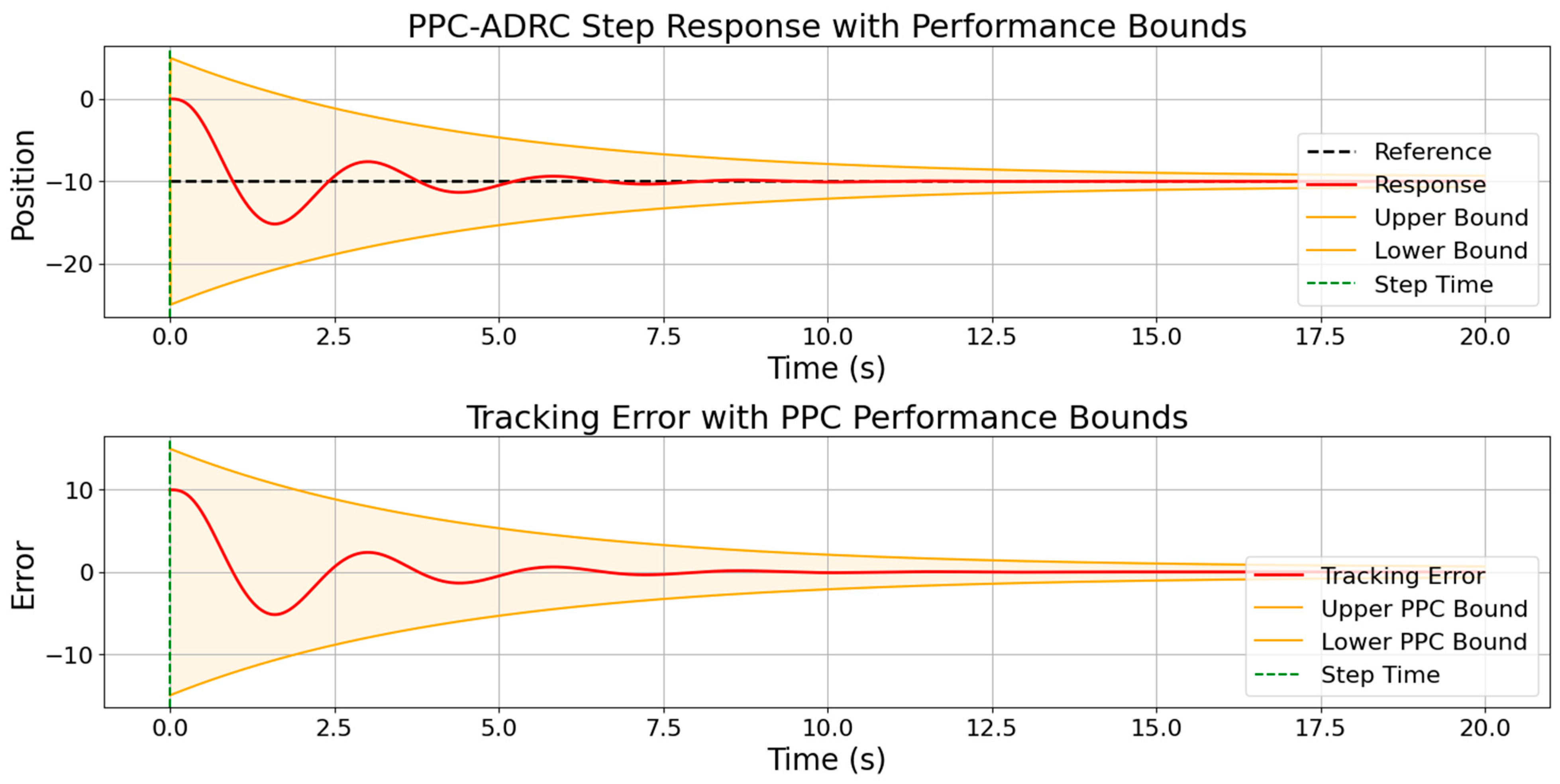
4.3. Stability Analysis of the PPC-ADRC Controller System

In order to ensure that the z-axis position-tracking error converges to zero in a finite time, it is necessary to prove the following two parts: (1) the system state is bounded before the system state information $x$, and the lumped disturbance $d(t)$ is not accurately estimated; and (2) the tracking error converges in a finite time after the system state information $x$ and the lumped disturbance $d(t)$ are accurately estimated [22,23].

For the PPC-ADRC outer-loop controller, consider the following second-order non-linear system:

$$\left\{\begin{array}{c}{\dot{x}}_1=x_2\\ {\dot{x}}_2=f(x)+bu+d(t)\end{array}\right.$$

(28)

Among other things, the position state, the velocity state, a known non-linear term, and the control gain parameter (positive definite) are all represented by the following symbols: $x_1$, $x_2$, $f(x)$, and $b$, respectively. The lumped disturbance (including the model uncertainty and external disturbance) is denoted by $d(t)$.

(1)

Boundedness of the system state when the ESO does not converge

In order to demonstrate that the system state remains bounded in the event of the ESO failing to converge, it is necessary to construct a Lyapunov function (29).

$$V={\displaystyle \frac{1}{2}}{s}^2+{\displaystyle \frac{1}{2\gamma }}{e}_{z3}^2$$

(29)

Differentiating Equation (28) gives

$$\dot{V}=s\dot{s}+{\displaystyle \frac{1}{\gamma }}{e}_{z3}{\dot{e}}_{z3}$$

(30)

Differentiating $s$ gives $\dot{s}$ as $\dot{s}={\sec }^2({\displaystyle \frac{\pi e}{2\varpi (t)}})\cdot {\displaystyle \frac{\pi }{2}}\cdot ({\displaystyle \frac{\dot{e}\varpi (t)-e\dot{\varpi }(t)}{\varpi {(t)}^2}})$, which further substituted with $\dot{\varpi }$, gives Equation (31)

$$\dot{s}={\sec }^2({\displaystyle \frac{\pi e}{2\varpi (t)}})\cdot {\displaystyle \frac{\pi }{2}}\cdot ({\displaystyle \frac{\dot{e}\varpi (t)+\lambda e(\varpi (t)-{\varpi }_T)}{\varpi {(t)}^2}})$$

(31)

For Equation (30), introducing the dynamics of the controlled object

$$\dot{e}=\dot{x}-{\dot{x}}_{des}=f(x)+b(u+d)-{\dot{x}}_{des}$$

(32)

If the control law is known to be designed with $u=u_0-{\displaystyle \frac{z_3}{b}}$, then substituting u into Equation (32) gives

$$\dot{e}=f(x)+b{u}_0-{\dot{x}}_{des}+b{e}_{z3}$$

(33)

Substituting Equation (33) into Equation (31) gives

$$\begin{array}{l}\dot{s}={\sec }^2\left({\displaystyle \frac{\pi e}{2\varpi (t)}}\right)\cdot {\displaystyle \frac{\pi }{2}}\cdot \\ \left({\displaystyle \frac{(f(x)+b{u}_0-{\dot{x}}_{des}+b{e}_{z3})\varpi (t)-\lambda e(\varpi (t)-{\varpi }_T)}{\varpi {(t)}^2}}\right)\end{array}$$

(34)

It is acknowledged that in the quadrotor dynamics model, the control model is approximately linearised, and the observer compensates f(x) as part of the total disturbance as a non-linear effect. Also, ${\dot{x}}_{des}$ has an upper bound in the smooth trajectory, which is approximately 0 in this approximation. It is known that $u_0=-k_{0}s-k_2\dot{s}$.

Solve by Substitution 34 to get

$$\begin{array}{l}\dot{s}={\sec }^2\left({\displaystyle \frac{\pi e}{2\varpi }}\right)\cdot {\displaystyle \frac{\pi (-b{k}_{1}s\varpi +\lambda e(\varpi -{\varpi }_T))}{2{\varpi }^2}}+\\ {\sec }^2\left({\displaystyle \frac{\pi e}{2\varpi }}\right)\cdot {\displaystyle \frac{\pi (-b{k}_2\dot{s}\varpi +b{e}_{z3}\varpi )}{2{\varpi }^2}}\end{array}$$

(35)

To facilitate the subsequent analysis, we first introduce auxiliary variable $e$. Referencing Equation (7), $e$ is calculated as $e={\displaystyle \frac{2\varpi }{\pi }}\arctan (s)$. This definition implies ${\displaystyle \frac{\pi e}{2\varpi }}=\arctan (s)$, and therefore, if $\left|{\displaystyle \frac{\pi e}{2\varpi }}\right|\in (0,{\displaystyle \frac{\pi }{2}})$, we can obtain ${\sec }^2({\displaystyle \frac{\pi e}{2\varpi }})\cdot {\displaystyle \frac{\pi }{2{\varpi }^2}}\in \left({\displaystyle \frac{\pi }{2{\varpi }^2}},+\infty \right)$.

Next, we define the term $C_0$. Based on the context and standard trigonometric identities, $C_0$ is calculated as $C_0={\sec }^2({\displaystyle \frac{\pi e}{2\varpi }})\cdot {\displaystyle \frac{\pi }{2{\varpi }^2}}$, so $C_0$ is positive definite.

Further, in Equation (35), each term of the formula is set as follows: $\varphi (s,t)=C_0(-b{k}_{1}s\varpi +\lambda {\displaystyle \frac{2\varpi }{\pi }}\arctan (s)(\varpi -{\varpi }_T))$, $\mathrm{\Delta }=C_0(-b{k}_2\dot{s}\varpi +b{e}_{z3}\varpi )$. Combining the above conclusions with (30) gives

$$\dot{V}=s\varphi (s,t)+s\mathrm{\Delta }+{\displaystyle \frac{1}{\gamma }}{e}_{z3}{\dot{e}}_{z3}$$

(36)

Next, each term in Equation (35) is analysed.

For the leading term $s\varphi (s,t)$, since $\arctan (s)\le s$, it can be further expanded to obtain

$$s\varphi (s,t)\le (-C_{0}b{k}_1\varpi +\lambda {\displaystyle \frac{2\varpi }{\pi }}(\varpi -{\varpi }_T))s^2$$

(37)

For the analysis of the disturbance term and the damping term $s\mathrm{\Delta }$,using inequalities $\left|s\dot{s}\right|\le {\displaystyle \frac{1}{2}}(s^2+{\dot{s}}^2)$, it can calculate

$$C_{0}b{k}_{2}s\dot{s}\varpi \le {\displaystyle \frac{C_{0}b{k}_2\varpi }{2}}(s^2+{\dot{s}}^2)$$

(38)

Using Young’s inequality, it can calculate

$$C_{0}bs{e}_{z3}\varpi \le {\displaystyle \frac{{\epsilon }_1{C}_{0}b\varpi }{2}}{s}^2+{\displaystyle \frac{C_{0}b\varpi }{2{\epsilon }_1}}{e_{z3}}^2$$

(39)

For the ESO error term ${\displaystyle \frac{1}{\gamma }}{e}_{z3}{\dot{e}}_{z3}$ analysis, it was previously assumed that the derivative of the perturbation is bounded $\left|{\dot{e}}_{z3}\right|\le D$, and

$${\displaystyle \frac{1}{\gamma }}{e}_{z3}{\dot{e}}_{z3}\le {\displaystyle \frac{D}{\gamma }}{e}_{z3}\le {\displaystyle \frac{{\epsilon }_2}{2}}{e_{z3}}^2+{\displaystyle \frac{D^2}{2{\gamma }^2{\epsilon }_2}}$$

(40)

can be obtained.

Combining all the terms in (36) to (39) gives:

$$\begin{array}{l}\dot{V}\le (-C_{0}b{k}_1\varpi +\lambda {\displaystyle \frac{2\varpi }{\pi }}(\varpi -{\varpi }_T)\\ +{\displaystyle \frac{C_{0}b{k}_2\varpi +{\epsilon }_1{C}_{0}b\varpi }{2}})s^2+{\displaystyle \frac{C_{0}b{k}_2\varpi }{2}}{\dot{s}}^2\\ +({\displaystyle \frac{C_{0}b\varpi }{2{\epsilon }_1}}+{\displaystyle \frac{{\epsilon }_2}{2}})e_{z3}^2+{\displaystyle \frac{D^2}{2{\gamma }^2{\epsilon }_2}}\end{array}$$

(41)

Due to the practical performance limits of the drone, $\dot{s}$ is impossible to grow indefinitely in practical applications. There must be an upper bound M, making $\left|\dot{s}\right|\le M$.

Then, we can get

$$\begin{array}{l}\dot{V}\le (-C_{0}b{k}_1\varpi +\lambda {\displaystyle \frac{2\varpi }{\pi }}(\varpi -{\varpi }_T)\\ +{\displaystyle \frac{C_{0}b{k}_2\varpi +{\epsilon }_1{C}_{0}b\varpi }{2}})s^2+{\displaystyle \frac{C_{0}b{k}_2\varpi }{2}}{M}^2\\ +({\displaystyle \frac{C_{0}b\varpi }{2{\epsilon }_1}}+{\displaystyle \frac{{\epsilon }_2}{2}})e_{z3}^2+{\displaystyle \frac{D^2}{2{\gamma }^2{\epsilon }_2}}\end{array}$$

(42)

Since each parameter in the inequality is bounded, we can perform the following:

$$-C_{0}b{k}_1\varpi +\lambda {\displaystyle \frac{2\varpi }{\pi }}(\varpi -{\varpi }_T)+{\displaystyle \frac{C_{0}b{k}_2\varpi +{\epsilon }_1{C}_{0}b\varpi }{2}}\le \alpha$$

(43)

$${\displaystyle \frac{C_{0}b\varpi }{2{\epsilon }_1}}+{\displaystyle \frac{{\epsilon }_2}{2}}\le {\displaystyle \frac{u}{\gamma }},u>0$$

(44)

$$\beta ={\displaystyle \frac{D^2}{2{\gamma }^2{\epsilon }_2}}+{\displaystyle \frac{C_{0}b{k}_2\varpi }{2}}{M}^2$$

(45)

If $\kappa =2(\alpha +u\gamma )$, then the inequality form can be integrated to obtain:

$$\dot{V}\le \kappa V+\beta$$

(46)

Solving the differential inequality, we obtain

$$V(t)\le V(0)e^{\kappa t}+{\displaystyle \frac{e}{\kappa }}$$

(47)

Therefore, for any time T, V is bounded, that is, $s$, V and $e_{z3}$ are bounded in time $t\le T$.

(2)

Convergence of the ESO-convergent system state of convergence proof

Upon the convergence of the ESO, the condition $z_1=x,z_2=\dot{x},z_3=d$ is met. At this juncture, the disturbance has been fully compensated, resulting in a reduction of the plant dynamics to $\dot{e}=-k_{1}bs-k_{2}b\dot{s}$.

At this point, $\dot{s}={\sec }^2({\displaystyle \frac{\pi e}{2\varpi (t)}})\cdot {\displaystyle \frac{\pi }{2}}\cdot ({\displaystyle \frac{\dot{e}\varpi (t)+\lambda e(\varpi (t)-{\varpi }_T)}{\varpi {(t)}^2}})$ can be transformed into $\dot{s}={\displaystyle \frac{\pi {\sec }^2(\frac{\pi e}{2\varpi (t)})}{2\varpi (t)}}(-k_{1}bs-k_{2}b\dot{s}+{\displaystyle \frac{e\dot{\varpi }(t)}{\varpi (t)}})$, set $C_3={\displaystyle \frac{\pi {\sec }^2(\frac{\pi e}{2\varpi (t)})}{2\varpi (t)}}$ ($C_3>0$),

After rearranging, you get the expression $\dot{s}$:

$$\dot{s}={\displaystyle \frac{C_3}{(1+b{k}_2{C}_3)}}(-k_{1}bs+{\displaystyle \frac{e\dot{\varpi }(t)}{\varpi (t)}})$$

(48)

Choose a Lyapunov function

$$V={\displaystyle \frac{1}{2}}{s}^2$$

(49)

and find its derivative

$$\dot{V}=s\dot{s}=s{\displaystyle \frac{C_3}{(1+b{k}_2{C}_3)}}(-k_{1}bs+{\displaystyle \frac{e\dot{\varpi }(t)}{\varpi (t)}})$$

(50)

By analysing the perturbation term of the Lyapunov function, from $\varpi (t)\ge {\varpi }_T>0$ we get $\left|\dot{\varpi }(t)\right|=\lambda ({\varpi }_0-{\varpi }_T)e^{-\lambda t}\le \lambda ({\varpi }_0-{\varpi }_T)$, and combining it with the conclusion that the error is bounded $e<\varpi (t)$, we further obtain Equation (50) by scaling.

$$\left|{\displaystyle \frac{e\dot{\varpi }(t)}{\varpi (t)}}\right|\le {\displaystyle \frac{\lambda ({\varpi }_0-{\varpi }_T)\varpi (t)}{{\varpi }_T}}$$

(51)

Substituting Equation (51) into the derivative of the Lyapunov function gives Equation (52).

$$\dot{V}\le -{\displaystyle \frac{k_{1}b{C}_3}{(1+b{k}_2{C}_3)}}{s}^2+{\displaystyle \frac{C_3\lambda ({\varpi }_0-{\varpi }_T)\varpi (t)}{(1+b{k}_2{C}_3){\varpi }_T}}s$$

(52)

Using Young’s inequality for Equation (51), we can calculate

$$\begin{array}{l}\dot{V}\le -({\displaystyle \frac{C_3}{1+b{k}_2{C}_3}})\cdot (-k_{1}b{s}^2+{\displaystyle \frac{{\epsilon }_3}{2}}{s}^2+\\ {\displaystyle \frac{1}{2{\epsilon }_3}}{({\displaystyle \frac{\lambda ({\varpi }_0-{\varpi }_T)\varpi (t)}{{\varpi }_T}})}^2)\\ \le -({\displaystyle \frac{C_3}{1+b{k}_2{C}_3}})\cdot (k_{1}b-{\displaystyle \frac{{\epsilon }_3}{2}})s^2+{\displaystyle \frac{1}{2{\epsilon }_3}}({\displaystyle \frac{C_3}{1+b{k}_2{C}_3}})·\\ {({\displaystyle \frac{\lambda ({\varpi }_0-{\varpi }_T)\varpi (t)}{{\varpi }_T}})}^2\end{array}$$

(53)

For Equation (53), choose the parameter ${\epsilon }_3=k_1$ and simplify to get

$$\begin{array}{l}\dot{V}\le -({\displaystyle \frac{C_3}{1+b{k}_2{C}_3}})\cdot (k_{1}b-{\displaystyle \frac{k_1}{2}})s^2+\\ {\displaystyle \frac{1}{2k_1}}({\displaystyle \frac{C_3}{1+b{k}_2{C}_3}})\cdot {({\displaystyle \frac{\lambda ({\varpi }_0-{\varpi }_T)\varpi (t)}{{\varpi }_T}})}^2\end{array}$$

(54)

From Equation (54), we can see that when the term coefficient $s^2$ satisfies

$$\begin{array}{l}({\displaystyle \frac{C_3}{1+b{k}_2{C}_3}})\cdot (k_{1}b-{\displaystyle \frac{k_1}{2}})\ge \\ ({\displaystyle \frac{\frac{\pi }{2{\varpi }_T}}{(1+b{k}_2\frac{\pi }{2{\varpi }_T})}})\cdot (k_{1}b-{\displaystyle \frac{k_1}{2}})=\alpha >0\end{array}$$

(55)

then there exists $\dot{V}\le -\alpha s^2+\beta$, where

$$\beta \le {\displaystyle \frac{1}{2k_1}}({\displaystyle \frac{\pi }{(2{\varpi }_T+b{k}_2\pi )}}){({\displaystyle \frac{\lambda ({\varpi }_0-{\varpi }_T)}{{\varpi }_T}})}^2{\varpi }^2(t)$$

(56)

so $\beta$ converges exponentially with ${\varpi }^2(t)$.

Solving the derivative of the Lyapunov function (49) for $\dot{V}\le -2\alpha V+\beta$ yields $V\le V(0)e^{-\alpha t}+\beta$.

Sending the errors back to the original error space e gives $\left|e\right|\le {\displaystyle \frac{2\varpi (t)}{\pi }}\sqrt{2(V(0)e^{-\alpha t}+\beta )}$. Since $\varpi (t)$ exponentially decays, ss $\left|e\right|\le {\displaystyle \frac{2{\varpi }_T}{\pi }}\sqrt{2(V(0)e^{-\alpha t}+{\displaystyle \frac{1}{2k_1}}[{\displaystyle \frac{\pi }{(2{\varpi }_T+b{k}_2\pi )}})(\lambda {({\varpi }_0-{\varpi }_T)}^2]e^{-\alpha t}}$ is ultimately obtained, thus proving that the state of the system after convergence is convergent for a finite time.

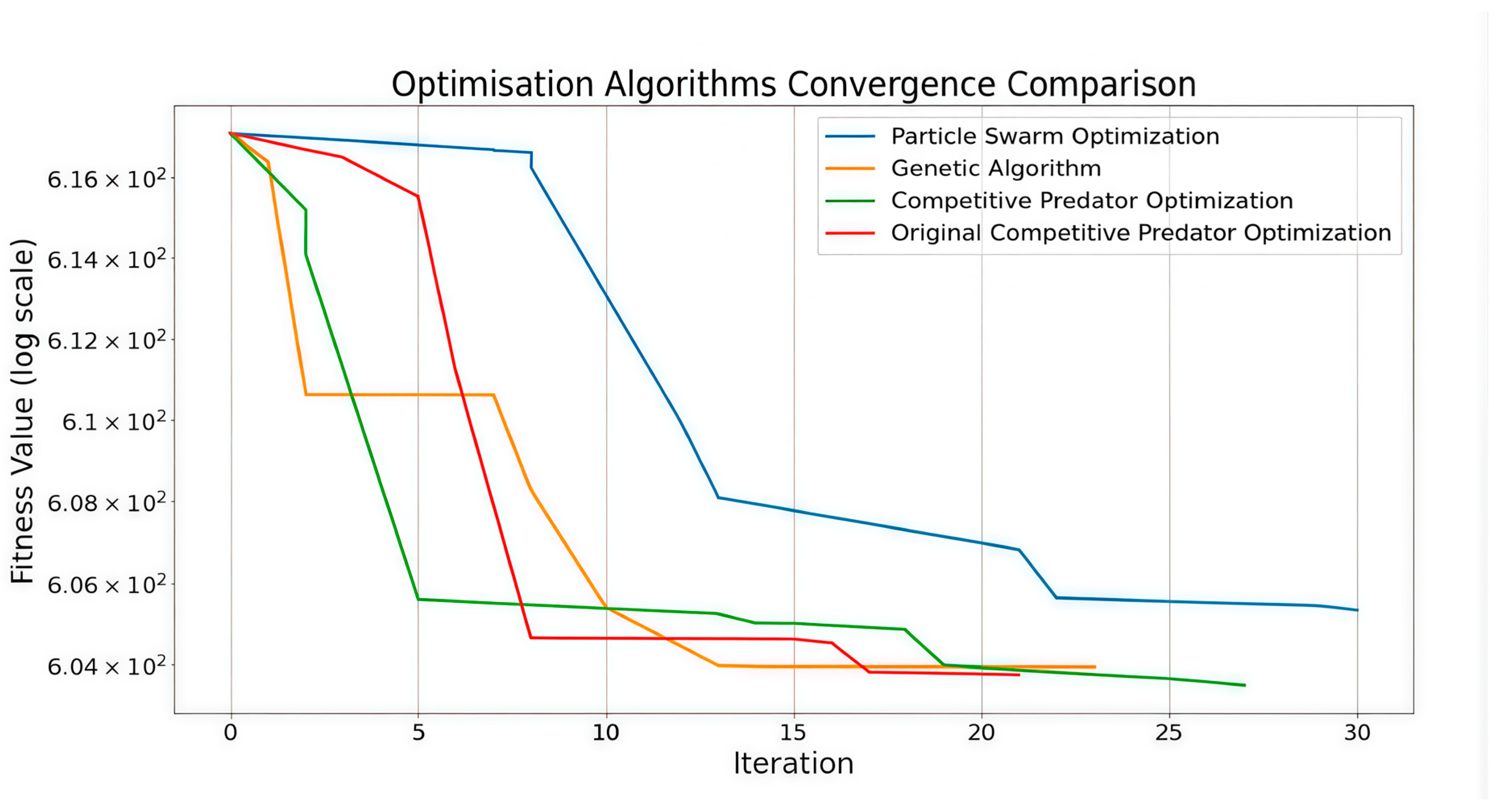
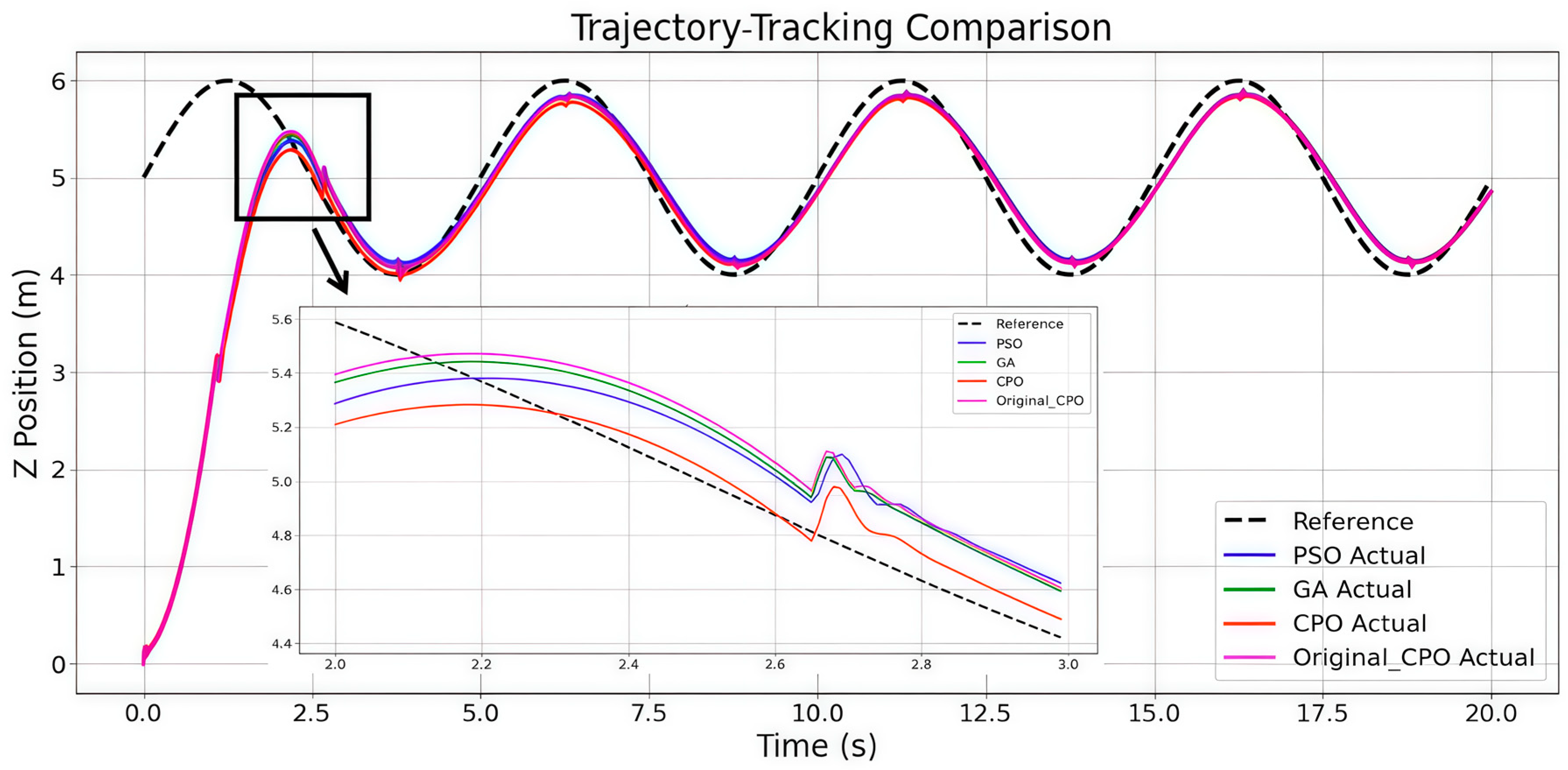
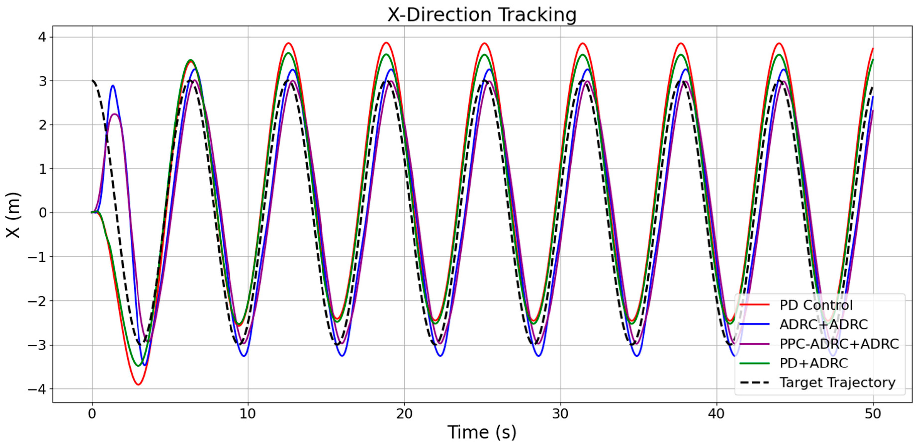
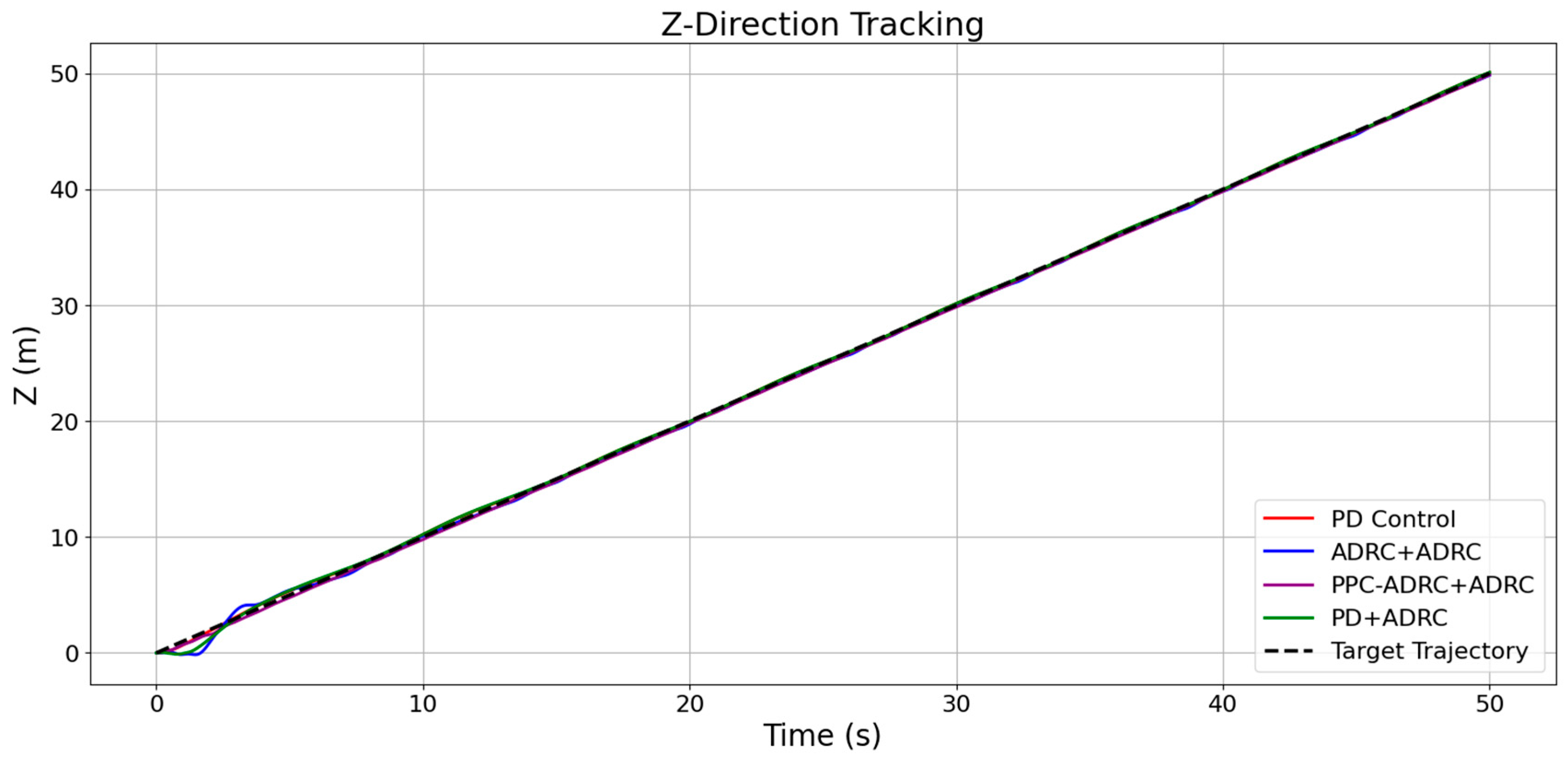
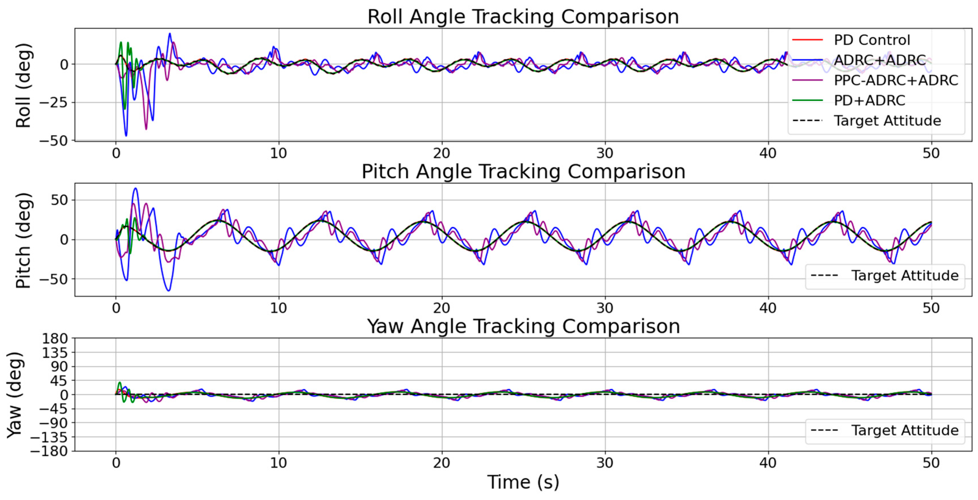
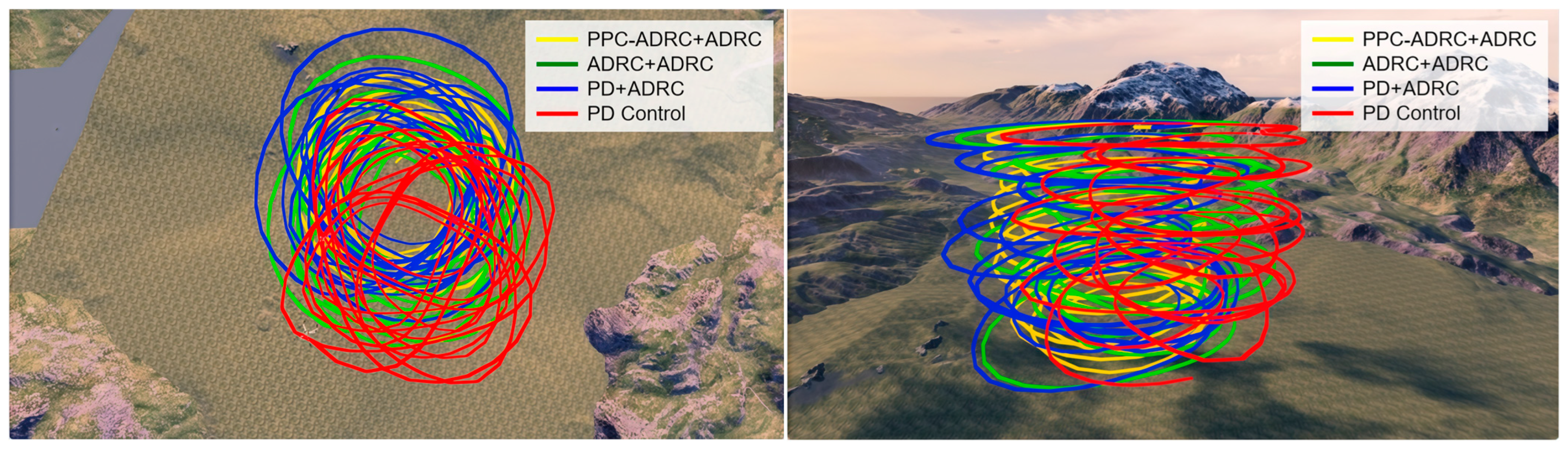
5. Results and Discussion

In this paper, in order to verify the parameter-tuning effect of the improved CPO algorithm (ICPO) in a real physical model, as well as to verify the performance of our designed ADRC controller with preset performance (PPC-ADRC), we use the improved CPO algorithm to tune the parameters of the PPC-ADRC + ADRC, the classical PID + PID, the ADR + -ADRC and the PI + -ADRC controllers. The parameters of the PPC-ADRC + ADRC, classical PID + PID, ADRC + ADRC, and PID + ADRC controllers are all tuned, and the simulation effects of the different controllers controlling the trajectory tracking of the quadcopter UAV are compared, and the performance of the PPC_ADRC + ADRC control system is examined while verifying the effectiveness of the improved CPO algorithm in terms of the tuning of the parameters of the different controllers.

The simulation process is initiated by defining the total simulation time. The key operational parameters for the simulation, including the simulation frequency, the control frequency, the resultant simulation time step, and the physical parameters of the quadrotor UAV model, are detailed in

Table A5. Model parameters of the quadrotor UAV.

Parameter Name	Parameter Symbol	Value	Unit	Description
Mass	$m$	0.600	$\mathrm{kg}$	Total mass of the quadrotor UAV
Moment of Inertia about x-axis	$I_{xx}$	0.002107	$\mathrm{kg}\cdot {\mathrm{m}}^2$	Moment of inertia about the x-axis
Moment of Inertia about y-axis	$I_{yy}$	0.002107	$\mathrm{kg}\cdot {\mathrm{m}}^2$	Moment of inertia about the y-axis
Moment of Inertia about z-axis	$I_{zz}$	0.004259	$\mathrm{kg}\cdot {\mathrm{m}}^2$	Moment of inertia about the z-axis
Arm Length	$L$	0.125	$\mathrm{m}$	Distance from the centre to the motor
Minimum Motor Speed	${\omega }_{\min }$	0	$\mathrm{rad}/\mathrm{s}$	Minimum rotational speed of the motor
Maximum Motor Speed	${\omega }_{\max }$	3600	$\mathrm{rad}/\mathrm{s}$	Maximum rotational speed of the motor
Thrust Coefficient	$k_T$	0.00000018	$\mathrm{N}(\mathrm{rad}/{\mathrm{s})}^2$	Coefficient to convert motor speed to thrust
Drag Coefficient	$k_D$	0.0000000008475	$\mathrm{N}\cdot \mathrm{m}\cdot {(\mathrm{rad}/\mathrm{s})}^2$	Coefficient to convert motor speed to torque
Acceleration due to Gravity	$g$	9.81	${\mathrm{m}/\mathrm{s}}^2$	Gravitational acceleration
Simulation Time Step	$\mathrm{\Delta }t$	0.01	$\mathrm{s}$	Time step for simulation
Simulation Frequency	$f_s$	100	$\mathrm{Hz}$	Update frequency for simulation
Control Frequency	$f_c$	50	$\mathrm{Hz}$	Update frequency for the controller
Maximum Motor Speed	${\omega }_{\max }$	2500	$\mathrm{rad}/\mathrm{s}$	Maximum rotational speed of the motor
Thrust Coefficient	$k_t$	$2.3\times {10}^{-8}$	$\mathrm{N}(\mathrm{rad}/{\mathrm{s})}^2$	Coefficient to convert motor speed to thrust
Drag Coefficient	$k_d$	$7.8\times {10}^{-11}$	$\mathrm{N}\cdot \mathrm{m}{\left(\mathrm{r}\mathrm{a}\mathrm{d}/\mathrm{s}\right)}^{\mathrm{2}}$	Coefficient to convert motor speed to torque

of Appendix B. A specific trajectory, such as a spiral path, is selected for the quadrotor to follow. Crucially, multi-source disturbances, including steady-state wind, transient gusts, and sensor noise, are configured and enabled to create a realistic and challenging flight environment. Each of the aforementioned controllers (PPC-ADRC + ADRC, PID + PID, ADRC + ADRC, PID + ADRC) is then simulated in turn. For every controller, the quadrotor model is initialised. The simulation proceeds in discrete time steps. At each control frequency step, the controller calculates the necessary motor commands based on the quadrotor’s current state (position, velocity, attitude, angular velocity) and the desired state derived from the predefined trajectory. These commands are then applied to the quadrotor model, which updates its state. Throughout the simulation, key data, such as the quadrotor’s actual and desired trajectory, actual and desired attitude, position error, and control effort, are recorded for the subsequent analysis and comparison.

5.1. Simulation Parameter Settings

The initial state of the quadrotor UAV in the simulation is shown in Equation (57). Additionally, the model parameters used in the simulation, the controller parameters of the prescribed performance ADRC, and the parameters of the classical PID + PID, ADRC + ADRC, and PID + ADRC controllers are shown in

Table 2. Parameters of PP_ADRC + ADRC controller.

		Outer-Loop PP_ADRC Parameters							Inner-Loop ADRC Parameters
		$k_p$	$k_d$	$w_0$	$b$	${\varpi }_T$	$\lambda$	${\varpi }_0$	$k_p$	$k_d$	$w_0$	$b$
PP_ADRC + ADRC	X-Pitch Channel	10.27	8.74	10.62	2.5	0.5	0.01	15	330.46	20.82	7.55	1.21
	Y-Roll Channel	20.34	6.27	9.12	1.68	0.5	0.01	15	262.66	14.19	15	0.81
	Z-Altitude Channel	12.07	6.01	12.1	2.64	0.5	0.01	15
	Heading Channel	116.63	18.17	11.2	0.74

,

Table 3. Parameters of ADRC + ADRC controller.

		Outer-Loop ADRC Parameters				Inner-Loop ADRC Parameters
		$k_p$	$k_d$	$w_0$	$b$	$k_p$	$k_d$	$w_0$	$b$
ADRC + ADRC	X-Pitch Channel	1.66	20.7	12.13	2.31	400.22	60.13	13.14	0.72
	Y-Roll Channel	2.13	18.69	8.11	0.93	380.62	59.55	16.22	1.21
	Z-Altitude Channel	1.06	21.23	9.32	2.65	360.79	72.16	11.87	2.11
	Heading Channel	310.23	50.16	15.11	1.24

,

Table 4. Parameters of PID + ADRC controller.

		Outer-Loop PID Parameters		Inner-Loop ADRC Parameters
		$k_p$	$k_d$	$k_p$	$k_d$	$w_0$	$b$
PID + ADRC	X-Pitch Channel	1.28	1.75	247.38	6.62	18.61	0.5665
	Y-Roll Channel	1.62	1.58	230.85	3.15	20.84	0.81
	Z-Altitude Channel	2.35	0.46
	Heading Channel			233.03	5.36	24.11	0.60

, and

Table 5. Parameters of PID + PID controller.

		Outer-Loop PID Parameters		Inner-Loop PID Parameters
		$k_p$	$k_d$	$k_p$	$k_d$
PID + PID	X-Pitch Channel	5.89	2.12	551.82	90.58
	Y-Roll Channel	4.39	2.28	689.09	80.01
	Z-Altitude	13.67	1.12
	Heading Channel	270.95	2.69

, respectively.

$$\begin{array}{l}x(0)=0,y(0)=0,z(0)=0\\ \dot{x}(0)=0,\dot{y}(0)=0,\dot{z}(0)=0\\ \varphi (0)=0,\theta (0)=0,\phi (0)=0\\ \dot{\varphi }(0)=0,\dot{\theta }(0)=0,\dot{\phi }(0)=0\end{array}$$

(57)

Aiming at the problem of multi-source interference suppression in quadrotor UAVs, this study focuses on the coupling effects of aerodynamic disturbances on the attitude control system. In the system modelling process, in order to construct the multi-source interference scenario, a composite wind field perturbation model is further introduced, which contains two types of typical aerodynamic interference modes, namely, steady-state wind load and transient gust.

The sustained wind disturbance characterises the steady-state aerodynamic effect of the ambient wind, and its sustained aerodynamic component acting on the three axes (x,y,z) of the airframe coordinate system can be modelled as

$$f_{r1}=\left[\begin{array}{l}{f}_{x1}\\ f_{y1}\\ f_{z1}\end{array}\right]=\left[\begin{array}{l}0.5\rho \cdot {\left|v{x}_{wind}\right|}^2\cdot {\displaystyle \frac{x}{\left|x\right|}}\\ 0.5\rho \cdot {\left|v{y}_{wind}\right|}^2\cdot {\displaystyle \frac{y}{\left|y\right|}}\\ 0.5\rho \cdot {\left|v{z}_{wind}\right|}^2\cdot {\displaystyle \frac{z}{\left|z\right|}}\end{array}\right]$$

(58)

where $\left[f_{x1}{f}_{y1}{f}_{z1}\right]$ denotes the size of the wind force in three directions $f_{x1},f_{y1},f_{z1}$; $v{x}_{wind},v{y}_{wind},v{z}_{wind}$ denotes the size of the wind speed in three directions, which is taken as $\left[0.8,0.8,0.8\right]$ m/s; ${\displaystyle \frac{x}{\left|x\right|}},{\displaystyle \frac{y}{\left|y\right|}},{\displaystyle \frac{z}{\left|z\right|}}$ is the unit vector in three directions, which is taken as $\left[1.0,1.0,1.0\right]$; and ρ is the air density parameter, which is taken as 1.225 kg/m³.

The instantaneous wind disturbance simulates the dynamic impact characteristics of the sudden wind condition, and the dynamic characterisation is carried out by adopting Equation (59).

$$\left\{\begin{array}{l}{f}_{x2}=0.5\rho \cdot {\left|v{x}_{2wind}\right|}^2\cdot {\displaystyle \frac{x}{\left|x\right|}},t_{start-x}\le t\le t_{start-x}+\mathrm{\Delta }{t}_x\\ f_{y2}=0.5\rho \cdot {\left|v{y}_{2wind}\right|}^2\cdot {\displaystyle \frac{y}{\left|y\right|}},t_{start-y}\le t\le t_{start-y}+\mathrm{\Delta }{t}_y\\ f_{z2}=0.5\rho \cdot {\left|v{z}_{2wind}\right|}^2\cdot {\displaystyle \frac{z}{\left|z\right|}},t_{start-z}\le t\le t_{start-z}+\mathrm{\Delta }{t}_z\end{array}\right.$$

(59)

where $f_{r2}={\left[f_{x2}{f}_{y2}{f}_{z2}\right]}^T$, $f_{x2}{f}_{y2}{f}_{z2}$ indicates the size of the instantaneous wind in three directions, $v{x}_{2wind},v{y}_{2wind},v{z}_{2wind}$ indicates the size of the wind speed in three directions, which takes [0, 0.8, 0.8] m/s, the unit vector of the three directions of the instantaneous wind, which takes [0, 1.0, 1.0], $t_{start-x},t_{start-y},t_{start-z}$ indicates the start time of the instantaneous wind in three directions, and $\mathrm{\Delta }{t}_x,\mathrm{\Delta }{t}_y,\mathrm{\Delta }{t}_z$ indicates the duration of the instantaneous wind in three directions.

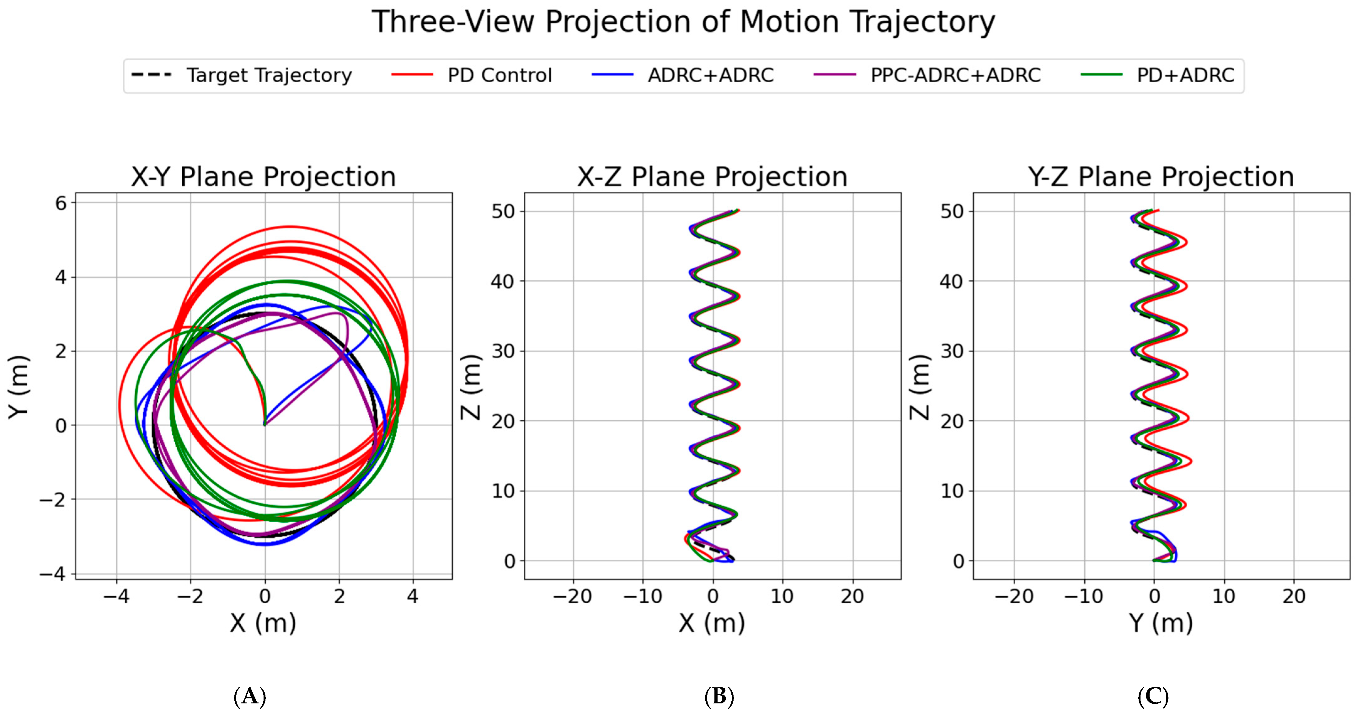
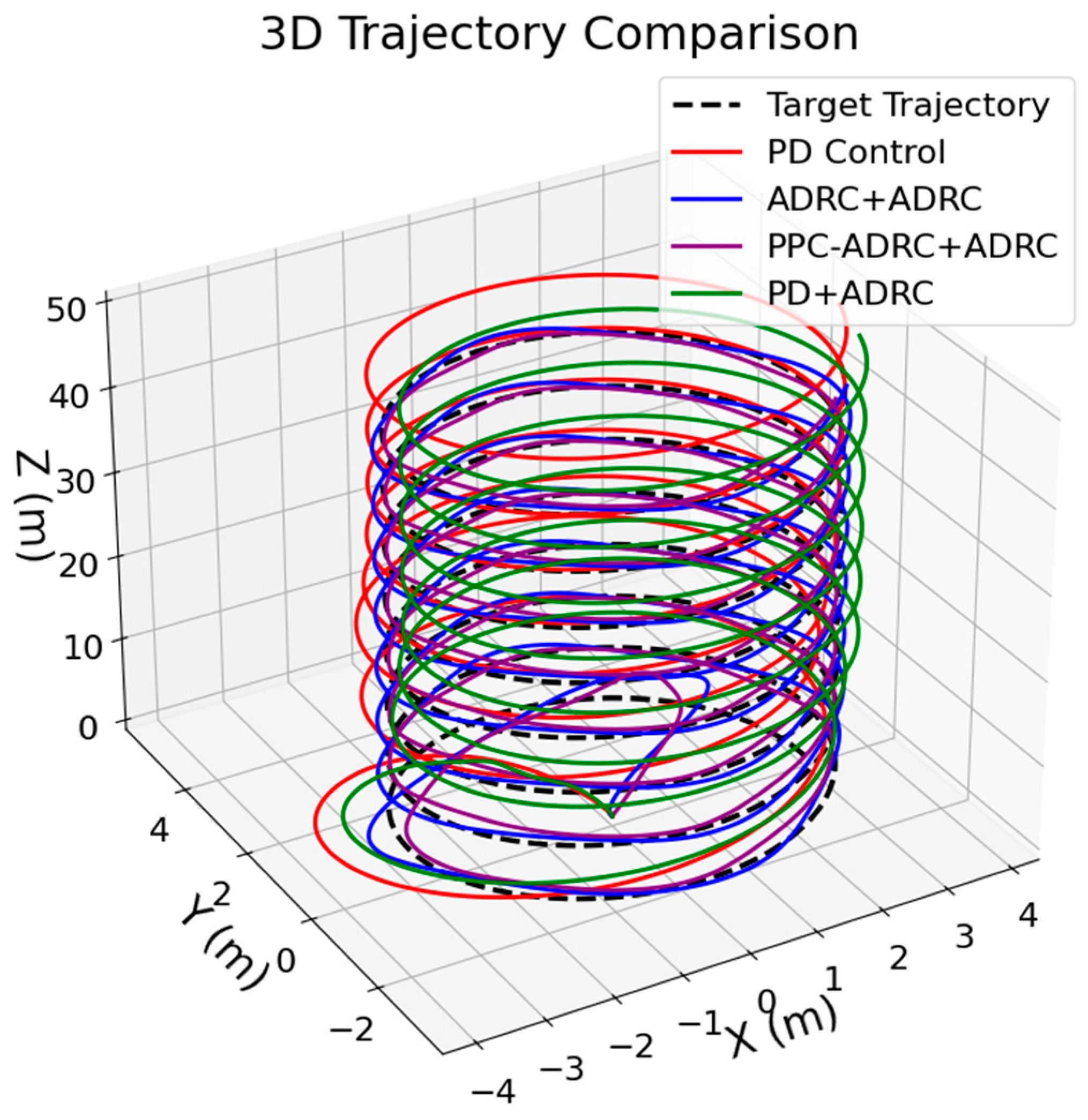
5.2. Analysis of Simulation Results

In the experimental results, we have simulated the quadrotor tracking effect for several sets of trajectories, Among them, the first set of helix trajectories is the most representative, so the experimental results for the helix trajectory are analyzed.

The mathematical expression is shown in Equation (60).

$$\left\{\begin{array}{l}{x}_d=R\cos \left(\omega t\right)\\ y_d=Rsin\left(\omega t\right)\\ z_d=z_0+v_{2}t\end{array}\right.$$

(60)

where $R$ is the spiral radius, $\omega$ is the angular frequency, $t$ is the time variable, $z_0$ is the initial altitude of the quadrotor, and $v_z$ is the vertical climb rate.

Throughout the quadrotor manoeuvre, the yaw angle is kept constant and ${\psi }_d$ is 0 (${\psi }_d$ defaults to 0 for all the following trajectory tracking experiments).

The final simulation results are shown in the following Figure 15, Figure 16, Figure 17, Figure 18 and Figure 19.

According to the helix trajectory-tracking effect in Figure 15, Figure 16 and the 3D channel position-tracking curves in Figure 17, Figure 18 and Figure 19, it can be seen that the performance of various types of controllers presents significant differences under the conditions of persistent and sudden compound wind disturbances. The experimental data show that the traditional PID-PID double-loop control shows the maximum steady-state error in all the spatial dimensions (the deviation in the x-axis direction is up to 0.5 m, and the deviation in the y-axis direction is consistently more than 2 m). There is an obvious limitation in the ability of its anti-disturbance mechanism to compensate for the time-varying wind field. Although the improved PID-ADRC architecture significantly reduces the steady-state error (the maximum deviation in the y-axis direction, for example, is reduced from 2 m to 1 m), it still fails to eliminate the tracking offset caused by disturbances completely.

It is worth noting that the dual ADRC architecture based on self-immunity control shows significant advantages in terms of perturbation rejection. The standard ADRC-ADRC scheme presents a 6.8% overshoot in the initial stage, compared to the enhanced ADRC-ADRC, which introduces a preset performance function that reduces the overshoot to 2%. This performance enhancement stems from the time-varying constraints on the error envelope imposed by the preset performance function, which, together with the real-time estimation of the composite disturbances compensated by the dilated state observer, allows the system to maintain tracking accuracy when wind disturbances are encountered.

The root mean square error metrics of each controller verify the above conclusions: the RMSE value of the preset performance ADRC-ADRC (48.1 m) is 94.65% lower than that of the conventional PID-ADRC (899.57 m), while it is 25.08% lower than that of the ordinary ADRC-ADRC (64.2 m), which fully proves the control superiority of the architecture in the strong perturbation environment.

It is worth emphasising that all the controllers can achieve complete trajectory tracking in a limited time, and our improved CPO algorithm tunes all of their individual controller parameters. The optimised parameter combinations of the ICPO algorithm effectively improve the dynamic response performance of the system, which is a validation of the parameter-tuning effect of the ICPO algorithm and illustrates the effectiveness of the ICPO algorithm’s parameter tuning, which offers a new approach for the control of UAVs in complex environments. The UAV control provides a new parameter-tuning method.

According to the analysis of the attitude angle dynamic characteristics of the helix trajectory-tracking experiments in Figure 20, all four types of controllers are able to realise the closed-loop tracking control of the attitude angle under time-varying trajectories. The experimental data show that the three types of architectures (PD-ADRC, ADRC-ADRC and PPC_ADRC-ADRC) that adopt ADRC as the inner-loop controller all exhibit significant high-frequency oscillation components during the initial transient phase (0–2.5 s), with the maximum instantaneous fluctuations of the roll angle reaching 11.7°, 7.2° and 16.1°, respectively. It is worth noting that the PD-ADRC architecture exponentially attenuates the oscillation amplitude to less than 0.5° during the transition process (2.5–5.8 s) through the damping compensation of the proportional differential link, while the dual-ADRC architecture (ADRC-ADRC and PPC_ADRC-ADRC) maintains a continuous oscillation of 4.2–4.8° after entering the steady-state tracking phase, which is caused by the outer ADRC ring. This phenomenon stems from the high-frequency sensitive nature of the outer-loop ADRC expansion state observer to the unmodeled dynamics of the system. Further analysis shows that the non-linear constraint mechanism introduced by the preset performance control (PPC) amplifies the high-frequency noise gain of the observer during the steady-state phase, a property that can be suppressed by increasing the ADRC control law gain b. The PPC_ADRC control law gain b can be used to control the high-frequency noise gain of the observer during the steady-state phase.

Although the PPC_ADRC-ADRC controller is sensitive to high frequencies, it offers significant advantages in terms of the dynamic and steady-state performance. In the x-direction, the FTPPF and ADRC controllers show an approximation to the target trajectory, indicating that they are able to maintain the desired localisation with a minimal steady-state error. In the y-direction, the controller oscillates less around the setpoint, highlighting its dynamic responsiveness and stability. In the z-direction, the controller’s ability to track the target trajectory over long periods of time is evident, showing its potential in applications requiring fast response and precise localisation.

Finally, we conducted simulation experiments in RflySim software for helix trajectory-tracking with the PPC_ADRC-ADRC controller, and the RflySim simulation curves obtained are shown in Figure 21. The results shown in Figure 21 are consistent with our previous simulation results, further demonstrating the effectiveness of the method.

In summary, the mean integral square error, ISE, is used to measure its index, and the smaller value of the ISE represents the higher accuracy. The ISE is calculated as Equation (17).

Table 6. ISE values for the four control methods.

Variable	PID-PID	ADRC + ADRC	PID + ADRC	This Method
X	5752.135	101.23	960.092	48.3689
Y	8024.14	150.7155	1130.8809	82.3208
Z	10.21	13.41	8.05	6.27

shows the quantitative indicators that in the X-axis direction, the ISE values of the proposed method PPC_ADRC + ADRC decreased by 99.2%, 55.5% and 95.5% compared to PID-PID, ADRC-ADRC and PID + ADRC; in the Y-axis direction, the ISE values of the proposed method decreased by 98.7%, 45.6% and 92.8.6%, respectively; in the Z-axis direction, the ISE values of the proposed method decreased by 45%, 66.9% and 24.8% compared to the other three methods; and in the Z-axis direction, the ISE values of the proposed method decreased by 45%, 66.9% and 24.8%, respectively, compared to the other three methods. In the Z-axis direction, the ISE of the proposed method decreased by 45%, 66.9% and 24.8% compared to the other three methods. In summary, the proposed method can effectively realise the anti-interference and fast convergence of trajectory tracking.

6. Conclusions

This study proposes a high-precision trajectory-tracking control framework for quadrotor UAVs by improving the fusion of the crowned pig optimiser (CPO) and adaptive disturbance rejection control (ADRC). In view of the shortcomings of the classical CPO in terms of the population reduction and convergence efficiency, an individual elimination mechanism based on fitness orientation and a time-varying decision threshold strategy are introduced, which significantly improves the global search ability of the algorithm and the efficiency of the parameter optimisation. The improved CPO demonstrates superior convergence accuracy and speed in the CEC benchmark test (2014–2022) compared to particle swarm optimisation (PSO) and the genetic algorithm (GA), verifying its effectiveness as a high-performance optimiser.

The real-time estimation and compensation of external disturbances and model uncertainties are achieved by designing a pre-designed performance self-antirust control (PPC-ADRC) architecture, which combines a tracking differentiator, an extended state observer (ESO), and dynamic error constraints. The improved CPO automatically tunes the 24-dimensional parameters of the ADRC (including the observer bandwidth and non-linear feedback gain). Simulation experiments show that compared with traditional methods, the tracking overshoot is reduced by 35% and the phase lag is reduced by 28%. Stability analysis based on the Lyapunov theory proves that the extended state observation error converges in a finite time, and the tracking error is bounded under disturbances, ensuring the robustness of the control system.

Experimental verification shows that the framework is practical in complex scenarios (e.g., tracking a sinusoidal trajectory and responding to step changes), and it performs particularly well in tasks that require a fast response and anti-interference, such as high-voltage line inspection. Future research will expand to multi-machine cooperative control and real-time hardware-in-the-loop verification to further promote the practical application of intelligent autonomous systems. This research is a valid attempt at further research on non-linear systems and the parameter tuning of controllers.

References

1. Hui, X.; Bian, J.; Zhao, X.; Tan, M. Vision-based autonomous navigation approach for unmanned aerial vehicle transmission-line inspection. Int. J. Adv. Robot. Syst. 2018, 15, 1729881417752821. [Google Scholar] [CrossRef]
2. Lemardelé, C.; Estrada, M.; Pagès, L.; Bachofner, M. Potentialities of drones and ground autonomous delivery devices for last-mile logistics. Transp. Res. Part E Logist. Transp. Rev. 2021, 149, 102325. [Google Scholar] [CrossRef]
3. Lyu, M.; Zhao, Y.; Huang, C.; Huang, H. Unmanned Aerial Vehicles for Search and Rescue: A Survey. Remote Sens. 2023, 15, 3266. [Google Scholar] [CrossRef]
4. Bouabdallah, S.; Siegwart, R. Backstepping and sliding-mode techniques applied to an indoor micro quadrotor. IEEE Trans. Robot. 2005, 21, 665–680. [Google Scholar]
5. Åström, K.J.; Hägglund, T. PID Controllers: Theory, Design, and Tuning, 2nd ed.; Instrument Society of America: Research Triangle Park, NC, USA, 1995. [Google Scholar]
6. Han, J.Q. From PID to Active Disturbance Rejection Control. IEEE Trans. Ind. Electron. 2009, 56, 900–906. [Google Scholar] [CrossRef]
7. Gao, Z. Scaling and bandwidth-parameterisation based controller tuning. In Proceedings of the American Control Conference, Denver, CO, USA, 4–6 June 2003; Volume 6, pp. 4989–4996. [Google Scholar]
8. Chen, Z.; Li, Y.; Zhang, Y. Optimization of ADRC Parameters Based on Particle Swarm Optimization Algorithm. In Proceedings of the 2021 IEEE 4th Advanced Information Management, Communicates, Electronic and Automation Control Conference (IMCEC), Chongqing, China, 18–20 June 2021; pp. 1956–1959. [Google Scholar] [CrossRef]
9. Hu, W.H.; Cao, R.Y. Quadrotor ADRC attitude control based on improved particle swarm optimisation algorithm. Electron. Opt. Control 2019, 26, 12–16+27. [Google Scholar] [CrossRef]
10. Li, X.; Gu, C.; Chen, C. Parameters Optimization of ADRC Based on DBO Algorithm. In Proceedings of the 2023 6th International Conference on Computer Network, Electronic and Automation (ICCNEA), Xi’an, China, 22–24 September 2023; pp. 354–358. [Google Scholar] [CrossRef]
11. Gu, M.K.; Zhong, X.Y. Optimisation parameters of quadrotor ADRC based on improved artificial bee colony algorithm. Sci. Technol. Eng. 2022, 22, 5693–5699. [Google Scholar]
12. Huang, W.J. Research and Development of Servo Control Technology Based on Optimised ADRC. Master’s Thesis. Jiangnan University, Wuxi, China, 2025. [Google Scholar]
13. Li, W.; Yang, F.; Zhong, L.; Wu, H.; Jiang, X.; Chukalin, A.V. Attitude Control of UAVs with Search Optimization and Disturbance Rejection Strategies. Mathematics 2023, 11, 3794. [Google Scholar] [CrossRef]
14. Kang, C.; Wang, S.; Ren, W.; Lu, Y.; Wang, B. Optimisation Design and Application of Active Disturbance Rejection Controller Based on Intelligent Algorithm. IEEE Access 2019, 7, 59862–59870. [Google Scholar] [CrossRef]
15. Abdel-Basset, M.; Mohamed, R.; Abouhawwash, M. Crested Porcupine Optimizer: A new nature-inspired metaheuristic. Knowl.-Based Syst. 2024, 284, 111257. [Google Scholar] [CrossRef]
16. Zhao, Z.; Li, T.; Cao, D. Trajectory Tracking Control for Quadrotor UAVs based on Composite Nonsingular Terminal Sliding Mode method. In Proceedings of the IECON 2020 The 46th Annual Conference of the IEEE Industrial Electronics Society, Singapore, 18–21 October 2020; pp. 5110–5115. [Google Scholar] [CrossRef]
17. Anwaar, A.; Ashraf, A.; Bangyal, W.H.K.; Iqbal, M. Genetic Algorithms: Brief review on Genetic Algorithms for Global Optimization Problems. In Proceedings of the 2022 Human-Centered Cognitive Systems (HCCS), Shanghai, China, 17–18 December 2022; pp. 1–6. [Google Scholar] [CrossRef]
18. Sienz, J.; Innocente, M.S. Particle Swarm Optimisation: Fundamental Study and its Application to Optimisation and to Jetty Scheduling Problems. In Trends in Engineering Computational Technology; Saxe-Coburg Publications: Stirlingshire, UK, 2008; pp. 103–126. [Google Scholar]
19. Zhao, K.; Song, J.; Hu, Y.; Xu, X.; Liu, Y. Deep Deterministic Policy Gradient-Based Active Disturbance Rejection Controller for Quad-Rotor UAVs. Mathematics 2022, 10, 2686. [Google Scholar] [CrossRef]
20. Wang, S.; Chen, J.; He, X. An adaptive composite disturbance rejection for attitude control of the agricultural quadrotor UAV. ISA Trans. 2022, 129 Pt A, 564–579. [Google Scholar] [CrossRef]
21. Zhang, L.; Wei, X.; Zhang, H. Disturbance observer-based elegant anti-disturbance control for stochastic systems with multiple disturbances. Asian J. Control 2017, 19, 1966–1976. [Google Scholar] [CrossRef]
22. Song, J.; Zhao, M.; Gao, K.; Su, J. Error Analysis of ADRC Linear Extended State Observer for the System with Measurement Noise. IFAC-Pap. 2020, 53, 1306–1312. [Google Scholar] [CrossRef]
23. Song, M.; Huang, P. Dynamics and anti-disturbance control for tethered aircraft system. Non-Linear Dyn. 2022, 110, 2383–2399. [Google Scholar] [CrossRef]
Figure 1. Schematic diagram of the structure of a quadcopter drone.
Drones 09 00420 g001
Figure 2. Schematic diagram of a quadcopter UAV control system.
Drones 09 00420 g002
Figure 3. Structure of the PPC-ADRC controller.
Drones 09 00420 g003
Figure 4. The specific structure of the inner-loop ADRC controller.
Drones 09 00420 g004
Figure 5. Flowchart of the crested porcupine optimiser (CPO) algorithm process.
Drones 09 00420 g005
Figure 6. Flowchart of the improved crested porcupine optimiser.
Drones 09 00420 g006
Figure 7. Convergence curves comparison of CPO and ICPO algorithms for test functions F16 and F24.
Drones 09 00420 g007
Figure 8. Convergence curves comparison of CPO and ICPO algorithms for test functions F9 and F12.
Drones 09 00420 g008
Figure 9. Convergence curves comparison of CPO and ICPO algorithms for test functions F9 and F21.
Drones 09 00420 g009
Figure 10. Convergence curves comparison of CPO and ICPO algorithms for test functions F4 and F7.
Drones 09 00420 g010
Figure 11. Graph of controller fitness for four optimisation algorithms in parameter optimisation.
Drones 09 00420 g011
Figure 12. Trajectory tracking of quadrotor controlled by improved CPO algorithm.
Drones 09 00420 g012
Figure 13. Error analysis of quadrotor controlled by improved CPO algorithm.
Drones 09 00420 g013
Figure 14. Step response curve of the system using improved CPO-tuned PPC-ADRC.
Drones 09 00420 g014
Figure 15. Three-view comparison of the helix trajectories for different control systems. (A) Comparison of the top view of the spiral trajectory. (B) Comparison of the front view of the helix trajectory. (C) Side view comparison of the spiral trajectories.
Drones 09 00420 g015
Figure 16. Three-dimensional trajectory diagram of the helix trajectory of different control systems.
Drones 09 00420 g016
Figure 17. Comparison of trajectory-tracking performance in X-direction for different control methods.
Drones 09 00420 g017
Figure 18. Comparison of trajectory-tracking performance in Y-direction for different control methods.
Drones 09 00420 g018
Figure 19. Comparison of trajectory-tracking performance in Z-direction for different control methods.
Drones 09 00420 g019
Figure 20. Comparison of the tracking performance of the angle ring for different control methods.
Drones 09 00420 g020
Figure 21. RflySim’s spiral trajectory-tracking simulation curve using PPC_ADRC-ADRC controller in RflySim.
Drones 09 00420 g021