An End-to-End Solution for Large-Scale Multi-UAV Mission Path Planning

Abstract

With the increasing adoption of cooperative multi-UAV systems in applications such as cargo delivery and ground reconnaissance, the demand for scalable and efficient path planning methods has grown substantially. However, traditional heuristic algorithms are frequently trapped in local optima, require task-specific manual tuning, and exhibit limited generalization capabilities. Furthermore, their dependence on iterative optimization renders them unsuitable for large-scale real-time applications. To address these challenges, this paper introduces an end-to-end deep reinforcement learning framework that bypasses the reliance on handcrafted heuristic rules. The proposed method leverages an encoder–decoder architecture with multi-head attention (MHA), where the encoder generates embeddings for UAVs and task parameters, while the decoder dynamically selects actions based on contextual embeddings and enforces feasibility through a masking mechanism. The MHA module effectively models global spatial-task dependencies among nodes, enhancing solution quality. Additionally, we integrate a Multi-Start Greedy Rollout Baseline to evaluate diverse trajectories via parallelized greedy searches, thereby reducing policy gradient variance and improving training stability. Experiments demonstrated significant improvements in scalability, particularly in 100-node scenarios, where our method drastically reduced inference time compared to conventional methods, while maintaining a competitive path cost efficiency. A further validation on simulated mission environments and real-world geospatial data (sourced from Google Earth) underscored the robust generalization of the framework. This work advances large-scale UAV mission planning by offering a scalable, adaptive, and computationally efficient solution.

1. Introduction

With the rapid advancement of unmanned aerial vehicle (UAV) technology, multi-UAV systems have demonstrated significant potential in various applications, including disaster relief [1], logistics delivery [2], data collection [3], and reconnaissance missions [3]. By leveraging cooperative task execution, multi-UAV systems enhance operational efficiency and flexibility, particularly in complex environments. However, in large-scale mission scenarios, ensuring real-time computational efficiency while improving task planning optimality remains a critical challenge. Given that the multi-UAV task scheduling problem has been proven to be NP-hard [4], finding an optimal solution within a limited time frame is extremely difficult.

To address the multi-UAV task scheduling and path planning problem, early research formulated mixed-integer linear programming (MILP) models [5,6], which can provide optimal solutions for small-scale tasks. Gurobi [7] is a powerful commercial mathematical programming solver that uses algorithms such as Branch and Bound and Cutting Plane to solve mixed-integer programming problems, and it can provide globally optimal solutions for small-scale traveling salesman problems in a relatively short time. However, due to the exponential growth of the computational complexity, MILP-based methods are not suitable for large-scale scenarios. To mitigate this limitation, researchers have proposed various heuristic and metaheuristic algorithms [8]. For instance, Edison et al. [9] employed genetic algorithms (GAs) to solve UAV task allocation and path planning problems under Dubins constraints. Ye et al. [10] optimized a GA through a multi-type gene chromosome encoding scheme and adaptive operations to enhance the cooperative task allocation efficiency in heterogeneous UAV systems. Shang et al. [11] integrated a GA with ant colony optimization (ACO), employing an evolutionary replacement mechanism to maximize surveillance gains. Gao et al. [12] proposed a grouped ant colony optimization (GACO) algorithm for UAV reconnaissance tasks, introducing pheromone stratification and negative feedback mechanisms to accelerate convergence. Pehlivanoglu et al. [13] combined ACO with Voronoi diagrams and clustering methods to improve path planning efficiency and adaptability in target coverage tasks. Wang et al. [14] proposed a bi-criteria ant colony optimization (bi-ACO) framework that optimizes both path cost and task completion time while considering energy constraints, deadlines, and priority levels. Du et al. [15] proposed an improved genetic algorithm based on adaptive reference points to solve the multi-objective path optimization problem. Additionally, Geng et al. [16] improved the particle swarm optimization (PSO) algorithm for optimizing time-constrained rescue task assignments.

Although these heuristic algorithms perform well in medium-scale task scenarios, their computational complexity and execution time increase drastically when dealing with high-dimensional spaces or large-scale missions. Moreover, such approaches heavily rely on domain knowledge, requiring manual heuristic rule design, which limits their generalizability across different task types and scales. Thus, developing an approach that balances computational efficiency with high-quality solutions remains an urgent challenge.

With the advancements in deep learning (DL) and reinforcement learning (RL), deep reinforcement learning (DRL) has been widely applied in various fields, such as gaming [17] and natural language processing [18], and has gradually emerged as a promising approach to UAV path planning [19]. DRL methods based on deep Q-networks (DQNs) [20] and proximal policy optimization (PPO) [21,22] have been successfully applied to UAV task allocation and path optimization, demonstrating superior performance in complex environments [23,24]. Compared to traditional heuristic methods, DRL relies on data-driven policy learning rather than manually designed rules, enabling deep neural networks to approximate optimal solutions automatically. Its end-to-end learning capability allows DRL models to adapt to different problem scales and exhibit superior performance in large-scale optimization tasks.

In the field of combinatorial optimization, Bello et al. [25] introduced a DRL model based on pointer networks (PtrNets) [26] to solve the traveling salesman problem (TSP), inspiring further research on DRL applications in combinatorial optimization. Kool et al. [27] developed an attention model (AM) based on the transformer architecture [28], incorporating self-critical training [29] and dynamic baseline updating to achieve superior performance across multiple combinatorial optimization tasks compared to traditional and learning-based methods. Chen et al. [30] leveraged PPO to train a UAV task scheduling network, maximizing team rewards in reconnaissance missions and utilizing additional reward functions to guide UAVs in multi-objective optimization under multiple constraints. Zhao et al. [31] employed the soft actor–critic (SAC) algorithm for UAV path planning, enabling UAVs to dynamically adjust tracking paths by integrating sampled waypoints, thereby improving mission execution stability and adaptability. Additionally, Mao et al. [32] proposed a DL-DRL framework for optimizing multi-UAV task scheduling, incorporating a hierarchical structure for task allocation and using a policy network to plan UAV flight routes, maximizing mission execution value.

During inference, DRL models require only a single forward pass to generate solutions, significantly reducing computational complexity and achieving inference speeds far exceeding traditional heuristic algorithms, making them particularly suitable for large-scale optimization problems [33]. However, most reinforcement learning methods rely on a single greedy baseline during training, which may lead to estimation bias and adversely affect the final policy quality.

Building upon existing research and considering the practical scenario where task locations often vary in altitude, this study proposes an end-to-end multi-UAV path planning model designed for large-scale three-dimensional mission environments. The proposed model takes airport and task node information as input, including coordinates, UAV maximum payload, and task demands. By incorporating an encoder–decoder structure based on multi-head attention (MHA), the model effectively captures dependencies between tasks, thereby improving path planning accuracy and efficiency. The MHA mechanism, combined with a masking strategy, enables the model to learn global topological information, dynamically filtering out infeasible task nodes during decoding. This ensures that the generated routes comply with all constraints while considering all possible planning options. During model training, parameters are updated using the REINFORCE algorithm in conjunction with the Multi-Start Greedy Rollout Baseline reinforcement learning strategy. Compared to a single greedy baseline, this method reduces variance in policy gradient updates by initiating multiple greedy searches, thereby mitigating the risk of local optima and approaching the global optimal solution more effectively. By enhancing the baseline quality and exploration capability, this approach significantly improves the stability and efficiency of DRL models in complex mission environments. Experiments first optimized hyperparameters to determine the most effective parameter configurations and then compared the proposed algorithm with various path planning methods across datasets ranging from small to large scales, evaluating metrics such as path loss and inference time. The results demonstrated that the proposed approach outperforms baseline methods across all evaluated metrics. Furthermore, real-world scenarios, including mountainous terrain and landscapes extracted from Google Earth, were simulated to validate the performance of the model in diverse mission settings. The findings confirm the superiority of the model in both efficiency and generalization capabilities.

This study makes the following key contributions to multi-UAV path planning:

• The proposed model eliminates the need for manually designed rules and achieves high-performance path planning across various task scales and scenarios.
• By leveraging backpropagation to optimize the encoder–decoder model, the inference process requires only a single forward pass to generate higher-quality paths. The MHA mechanism extracts global task information and models the dynamic relationships between task nodes. Additionally, a masking strategy is introduced in the decoder to ensure compliance with multi-UAV coordination constraints.
• The Multi-Start Greedy Rollout mechanism is employed to reduce variance, enhance global optimization capability, and mitigate the risk of local optima. This approach improves baseline quality and stabilizes training, thereby further enhancing the solution quality.

2. Problem Formulation

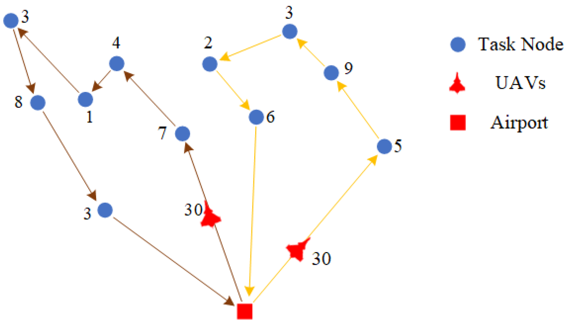
As shown in Figure 1, in the multi-UAV path planning and task allocation problem, the UAV-CVRP (Unmanned Aerial Vehicle Capacitated Vehicle Routing Problem) is a critical optimization challenge with widespread applications, particularly in ground missions such as reconnaissance and airdrop operations. Each UAV departs from the airport, executes a designated number of tasks, and returns to the airport for payload replenishment before depleting its capacity, continuing this process until all mission node demands are fulfilled. The demand at each mission node varies, and each node can only be serviced once. Throughout this process, UAV routes must be strategically planned to ensure that all task requirements are met while minimizing the total travel distance.

The airport is located at coordinates $P_0=(x_0,y_0,z_0)$, while the mission nodes are positioned at $P_i=(x_i,y_i,z_i)$ for $i\in 1,2,\dots ,n$. Each mission node $P_i$ requires a payload amount of $d_i$. The system consists of Q UAVs, each with a maximum payload capacity of C, meaning that the payload carried by a UAV during its mission cannot exceed C. The current position of a UAV is denoted as $p_k$ for $k\in 1,2,\dots ,Q$, and its current remaining payload is represented as $\widehat{C}$, satisfying the constraint $\widehat{C}\le C$.

The UAV’s path consists of a series of mission nodes, where each mission node can only be visited once. This path planning problem can be modeled using graph theory, where the mission nodes and the airport form the vertices of the graph. The movement of a UAV from one mission node to another corresponds to a path in the graph. The system’s state space is defined by the UAV’s position, current payload, and the demands of the mission nodes, which can be represented as $s=(p_k,\widehat{C},\{P_1,d_1,P_2,d_2,\dots ,P_n,d_n\})$.

In the decision-making process, the UAV needs to choose the next action target, which can be either heading towards a specific mission node or returning to the airport for replenishment. If the UAV chooses to execute a task at mission node $P_i$, it needs to consume the corresponding payload $d_i$, and the payload state is updated after the task is completed. The overall optimization objective is to minimize the total path length of all UAVs while meeting the demands of all mission nodes. The total path length calculation considers not only the journey of the UAV from the airport to the task nodes and executing tasks, but also the return to the airport after completing the tasks. Therefore, the optimization objective function can be expressed as follows:

$$min\sum _{k=1}^Q\left(\sum _{t=1}^{T_k}{d}_{k,t}\right)$$

(1)

where Q is the number of UAVs, $T_k$ is the number of path segments of the k-th UAV, and $d_{k,t}$ represents the distance between the mission nodes for the t-th segment of the path.

To ensure the successful execution of the tasks, the problem is subject to a series of constraints. First, each task node must be visited exactly once by a UAV, which can be expressed as follows:

$$\sum _{k=1}^Q\sum _{t=1}^{T_k}\mathbb{I}\left({\pi }_{k,t}=P_i\right)=1,\forall i\in \{1,2,\dots ,n\}$$

(2)

where $\mathbb{I}({\pi }_{k,t}=P_i)$ is an indicator function that indicates whether the path ${\pi }_{k,t}$ passes through the task node $P_i$. Additionally, during task execution, the remaining load of the UAV must be greater than or equal to the demand of the current task node; otherwise, the UAV must return to the airport for resupply:

$$\widehat{C}\ge d_i,\mathrm{if}{\pi }_{k,t}=P_i,\forall k\in \{1,\dots ,M\},\forall i\in \{1,\dots ,n\}$$

(3)

Moreover, the UAVs’ paths must satisfy payload constraints, meaning that the total load of task nodes assigned to each UAV must not exceed its maximum payload capacity. Additionally, all UAVs are required to return to the depot upon task completion.

$$\sum _{t=1}^{T_k}{d}_{k,t}\le C,\forall k\in \{1,\dots ,M\}$$

(4)

After determining the task sequences for all nodes using algorithms, all UAVs can operate along their respective closed-loop planned routes. This approach enables coordinated multi-UAV execution, ensuring the effectiveness of the overall routing strategy, while also allowing for parallel operations to reduce the total mission time for each individual UAV.

The core objective is to achieve efficient path planning that minimizes the total travel distance required to fulfill all task demands, under limited payload constraints. At the same time, the approach ensures the uniqueness of task execution, rational allocation of payloads among UAVs, and the overall feasibility of the generated paths.

3. Materials and Methods

In this chapter, we provide a detailed description of our proposed solution to the multi-UAV path planning problem. We define the solution strategy as a sequence of task node permutations, represented as $\mathit{\pi }=\left({\pi }_1,{\pi }_2,\dots ,{\pi }_n\right)$. To address the path planning problem, we introduce a probabilistic policy in state s as shown in Equation (5), where $\theta$ represents the learnable parameters. The term $p_{\theta }\left({\pi }_t\mid s,{\mathit{\pi }}_{1:t-1}\right)$ denotes the conditional probability of selecting the t-th task node ${\pi }_t$, given the current state and the previously selected sequence of task nodes $\mathit{\pi }1:t-1$. The policy is formally defined as follows:

$$p_{\theta }(\mathit{\pi }\mid s)=\prod _{t=1}^n{p}_{\theta }\left({\pi }_t\mid s,{\mathit{\pi }}_{1:t-1}\right)$$

(5)

We design a deep learning model to approximate this probabilistic distribution. Specifically, inspired by the solution proposed in [27], our model adopts an encoder–decoder architecture.

The encoder is responsible for embedding key information of all task nodes, which includes not only the features of the task nodes themselves but also the location of the depot and the remaining payload capacity of the UAVs. Utilizing a multi-head attention (MHA) mechanism, the encoder extracts useful contextual information from the relationships among task nodes, thereby generating embeddings for each node. The decoder sequentially selects task nodes based on the current state. At each decision step, it relies on the previously selected node sequence ${\mathit{\pi }}_{1:t-1}$ and updates the planned route accordingly. To prevent revisiting the same task node, we employ a masking mechanism during decoding, ensuring that already visited nodes are not selected again. By progressively selecting nodes, the decoder constructs the execution sequence of tasks while computing the corresponding probability distribution at each step.

To optimize the model parameters $\theta$, we employ a reinforcement learning-based training approach, specifically integrating the Multi-Start Greedy Rollout strategy with Baseline REINFORCE. A Multi-Start greedy strategy is used to select the next optimal task node for each UAV iteratively. Across multiple trials, the Multi-Start Greedy Rollout serves as a baseline method to evaluate the model performance. After each route selection, a reward function is computed based on the total path length and task completion status. The reward function is designed to encourage the model to minimize the path length while satisfying task constraints. The REINFORCE algorithm is utilized to estimate gradients of the loss function, enabling backpropagation to update the model parameters $\theta$. In each iteration, the model refines its policy by computing probability distributions and adjusting parameters based on the rewards obtained from actual path lengths.

Through the aforementioned approach, we optimize the parameters $\theta$ in the multi-UAV path planning problem, enabling the model to effectively minimize the total path length while ensuring that the task requirements of each node are met in real-world applications.

3.1. Multi-Head Attention (MHA)

Multi-head attention (MHA) has been widely adopted in neural network models, and the Graph Attention Network proposed in [34] has demonstrated its effectiveness. In this study, we also employ the multi-head attention mechanism, allowing nodes to receive heterogeneous information from multiple task-relevant nodes, thereby enhancing the ability of the model to capture complex relationships.

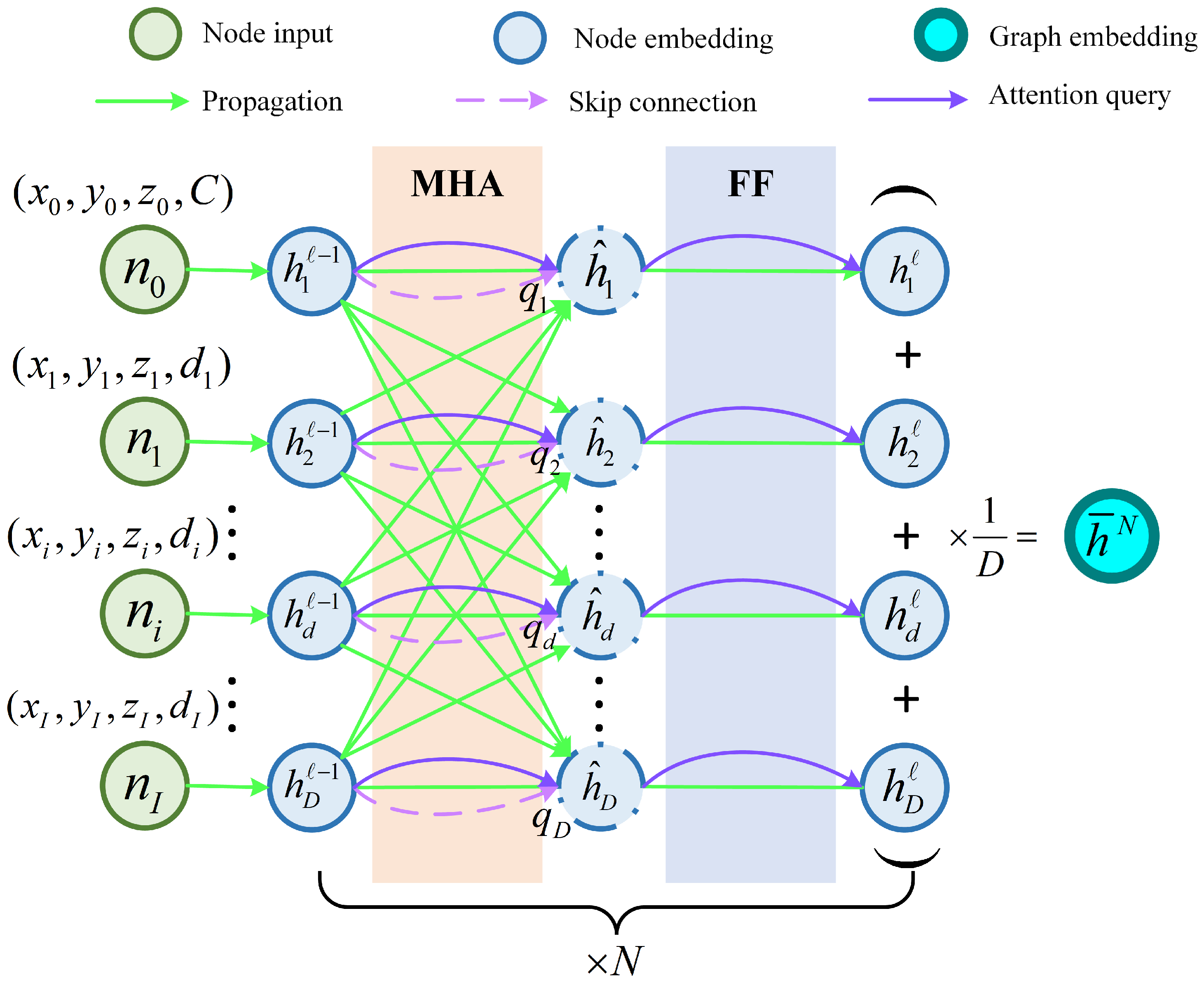
As illustrated in Figure 2, following the approach of [28], the attention mechanism can be interpreted as a weighted message passing process within the task node graph. In this framework, the weight assigned to the message received by a node from its neighbors is determined by the relevance between its query and the key of the neighboring nodes. Let $d_k$ and $d_v$ represent the dimensions of the key and value representations, respectively. The key ${\mathbf{k}}_i$, value ${\mathbf{v}}_i$, and query ${\mathbf{q}}_i$ for each node are computed by projecting its embedding ${\mathbf{h}}_i$ as follows:

$${\mathbf{q}}_i=W^Q{h}_i,{\mathbf{k}}_i=W^K{h}_i,{\mathbf{v}}_i=W^V{h}_i$$

(6)

Here, the projection matrices $W^Q$ and $W^K$ are of size $d_k\times d_h$, while $W^V$ is of size $d_v\times d_h$. Based on the computed queries and keys, we define the relevance score $u_{ij}$ between node i and node j as the scaled dot product of the query ${\mathbf{q}}_i$ and the key ${\mathbf{k}}_j$:

$$u_{ij}=\left\{\begin{array}{cc}{\displaystyle \frac{{\mathbf{q}}_i^T{\mathbf{k}}_j}{\sqrt{d_{\mathbf{k}}}}}\hfill & otherwise,\hfill \\ -\infty \hfill & i=j\hfill \end{array}\right.$$

(7)

To prevent self-interaction, we assign a score of $-\infty$ to $u_{ij}$ when $i=j$, ensuring that a node does not attend to itself. The attention weights $a_{ij}\in [0,1]$ are then computed using the softmax function $a_{ij}={\displaystyle \frac{e^{u_{ij}}}{{\sum }_{j^{\prime }}{e}^{u_{i{j}^{\prime }}}}}$.

Finally, the node embedding $h_i^{\prime }$ is updated using the equation $h_i^{\prime }={\sum }_j{a}_{ij}{\mathbf{v}}_j$, where the attention weights $a_{ij}$ determine the contribution of each neighboring node.

Let M denote the number of attention heads, where each head has independent parameters that satisfy the dimensional constraint $d_k=d_v={\displaystyle \frac{d_h}{M}}=16$. For each node i, the output representation of the $m$-th attention head is denoted as $h_{im}^{\prime }$, where $m\in 1,\dots ,M$. Subsequently, a projection matrix $W_m^O$ (of dimensions $d_h\times d_v$) is applied to transform the outputs of all attention heads, integrating the information into a unified $d_h$-dimensional space. Finally, the multi-head attention representation of node i, denoted as MHA_i, is computed as the weighted sum of the outputs from all attention heads:

$${MHA}_i\left({\mathbf{h}}_1,\dots ,{\mathbf{h}}_n\right)=\sum _{m=1}^M{W}_m^O{\mathbf{h}}_{im}^{\prime }$$

(8)

This formulation ensures that information from different attention heads is effectively integrated after transformation, providing a richer feature representation for subsequent learning tasks.

3.2. Encoder Based on MHA

The encoder employed in this work (Figure 3) follows a structure similar to that of the transformer encoder. However, positional encoding is omitted to ensure that the resulting node embeddings remain invariant to the input order.

The input to the encoder consists of the feature set of all nodes, as defined in Equation (9). The airport node is positioned at the beginning of the input sequence, with its feature representation given by ${\mathbf{n}}_0$; each task node is characterized by its spatial coordinates and task demand, represented as ${\mathbf{n}}_i(i\in 1,\dots ,n)$.

$${\mathbf{n}}_i=\left\{\begin{array}{cc}{P}_0,C\hfill & i=0\hfill \\ P_i,d_i\hfill & i=1,\dots ,n\hfill \end{array}\right.$$

(9)

The primary function of the encoder is to transform the input feature into hidden embeddings $\mathbf{h}$. To achieve this, separate learnable parameters $W,b$ are utilized to compute the initial embedding for both the airport node and task nodes. The mapping from input nodes to node embeddings is given by

$${\mathbf{h}}^0=\left\{\begin{array}{cc}{W}_0{\mathbf{n}}_i+b_0\hfill & i=0\hfill \\ W{\mathbf{n}}_i+b\hfill & i=1,\dots ,n.\hfill \end{array}\right.$$

(10)

The embeddings undergo refinement through N layers of multi-head attention, with each layer comprising two distinct sublayers. The first sublayer, a multi-head attention (MHA) mechanism, enables effective message passing among nodes, while the second sublayer, a Fully Connected Feed-Forward (FF) network, processes each node independently. To enhance training stability and accelerate convergence, both sublayers integrate residual connections and batch normalization (BN). The updated node embeddings are computed as follows:

$$\begin{array}{cc}\hfill {\widehat{\mathbf{h}}}_d& ={\mathrm{BN}}^{\ell }\left[{\mathbf{h}}_d^{\ell -1}+{MHA}_d^{\ell }\left({\mathbf{h}}_1^{\ell -1},\dots ,{\mathbf{h}}_D^{\ell -1)}\right)\right],\hfill \end{array}$$

(11)

$$\begin{array}{cc}\hfill {\mathbf{h}}_d^{\ell }& ={\mathrm{BN}}^{\ell }\left[{\widehat{\mathbf{h}}}_d+{\mathrm{FF}}^{\ell }\left({\widehat{\mathbf{h}}}_d\right)\right].\hfill \end{array}$$

(12)

This attention mechanism efficiently captures both local and global contextual information, allowing the model to produce high-quality embeddings for the decoding process. The node embedding generated by the ℓ-th attention layer is represented as $h_d^{\ell }$, where $\ell \in 1,\dots ,N$, and the subscript d denotes the embedding of the d-th node at this layer. To summarize the graph representation, the encoder computes an aggregated embedding, ${\overline{h}}^{\left(N\right)}$, by averaging the final node embeddings.

$${\overline{\mathbf{h}}}^N={\displaystyle \frac{1}{D}}\sum _{i=1}^D{\mathbf{h}}_d^N.$$

(13)

where D represents the hidden layer dimension. Both the final node embeddings $h_d^N$ and the graph-level embedding ${\overline{h}}^{\left(N\right)}$ serve as inputs to the decoder.

3.3. Decoder for Path Sequences

The decoder operates sequentially, where the output at time step t depends on the output at time $t-1$ and the current state. The generated trajectory starts at the depot and must return to the depot to ensure a closed tour. At the initial decoding step, the context node embedding is formed by combining the graph embedding ${\overline{\mathbf{h}}}^N$, the depot node embedding $\mathbf{h}{0}^N$, and the remaining capacity $\widehat{C_t}$. In subsequent steps, this context embedding is dynamically updated by integrating the graph embedding ${\overline{\mathbf{h}}}^N$, the embedding of the previously selected node $h^N{\pi }_{t-1}$, and the remaining capacity $\widehat{C_t}$.

$${\mathbf{h}}_c^N=\left\{\begin{array}{cc}\left[{\overline{\mathbf{h}}}^N,{\mathbf{h}}_{{\pi }_{t-1}}^N,\widehat{C_t}\right]\hfill & t>1\hfill \\ \left[{\overline{\mathbf{h}}}^N,{\mathbf{h}}_0^N,\widehat{C_t}\right]\hfill & t=1\hfill \end{array}\right.$$

(14)

where $[·,·,·]$ denotes the concatenation operator. The concatenated vector is denoted as ${\mathbf{h}}_c^N$ to highlight its role as a specialized embedding combining contextual information and graph embeddings. The dimensionality of ${\mathbf{h}}_c^N$ is $3\times d_{\mathbf{h}}$. The embedding ${\mathbf{h}}_c^N$ is then projected back to the original $d_{\mathbf{h}}$ dimensional space using a learned transformation; use ${\mathbf{q}}_c=W^Q{\mathbf{h}}_c$.

This results in the query vector ${\mathbf{q}}_c^N$ for the concatenated embedding ${\mathbf{h}}_c^N$. We then compute the compatibility between ${\mathbf{q}}_c^N$ and the embeddings of other nodes using the multi-head attention mechanism described in Section 3.1, obtaining a new contextual feature embedding ${\mathbf{h}}_c^{N+1}$. Notably, this step only involves computing the specialized contextual embedding and does not require updating the embeddings of other nodes.

Next, we compute the final output probability $p_{\theta }\left({\pi }_t\right|s,{\pi }_{1:t-1})$, where ${\pi }_t$ is the index of the node selected at decoding step t. A single-head attention layer is used to compute the value scores $v_{cj}$. Following Bello et al. [25] and Kool et al. [27], we apply a clipping operation within the range $[-L,L]$ (where $L=10$) using the tanh function as follows:

$$u_{cj}=\left\{\begin{array}{cc}L·tanh\left({\displaystyle \frac{{\mathbf{q}}_c^T{\mathbf{k}}_j}{\sqrt{d_k}}}\right)\hfill & \mathrm{if}j\ne {\pi }_{t^{\prime }}\forall t^{\prime }<t\hfill \\ -\infty \hfill & \mathrm{otherwise}.\hfill \end{array}\right.$$

(15)

Here, we mask out nodes that are inaccessible at time t by setting their corresponding $u_{cj}$ values to $-\infty$. This ensures that previously visited nodes are excluded from selection. The computed compatibility scores are treated as unnormalized log probabilities (logits), and the final probability distribution is derived by applying the softmax function.

$$p_i=p_{\mathit{\theta }}\left({\pi }_t=i\mid s,{\mathit{\pi }}_{1:t-1}\right)={\displaystyle \frac{e^{u_{ci}}}{{\sum }_j{e}^{u_{cj}}}}.$$

(16)

To ensure compliance with the UAV’s capacity constraints, we monitor the task demands ${\widehat{d}}_{i,t}$ for each node $i\in \{1,\dots ,n\}$ and the available vehicle capacity ${\widehat{C}}_t$ at time step t. Initially, at $t=1$, these values are set as ${\widehat{d}}_{i,t}={\widehat{d}}_i$ and ${\widehat{C}}_t=C$. Subsequently, they are updated based on the following rules:

$$\begin{array}{cc}\hfill & {\widehat{d}}_{i,t+1}=\left\{\begin{array}{cc}0\hfill & {\pi }_t=i\hfill \\ {\widehat{d}}_{i,t}\hfill & {\pi }_t\ne i\hfill \end{array}\right.\hfill \\ \hfill & {\widehat{C}}_{t+1}=\left\{\begin{array}{cc}max\left({\widehat{C}}_t-{\widehat{d}}_{{\pi }_t,t},0\right)\hfill & {\pi }_t\ne 0\hfill \\ C\hfill & {\pi }_t=0\hfill \end{array}\right.\hfill \end{array}$$

(17)

3.4. Reinforcement Learning Algorithm

In the previous section, we derived the probability of each node, allowing us to construct a complete trajectory probability distribution as follows:

$$p_{\theta }(\pi \mid s)=\prod _{t=1}^n{p}_{\mathit{\theta }}\left({\pi }_t\mid s,{\pi }_{1:t-1}\right).$$

(18)

Meanwhile, we define $L\left(\mathit{\pi }\right)$ as the expected total length of the UAV task route. The objective of model training is to minimize this expected path length. We also define $R\left(\mathit{\pi }\right)$ as the reward associated with a given policy, and following the approach proposed by Kool et al. [27], we set $R\left(\mathit{\pi }\right)=-L\left(\mathit{\pi }\right)$. Thus, the reinforcement learning task is to optimize the policy $\mathit{\pi }$ such that the expected reward $R\left(\mathit{\pi }\right)$ is maximized, which leads to the maximization of the following objective function:

$$\mathcal{L}(\mathit{\theta }\mid s)={\mathbb{E}}_{p_{\mathit{\theta }}(\pi \mid s)}\left[R\left(\mathit{\pi }\right)\right]$$

(19)

By optimizing this objective using gradient descent, we obtain the classical policy gradient (REINFORCE):

$$\nabla \mathcal{L}(\mathit{\theta }\mid s)={\mathbb{E}}_{p_{\mathit{\theta }}(\mathit{\pi }\mid s)}\left[R\left(\mathit{\pi }\right)\nabla log{p}_{\mathit{\theta }}(\mathit{\pi }\mid s)\right]$$

(20)

However, this approach suffers from high variance, leading to instability during training. To mitigate variance in gradient estimation, a baseline function $b\left(s\right)$ can be introduced, modifying the policy gradient as follows:

$$\nabla \mathcal{L}(\mathit{\theta }\mid s)={\mathbb{E}}_{p_{\mathit{\theta }}(\mathit{\pi }\mid s)}\left[(R\left(\mathit{\pi }\right)-b\left(s\right))\nabla log{p}_{\mathit{\theta }}(\mathit{\pi }\mid s)\right]$$

(21)

Since the baseline $b\left(s\right)$ is independent of the specific trajectory $\pi$, it does not affect the unbiased nature of the gradient. Incorporating this baseline effectively reduces gradient variance and enhances training efficiency.

A common choice for the baseline in reinforcement learning is the state-value function, defined as follows:

$$b\left(s\right)=V^{\pi }\left(s\right)={\mathbb{E}}_{\pi }[R\mid s]$$

(22)

which represents the expected cumulative return when following policy $\pi$ from state s. However, computing $V\left(s\right)$ is challenging due to the unknown state transitions in the environment and the infeasibility of explicitly enumerating all possible future trajectories.

As illustrated in Figure 4, we adopt the Multi-Start Greedy Rollout method as the baseline. For each state s, multiple greedy searches are performed from different random starting points, and the trajectory yielding the highest return is selected as the baseline value $b\left(s\right)$, computed as shown in Equation (23). The objective of this algorithm is to optimize a reinforcement learning policy using the REINFORCE policy gradient method, while leveraging the Multi-Start Greedy Rollout to construct a strong baseline that reduces variance and accelerates convergence.

$$b\left(s\right)=arg\underset{{\pi }_i\in {\pi }_1,{\pi }_2,...,{\pi }_K}{min}R\left({\pi }_i\right),$$

(23)

Specifically, the process begins by sampling problem instances from a given distribution and converting them into state representations, which are then fed into the policy network. Under the current policy parameterized by $\theta$, a feasible solution ${\pi }_i$ is sampled, and its corresponding return $R\left({\pi }_i\right)$ is evaluated. Meanwhile, a separate baseline policy with parameters ${\theta }^{BL}$ performs multiple greedy rollouts on the same state, generating several candidate solutions. Among these, the one with the highest return is selected as the baseline solution ${\pi }_i^{BL}$. The return difference between the sampled solution and the baseline solution is then used to compute the policy gradient, which updates the policy network to maximize the expected return. This process strikes a balance between exploration and exploitation, while the dynamically updated, high-quality baseline policy provides a stable and informative learning signal.

During training, as model parameters continuously evolve, we freeze the Multi-Start Greedy Rollout policy $p_{{\mathit{\theta }}^{\mathrm{BL}}}$ within each epoch to ensure the stability of $b\left(s\right)$. At the end of each epoch, the current training policy is compared against the baseline policy using Multi-Start Greedy decoding, and a paired t-test ($\alpha =5\%$) is conducted to evaluate whether the performance improvement is statistically significant. If the improvement is significant, the current policy parameters $\mathit{\theta }$ replace the baseline policy parameters ${\mathit{\theta }}^{\mathrm{BL}}$; otherwise, the baseline remains unchanged.

When employing Multi-Start Greedy Rollout as the Baseline $b\left(s\right)$, if the target value $R\left(\mathit{\pi }\right)-b\left(s\right)$ for a sampled solution $\pi$ is positive (indicating an improvement over the Multi-Start Greedy Rollout), the selection probability of $\pi$ is reinforced. Conversely, if $R\left(\mathit{\pi }\right)-b\left(s\right)$ is negative (indicating worse performance than the Multi-Start Greedy Rollout), the selection probability is reduced. This mechanism encourages the model to continuously surpass its own Multi-Start Greedy solutions, thereby improving policy performance. The algorithmic procedure is detailed in Algorithm 1, and the calculation formula of MultiStartGreedyRollout is $\mathrm{MultiStartGreedyRollout}(s,p_{{\theta }^{BL}},K)=arg{min}_{\pi \in \{{\pi }_1,...,{\pi }_K\}}R\left(\pi \right)$.

Algorithm 1 REINFORCE with Multi-Start Greedy Rollout Baseline

1: Input: number of epochs E, steps per epoch T, batch size B, significance α

2: Init $\theta ,{\theta }^{BL}\leftarrow \theta$

3: for epoch = 1, …, E do

4:       for step = 1, …, T do

5:              $s_i\leftarrow \mathrm{RandomInstance}\left(\right) \forall i\in \{1,\dots ,B\}$

6:              ${\pi }_i\leftarrow \mathrm{SampleRollout}(s_i,p_{\theta }) \forall i\in \{1,\dots ,B\}$

7:              ${\pi }_i^{\mathit{BL}}\leftarrow \mathrm{MultiStartGreedyRollout}(s_i,p_{{\theta }^{\mathit{BL}}},K)$

8:              $\nabla \mathcal{L}\leftarrow {\sum }_{i=1}^B \left(R\right({\pi }_i-R\left({\pi }_i^{\mathit{BL}}\right)\left){\nabla }_{\theta }\log p_{\theta }\right({\pi }_i)$

9:              $\theta \leftarrow \mathrm{AdamW}(\theta ,\nabla \mathcal{L})$

10:       end for

11:       if OneSidedPairedt-Test ($p_{\theta },p_{{\theta }^{\mathit{BL}}}) < \alpha$ then

12:              ${\theta }^{\mathit{BL}}\leftarrow \theta$

13:       end if

14: end for

4. Results

In this section, we describe a series of systematic experiments conducted to comprehensively evaluate the performance of the proposed model in multi-UAV task planning. First, we employed experiments to identify the most robust optimal hyperparameter configuration, ensuring the stability of the model and generalization capability. Subsequently, we compared the optimized model with widely adopted exact solvers and heuristic algorithms in the field of route planning, including Gurobi [7], genetic algorithm (GA) [35], Particle Swarm Optimization (PSO) [36], and Ant Colony Optimization (ACO) [37], to analyze its performance across different task scales.

Furthermore, to further investigate the impact of model architecture on task planning effectiveness, we systematically replaced the encoder module, decoding strategy, and reinforcement learning baselines to assess their individual contributions to solution quality. For the encoder, we evaluated alternative designs based on Graph Convolutional Networks (GCNs) and Message Passing (MP) networks [38]. For the decoding strategy, we compared the performance of Greedy Search, Sampling, and Beam Search [39]. We also experimented with different reinforcement learning baseline strategies, including no baseline, Advantage Actor–Critic (A2C) [40], and Soft Actor–Critic (SAC) [38], to explore how varying search strategies influence both the quality of solutions and computational efficiency.

Finally, we assessed the generalization capability of our model across multiple real-world scenarios by conducting experiments in simulated mountainous environments and testing on instances derived from real-world terrain data obtained from Google Earth.

4.1. Experimental Setting

In the training phase, consistent with prior studies, we dynamically and independently generate the positions of all training samples (including depot and task nodes) using a two-dimensional uniform distribution within the range $[0,1]$. The distance between any two nodes is calculated based on the Euclidean metric. Each model under evaluation is trained for 200 epochs, with 1,000,000 instances generated and trained per epoch. For validation, a randomly sampled set of 100,000 instances is used to evaluate model performance. All training procedures were accelerated by GPU using twoNvidia RTX 4090 GPUs (NVIDIA Corporation, Santa Clara, CA, USA) and anAMD EPYC 9534 64-Core CPU (Advanced Micro Devices, Inc., Santa Clara, CA, USA).

In the subsequent experimental phase, we demonstrate the effectiveness of our model on a fixed benchmark test set, as shown in

Table 1. Fixed benchmark instances.

	Number of Instances	Number of Nodes	Random Generation	Real-World Scenarios
Comparative Experiment	512	10	T	F
	512	20	T	F
	512	50	T	F
	512	75	T	F
	512	100	T	F
Generalization Experiment	128	100	T	F
	30	25	F	T
	30	81	F	T

. To ensure fairness in performance comparison, all baseline methods and our model were evaluated on a CPU. The experimental codebase was implemented using Python 3.9, with PyTorch version 2.6 as the primary deep learning framework.

In the experimental phase, model hyperparameters—including optimizer type, learning rate, batch size, the number of initializations in the multi-start greedy method, the number of attention heads, and the number of attention layers—are determined through sensitivity analysis. This process enables the identification of the optimal parameter settings for the multi-UAV task planning problem and ensures the robustness of the model across varying conditions.

As this study does not focus on the development of heuristic algorithms, the parameter configurations for the exact and heuristic baseline algorithms were directly adopted from the open-source library provided in [41]. This ensured a fair experimental comparison and reduced the variability caused by manual tuning.

4.2. Parameter Sensitivity Experiment

The parameter sensitivity experiment was designed to analyze the model’s sensitivity to variations in different parameters. In this section, we modified the hyperparameters of the model to observe their effects on performance and output results, aiming to evaluate the importance of these parameters in the system’s performance. Ultimately, this allowed us to identify the optimal parameter combination.

To ensure fairness, all hyperparameters except those involved in the sensitivity analysis were kept fixed. We evaluated the validation performance of the greedy decoder on 20-node and 50-node instances across three different random seeds. The experiments investigated the sensitivity of training batch size, optimizer type, learning rate, number of attention layers, number of attention heads, and the number of multi-start initializations. It is worth noting that under identical experimental settings, we set the random seeds to (40, 41, 42), respectively. This setup allows for a clearer understanding of parameter sensitivity across different random seeds. In this subsection, all validation results are reported as the mean cost over the three random seeds, and we also provide the standard deviation to quantify variability. The error bands in the experimental result plots (Figure 5) reflect these deviations.

Additionally, testing was conducted on a fixed test set comprising 2048 samples, each generated randomly. For each test, 20 and 50 task nodes were generated, with drone capacities set to 1 and task demands randomly assigned values between 0 and 1. The models participating in the sensitivity experiments were evaluated on this test set. The test results include the outcomes of models trained with three different random seeds, along with their mean values. The testing results on the fixed test set are presented in

Table 2. Parameter sensitivity experimental results under different node settings.

Parameter	Node = 20				Node = 50
	Seed = 40	Seed = 41	Seed = 42	Average	Seed = 40	Seed = 41	Seed = 42	Average
Batch_size = 128	9.6493	9.6496	9.6697	9.6562	17.8113	17.6878	17.7254	17.7415
Batch_size = 256	9.6154	9.6075	9.6116	9.6115	17.8954	17.6973	17.4044	17.6657
Batch_size = 512	9.5379	9.5763	9.5738	9.5627	17.6290	17.6703	17.6611	17.6535
Batch_size = 1024	9.5879	9.5936	9.5957	9.5924	17.6501	17.6355	17.6893	17.6583
SGD	9.6413	9.6377	9.6632	9.6474	17.6955	17.7816	17.7726	17.7499
Adam	9.5968	9.5874	9.5951	9.5931	17.6637	17.6198	17.5957	17.6264
AdamW	9.5379	9.5763	9.5738	9.5627	17.6290	17.6703	17.6611	17.6535
$\eta$ = 1 × 10−3	9.5379	9.5763	9.5738	9.5627	17.6290	17.6703	17.6611	17.6535
$\eta$ = 1 × 10−4	9.5789	9.5758	9.5847	9.5798	17.7770	17.7189	17.7395	17.7451
N = 2	9.5764	9.5734	9.5625	9.5708	17.7125	17.6957	17.7848	17.7310
N = 3	9.5622	9.5440	9.6021	9.5694	17.6644	17.7047	17.6995	17.6895
N = 4	9.5379	9.5763	9.5738	9.5627	17.6290	17.6703	17.6611	17.6535
N = 5	9.5858	9.5723	9.5529	9.5703	17.7376	17.6627	17.6861	17.6955
M = 4	9.6228	9.6464	9.6088	9.6260	17.8851	17.7806	17.8249	17.8302
M = 8	9.5379	9.5763	9.5738	9.5627	17.6290	17.6703	17.6611	17.6535
M = 16	9.5473	9.5496	9.5500	9.5490	17.6322	17.5993	17.5994	17.6103
K = 4	9.4913	9.7097	9.6965	9.6325	17.7536	17.6937	17.7538	17.7337
K = 8	9.58	9.6021	9.5849	9.589	17.8534	17.5233	17.6132	17.6633
K = 12	9.5379	9.5763	9.5738	9.5627	17.6290	17.6703	17.6611	17.6535

.

Based on the validation performance in Figure 5 and the statistical results in Table 2, we analyze the hyperparameters from the perspectives of robustness and solution quality.

A larger batch size tends to yield slightly better performance; specifically, batch sizes of 512 and 1024 produce lower path costs and exhibit less sensitivity to random seeds. However, the performance difference between the two is marginal. Considering the GPU memory limitations of the experimental hardware, we adopted a batch size of 512 as a practical choice. The AdamW optimizer demonstrated improved stability by incorporating appropriate weight decay, and the results showed that AdamW achieved better and more consistent optimization compared to other optimizers. In the learning rate sensitivity experiment, we compared two commonly used values: 1 × 10⁻³ and 1 × 10⁻⁴. Under the 20-node experimental setup (see Figure 5c), the learning rate of 1 × 10⁻³ exhibited faster convergence and slightly better final performance than 1 × 10⁻⁴. This difference became more pronounced in the 50-node setting (Figure 5i), where 1 × 10⁻³ converged more rapidly and achieved a significantly lower cost. Additionally, the error bands in the plots indicate that a learning rate of 1 × 10⁻³ provides greater robustness to variations in random seeds, showing lower sensitivity to stochastic perturbations.

For the sensitivity analysis on the number of attention layers, we tested four settings: 2, 3, 4, and 5 layers. In the 20-node environment, the performance across all settings was relatively similar. However, in the 50-node setting, the configuration with 4 layers yielded better results. Furthermore, the error bands indicate that the 4-layer configuration exhibits greater robustness with respect to random seed variation. From the sensitivity analysis on the number of attention heads for both 20-node and 50-node tasks, we observe that using 4 attention heads results in relatively poor performance, whereas models with 8 or 16 heads perform comparably. Notably, the model with eight attention heads demonstrates reduced sensitivity to random seed fluctuations and, thus, exhibits better robustness. Moreover, using 8 heads incurs a lower computational cost compared to 16. The number of multi-starts (K) is a critical hyperparameter in our framework. In the 20-node validation and test scenarios, both $K=8$ and $K=12$ achieved similar performance. However, for the 50-node tasks, larger values of K led to better results, albeit at the expense of an increased computational cost. Based on the comprehensive sensitivity analysis conducted on fixed test sets in both 20-node and 50-node environments, we conclude that the optimal and most robust configuration is as follows: batch size of 512, AdamW optimizer, learning rate $\eta$ =1 × 10⁻³, number of attention layers $N=4$, number of attention heads $M=8$, and number of greedy rollouts $K=12$. This combination yields strong performance while exhibiting the lowest sensitivity to random seed variations.

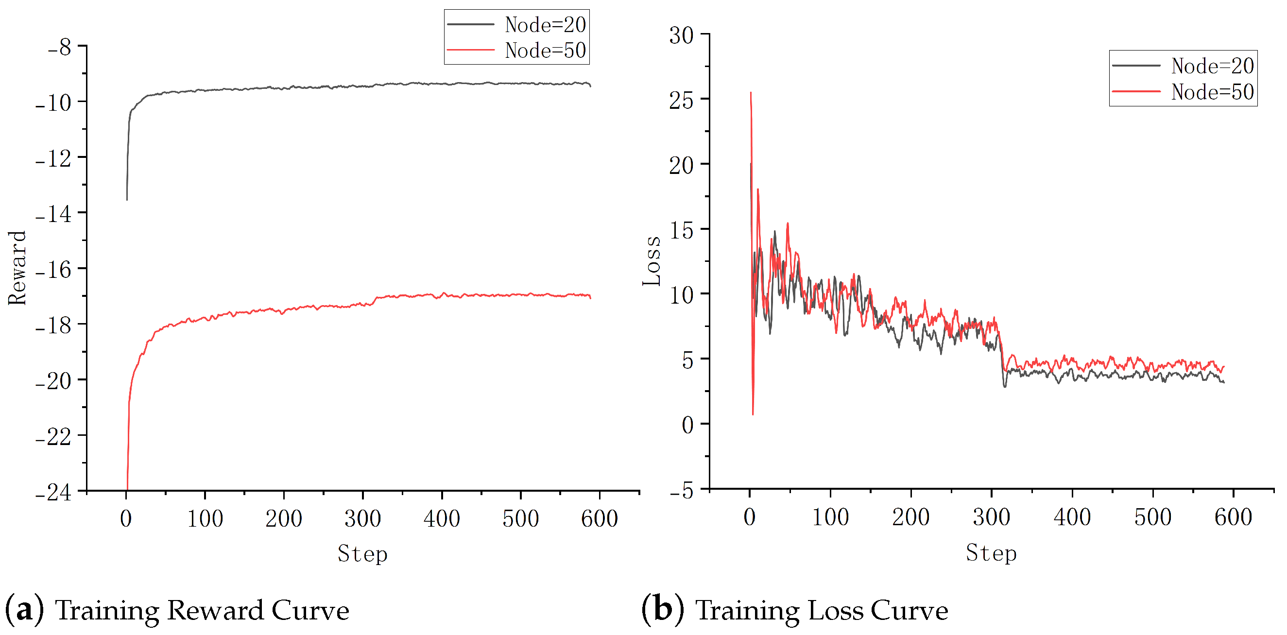
Additionally, under the confirmed optimal hyperparameter settings, we present the training curves in Figure 6, which illustrate the reward and loss trajectories for both problem scales. These curves are intended to analyze the convergence behavior of our model. It can be observed that the model achieves convergence within approximately 50 training epochs. However, a notable performance improvement occurs around epoch 310, which we attribute to the model learning more effective decision-making strategies at this stage of training.

4.3. Comparative Experiment

This section evaluates the superiority of the proposed algorithm on a fixed test set comprising five different task scales. We compare our method against traditional algorithms as well as models employing different encoder architectures, decoding strategies, and baseline methods. A comprehensive assessment is conducted with respect to both solution cost and inference time. For deep reinforcement learning-based models, the results are reported as the average over three random seeds. The comparative results are summarized in

Table 3. Model comparison experimental results under multiple task nodes. Due to the importance of efficiency in large-scale problems, we disregard longer inference times. Therefore, when using the exact solver Gurobi for inference, superscript * is used to indicate that the solution was obtained under a fixed time limit.

Method	Node = 10		Node = 20		Node = 50		Node = 75		Node = 100
	Cost	Time	Cost	Time	Cost	Time	Cost	Time	Cost	Time
Gurobi	3.6491	0.53 s	6.9077	>12 s	16.329	3 min *	47.6185	4 min *	63.5837	5min *
GA	3.7692	18.8 s	7.2725	>54 s	18.1856	>2 min	31.1014	>2 min	43.4577	>3 min
ACO	3.9317	20.44 s	7.1174	>1 min	17.0645	>3 min	28.896	>5 min	33.372	>8 min
DPSO	4.1525	18.97 s	8.9268	>1 min	25.884	>4 min	41.7249	>6 min	56.947	>8 min
GCN	5.0862	2.59 ms	9.4867	4.62 ms	17.1562	9.19 ms	23.5083	13.10 ms	28.5466	16.50 ms
MP	5.2077	2.81 ms	9.4366	4.61 ms	17.1021	9.19 ms	23.0825	12.90 ms	28.0417	16.80 ms
MHA	5.198	2.65 ms	9.3324	4.73 ms	17.0763	9.63 ms	22.7759	13.10 ms	27.5123	16.70 ms
Greedy	5.2407	2.49 ms	9.6244	3.75 ms	17.5551	6.83 ms	23.4723	10.10 ms	28.1369	13.80 ms
Sampling	5.1595	2.74 ms	9.6853	4.13 ms	17.887	8.23 ms	23.6158	12.10 ms	28.4348	16.10 ms
Beam	5.0328	3.06 ms	9.3367	7.45 ms	17.1885	13.60 ms	22.9018	19.60 ms	27.7307	24.90ms
Multi-start	5.198	2.65 ms	9.3324	4.73 ms	17.0763	9.63ms	22.7759	13.10 ms	27.5123	16.70 ms
No baseline	5.4943	2.03 ms	10.763	4.63 ms	19.6124	9.01ms	28.9716	11.93 ms	35.6437	15.19 ms
A2C	5.0176	2.79 ms	9.4563	4.79 ms	17.1576	9.97ms	21.9743	13.75 ms	26.7982	17.76ms
SAC	4.9117	2.94 ms	9.4952	4.91 ms	17.8676	10.35ms	21.5837	13.64 ms	27.9885	18.37 ms
Rollout baseline	5.198	2.65 ms	9.3324	4.73 ms	17.0763	9.63ms	22.7759	13.10 ms	27.5123	16.70 ms

.

For traditional algorithms, we selected representative methods commonly used for solving CVRP problems, including the exact solver Gurobi and heuristic algorithms such as genetic algorithm (GA), Ant Colony Optimization (ACO), and the DPSD algorithm. The evaluated encoder architectures include GCN, Message Passing (MP), and the proposed multi-head attention (MHA) model. Decoding strategies considered include Greedy, Sampling, Beam Search, and the proposed multi-start strategy. Baseline learning approaches include no baseline, Advantage Actor–Critic (A2C), Soft Actor–Critic (SAC), and the Rollout Baseline method adopted in this work.

The exact solver Gurobi is capable of providing optimal solutions for small-scale tasks (fewer than 20 nodes). It is evident that Gurobi fails to deliver optimal solutions within the allocated time for larger problem sizes.

Heuristic algorithms perform well on small-scale problems but exhibit significant performance degradation as the task size increases when compared to the proposed deep reinforcement learning approach. Specifically, even the best-performing heuristic method, Ant Colony Optimization (ACO), yields solutions with higher costs—by 5.8597 units—on 100-node problems relative to our proposed method. Furthermore, our approach demonstrates a substantial advantage in inference speed; heuristic algorithms require significantly longer computation times, particularly as the problem scale increases, further confirming the superiority of our model over traditional heuristics.

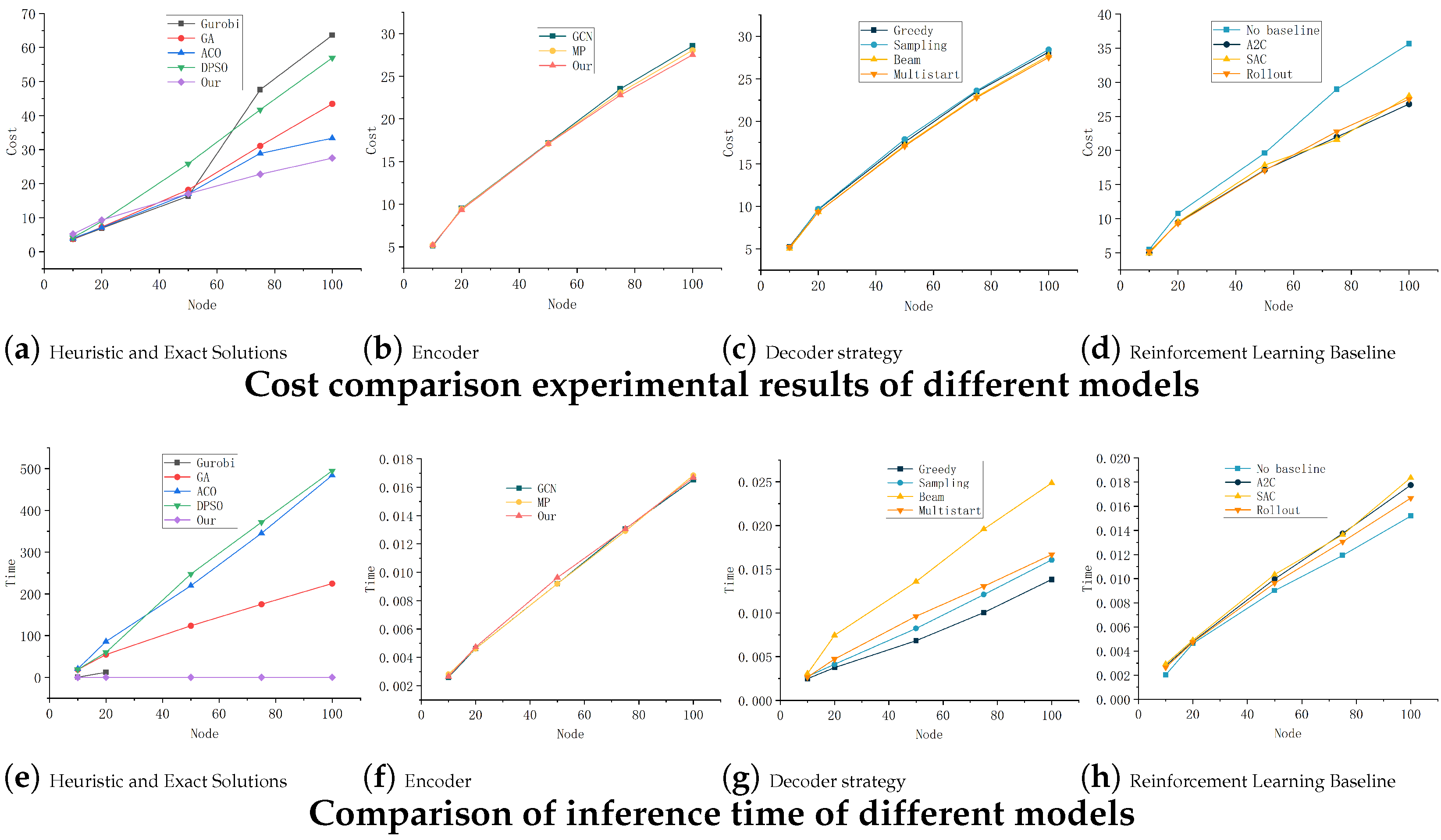
As illustrated in Figure 7, the proposed multi-head attention (MHA) encoder achieves the lowest cost under comparable inference times. The proposed multi-start decoding strategy consistently delivers the best cost performance across varying task sizes, with inference times on par with greedy and sampling-based decoders. While multi-start is not the fastest in terms of inference time, it offers the most favorable trade-off between solution quality and computational cost, as shown in Figure 7c,g.

In terms of baseline strategies, a clear performance gap exists between models trained with and without baseline learning. Although the model without baseline learning shows a slightly reduced inference time, it suffers in solution quality, achieving a cost of only 35.6437. When comparing widely used reinforcement learning baselines, such as A2C and SAC, the results remain similar among all three; however, the Rollout Baseline demonstrates clear advantages. Tailored to the fixed policy structure of CVRP solvers, it provides an approximately unbiased estimate and further improves inference speed.

In summary, while individual components of the model (encoders, decoders, and learning strategies) may show trade-offs in terms of speed or solution quality, the proposed method exhibits a consistent advantage across both performance and inference time dimensions. This comprehensive superiority validates the effectiveness of our approach in enhancing solution quality and computational efficiency across tasks of varying scale.

4.4. Generalization Experiment

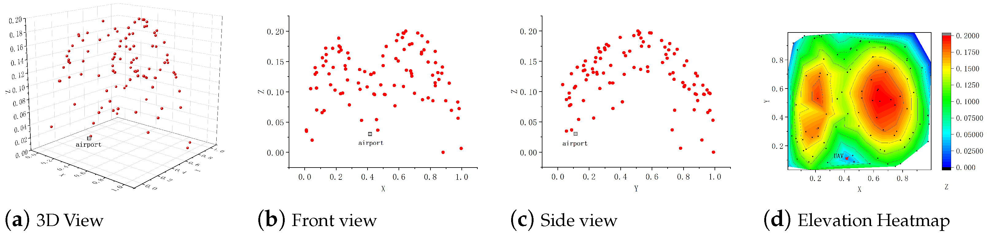
Generalization experiments were conducted across three scenarios: a numerical simulation (Figure 8), a 25-node real-world scenario, and an 81-node real-world scenario (Figure 9). The simulation involved 100 task points with demands ranging from 0.1 to 0.7 and a UAV capacity of 1. The real-world scenarios, based on normalized Google Earth coordinates, implemented reconnaissance and airdrop tasks. Reconnaissance, with zero task demand per node and a UAV capacity of 1, effectively became a traveling salesman problem (TSP). Airdrop tasks featured a UAV capacity of 30 and node demands randomly assigned between 5 and 15.

We also designed a dynamic heterogeneous task setting in a simulated scenario. To ensure fair evaluation across all models involved in the experiment, the following configuration was applied: the task demands of all task nodes were randomly generated, and the maximum capacity of each UAV was gradually degraded upon returning to the depot; the degradation rate was set to 5%. If the current maximum capacity of the UAV could no longer satisfy the minimum demand among the remaining task nodes, its capacity was reset to the original maximum value. All participating models were tested under this scenario.

The results of the generalization experiments are presented in

Table 4. Homogeneous and heterogeneous UAVs in simulated scenarios.

Method	Simulation A		Heterogeneous A
	Cost	Time	Cost	Time
GA	52.4577	>3 min	53.0587	>3 min
ACO	49.372	>8 min	51.6816	>9 min
DPSO	56.947	>8 min	59.6722	>9 min
GCN	47.3124	0.21 s	49.7119	>0.23 s
MP	46.5876	0.21 s	47.3138	>0.23 s
Greedy	46.7717	0.17 s	47.8326	>0.18 s
Sampling	48.8829	0.20 s	50.6394	>0.21 s
Beam	46.7586	0.31 s	47.5532	>0.33 s
A2C	47.3726	0.25 s	48.8865	>0.28 s
SAC	45.8262	0.38 s	46.4327	>0.39 s
Our	45.6129	0.21 s	46.0108	>0.22 s

and

Table 5. Performance comparison across different methods and scenarios.

Method	Reconnaissance B			Reconnaissance C			Airdrop B			Airdrop C
	Distance	Cost	Time	Distance	Cost	Time	Distance	Cost	Time	Distance	Cost	Time
GA	2.19 km	8.6195	>1 min	22.03 km	24.2076	>5 min	4.43 km	17.4253	>2 min	58.00 km	63.7345	>6 min
ACO	2.00 km	7.8499	>2 min	13.76 km	15.1253	>8 min	4.49 km	17.6372	>3 min	58.00 km	63.7363	>8 min
DPSO	2.24 km	8.8048	>2 min	24.64 km	27.0776	>6 min	4.73 km	18.6036	>2 min	50.50 km	55.49	>10 min
GCN	2.23 km	8.7603	0.03 s	14.76 km	16.2208	0.12 s	4.48 km	17.6301	0.06 s	48.98 km	53.8258	0.16 s
MP	1.78 km	6.9873	0.03 s	12.20 km	13.4095	0.12 s	4.48 km	17.6194	0.04 s	47.83 km	52.5595	0.16 s
Greedy	1.68 km	6.6160	0.03 s	11.89 km	13.0605	0.1 s	4.50 km	17.7013	0.04 s	47.80 km	52.5290	0.13 s
Sampling	1.74 km	6.8292	0.04 s	12.37 km	13.5879	0.12 s	4.51 km	17.7377	0.05 s	48.23 km	52.9986	0.15 s
Beam	1.63 km	6.3922	0.04 s	12.31 km	13.5260	0.18 s	4.42 km	17.3882	0.09 s	47.50 km	52.1987	0.24 s
A2C	1.72 km	6.7303	0.04 s	12.1 km	13.2949	0.15 s	4.44 km	17.4589	0.08 s	49.16 km	54.0229	0.22 s
SAC	1.63 km	6.3901	0.05 s	11.82 km	12.9892	0.18 s	4.40 km	17.2925	0.10 s	47.41 km	52.0927	0.26 s
Our	1.63 km	6.3921	0.04 s	11.82 km	12.9917	0.12 s	4.41 km	17.3492	0.06 s	47.13 km	51.79	0.16 s

. It is important to note that the "distance" column in the table represents the total path length of the UAV in the real-world scenario. The analysis reveals results similar to those observed in Section 3, where the proposed model achieves the best cost performance in the numerical simulation task. The inference time for a single instance is relatively low, and the deep reinforcement learning algorithm continues to show a significant performance advantage over heuristic algorithms in terms of inference speed. Additionally, the deep reinforcement learning algorithm demonstrates competitive performance in terms of path length.

We also visualized the path planning results for the reconnaissance and airdrop tasks in the real-world scenario with 25 nodes, as shown in Figure 9c,d. From the visualized UAV paths, it is clear that the model can effectively handle the complexities of real-world scenarios, generating complete node paths. In the airdrop task, the model ensures that the maximum load of the UAV and node task demand constraints are satisfied, while minimizing the path length required to complete the task. This demonstrates the true effectiveness and efficient generalization of the proposed model to cope with different types of tasks in real applications.

5. Discussion

This study addresses the increasing demand for efficient and scalable coordination of UAVs in complex operational environments, such as airdrop and reconnaissance missions. Traditional coordination methods are constrained by limitations in generalization, high inference times, and insufficient scalability, rendering them ineffective for large-scale multi-UAV planning tasks that require real-time decision-making, dynamic task allocation, and robust communication across multiple units.

To address these challenges, we propose an end-to-end deep reinforcement learning framework for multi-UAV path planning in 3D environments. This framework leverages an encoder–decoder architecture enhanced by multi-head attention and masking strategies to effectively model spatial relationships and optimize path planning. By autonomously learning strategies for dynamic task allocation and resource management, the model enhances scalability and adaptability in complex, real-time scenarios. Additionally, the integration of REINFORCE with a Multi-Start Greedy Rollout Baseline improves optimization stability, solution quality, and inference efficiency, thereby ensuring robust decision-making capabilities across multiple UAVs in time-sensitive operations.

Extensive experiments, including ablation studies, comparisons with heuristic algorithms, and evaluations on both simulated and real-world terrains using Google Earth data, demonstrate that the proposed method outperforms traditional approaches in terms of inference speed, solution quality, and generalization ability.

In future work, we will investigate multi-UAV task scheduling under time window constraints, with a focus on enhancing real-time decision-making capabilities and improving the scalability of task allocation. Additionally, we aim to explore distributed online inference in the context of integrated reconnaissance and strike missions, thereby strengthening the planning and problem-solving capacity of multi-UAV systems under dynamic conditions.