Generalising Rescue Operations in Disaster Scenarios Using Drones: A Lifelong Reinforcement Learning Approach

Abstract

Search and rescue (SAR) operations in post-earthquake environments are hindered by unseen environment conditions and uncertain victim locations. While reinforcement learning (RL) has been used to enhance unmanned aerial vehicle (UAV) navigation in such scenarios, its limited generalisation to novel environments, such as post-disaster environments, remains a challenge. To deal with this issue, this paper proposes an RL-based framework that combines the principles of lifelong learning and eligibility traces. Here, the approach uses a shaping reward heuristic based on pre-training experiences obtained from similar environments to improve generalisation, and simultaneously, eligibility traces are used to accelerate convergence of the overall approach. The combined contributions allows the RL algorithm to adapt to new environments, whilst ensuring fast convergence, critical for rescue missions. Extensive simulation studies show that the proposed framework can improve the average reward return by 46% compared to baseline RL algorithms. Ablation studies are also conducted, which demonstrate a 23% improvement in the overall reward score in environments with different complexities and a 56% improvement in scenarios with varying numbers of trapped individuals.

1. Introduction

Earthquake events have caused significant loss across the world, both for people’s lives and infrastructure. These natural disasters, depending of their magnitude, can lead to the collapse of buildings, trapping victims under debris, and modifying a city’s ecosystem. Immediate intervention is required to maximise the survivability of victims, as well as anticipate any potential earthquake replica. According to the CATDAT Damaging Earthquakes Database [1], the damage caused by high magnitude earthquakes is severe, such as in Haiti in 2010, where the median cost was around USD 7.8 billion, with an approximate fatality median of 137,000 people. These statistics underscore the need for the development of effective and timely search and rescue (SAR) operations that maximise the likelihood of survivability of victims after an earthquake event.

The incorporation of small autonomous vehicles has been transformative in SAR operations. For example, autonomous vehicles have been used to enter ruins with complex terrain for food delivery and to supply aid or identify targets in post-disaster event zones [2,3]. However, search and rescue missions in post-earthquake environments pose high uncertainty, which complicates the path-finding process to locate trapped victims. Traditional methods [4,5] have typically required prior knowledge of both the environment and the patient’s location [6], which limits their applicability in real-world implementations where such information might be unavailable.

1.1. Related Work

In earthquake-induced SAR operations, UAVs are particularly effective in identifying and locating trapped individuals in areas that are otherwise inaccessible to ground teams [7]. For instance, a cost-effective UAV system was developed to generate 3D point clouds from digital imagery, aiding in the detailed mapping of disaster sites [8]. This technology is essential in earthquake settings, where terrain is significantly altered, and immediate identification of potential rescue zones is crucial. UAVs have been applied in other disaster settings, such as floods and tsunamis [9,10], where the versatility of UAVs in SAR missions was demonstrated.

These aforementioned techniques can be directly transferred into earthquake scenarios, where accurate mapping and modelling of the environment are vital for rescue teams to operate effectively. Furthermore, UAVs have been utilised for simulating and predicting the impact of future disasters [11]. These approaches can also be adapted to earthquake settings, enhancing both pre-disaster preparedness and post-disaster response, thereby improving the overall effectiveness of SAR missions.

1.1.1. Path Planning Algorithms

Path planning plays a crucial role in SAR operations, especially in the unpredictable and often hazardous environments caused by earthquakes. Traditional methods, such as Dijkstra’s algorithm, have been widely used due to their ability to find the shortest path in a graph, which is an essential requirement for navigating disaster-stricken areas. However, Dijkstra’s algorithm is optimised for static environments and struggles to accommodate real-time updates in dynamic settings [12].

To address the limitations of static algorithms, $A^{*}$ and its variants have been adopted in SAR operations. $A^{*}$ is particularly effective due to its heuristic-based approach, which reduces computational complexity while maintaining efficient path-finding [13]. Notable applications of $A^{*}$ include its use in mapping and navigating urban disaster sites where both precision and computational efficiency are crucial. The hierarchical $A^{*}$ and Hybrid $A^{*}$ algorithms further enhance these capabilities by optimising the search process in complex environments, making them suitable for navigating debris and obstacles typically encountered after an earthquake [14,15].

In dynamic and partially known environments, where landscapes may shift rapidly due to aftershocks or ongoing structural collapses, $D^{*}$ and its variants, such as $D^{*}$ Lite and Field $D^{*}$, offer more adaptive approaches [16,17]. These algorithms are designed to update paths in real time as new information about the environment is gathered, making them invaluable for SAR missions where conditions evolve rapidly. Field $D^{*}$ uses linear interpolation to smooth paths across uneven terrains, improving the mobility of rescue robots in challenging landscapes [17].

Probabilistic approaches such as Rapidly-exploring Random Trees (RRTs) and their optimised versions, like RRT*, are increasingly being applied in SAR missions. RRTs are particularly useful for exploring large, complex environments where traditional grid-based methods may be insufficient [18]. RRT*, with its capability to find optimal paths in continuous spaces, has been demonstrated in scenarios requiring real-time navigation through unpredictable terrains, such as those encountered in earthquake-induced ruins [19].

1.1.2. Off-Line Reinforcement Learning (RL)

Off-line reinforcement learning (RL) has gained significant attention for its applicability in scenarios where agents must learn solely from fixed datasets, without access to on-line exploration. A central challenge in off-line RL is the distributional shift between the behaviour policy used to generate the dataset and the learned policy. This shift can lead to bootstrapping errors, where value estimates for out-of-distribution (OOD) states and actions cause instability during training [20,21]. These errors are particularly detrimental in dynamic environments, such as SAR operations, where the state distribution may change unpredictably.

To mitigate these challenges, various strategies have been proposed. Conservative approaches, such as value regularisation, have been used to limit the Q-value overestimation [22], thereby reducing the likelihood of selecting OOD actions. Model-based approaches aim to estimate environmental uncertainty and incorporate it into policy updates, encouraging more cautious exploration [23]. However, the difficulty of training accurate models in highly dynamic settings remains a significant limitation for these methods.

Another prominent strategy involves constraining the learned policy to stay close to the behaviour policy that generated the dataset [21,24]. This conservative approach reduces the risk of encountering OOD states but may restrict the agent’s ability to generalise to novel tasks, particularly in environments that demand exploration beyond the data available. In the context of SAR operations, these off-line RL strategies offer valuable insights but also expose the limitations of traditional methods when dealing with complex and rapidly changing environments.

1.1.3. Meta and Lifelong Reinforcement Learning

Meta-Reinforcement Learning (Meta-RL) [25,26] has garnered significant attention as an approach to improve the adaptability and efficiency of RL agents across various tasks [27,28]. Unlike traditional RL, where agents are trained from scratch for each new environment, Meta-RL algorithms aim to pre-train agents on a distribution of environments, enabling rapid adaptation to new environments with minimal additional training. This framework is particularly advantageous in environments with varying dynamics, as it mitigates the inefficiencies associated with training agents from scratch in each scenario.

Several influential works in Meta-RL have introduced methods that facilitate fast adaptation by leveraging prior experience. Notably, Model-Agnostic Meta-Learning (MAML) [25] and RL² [29] are foundational approaches that demonstrate the value of meta-training on a set of tasks, allowing for efficient fine-tuning in novel environments. These methods have proven effective in fields where adaptability is crucial, such as robotics and autonomous navigation.

Lifelong reinforcement learning (LLRL) is an emerging paradigm in which agents continuously learn and adapt over extended periods and across multiple tasks, aiming to accumulate knowledge and improve learning efficiency over time. Unlike traditional reinforcement learning (RL) methods that focus on single-task settings, LLRL emphasises knowledge retention, transfer, and avoidance of catastrophic forgetting, a major challenge in continual learning scenarios [30]. Recent approaches combine memory systems, meta-learning, and curriculum design to enable agents to generalise effectively across task distributions [31,32]. LLRL is particularly relevant for autonomous systems operating in open-world environments, where the ability to adapt to new situations while retaining prior knowledge is critical for long-term autonomy and safety [33]. Advancements in LLRL contribute to building more robust, adaptive, and safe AI systems, especially in domains like robotics, drones, and human-AI interaction.

1.1.4. Fine-Tuning in Reinforcement Learning

Fine-tuning has emerged as a pivotal approach in RL, particularly in scenarios where pre-training on off-line datasets is followed by limited on-line interaction. This method plays a crucial role in improving sample efficiency and performance in tasks where data collection is costly or risky. Recent research has illuminated both the potential benefits and challenges of fine-tuning policies learned from off-line RL.

One of the key challenges is that policies initialised via off-line RL often exhibit suboptimal performance during the initial stages of fine-tuning. Studies have shown that this phenomenon, where policies degrade before improving, occurs across various algorithms [34,35]. To address this issue, several strategies have been proposed. Conservative Q-Learning (CQL) [22] introduces a pessimistic bias to Q-values to prevent overestimation during fine-tuning. Cal-QL [36] enhances this approach by introducing a calibrated value function that balances conservatism and optimism. This calibration ensures that the learned value functions align closely with true returns, mitigating the initial dip in performance seen in other fine-tuning methods. Empirical results from Cal-QL demonstrate its effectiveness in retaining the benefits of off-line pre-training while accelerating and improving the fine-tuning process in on-line interactions.

Table 1. Limitations of UAV-Based SAR technologies and algorithms.

Category	Limitations
Traditional Path Planning (e.g., Dijkstra)	- Assumes static environment, not suited for dynamic or evolving disaster scenarios. - High computational cost in large maps. - Inflexible to real-time updates and changes. [12].
$A^{*}$ and Variants	- Performance degrades in highly cluttered or rapidly changing environments. - Heuristic tuning required for optimality. - Assumes full or near-complete map knowledge.
$D^{*}$, $D^{*}$ Lite, Field $D^{*}$	- Computational overhead due to real-time replanning. - Linear interpolation (Field $D^{*}$) may be less effective in highly irregular terrain. - Limited by the accuracy of sensor data for updates.
RRT/RRT*	- Random sampling may be inefficient in highly constrained spaces. - Generated paths may require post-processing to ensure smoothness. - Performance is sensitive to step size and sampling bias.
Off-line RL	- Prone to distributional shift and bootstrapping errors [20]. - Overly conservative policies may underperform. - Difficult to train robust models in highly dynamic and uncertain environments.
Meta-RL	- Requires access to multiple diverse training environments. - May not generalise well to highly novel tasks outside meta-training distribution. - Meta-training is computationally expensive.
Lifelong RL	- Susceptible to catastrophic forgetting. - Managing memory and balancing transfer vs. interference is difficult. - Lack of standardised benchmarks in open-world SAR environments.
Fine-Tuning in RL	- Initial performance dip after off-line pre-training [34]. - Requires careful calibration of value functions. - Data scarcity in online phase limits exploration and learning.

summarises the different methodologies used in SAR operations with their respective limitations.

1.2. Contributions

In view of the above, there is a flourishing community dealing with the design of technologies that support rescuers in disaster scenarios, each one with their respective advantages and disadvantages. In this paper, we aim to adopt the benefits of both LLRL with fine-tuning to improve the generalisation of RL algorithms to unseen environments in the field of SAR operations. To this end, we propose a framework that considers the well-known on-policy Sarsa algorithm enhanced with two main components: (i) a shaping reward heuristic for lifelong learning and generalisation, and (ii) eligibility traces for fast learning. The proposed framework extends the off-line RL capabilities by following the principles of Meta-RL and fine-tuning by pre-training the agent across a diverse set of similar post-earthquake environments, for refinement of the reward function that yields improved policies with better generalisation and adaptability to new situations. This approach not only mitigates the bootstrapping errors common in off-line RL but also leverages lifelong learning to improve performance in dynamic and unpredictable environments. In addition, eligibility traces add to the algorithm a long short-term memory that accelerates learning convergence, which is crucial in SAR operations.

To rigorously evaluate the performance of the proposed algorithm, we design a 2D environment to simulate a rescue scenario. In this environment, the positions of the patients, obstacles, and the initial position of the agent are all randomly generated. These settings replicate real-world challenges, such as the uncertainty of casualty locations and the difficulty of navigating through intricate terrains. Additionally, we tested different search strategies to identify the optimal approach. Experimental results show that, compared to other lifelong RL baselines, SR-Sarsa $\left(\lambda \right)$ achieves a 50% improvement in performance, and when compared to conventional reinforcement learning methods, the improvement reaches up to 700%.

2. Preliminaries

Consider a post-disaster environment modelled as a Markov Decision Process (MDP). The MDP is described by the tuple $(S,A,P,R,\gamma )$, where S is a set of discrete states, A is the set of discrete actions, $P\left(s^{\prime }\right|s,a):S\times A\times S\mapsto [0,1]$ defines the state transition probability, $R(s,a,s^{\prime }):S\times A\times S\mapsto [0,R_{max}]$ is a user-defined reward function with a maximum value of $R_{max}$, and $\gamma \in (0,1]$ is the discount factor with $s,s^{\prime }\in S$ and $a\in A$. A policy $\pi :S\mapsto A$ determines the actions followed by the agent given a specific state. The main goal of RL is to learn an optimal control policy $\pi \left(a\right|s)$ that maximises the expected cumulative reward over time by starting from a state $s_0\in S$. This is usually written in terms of a value function $V^{\pi }\left(s\right)$ or action-value function, $Q^{\pi }(s,a)$ as follows:

$$\begin{array}{cc}\hfill V^{\pi }\left(s\right)& {\displaystyle ={\mathbb{E}}_{s^{\prime }\sim P_{sa}}\left[\sum _{j=0}^{\infty }{\gamma }^j{r}_j|s=s_0,\pi \right],}\hfill \\ \hfill Q^{\pi }(s,a)& {\displaystyle ={\mathbb{E}}_{s^{\prime }\sim P_{sa}}\left[\sum _{j=0}^{\infty }{\gamma }^j{r}_j|s=s_0,a=a_0,\pi \right],}\hfill \end{array}$$

(1)

where $r_j$ is the reward obtained in the step j, $P_{sa}$ is the state transition probability of being in state s and apply action a, and $a_0\in A$. The associated Bellman equations are given by

$$\begin{array}{cc}\hfill V^{\pi }\left(s\right)& {\displaystyle ={\mathbb{E}}_{s^{\prime }\sim P_{sa}}\left[r(s,a,s^{\prime })+\gamma V^{\pi }\left(s^{\prime }\right)\right]}\hfill \\ \hfill Q^{\pi }(s,a)& {\displaystyle ={\mathbb{E}}_{s^{\prime }\sim P_{sa}}\left[r(s,a,s^{\prime })+\gamma Q^{\pi }(s^{\prime },\pi \left(s^{\prime }\right))\right],}\hfill \end{array}$$

(2)

which gives a recursive relation between both the value and action-value functions. Here, the optimal value and action-value functions are computed as

$$\begin{array}{cc}\hfill V^{*}\left(s\right)& {\displaystyle ={\mathbb{E}}_{s^{\prime }\sim P_{sa}}\left[r(s,a,s^{\prime })+\gamma V^{*}\left(s^{\prime }\right)\right]}\hfill \\ \hfill Q^{*}(s,a)& {\displaystyle ={\mathbb{E}}_{s^{\prime }\sim P_{sa}}\left[r(s,a,s^{\prime })+\gamma \underset{u\in A}{max}{Q}^{*}(s^{\prime },u)\right].}\hfill \end{array}$$

(3)

Drone and Environment Modelling

In this implementation, we only focus on a high-level navigation algorithm and assume the stabilisation and compensation of the aerodynamic effects are dealt by an on-board low-level control. The on-board low-level controller is not discussed in this paper; however, the readers can refer to [37,38,39]. We model the post-earthquake environment as a 2D maze-like environment, as follows:

$$\mathcal{E}=\left\{\right(x,y\left)\right|x\in [0,W-1],y\in [0,H-1]\},$$

(4)

where W is the width and H is the height. In this setting, each state in the environment, $s\in S$, can be denoted as $s=(x,y)$. The actual drone position is given by one grid in the environment. With this in mind, we modelled the action space A of the drone as the following spanning actions

$$A=\left\{\mathrm{up},\mathrm{down},\mathrm{left},\mathrm{right}\right\}.$$

(5)

Each action applied by the drone in the environment corresponds to the following changes in its position

$$\begin{array}{cc}\hfill \mathrm{up}& :s=(x,y)\to s^{\prime }=(x,y+1)\hfill \\ \hfill \mathrm{down}& :s=(x,y)\to s^{\prime }=(x,y-1)\hfill \\ \hfill \mathrm{left}& :s=(x,y)\to s^{\prime }=(x-1,y)\hfill \\ \hfill \mathrm{right}& :s=(x,y)\to s^{\prime }=(x+1,y).\hfill \end{array}$$

Therefore, the state-transition model is described by

$$P\left(s^{\prime }\right|s,a)=\left\{\begin{array}{ccc}{s}^{\prime }=(x,y+1)& \mathrm{if}a=\mathrm{up}& \mathrm{and}(x,y+1)\mathrm{is}\mathrm{free},\hfill \\ s^{\prime }=(x,y-1)& \mathrm{if}a=\mathrm{down}& \mathrm{and}(x,y-1)\mathrm{is}\mathrm{free},\hfill \\ s^{\prime }=(x-1,y)& \mathrm{if}a=\mathrm{left}& \mathrm{and}(x-1,y)\mathrm{is}\mathrm{free},\hfill \\ s^{\prime }=(x+1,y)& \mathrm{if}a=\mathrm{right}& \mathrm{and}(x+1,y)\mathrm{is}\mathrm{free},\hfill \\ s^{\prime }=(x,y)& \mathrm{otherwise}& (\mathrm{e}.\mathrm{g}.,\mathrm{obstacles}\mathrm{or}\mathrm{out}\mathrm{of}\mathrm{the}\mathrm{grid}).\hfill \end{array}\right.$$

(6)

In the next section, we discuss the proposed methodology for rescue operations in the proposed environment and high-level drone navigation model.

3. Methodology

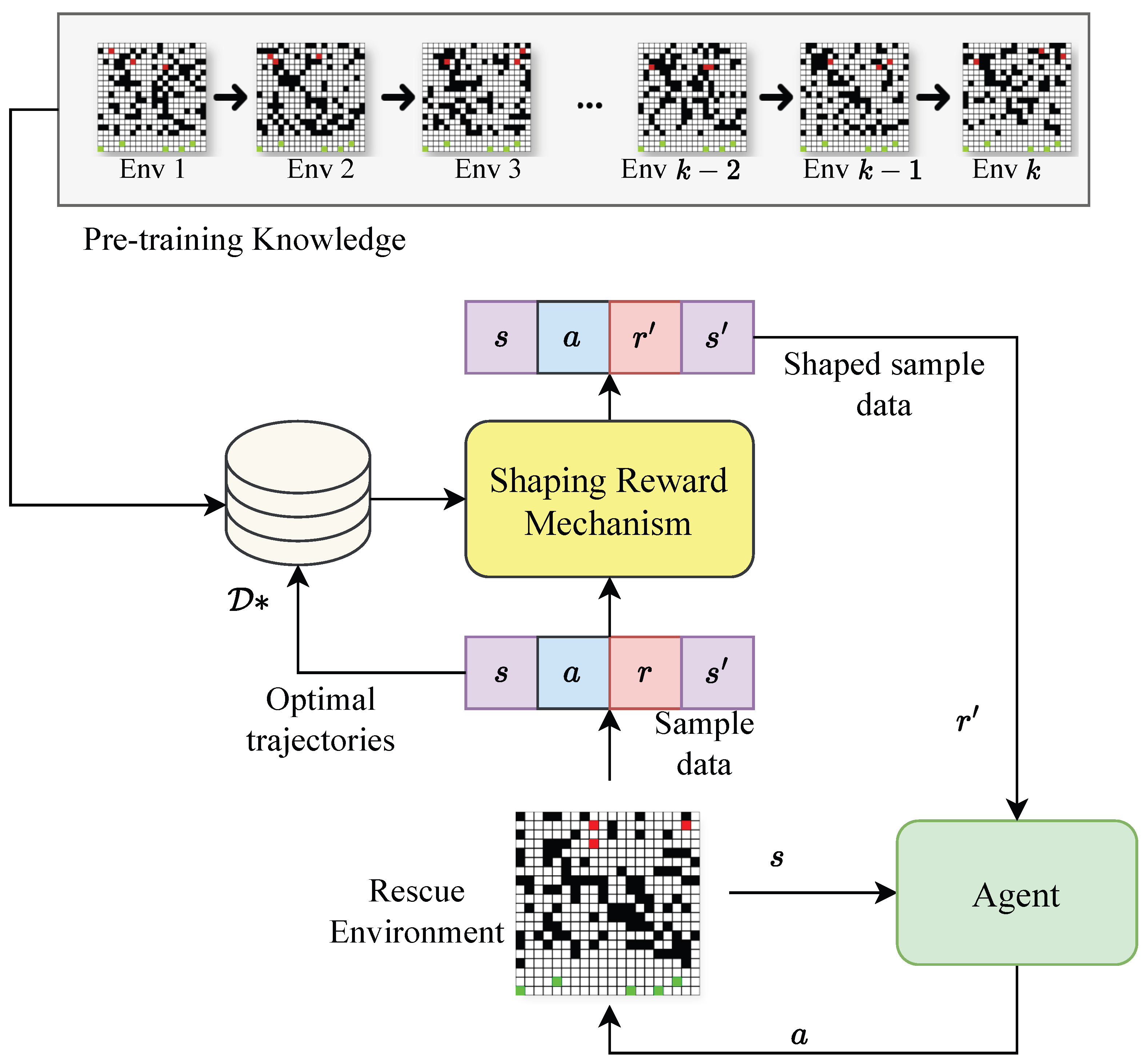
The proposed methodology is summarised in Figure 1. The approach consists of designing a control policy that allows the drone to reach people who need assistance in a rescue environment, e.g., a post-earthquake disaster scenario. Here, we cannot assume prior knowledge of the debris-covered area due to the damage caused by the earthquake, such that the environment is highly modified. In view of this, the proposed approach adopts a lifelong reinforcement concept that aims to use previous experiences obtained from pre-trained models under similar post-earthquake environments to design a shaping reward (SR) heuristic that adapts the reward to the unseen rescue environment.

The pre-training knowledge includes experiences in the form of tuples of state s, action a, reward r, and next state $s^{\prime }$ of the trajectories that achieve the best performance in a particular rescue environment. These trajectories are used to construct an SR heuristic that adapts the reward function to better generalise to unseen scenarios using any reinforcement learning method. In this paper, we will focus on tabular reinforcement learning methods.

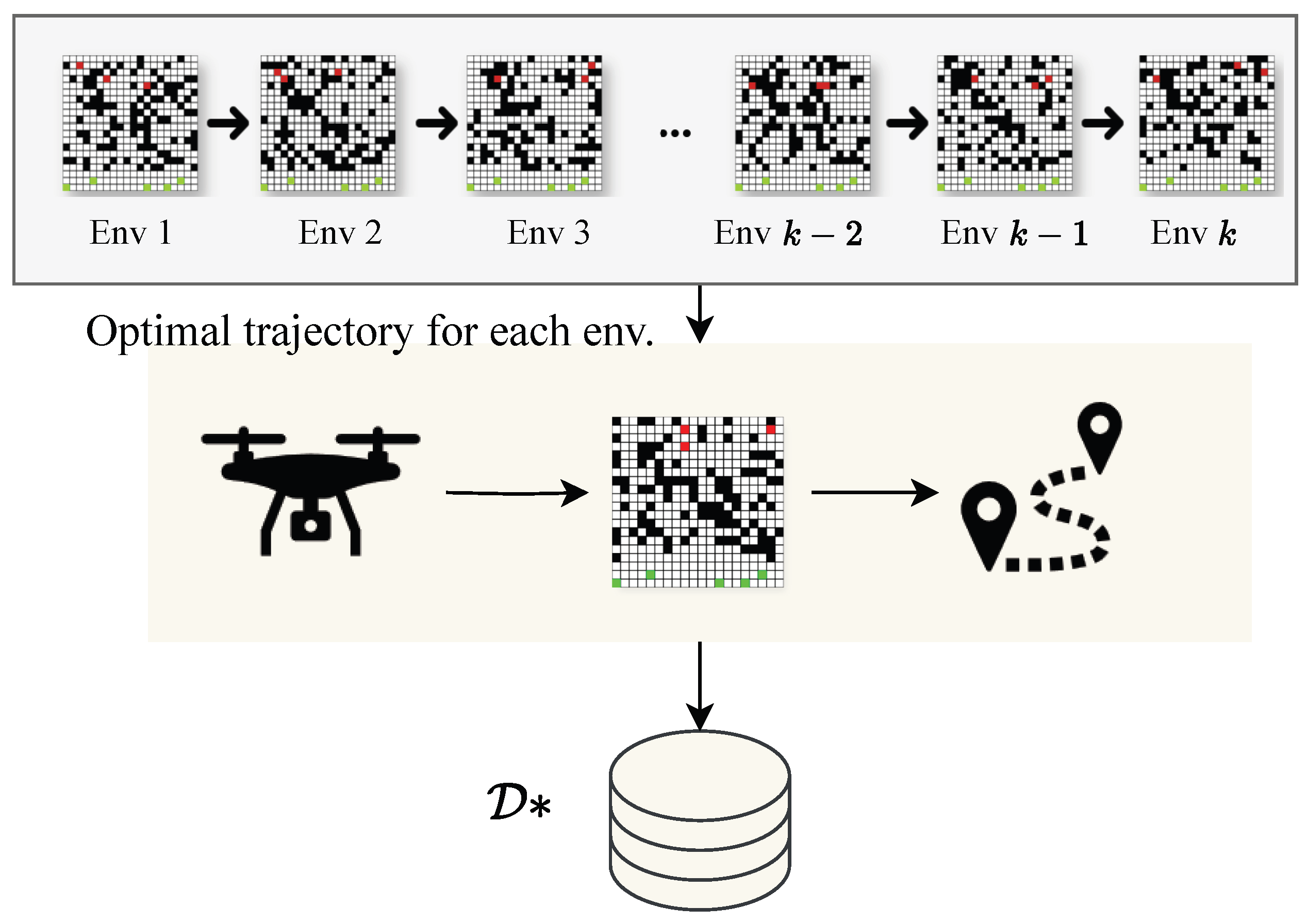
3.1. Shaping Reward (SR) Heuristic

The shaping reward (SR) heuristic consists of collecting the expert trajectories that give the best performance in a given rescue environment k as shown in Figure 2. This process is denoted as a pre-training stage.

In the pre-training stage, the optimal trajectories for each environment are stored and used to design an SR heuristic for future environments that guides the drone towards more efficient and effective decision-making.

To explain this process, we denote each trajectory data for an environment k as $T_k$ and it is represented by two components: (i) trajectory data ${\tau }_k^i$ composed by a the sequence of states and actions that the drone receives in each episode i with $i=1,\dots ,m$; (ii) the cumulative reward or return $G_k^i$ of the trajectory ${\tau }_k^i$ given by $G_k^i={\sum }_{j\ge 0}{r}_j$.

Here, we store only the trajectories of each environment that have the highest return since they provide more information on how the drone needs to behave in specific scenarios. So, for each environment k, we store the optimal trajectories and return denoted as ${\mathcal{D}}^{*}=\{{\tau }_k^{*},G_k^{*}\}$. Let us define $D\left(s\right)$ as the number of times that the state s appears in the dataset, and $D(s,a,s^{\prime })$ as the number of times a state transition $(s,a,s^{\prime })$ occurs in the optimal trajectory dataset ${\mathcal{D}}^{*}$.

Then, the SR heuristic is designed as

$$H(s,a,s^{\prime })=(1-\gamma )V_{max}\left({\displaystyle \frac{D(s,a,s^{\prime })}{D\left(s\right)}}\right),$$

(7)

where $V_{max}={\displaystyle \frac{R_{max}}{1-\gamma }}$ is a known upper bound of the value function in terms of the maximum value $R_{max}$ of the immediate reward $r_j$ in each step j of episode i. The heuristic $H(s,a,s^{\prime })$ is a non-potential based shaping function such that there exists a mapping $\Phi :S\times A\mapsto \mathbb{R}$, such that for all $s,s^{\prime }\in S$ and $a\in A$ the following is satisfied

$$H(s,a,s^{\prime })=\gamma \Phi (s^{\prime },a)-\Phi (s,a).$$

(8)

The incorporation of the SR heuristic can improve optimality of the Q-function. Here, tabular methods use either an off-policy or on-policy target which are, respectively, given by

$$\begin{array}{cc}\hfill Q^{*}(s,a)& =r(s,a,s^{\prime })+\gamma Q^{*}(s^{\prime },a^{\prime })\hfill \\ \hfill Q^{*}(s,a)& =r(s,a,s^{\prime })+\gamma \underset{u}{max}{Q}^{*}(s^{\prime },u).\hfill \end{array}$$

Consider the on-policy update rule which will be used for the Sarsa algorithm discussed in the next section. If we add the SR heuristic into the on-policy target and apply some simple algebraic manipulations, we give

$$\begin{array}{cc}\hfill Q^{*}(s,a)-\Phi (s,a)& =r(s,a,s^{\prime })+\gamma \Phi (s^{\prime },a)-\Phi (s,a)+\gamma \left(Q(s^{\prime },a^{\prime })-\Phi (s^{\prime },a)\right)\hfill \\ \hfill Q_{\Phi }^{*}(s,a)& =r_{new}(s,a,s^{\prime })+\gamma [Q^{*}(s^{\prime },a^{\prime })-\Phi (s^{\prime },a)],\hfill \end{array}$$

where $Q_{\Phi }^{*}(s,a)=Q^{*}(s,a)-\Phi (s,a)$ is the optimal Q-function moved by $\Phi (s,a)$ and $r_{new}(s,a,s^{\prime })=r(s,a,s^{\prime })+H(s,a,s^{\prime })$ is a new reward function. The term $\Phi (s^{\prime },a)$ adds a bias term into the update rule that adapts the Q-function based on the pre-training experiences. Notice that a greedy policy satisfies

$$\begin{array}{cc}\hfill a& {\displaystyle =arg\underset{u\in A}{max}{Q}_{\Phi }^{*}(s,u)}\hfill \\ \hfill & {\displaystyle =arg\underset{u\in A}{max}[Q^{*}(s,u)-\Phi (s,u)]}\hfill \end{array}$$

(9)

The above means that incorporating the SR heuristic modifies the optimality of the policy and it improves the Q-function to have better generalisation capabilities based on previous experiences collected in similar rescue environments. For the Q-learning target the same process can be applied to yield the same conclusion.

3.2. Reinforcement Learning Algorithm

In a rescue scenario, there is a need to reach the target goals as soon as possible such that the drone has to avoid spending too much time in exploring the environment. This means that the drone needs to be capable of recognising previously visited states and which actions were previously selected to accelerate the learning process and avoid long exploration phase. To this end, we will use a long short-term memory known as eligibility traces to enhance the capabilities of tabular methods.

Eligibility traces provide a unique skill to the RL algorithm, considering previously visited states and actions to accelerate learning and exploit more the acquired knowledge [40]. Two different algorithms based on eligibility traces are recognised: $Q\left(\lambda \right)$ and Sarsa $\left(\lambda \right)$, which are improved versions of both Q-learning and Sarsa algorithms [41] using eligibility traces, respectively. Here, we decide to focus mainly on Sarsa($\lambda )$ due to the nature of the rescue problem, which requires on-policy learning rather than off-policy for the proper action selection.

3.2.1. Sarsa $\left(\lambda \right)$ Algorithm

Sarsa $\left(\lambda \right)$ updates a Q-table based on an on-policy mechanism and the current temporal difference (TD) error as follows:

$$\begin{array}{cc}\hfill Q(s,a)& \leftarrow Q(s,a)+\alpha \underset{\mathrm{TD}-\mathrm{error}}{\underbrace{\left(r(s,a,s^{\prime })+\gamma Q(s^{\prime },a^{\prime })-Q(s,a)\right)}}e(s,a)\hfill \\ \hfill e(s,a)& \leftarrow \gamma \lambda e(s,a)+1_{(s_j=s,a_j=a)},\hfill \end{array}$$

(10)

where $a^{\prime }$ is the next action obtained by the selected policy or a GLIE (greedy in the limit with infinite exploration) policy, $\lambda \in [0,1]$ is the trace decay factor, and $e(s,a)$ denotes a specific kind of trace known as cumulative trace since it increases by 1 each time the drone is both at state $s_j=s$ with action $a_j=a$, otherwise it decays the trace by a factor of $\gamma \lambda$.

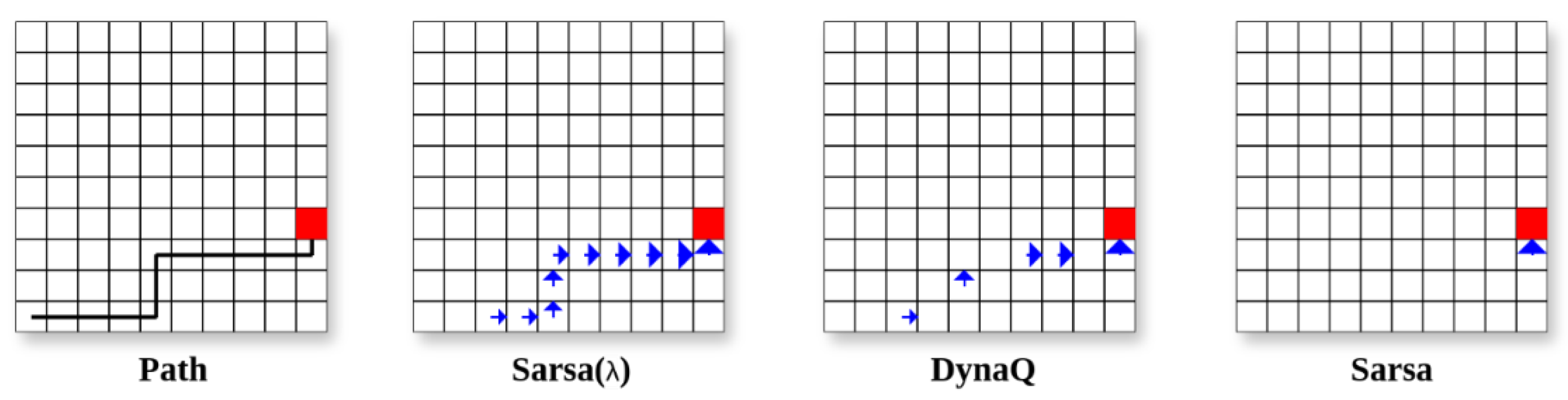
Figure 3 shows the magnitude of the TD-error at each state-action pair for a given path for the following tabular RL models (Sarsa, Dyna Q, and Sarsa $\left(\lambda \right)$).

The size of the arrows in the grids in Figure 3 represents the magnitude of the Q-function’s update error at each state-action pair. In all grids, the arrows indicate larger update errors along the path, reflecting substantial learning as the RL algorithm propagates the TD error throughout the trajectory. In the last three grids, representing different algorithms or stages of learning, the arrow sizes decrease, suggesting smaller updates as the respective Q-values approach convergence. This visual comparison highlights how Sarsa $\left(\lambda \right)$ efficiently spreads the learning signal across the state space, leading to faster and more effective convergence compared to traditional tabular RL algorithms. This clearly illustrates that the Sarsa $\left(\lambda \right)$ algorithm results in more comprehensive updates, particularly in early learning stages, ultimately enhancing the drone’s ability to generalise across different states.

3.2.2. Sarsa $\left(\lambda \right)$ with SR Heuristic: SR Sarsa $\left(\lambda \right)$

In this work, we enhance the generalisation capabilities of Sarsa $\left(\lambda \right)$ by introducing the SR heuristic into its design. This is conducted by simply injecting the new reward into the Sarsa $\left(\lambda \right)$ update rule as

$$\begin{array}{cc}\hfill Q(s,a)& \leftarrow Q(s,a)+\alpha \left(r_{new}(s,a,s^{\prime })+\gamma Q(s^{\prime },a^{\prime })-Q(s,a)\right)e(s,a)\hfill \\ \hfill e(s,a)& \leftarrow \gamma \lambda e(s,a)+1_{(s_j=s,a_j=a)},\hfill \end{array}$$

(11)

By leveraging eligibility traces and the SR heuristic, the drone’s generalisation capabilities are enhanced. In sparse environments such as rescue environments, when the drone samples terminal state positions, the Sarsa $\left(\lambda \right)$ algorithm propagates the one-step TD error across all $(s,a)$ pairs based on the trace $e(s,a)$. Compared to other tabular RL algorithms, eligibility traces accelerate the convergence of the Q-function, whilst the SR heuristic introduces generalisation capabilities to the RL algorithm for similar and unseen environments.

The combined Sarsa $\left(\lambda \right)$ with SR heuristic is denoted as SR Sarsa $\left(\lambda \right)$, whose pseudo-code is summarised in Algorithm 1.    

Algorithm 1: SR Sarsa $\left(\lambda \right)$ algorithm

Require: Optimal set of trajectories ${\mathcal{D}}^{*}$, initial Q-function and eligibility trace    $Q(s,a)=0$ and $e(s,a)=0$ for all $s,a$, learning rate $\alpha$, discount factor $\gamma$,         eligibility trace decay rate $\lambda$

1: for each episode i do

2:      Initialise the state s and reset $e(s,a)$ for all $s,a$

3:      for each step j do

4:           Select an action a using a greedy strategy, e.g., $ϵ$-greedy.

5:           Apply a and observe next state $s^{\prime }$ and reward $r(s,a,s^{\prime })$.

6:           Compute the SR heuristic $H(s,a,s^{\prime })$ using (7).

7:           Compute improved reward $r_{new}(s,a,s^{\prime })=r(s,a,s^{\prime })+H(s,a,s^{\prime })$

8:           Select the next action $a^{\prime }$ using a greedy strategy, e.g., $ϵ$-greedy.

9:           Update $Q(s,a)$ and $e(s,a)$ using the Sarsa $\left(\lambda \right)$ update rule (11).

10:         Set $s\leftarrow s^{\prime }$, and $a\leftarrow a^{\prime }$.

11:      end for

12: end for

4. Simulation Studies

In this section, we test and compare the proposed SR Sarsa $\left(\lambda \right)$ algorithm in a post-disaster earthquake scenario. As previously discussed, we focus on high-level drone navigation in a 2D maze-like environment, whilst the low-level controller is assumed to effectively drive the drone into the desired locations. In this environment, the positions of the patients, the obstacles, and the initial position of the drone are randomly generated. These settings mimic the real-world challenges of unknown casualty locations and navigating through intricate terrain. Three baseline algorithms enhanced with the SR heuristic are considered: SR Multi-step (MS) Sarsa, SR Dyna Q, and the state-of-the-art algorithm SR-LLRL based on the Q-learning algorithm [42].

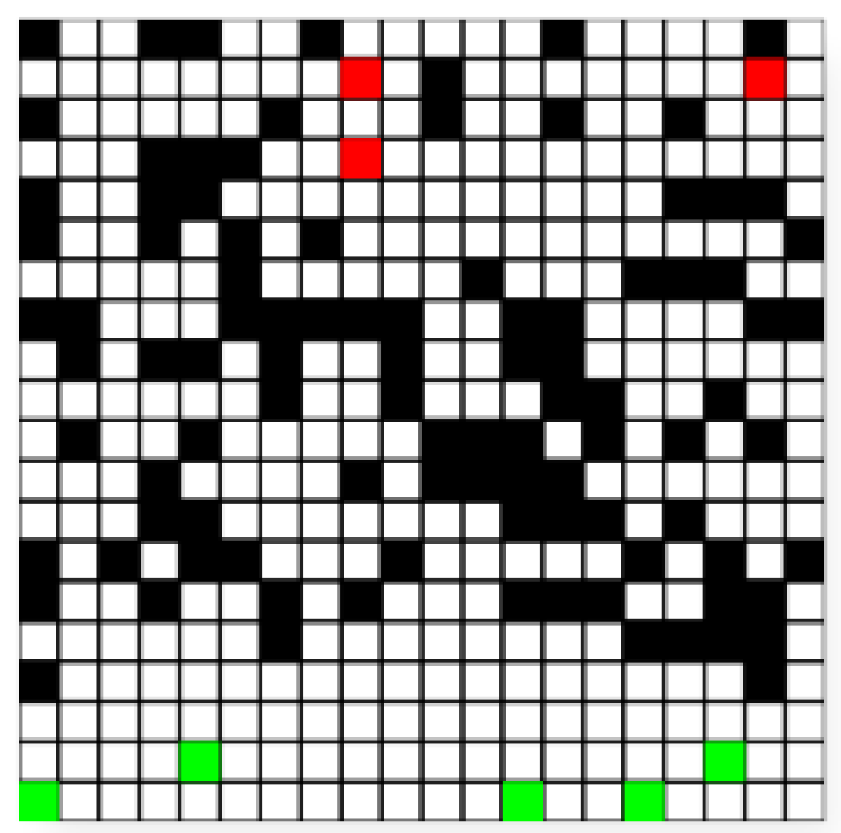
The rescue environment consists of a $20\times 20$ grid, which corresponds to 400 cells. We add 100 random obstacles to the environment. The grid has the following color specifications:

• Green grids: Consists of five grids where the drone may start. This emulates the fixed starting location of rescuers.
• Black grids: These grids represent the 100 obstacles generated in the environment.
• Red grids: These represent randomly generated patients, who are typically located far from the drone’s initial position, making them difficult to find.

We initiate drone operations from a safe standoff distance, allowing the platform to hover and observe the environment before entering complex or hazardous areas. The variability in each task comes from the different positions of obstacles, patients, and the drone’s starting point. After completing a task, the drone faces a new task and uses its prior knowledge to explore the new task and locate patients more quickly. Figure 4 shows a rescue environment sample.

A sparse reward function is designed manually and implemented in all the proposed models to ensure fair comparison. The reward is designed as follows: $+2$ for reaching each patient, and 0 for each step taken. For each environment configuration, the drone has 200 episodes and 200 steps to interact with it. After completing 200 steps, the drone is reset to the start state, and it starts exploring the task again. Each algorithm uses the following hyperparameter values: learning rate $\alpha =0.05$, exploration rate $ϵ=0.1$, discount factor $\gamma =0.9$, MS Sarsa steps $\mathrm{steps}=5$, and trace decay rate $\lambda =0.9$.

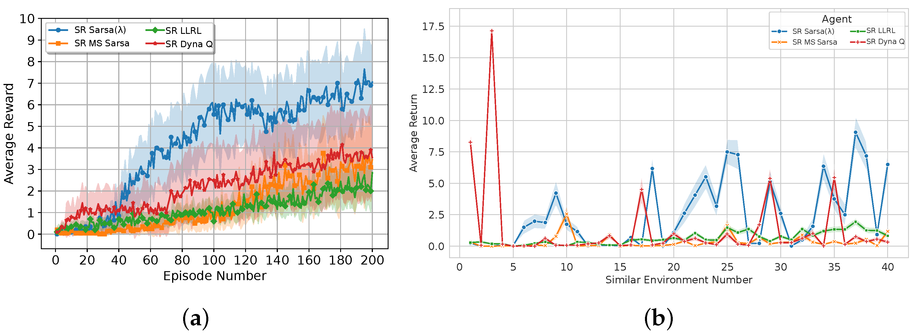
We evaluate the performance of each model based on two metrics: (1) the performance across episodes: each environment training consists of 200 episode, such that the score of the i-th episode is the average score across all the environments in the ith episode; (2) the performance across environments: each environment consists of 200 episodes, so the average score for the ith environment is the average across all 200 episodes for that specific environment. The results are shown in Figure 5.

The results show that SR Sarsa $\left(\lambda \right)$ outperforms the other algorithms due to its ability to update all state-action pairs efficiently through the use of eligibility traces. This comprehensive updating mechanism ensures that the drone quickly propagates reward information across the entire state space, leading to faster convergence and improved control policies. The average reward is almost twice as great as the second-best algorithm, SR Dyna Q. This highlights the robustness and effectiveness of SR Sarsa $\left(\lambda \right)$ in more complex scenarios, where its ability to efficiently propagate rewards across the state space becomes most beneficial.

SR Dyna Q is the second-best performer algorithm, primarily due to its model-based nature that allows for frequent updates through simulated experiences. This frequent updating enables SR Dyna Q to converge relatively quickly, although not as rapidly as SR Sarsa $\left(\lambda \right)$. SR MS Sarsa performs reasonably well due to its ability to incorporate more reward terms in the update rule, but it falls short compared with SR Dyna Q and SR Sarsa $\left(\lambda \right)$ due to its lack of memory.

Finally, SR LLRL performs the worst due to the one-step update of the Q-learning algorithm. This hinders the drone’s ability to adapt quickly, resulting in suboptimal policies, particularly in complex environments.

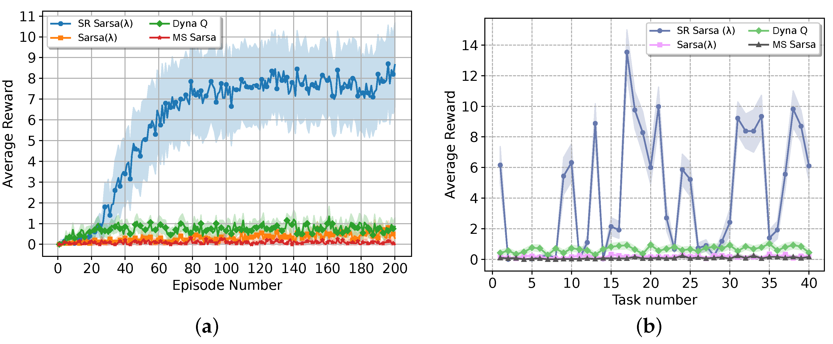
4.1. Impact of the Shaping Reward Heuristic

We compare the proposed SR Sarsa($\lambda )$ against non-lifelong reinforcement learning models to show how the SR heuristic enhances the overall performance of RL models. We compare the proposed approach against traditional tabular methods such as Dyna Q, Sarsa $\left(\lambda \right)$, and MS Sarsa. Figure 6 shows the comparison results.

The results highlight that none of the traditional tabular methods managed to reach a reward value of 1 across all episodes, whilst the SR Sarsa $\left(\lambda \right)$ outperform them with a reward of approximately 8.6. This shows the benefits of the proposed SR heuristic in the overall performance improvement of traditional RL methods. On the other hand, we can observe that the performance of the Sarsa $\left(\lambda \right)$ improves as the number of training environments increases, whilst the traditional models do not show a significant improvement. This difference highlights the critical impact of the pre-training phase in the SR Sarsa $\left(\lambda \right)$ algorithm, where the drone’s prior knowledge and experience allow for more efficient learning and adaptation to new tasks, leading to superior performance.

4.2. Ablation Studies

We perform ablation studies to verify the robustness of the proposed approach. To this end, we consider the robustness of the approach in the following scenarios: (i) different eligibility traces mechanism, i.e., either cumulative or replacing traces; (ii) changes in the number of obstacles (environment complexity); (iii) changes in the number of rescued individuals; and (iv) the pre-training strategy. Each ablation study is discussed as follows:

(i)

Eligibility traces update mechanism: We consider both cumulative and replacing traces to observe how the RL algorithms behave in a lifelong rescue scenario.

(ii)

Environment complexity: We consider five scenarios based on the number of obstacles. We consider 100, 80, 60, 40, and 20 obstacles, respectively. This study allows us to better understand how the complexity of the environment affects the overall performance of the approach.

(iii)

Number of rescued individuals: We vary the number of trapped individuals to assess the generalisation capabilities of the approach for multi-target problems.

(iv)

Pre-training strategy: We explore two different discovery strategies to identify the most efficient search strategy in a rescue scenario. We consider the following strategies:

• Breadth-first exploration: Where the drone has a small fixed number of steps to explore. If it is not successful, another drone begins the search from the initial position.
• Depth-first exploration: Where the drone has a larger number of steps to explore the environment without a reset.

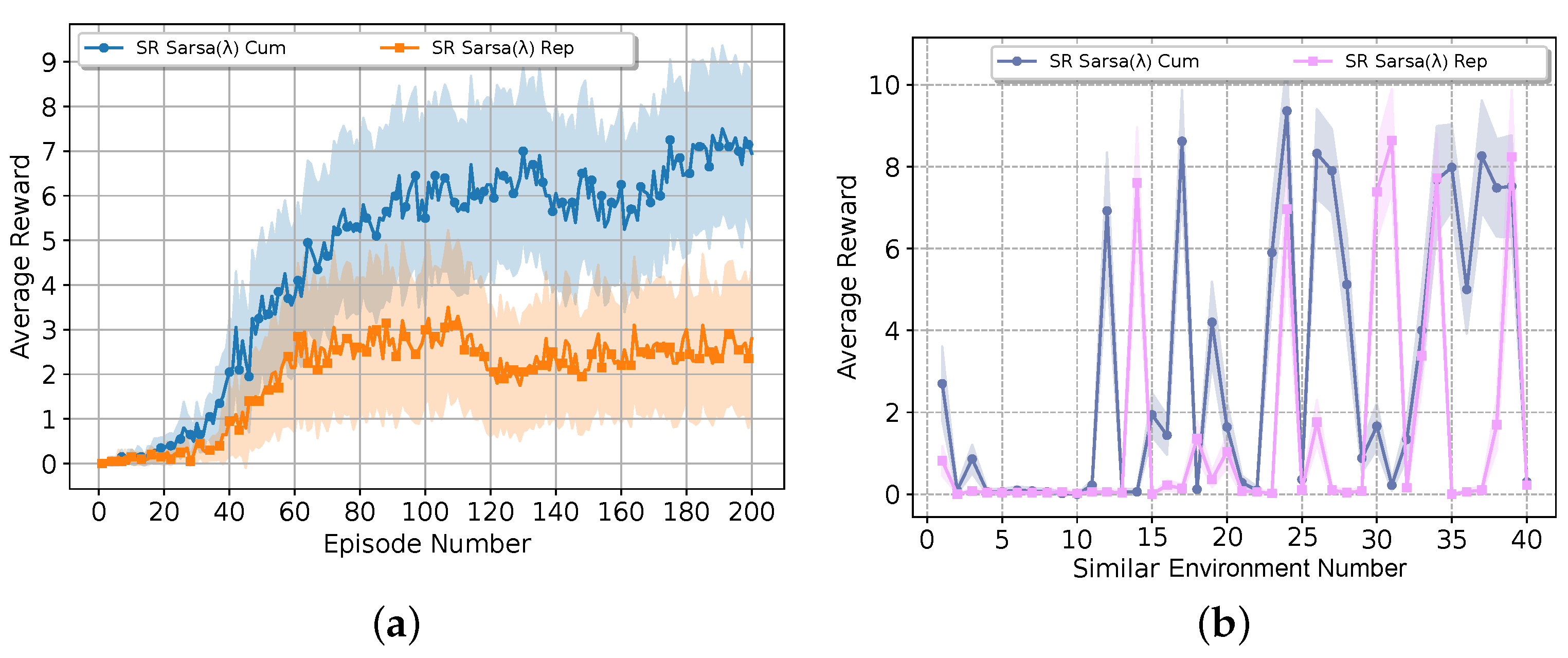
4.2.1. Cumulative Traces vs. Replacing Traces

We first analyse the update mechanism of the eligibility traces of the SR Sarsa $\left(\lambda \right)$. We consider two different updates: cumulative traces and replacing traces.

On the one hand, cumulative traces has the following update mechanism

$$e(s,a)\leftarrow \gamma \lambda e(s,a)+1.$$

(12)

Here, every time a state-action pair $(s,a)$ is visited, then the corresponding trace is incremented by 1, and the trace associated with non-visited states is decayed with a factor of $\gamma \lambda$. This method allows for the accumulation of traces over multiple visits, meaning that the more frequently a state-action pair is visited, the larger its trace becomes. This cumulative effect can lead to a stronger emphasis on frequently visited state-action pairs during learning.

On the other hand, replacing trace follows the following update rule:

$$e(s,a)\leftarrow 1.$$

(13)

In this case, whenever a state-action pair $(s,a)$ is visited, the trace is reset to 1, regardless of its previous state. This replacing method effectively limits the trace to a maximum value of 1, ensuring that recent visits have a stronger impact on learning, while older traces decay as usual according to $\gamma \lambda$.

The comparison experiments are designed to assess the convergence speed, stability of learning, and the overall performance of the drone. Key metrics included the number of episodes required to converge to an optimal control policy and the quality of the policies learned in terms of success rate.

Figure 7 shows the results of both updating mechanisms. The cumulative operator proved to be more effective in scenarios requiring long-term learning and consistent performance. It demonstrated the ability to recover from fluctuations and continued to improve over time, ultimately achieving a higher final reward. This makes the cumulative operator particularly well-suited for stable environments where sustained performance is crucial.

On the other hand, the replacing operator exhibits instability after a certain number of episodes. The reward drops, and it does not recover, which indicates that this update rule struggles to maintain consistent performance in the long term. However, its ability to quickly adapt to changes suggests that replacing traces could be more advantageous in dynamic environments where rapid responses are essential, even if this comes at the expense of stability.

The experimental findings suggest that while both traces have their strengths, the cumulative trace is generally preferable for tasks that demand robustness and consistent improvement. In contrast, the replacing traces might be better suited for scenarios where quick adaptation is prioritised.

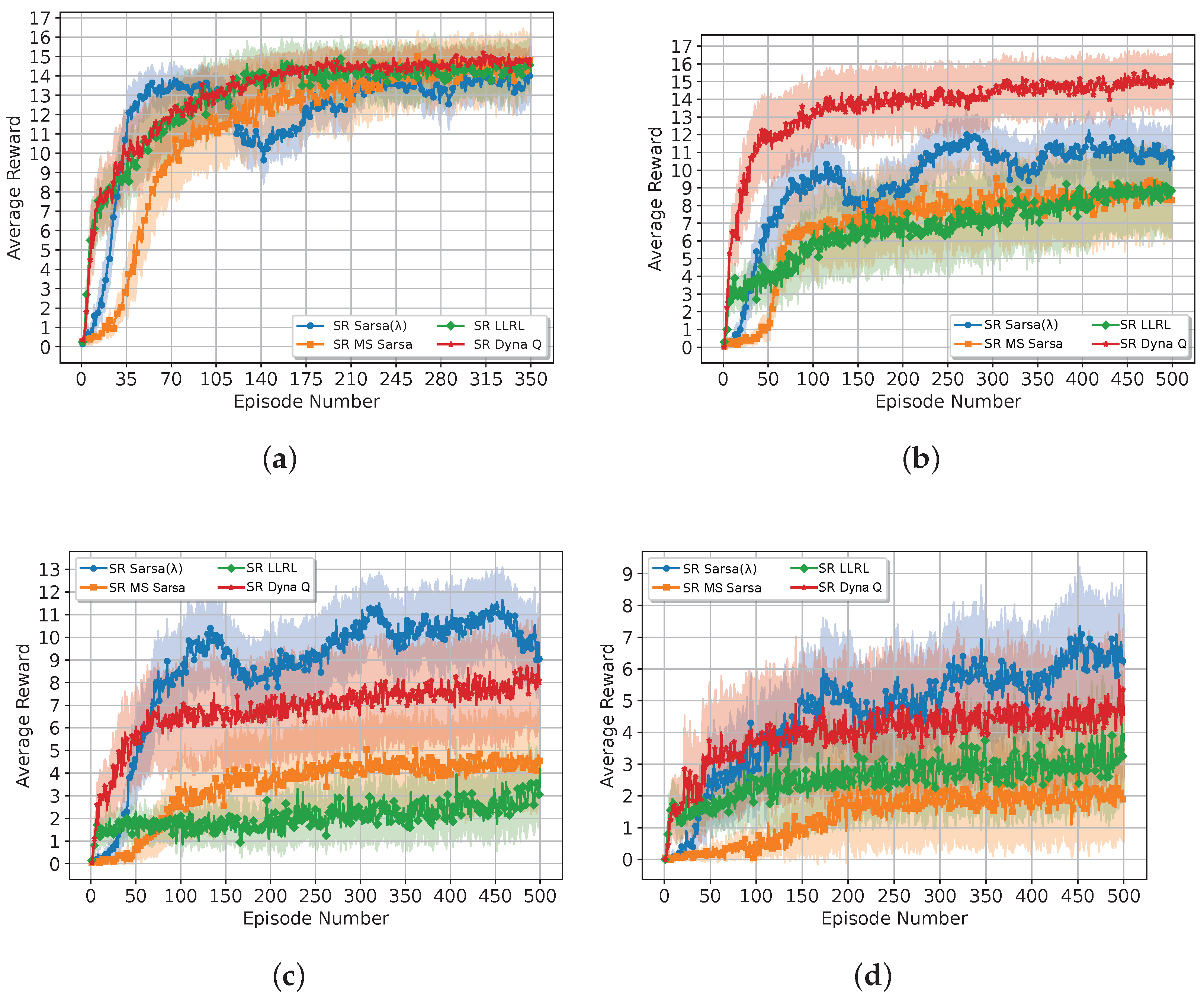
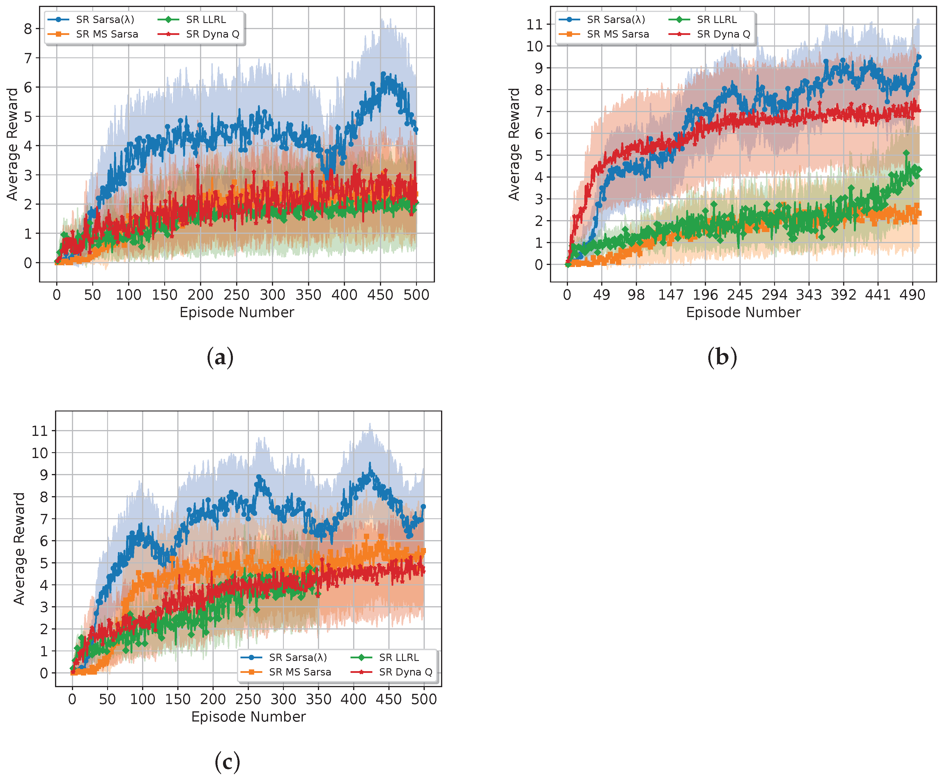
4.2.2. Impact of the Obstacle Complexity

Figure 8 and

Table 2. Ablation studies with different number of obstacles.

Number of Obstacles	SR Sarsa $(\mathit{\lambda })$	SR Dyna Q	SR MS Sarsa	SR LLRL
100	7.56	3.24	1.32	1.39
80	6.28	5.47	2.98	3.31
60	9.12	8.12	4.62	3.13
40	10.87	15.03	8.36	8.91
20	13.12	16.11	15.94	13.98

show the ablation studies results by varying the number of obstacles in the rescue environment.

The results highlight some interesting performance trends. On the one hand, the SR Sarsa $\left(\lambda \right)$ shows the best performance in the presence of environments with high complexity by leveraging the SR heuristic and the long short-term memory provided by the traces for efficient navigation. However, the efficiency of the SR Sarsa $\left(\lambda \right)$ slightly decreases for environments with low complexity. Here, the traces (depending on whether they are cumulative or replacing, which are discussed in future subsections) need to be explored more to cover all the state’s possibilities.

Conversely, the SR Dyna Q and SR LLRL show better results in environments with low complexity. Here, the off-policy nature of these algorithms helps to accelerate learning compared with the SR MS Sarsa. However, as the complexity of the environment increases, the drones experience a performance degradation, whilst the SR Sarsa $\left(\lambda \right)$ is consistent and improves its performance.

4.2.3. Impact of Trapped People Count

We assess the robustness of the proposed lifelong RL algorithms based on the number of trapped individuals or target goals, which play a critical factor that influences the overall performance of RL algorithm in rescue operations.

For this particular experiment, we consider a maximum number of three trapped individuals. The key goal of this study is to show the robustness of the algorithms to changes in the number of target goals in terms of efficiency (time) and success rate. Figure 9 and

Table 3. Average reward with different number of trapped people.

Trapped Count	SR Sarsa $(\mathit{\lambda })$	SR Dyna Q	SR MS Sarsa	SR LLRL
1	4.52	2.31	2.17	2.63
2	9.54	2.48	4.37	7.09
3	7.62	5.62	3.98	4.62

summarise the obtained results.

The results in Figure 9 show different performance patterns across all algorithms as the number of trapped individuals increases. We can observe that the SR Sarsa $\left(\lambda \right)$ becomes more efficient as the complexity increases due to its SR heuristic.

Notice that SR MS Sarsa and SR Dyna Q show an approximate linear increase in search time as the number of trapped people increases. SR Dyna Q struggles with the two-trapped-individuals case, where its performance drops before recovering slightly at the three-trapped-individuals case. SR Sarsa $\left(\lambda \right)$ demonstrates consistent performance across different trapped counts, showing the highest average rewards. The SR LLRL shows similar performances in all cases, showing that it struggles with the increase in the target patients.

4.2.4. Efficiency of Different Exploration Strategy

We compare the efficiency of the proposed approach under two different exploration strategies: (i) breadth-first and (ii) depth-first in a rescue task context. The rescue task involves searching for trapped patients in earthquake environments, where the patient’s location is unknown, and the environment is dynamic.

The experiments are conducted in dynamic earthquake environments, where the drone has to locate a varying number of trapped patients. The evaluation focused on two key metrics:

• Time required to find the first trapped patient: This metric reflects how quickly the drone can locate the first trapped individual in the environment.
• Total number of trapped patients found: This metric measures the overall effectiveness of the exploration strategy in finding all the trapped individuals.

The experimental results are shown in

Table 4. Depth-first exploration performance metrics.

Performance	Pre-Training Environment Number
	$\mathit{T}\mathbf{=}\mathbf{0}$	$\mathit{T}\mathbf{=}\mathbf{10}$	$\mathit{T}\mathbf{=}\mathbf{20}$	$\mathit{T}\mathbf{=}\mathbf{30}$	$\mathit{T}\mathbf{=}\mathbf{40}$
Steps required to rescue first patient	2751.3	2908.5	1562.5	1751.5	1251.7
Patient number found rate	0.90	0.97	0.97	1.0	1.0

and

Table 5. Breadth-first exploration performance metrics.

Performance	Pre-Training Environment Number
	$\mathit{T}\mathbf{=}\mathbf{0}$	$\mathit{T}\mathbf{=}\mathbf{10}$	$\mathit{T}\mathbf{=}\mathbf{20}$	$\mathit{T}\mathbf{=}\mathbf{30}$	$\mathit{T}\mathbf{=}\mathbf{40}$
Steps required to rescue first patient	7180.2	8195.5	13,560.5	6453.3	4830.9
Patient number found rate	0.63	0.67	0.60	0.73	0.67

. The results highlight specific differences in the performance of the breadth-first and depth-first exploration strategies when evaluated across varying levels of pre-training.

The breadth-first strategy generally excels in quickly locating the first trapped patient. For instance, without pre-training $(T=0)$, the time required to find the first patient is 7180.2 steps. However, with increased pre-training $(T=40)$, this time improves to 4830.9 steps. Despite this, the breadth-first strategy tends to cover a broader area more rapidly due to frequent resets, which mimics the effect of deploying multiple drones simultaneously. However, this approach leads to a lower overall number of patients found, with the patient number found hovering between 0.63 and 0.67, showing only modest improvement with pre-training. On the other hand, the depth-first strategy, though initially slower in locating the first patient (2751.3 steps at $T=0$), shows a significant reduction in time with pre-training, reaching 1251.7 steps at $T=40$. This method allows the drone to explore the environment more thoroughly without frequent resets, leading to more successful patient rescues. The number of patients found increases steadily with pre-training, reaching a perfect score of 1.0 at $T=30$ and $T=40$, demonstrating the effectiveness of the strategy in comprehensive search scenarios.

4.3. Dynamic Obstacles

We further test the proposed approach under dynamic obstacles. In this experiment, we fix the number of obstacles to 50. We conducted four experiments: (1) pre-training in dynamic environments and testing in different dynamic environments; (2) pre-training in dynamic environments and testing in static environments; (3) pre-training in static environments and testing in dynamic environments (depth-first); and (4) pre-training in static environments and testing in dynamic environments (breadth-first).

The results of these experiments are summarised in

Table 6. Pre-training in dynamic environments—testing in dynamic environments.

Performance	Pre-Training Environment Number
	$\mathit{T}\mathbf{=}\mathbf{0}$	$\mathit{T}\mathbf{=}\mathbf{10}$	$\mathit{T}\mathbf{=}\mathbf{20}$	$\mathit{T}\mathbf{=}\mathbf{30}$	$\mathit{T}\mathbf{=}\mathbf{40}$
Steps required to rescue first patient	917	1002.5	1018.3	878	1304
Patient number found rate	0.97	0.97	0.97	1.0	0.93

,

Table 7. Pre-training in dynamic environments—testing in static environments.

Performance	Pre-Training Environment Number
	$\mathit{T}\mathbf{=}\mathbf{0}$	$\mathit{T}\mathbf{=}\mathbf{10}$	$\mathit{T}\mathbf{=}\mathbf{20}$	$\mathit{T}\mathbf{=}\mathbf{30}$	$\mathit{T}\mathbf{=}\mathbf{40}$
Steps required to rescue first patient	2118.8	2295.0	2970.2	2468.8	2247.0
Patient number found rate	0.97	0.93	0.97	1.0	0.97

,

Table 8. Pre-training in static environments—testing in dynamic environments (depth-first).

Performance	Pre-Training Environment Number
	$\mathit{T}\mathbf{=}\mathbf{0}$	$\mathit{T}\mathbf{=}\mathbf{10}$	$\mathit{T}\mathbf{=}\mathbf{20}$	$\mathit{T}\mathbf{=}\mathbf{30}$	$\mathit{T}\mathbf{=}\mathbf{40}$
Steps required to rescue first patient	963.5	1214.1	975.5	818.5	874.9
Patient number found rate	1.0	0.93	0.97	1.0	0.97

and

Table 9. Pre-training in static environments—testing in dynamic environments (breadth-first).

Performance	Pre-Training Environment Number
	$\mathit{T}\mathbf{=}\mathbf{0}$	$\mathit{T}\mathbf{=}\mathbf{10}$	$\mathit{T}\mathbf{=}\mathbf{20}$	$\mathit{T}\mathbf{=}\mathbf{30}$	$\mathit{T}\mathbf{=}\mathbf{40}$
Steps required to rescue first patient	2966.5	1690.1	2358.3	2422.7	2413.1
Patient number found rate	1.0	0.90	0.93	0.97	0.97

. According to the time taken to find the first person in the four experiments, the efficiency of the SAR operation is improved slightly with the increase in pre-training tasks. However, pre-training in a dynamic environment can not significantly improve the model exploration efficiency with the increase in tasks.

The results show that the proposed SR Sarsa $\left(\lambda \right)$ can also improve dynamic efficiency in highly complex dynamic environments. Taking breadth-first as an example, drones pre-trained in static environments can also improve performance in more complex dynamic environments, which reflects the high generalisation of the proposed model.

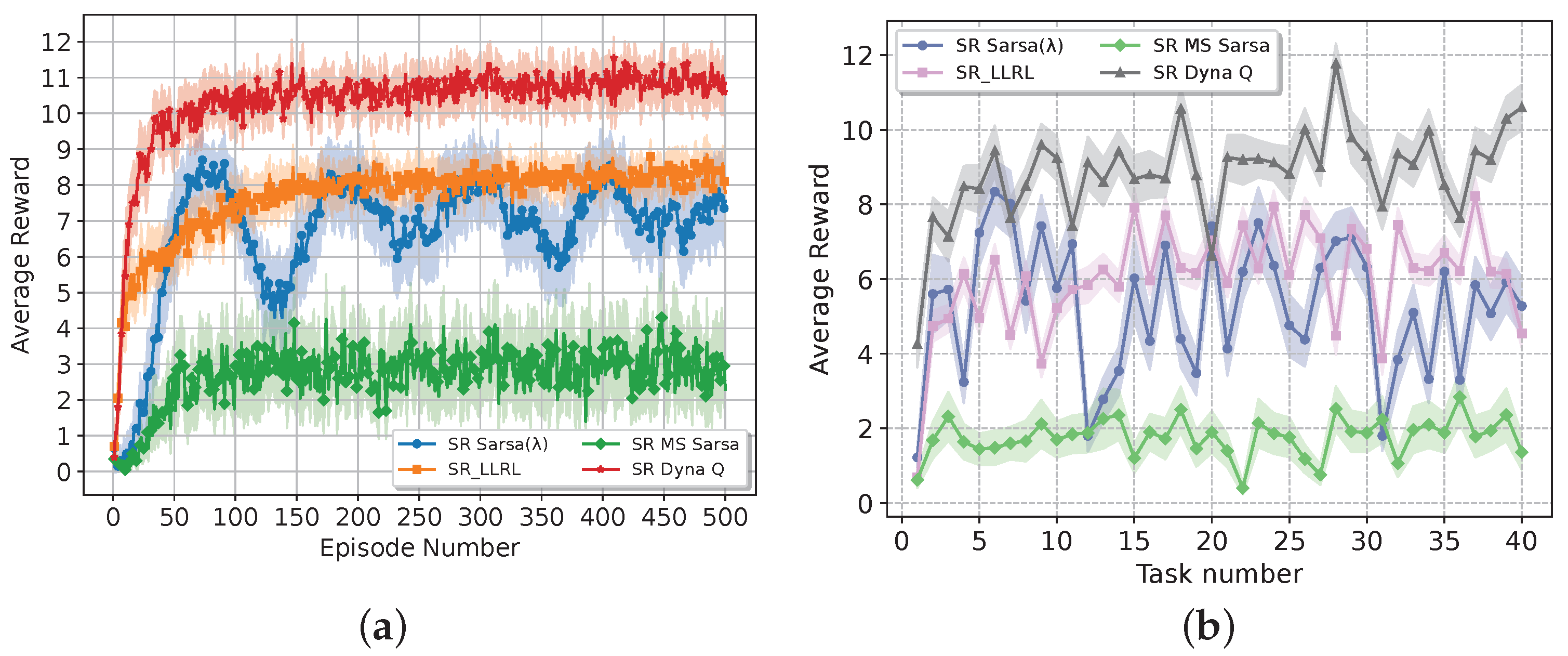
Figure 10 shows the comparison results of the proposed approach against other RL algorithms using 40 pre-trained dynamic environments. The results show that both SR Dyna Q and SR LLRL exhibit a better average return compared with the proposed SR Sarsa($\lambda$). This result is expected since the long short-term memory advantage of Sarsa($\lambda$) is lost due to the changes in the obstacles. However, the overall performance is still competitive.

4.4. Comparisons with Traditional Baseline Algorithms

The key non-RL algorithms used in the literature for SAR operations include PID controllers enhanced with Q-learning, Dijkstra, $A^{*}$, $D^{*}$, Rapidly-exploring Random Trees (RRT), and Artificial Potential Fields (APFs) algorithms (see Appendix A). Here, only the RRT and APFs algorithms comply with the assumptions of the proposed work, i.e., both the environment and the locations of the targets are unknown. Therefore, we only compare these algorithms against the proposed approach. To conduct fair comparisons, we used the following as metrics: (i) the number of steps needed to find the first patient and (ii) the patient’s coverage within 10,000 steps; both metrics in static and dynamic environments. The results are summarised in

Table 10. Comparison results against non-RL algorithms. Best results are in bold.

Environment	Metric	Algorithm
		RRT	APF	SR Sarsa $(\mathit{\lambda })$
Static	Steps to find the first patient	2621.0	10,000	1251.7
	Patients’ coverage	66.67%	0%	100%
Dynamic	Steps to find the first patient	842.0	10,000	818.5
	Patients’ coverage	100%	0%	100%

.

The results show that the RRT algorithm performs well in static and dynamic environments, such that it can effectively find the patients and adapt to environmental changes. In a static environment, it takes an average of 3000 to 6000 steps to find the first patient, and the average search and rescue coverage is about 70%. Conversely, the APF algorithm fails to find the patients and exhibits poor performance. This happens because the potential field does not explicitly use goal coordinates; instead, it relies on the combination of attractive forces towards unexplored regions and repulsive forces from obstacles. This limits the ability of the drone to target specific goal locations directly. The proposed SR Sarsa $\left(\lambda \right)$ in both static and dynamic environments outperforms the RRT algorithm in time and rescue coverage.

5. Conclusions

This paper proposes a lifelong reinforcement learning algorithm for rescue operations in post-earthquake disaster environments. The approach is based on a shaping reward heuristic that updates the reward function to generalise better to unseen environments. A Sarsa $\left(\lambda \right)$ algorithm is used as the main reinforcement learning algorithm to combine adaptation provided by the SR heuristic and long short-term memory given by the eligibility trace mechanism. A 2D maze-like rescue environment is designed which considers different numbers of obstacles and trapped people in different locations. The results of the simulation studies demonstrate that the proposed SR Sarsa $\left(\lambda \right)$ can successfully navigate and locate targets without prior knowledge of casualty locations. Additionally, the proposed method shows robustness across different environmental complexities and varying numbers of trapped individuals. According to the results from different exploration strategies, breadth-first search effectively covers most areas, making it easier to find more trapped people. The proposed approach is limited to discrete state-action spaces, which limits its generalisation to large or continuous state spaces. This can affect the performance of the shaping reward heuristic, which might require a different treatment. Additionally, a current limitation of the approach is that it assumes perfect low-level control tracking, neglecting sensor noise or uncertainties. These factors should be considered to increase the robustness and resilience of the approach. Future work will consider the implementation of the approach in a more realistic environment scenario to model other factors within the environment and drone sensing technologies, e.g., sensor noise, obstacles with different shapes, and 3D environments. In addition, the extension of the approach to deep reinforcement learning approaches with first responder feedback is a topic of our further work.