Unmanned Aerial Vehicle Anomaly Detection Based on Causality-Enhanced Graph Neural Networks

Abstract

With the widespread application of unmanned aerial vehicles (UAVs), the safety detection system of UAVs has created an urgent need for anomaly detection technology. As a direct representation of system health status, flight data contain critical status information, driving data-driven methods to gradually replace traditional dynamic modeling as the mainstream paradigm. The former effectively circumvent the problems of nonlinear coupling and parameter uncertainty in complex dynamic modeling. However, data-driven methods still face two major challenges: the scarcity of anomalous flight data and the difficulty in extracting strong spatio-temporal coupling among flight parameters. To address these challenges, we propose an unsupervised anomaly detection method based on the causality-enhanced graph neural network (CEG). CEG innovatively introduces a causality model among flight parameters, achieving targeted extraction of spatial features through a causality-enhanced graph attention mechanism. Furthermore, CEG incorporates a trend-decomposed temporal feature extraction module to capture temporal dependencies in high-dimensional flight data. A low-rank regularization training paradigm is designed for CEG, and a residual adaptive bidirectional smoothing strategy is employed to eliminate the influence of noise. Experimental results on the ALFA dataset demonstrate that CEG outperforms state-of-the-art methods in terms of Precision, Recall, and F1 score. The proposed method enables accurate and robust anomaly detection on a wide range of anomaly types such as engines, rudders, and ailerons, validating its effectiveness in handling the unique challenges of UAV anomaly detection.

1. Introduction

As a typical representative of new productive technologies, UAV technology has expanded its scope of application from the defense field (e.g., military reconnaissance and tactical strikes) to the civil field, including logistics, disaster rescue, and ecological monitoring. This expansion demonstrates significant market potential and practical value while driving a wave of innovation in the field of intelligent equipment [1,2,3]. However, the growing complexity of missions and the increasing harshness of operational environments have resulted in a notable rise in the failure rate of UAVs [4]. Additionally, due to cost limitations and constraints on system redundancy, there remains a substantial gap in reliability between UAVs and manned aircraft [5]. The dual challenges of safety assurance and mission reliability have made precision anomaly detection a critical technological frontier.

As UAV systems become increasingly complex, traditional model-based methods, such as parameter estimation, equivalent space methods, and state estimation [6,7,8,9], encounter bottlenecks including challenges in parameter identification and long validation cycles. Constructing high-fidelity physical or mathematical models for each type of UAV is highly complex, thereby restricting the applicability and effectiveness of model-based anomaly detection methods in practical scenarios. In contrast, data-driven methods avoid the time-consuming processes of parameter identification and model validation by directly extracting potential features from system operation data. Data-driven methods provide a more engineering-feasible technical path for UAV anomaly detection.

The practical implementation of data-driven methods heavily relies on multivariate time series data collected by the flight parameter recorder. Flight data comprehensively record the operating state parameters of UAV systems and the control quantities of actuators [10]. Given the limited availability of labeled anomaly data in flight data and the inherent unpredictability and variability of UAV anomalies, the UAV anomaly detection problem has increasingly been regarded as an unsupervised learning problem. In recent years, significant progress has been made in the development of various unsupervised learning methods, including autoregressive models [11,12], local outlier factorization (LOF) [13], clustering methods [14,15], one-class support vector machine (OC-SVM) [16], and support vector data description (SVDD) [17]. However, when applied to anomaly detection for high-dimensional and large-scale flight data, traditional unsupervised learning methods encounter challenges such as the curse of dimensionality and inefficient feature extraction. In this context, deep learning techniques have emerged as a promising alternative owing to their ability to perform automated feature mining through deep network architectures [18]. Among these, deep learning methods are of particular interest. Representative models include autoencoders (AEs) [19], generative adversarial networks (GANs) [20], long short-term memory networks (LSTM) [21], temporal convolutional networks (TCNs) [22] and their variants, etc. These methods extract intricate temporal patterns of flight data through different mechanisms.

Current research on deep learning-based UAV anomaly detection demonstrates a trend toward the integration of multiple technological approaches. Chen et al. [23] innovatively integrated the loss function of nonlinear support vector data description (SVDD) into an autoencoder framework. Focusing on UAV system characteristics, Yoo [24] developed a lightweight UAV anomaly detection system called MeNU, which achieves anomaly detection by encoding–storage–decoding. In terms of feature extraction, Yang et al. [25] utilized a 1D CNN-BiLSTM model as a feature extractor to improve the extraction of critical information from UAV flight data, guided by an attention mechanism. The CNN-SVM hybrid model introduced by Wang et al. [26] demonstrated the advantage of temporal feature extraction in real-time UAV status monitoring. However, while these methods perform well in temporal dynamic modeling, they are limited in their ability to comprehensively explore the correlations and interactions among complex high-dimensional flight parameters. UAVs are highly integrated intelligent complex systems. Flight parameters collected from various sensors and actuators are intercorrelated and interact with each other, and these correlations and interactions often critically influence the occurrence and propagation of anomalies.

Recently, graph neural networks (GNNs) have demonstrated significant effectiveness in modeling high-dimensional time series correlations [27], which have significantly enhanced the performance of anomaly detection by representing complex topological relationships between variables through a graph. Deng et al. [28] proposed an attention-based mechanism for a sensor feature embedding algorithm. He et al. [29] combined gated neural units and a graph attention model for UAV anomaly detection in order to establish topological dependencies among UAV sensors. Abro et al. [30] utilized a graph structure model based on the V-periodic algorithm, which calculates the deviation in the received signal strength indication data of each node from the average value and uses it as a feature in the graph. Wang et al. [31] designed an enhanced graph attention network incorporating a multi-head attention mechanism and a convolutional fusion transformer. This architecture effectively models long-term spatio-temporal dependencies, enabling the detection of anomalies through residual analysis.

However, these advanced GNN-based methods show obvious limitations when applied to the field of anomaly detection involving complex, multidimensional flight data. The main limitations are as follows: (1) the co-extraction of intrinsic temporal patterns and cross-dimensional spatial features under detection windows remains insufficiently resolved; (2) current architectures predominantly emphasize statistical correlations among flight data across dimensions while neglecting deeper causal relationships. These lead to inadequate accuracy and interpretability of state detection models, as well as reduced sensitivity to anomalies. In complex system analysis, causality and statistical correlation are fundamentally distinct [32]. The former reveals the irreversible physical mechanisms of action, whereas the latter merely reflects statistically significant dependencies between parameters. For instance, when a UAV executes a steering flight command, changes occur in the X-axis and Y-axis accelerations. In such cases, the UAV’s flight control system detects these acceleration changes and adjusts the yaw angle to correct the UAV’s heading. Here, the changes in X-axis and Y-axis accelerations serve as the cause, whereas the adjustment of the yaw angle represents the effect in response to these acceleration changes. This actual causality between flight parameters critically influences anomaly propagation. Therefore, incorporating parameter causality into anomaly detection models is essential for achieving more accurate, robust, and interpretable results. Furthermore, UAV flight data exhibit significant multi-source heterogeneity, comprising a mixture of continuous sensor data and actuator control signals. Sensor data typically manifest as high-sample-rate floating-point sequences, while control signals may represent low-frequency Boolean variables. Traditional loss functions may overlook weight differences between diverse data sources and struggle to capture their complex coupling relationships.

Driven by the above limitations and practical needs, we propose an anomaly detection model based on causality-enhanced graph neural networks. The model effectively detects anomalies in UAV flight data through multidimensional feature characterization and graph structure modeling. Specifically, the model establishes a two-stage feature characterization method: node features are jointly constituted by the intrinsic features of flight data and the temporal features of the trend decomposition, while edge features are characterized via matrix tensor fusion of causality and attention weights. The anomaly discrimination process is realized through iterative graph structure updates. The main contributions and advantages are summarized as follows:

• A spatio-temporal decoupled characterization method for flight data is proposed. This method leverages embedding vectors to represent the intrinsic features of each parameter and employs trend decomposition to extract temporal features from multidimensional flight data, thereby forming a joint characterization with decoupled spatio-temporal features.
• A two-stage causality identification method is designed to construct causality among flight parameters. It achieves directional enhancement of spatial features via a causality-enhanced graph attention mechanism, leverages graph neural networks to fuse spatio-temporal features, and realizes GNN aggregation and updates through multi-order neighborhood aggregation iterations.
• A low-rank regularization training paradigm is proposed. Additionally, an adaptive bidirectional smoothing strategy is adopted to eliminate the adverse effects of noise. Experimental validation demonstrates that our method achieves significant advantages on the ALFA dataset.

The rest of this paper is organized as follows: Section 2 provides an overview of related works. Section 3 details the proposed causality-enhanced graph neural networks. Section 4 presents the experimental results. Lastly, conclusions and directions for future research are discussed in Section 5.

2. Related Works

2.1. Flight Data Anomaly Detection

The classic definition of anomaly originates from statistician Douglas Hawkins’ seminal definition of an outlier: an outlier is an observation that deviates significantly from an established data distribution by a mechanism that may be distinct from the main data-generating process [33]. In the field of UAVs, flight anomalies are mainly manifested in two forms: (1) Instantaneous Anomalies, where sensor readings or actuator controls at a single point in time abruptly deviate from the normal range; (2) Flight-Level Anomalies, where multiple parameters within a specific flight phase persistently deviate from the normal operating range [34,35]. The essence of anomaly detection lies in recognizing observation patterns that deviate substantially from the expected or normal data distribution.

Anomaly detection can be formalized as a joint optimization problem of multivariate time series prediction and deviation analysis. Given multivariate flight data $X=\left[x^1,x^2,\dots ,x^T\right]$ over a time span of T, ${\widehat{x}}^{T+1}$ is the predicted value of the time series at time $T+1$ after the model is built, and $x^{T+1}$ is the true observed value at time $T+1$. An anomaly is detected if the following condition is satisfied:

$$∥x^{T+1}-{\widehat{x}}^{T+1}∥>\tau$$

(1)

$∥·∥$ is denoted as the deviation measure function, such as Mean Square Error (MSE) or Kullback–Leibler (KL) divergence. MSE represents the square of the difference, and KL divergence quantifies the dissimilarity between the predicted distribution and the true distribution by calculating the relative entropy. $\tau$ is a threshold determined based on confidence interval theory or extreme value analysis.

2.2. Graph Neural Networks

Graph neural networks (GNNs) represent a category of neural network models that have gained prominence in recent years. GNNs use graph structures as inputs to model topological relationships between data in non-Euclidean spaces, aiming to reason about data described by graphs. In GNNs, each node’s information is interconnected to neighboring nodes, and the information of each node can be updated through the aggregation of information from neighboring nodes. Graph Convolutional Networks (GCNs), which perform neighborhood feature aggregation through spectral domain convolution operations, effectively handle large-scale graph data. However, GCNs have limitations in capturing the varying importance of different neighboring nodes during feature aggregation. Building on this foundation, Graph Attention Networks (GATs) introduce an attention mechanism that dynamically assigns weighted contributions to neighboring nodes during feature aggregation, enabling nodes to stack layers of features with their neighbors in a more flexible manner. These developments have been employed in various time series modeling tasks, including traffic flow forecasting [36] and time series prediction [37]. Graphical Attention Networks facilitate more effective extraction of spatial features and exhibit superior performance compared to Graph Convolutional Networks in directed graphs [38]. In this paper, multivariate flight data are collected from sensors in different components or subsystems of the UAV, exhibiting significant spatial correlation across different dimensions. Consequently, GNNs can be employed to extract spatial features. The relationship among UAV flight parameters can be represented as a directed graph, with nodes corresponding to flight parameters and directed edges reflecting their relationships. However, existing methods often fail to fully consider the causality among flight parameters and the different degrees of importance of different parameters. Our proposed method aims to fill this gap.

2.3. Multivariate Time Series Causality Identification

Time series consist of a sequence of numerical values representing observations of a real-world variable, arranged in the order of their temporal occurrence. Such data are typically collected continuously by specific instrumentation, such as sensors, over a defined time period. The parameters of time series often exhibit complex correlations with unclear mutual influences. This is particularly evident in flight data, which are characterized by high dimensionality, strong coupling, and large volume, thus complicating the establishment of accurate models. Consequently, investigating how to effectively mine causality from time series has become a significant research topic. Granger initially introduced the Granger causality analysis method in 1969 for assessing the existence of interactions between bivariate time series. Since then, numerous improved models have emerged, which can be categorized into three main groups: methods based on regression analysis, information theory, and state space models [39,40]. However, methods based on regression analysis are limited to lower-dimensional time series, while methods based on state space models are restricted to binary systems. In contrast, methods based on information theory are extensively utilized for causality identification in high-dimensional time series data [40].

Based on information theory, Schreiber [41] proposed transfer entropy (TE) for evaluating the nonlinear causality between bivariate time series. TE quantifies the additional information that variable B contributes to variable A, given the complete historical information of variable A. Specifically, if the future state of variable A is entirely determined by its historical state, the transfer entropy value is zero. Subsequently, various causality analysis models, including biased transfer entropy, conditional entropy, and conditional mutual information, have been proposed. However, UAV flight data exhibit high dimensionality, strong coupling, and non-smoothness, making traditional methods susceptible to pseudo-correlation interference. In this paper, we propose a two-stage causality identification method that combines maximum mutual information coefficient (MIC) with transfer entropy to achieve causality identification in complex systems.

3. Proposed Method

3.1. Problem Definition

UAV flight data are multivariate time series obtained by sampling N flight parameters with time span T, $X=\left[x^1,x^2,\dots ,x^T\right]\in {\mathbb{R}}^{N\times T}$. According to the unsupervised anomaly detection method, the training set is composed only of normal flight data. The flight data on the training set are denoted as follows: $X_{train}=\left[x_{train}^1,x_{train}^2,\dots ,x_{train}^{T_{train}}\right]\in {\mathbb{R}}^{N\times T_{train}}$.

At time t, flight data $x_{train}^t\in {\mathbb{R}}^N$ constitute an N-dimensional vector representing the N parameter values of the recorded flight data.

The objective of anomaly detection is to detect anomalies in the test set, which is composed of the same N parameters. The test set is denoted as follows: $X_{test}=\left[x_{test}^1,x_{test}^2,\dots ,x_{test}^{T_{test}}\right]\in {\mathbb{R}}^{N\times T_{test}}$.

The output of the method is a sequence of $T_{test}$ binary labels, 0 for normal and 1 for abnormal.

3.2. Overview CEG

The proposed CEG method integrates temporal feature extraction with causality modeling through graph neural networks, aiming to capture causality and temporal features within high-dimensional flight data. By utilizing updates from causality-enhanced graph neural networks, it forecasts future variable results and detects anomalies by comparing predictions with actual observations. The overall structure is shown in Figure 1. It comprises the following five main components:

• Flight parameter causality identification: A two-stage causality identification method based on maximum information transfer entropy is utilized to construct a causal network among flight parameters;
• Causality-enhanced graph attention mechanism: Embedding vectors are employed to characterize the intrinsic features of flight parameters in each dimension. The causality-enhanced attention graph coefficient matrix is calculated based on the constructed causal network and the attention mechanism, achieving a causality-enhanced graph attention mechanism. The matrix elements can effectively quantify the strength of causality between different flight parameters;
• Temporal feature extraction considering trend decomposition: Data are subjected to a sliding window, and the temporal dependencies of the time series are captured through trend decomposition of the windowed data;
• Graph Aggregation: The causality coefficient matrix serves as edges in the graph, while time feature nodes and embedding vectors are integrated into the constructed graph as node features. Subsequently, node feature representations are updated by propagating and fusing information from neighboring nodes;
• Optimization and Anomaly Scores: The trained model predicts the next variable value and compares it with the observed value to compute an anomaly score. If the anomaly score exceeds the predefined threshold, the current data point is categorized to be an anomaly, thereby enabling effective anomaly detection.

3.3. Flight Parameter Causality Identification

In multivariate flight data, various variables can exhibit diverse attributes, and there exist complex causal relationships among them. Therefore, a flexible method is preferred to capture causality among flight parameters. We propose a two-stage causality modeling method based on maximum information transfer entropy. This method aims to reduce the impact of irrelevant parameters on modeling by leveraging a correlation network framework constructed using the MIC. Specifically, it reduces the computational burden of the transfer entropy component by filtering out weakly correlated relationships via a screening mechanism, and it only constructs a causal network between strongly correlated parameters.

Mutual information (MI) [42] is a fundamental metric in information theory used to quantify the reduction in uncertainty of one random variable as a result of knowing about another, indicating the degree of statistical dependence and the amount of information shared between the two variables.

Given input time series $X_{train}\in {\mathbb{R}}^{N\times T_{train}}$, for any two variables of time length $T_{train}$, $A=\left\{a_t\mid t=1,\dots ,T_{train}\right\}$ and $B=\left\{b_t\mid t=1,\dots ,T_{train}\right\}$, the value of MI between A and B can be calculated as follows:

$$MI(A,B)=\sum _{a\in A}\sum _{b\in B}p(a,b)log{\displaystyle \frac{p(a,b)}{p\left(a\right)p\left(b\right)}}$$

(2)

where $p(a,b)$ is the joint probability density of variables a and b, and $p\left(a\right)$ and $p\left(b\right)$ are the boundary probability densities of variables a and b. The probability density is calculated as follows:

$$p(a,b)={\displaystyle \frac{\mathrm{Number}\mathrm{of}\mathrm{data}\mathrm{points}\mathrm{in}\mathrm{grid}(a,b)}{\mathrm{Total}\mathrm{number}\mathrm{of}\mathrm{data}\mathrm{points}}}$$

(3)

Two variables are placed in a two-dimensional space, and a specific number of intervals are divided in the A and B directions, respectively. The distribution of scattered points in each grid is analyzed by observing the distribution of data points of A and B. The data points of A and B are divided by a network of $a\times b$. The joint probability is computed without requiring complex joint probability calculations, avoiding discretization bias and accurately capturing the correlation between variables.

The MIC is calculated as follows:

$$MIC(A,B)=\underset{a·b<B\left(T_{train}\right)}{max}{\displaystyle \frac{MI(A,B)}{{log}_{2}min(a,b)}}$$

(4)

where $B\left(T_{train}\right)$ is a parametric variable, representing the maximum number of the grid division. By systematically traversing the grid divisions, calculating the MI, and normalizing it, the maximum value of the normalized MI across all grids is defined as MIC, which signifies the maximum normalized mutual information value obtained from the feature matrix. Where $\omega \left(1\right)<B\left(T_{train}\right)<O\left(T_{train}^{1-\epsilon }\right)$, and $0<\epsilon <1$. $\omega \left(1\right)$ represents a constant and $O\left(T_{train}^{1-\epsilon }\right)$ represents the maximum value of $B\left(T_{train}\right)$. Generally, MIC performs optimally when $B\left(T_{train}\right)=T_{train}^{0.6}$. Upon calculation, the $MIC=\left(mi{c}_{ij}\right)$ values between N parameters yield the MIC matrix, and $mi{c}_{ij}$ quantifies the correlation between parameter i and parameter j, with values ranging between 0 and 1.

The universal applicability of MIC enables it to identify multiple types of correlation patterns with sufficient sample capacity, rather than being restricted to specific functional forms. The fairness of MIC ensures that different types of correlations can obtain statistically similar correlation coefficients under the same noise level. However, due to the symmetry of MIC, the correlation network constructed based on MIC cannot reflect the causal direction between variables. Transfer entropy can reveal the causal link between the driver and response variables without relying on an a priori model of the system. We calculate the causality of $mi{c}_{ij}>th$ to transform the nondirectional correlations into a unidirectional causality.

Before calculating the transfer entropy, the threshold $th$ is calculated by filtering the weakly correlated variables through the filtering factor $\gamma$. The filtering factor is set to the second significant digit of the unit of measure, and the filtering threshold $th$ is calculated as follows:

$$th=\left\{\begin{array}{cc}\left[{\displaystyle \frac{ave}{\gamma }}\right]\times \gamma \hfill & \mathrm{if}ave<1\hfill \\ \left[{\displaystyle \frac{ave\times \gamma }{\gamma }}\right]\hfill & \mathrm{if}ave>1\hfill \end{array}\right.$$

(5)

where $\gamma$ is the screening factor, $\left[·\right]$ is the rounding operation, and $ave$ is the mean of the nonzero $mi{c}_{ij}$. Further, the causality direction is determined by applying transfer entropy to the parameter pairs of $mi{c}_{ij}\ge th$, comprising the following:

For two time series of $A=\left\{a_t\mid t=1,\dots ,T_{train}\right\}$ and $B=\left\{b_t\mid t=1,\dots ,T_{train}\right\}$ with time span $T_{train}$, consider time series A and time series B. The transfer entropy is defined as follows:

$$T_{A\to B}=\sum _{b_{t+1},a_t,b_t}p(b_{t+1},a_t,b_t)log{\displaystyle \frac{p\left(b_{t+1}\right|a_t,b_t)}{p\left(b_{t+1}\right|b_t)}}$$

(6)

where $a_t$ and $b_t$ denote the historical observations of time series A and B, respectively, and $p(b_{t+1},a_t,b_t)$, $p\left(b_{t+1}\right|a_t,b_t)$, and $p\left(b_{t+1}\right|b_t)$ denote the joint probability density function and conditional probability density function, respectively. Determine the strength of causality based on the magnitude of transfer entropy. If $T_{A\to B}>T_{B\to A}$, the causality of $A\to B$ is determined, and $m_{ij}=1$. Conversely, if $T_{B\to A}>T_{A\to B}$, then B is the cause of A, and $m_{ji}=1$, where A and B are the ith and jth parameters, respectively. The causality value constitutes the causal matrix $M=\left(m_{ij}\right)$ of all parameters. The process of the flight parameter causality identification algorithm is shown in Algorithm 1.

The causal network provides a visual depiction of the causal matrix, as shown in Figure 2. In the network, the nodes correspond to the flight parameters, and the directed edges indicate the causality between these parameters. The values of the elements in the matrix correspond to the presence or absence of causality between the nodes in the network.

3.4. Causality-Enhanced Graph Attention Mechanism

For the flight data of $X_{train}$ or $X_{test}$, the dataset can be split into a series of subsequences through a sliding window. At time t, model input $x^{\left(t\right)}:=\left[\begin{array}{c}{x}^{t-\omega },x^{t-\omega +1},\dots ,x^{t-1}\end{array}\right]={\left[\begin{array}{c}{x}_1^{\left(t\right)},x_2^{\left(t\right)},\dots ,x_N^{\left(t\right)}\end{array}\right]}^T\in {\mathbb{R}}^{N\times \omega }$ is defined based on the historical data (either training or test set), when the window size is set to $\omega$. $x^{\left(t\right)}$ denotes the historical subsequence data with a time length of $\omega$, while $x_i^{\left(t\right)}$ denotes the historical subsequence data with a time length of $\omega$ in the ith dimension. Given the stride size $s_t$, the number of subsequences is as follows: $m=⌊{\displaystyle \frac{T-\omega }{s_t}}⌋+1$.

Algorithm 1: Causality identification.

Input: The training set $X_{train}$. Output: The causal matrix M. Initialize MIC as a new $N\times N$ matrix. for i = 1 to N do    for j = 1 to N do      if j == i then         ${\mathrm{mic}}_{ij}\leftarrow 0$      else         ${\mathrm{mic}}_{ij}\leftarrow \mathrm{MINE}(A,B).mic$    /* MIC */      end if    end for end for Initialize M as a new $N\times N$ matrix. for i = 1 to N do    for j = 1 to N do      if |micij| > th    /* Filtering threshold */ then         $(T_{ij},T_{ji})\leftarrow TE$    /* Transfer entropy */         if ${\mathrm{T}}_{ij}=0$ and ${\mathrm{T}}_{ji}=0$ then           ${\mathrm{m}}_{ij},m_{ji}\leftarrow 0$         else if ${\mathrm{T}}_{ij}-T_{ji}\ge 0$ then           ${\mathrm{m}}_{ij}\leftarrow 1$         else if ${\mathrm{T}}_{ij}-T_{ji}\ge 0$ then           ${\mathrm{m}}_{ji}\leftarrow 1$         end if      end if    end for end for return M

To effectively characterize the temporal attributes and intrinsic features of flight data, we introduce a multidimensional feature modeling method leveraging embedding vectors. By constructing a time-window observation model of time parameters, the system enables real-time feedback, performance evaluation, and parameter updating of the flight state. It is worth noting that, despite the dynamic and time-varying characteristics of the UAV flight state, the inherent causality among its parameters remains consistent. This consistency is primarily attributed to the fundamental physical principles governing UAV flight. Thus, we innovatively introduce learnable feature embedding vectors for each flight parameter, whose mathematical representations satisfy the following properties: the similarity in the embedding vectors can effectively reflect the similarity of the parameter behavior patterns, and the parameters with neighboring embedding representations exhibit significantly similar features.

Take a typical flight parameter as an example. Although pitch angle and altitude are collected by heterogeneous sensors, they exhibit an inherent coupling relationship at the dynamic level. Their flight data demonstrate significant temporal correlation. Similarly, flight data collected by homologous sensors may also exhibit potential behavioral similarities. This confirms the necessity of utilizing multidimensional embedded characterization: a microlearning mechanism to adaptively capture the heterogeneous nature of the parameters while preserving the capacity to uncover potential correlation patterns.

To capture the inherent properties of each parameter, we introduce an embedding vector as a representative feature: $v_i\in {\mathbb{R}}^d,i\in \left\{1,2,\dots ,N\right\}$, where d is the dimension of the embedding vector. We adopt a stochastic initialization strategy to generate parameter embedding vectors and jointly optimize parameter representations through end-to-end training. The embedding vectors serve two key functions: firstly, as node feature inputs in graph structure learning to guide the construction of graph structures; secondly, as heterogeneous influencing factors in the attention mechanism to achieve parameter feature fusion through adjustable attention weights. This dual application mechanism ensures that the model not only captures explicit parameter associations but also uncovers underlying heterogeneous interaction patterns.

A central goal of the model is to learn and characterize the causal strengths among parameters through graph structures. Based on the causal network created in Section 3.3, the causality-enhanced graph attention coefficient $\alpha$ between the nodes is calculated by applying the following equation:

$${\pi }_{ij}=\mathrm{ReLU}\left(a^T\left(\left(v_i\oplus W{x}_i^{\left(t\right)}\right)\oplus \left(v_j\oplus W{x}_j^{\left(t\right)}\right)\right)\right)$$

(7)

$${\alpha }_{i,j}={\displaystyle \frac{exp\left(\pi \right(i,j\left)\right)}{{\sum }_{k\in N\left(i\right)\cup \left\{i\right\}}exp\left(\pi (i,k)\right)}}$$

(8)

where $x_i^{\left(t\right)}\in {\mathbb{R}}^{\omega }$ is the input of node i, and $N\left(i\right)=\left\{j\mid m_{ij}>0\right\}$ is the set of cause parameters of node i obtained from the causal matrix. $W\in {\mathbb{R}}^{d\times \omega }$ is a trainable weight matrix, ⊕ denotes concatenation, and a is a vector of learning coefficients for the attention mechanism. The ReLU function is employed as the nonlinear activation to calculate the attention coefficients, followed by the application of the softmax function to normalize these values. In the causality-enhanced graph attention mechanism, edges represent the dependencies between parameters. These dependencies are not only closely associated with the causal relationships between parameters but also intricately linked to the causality-enhanced graph attention mechanism, which quantifies the influence weights of causality. The structure is represented by an adjacency matrix E, where the element ${\alpha }_{i,j}$ denotes the weight of the directed edge from node i to node j, representing the behavior of the jth parameter modeled using the ith parameter.

3.5. Temporal Feature Extraction Considering Trend Decomposition

Temporal feature extraction aims to capture dynamic temporal information in the time dimension. Ashish Vaswani et al. [43] introduced the Transformer architecture, which treats historical observations at each timestamp as a query vector. It computes the weighting of associated historical observations using the self-attention mechanism. This vector is subsequently utilized to predict future values. Although the Transformer enables parallel computation compared to traditional recurrent neural networks, its complex structure demands a large number of parameters. Additionally, its invariance to temporal order may lead to a loss of temporal information when processing time series [44]. Flight data exhibit unique time series characteristics, with each dataset covering distinct flight phases. The data characteristics and anomaly representations vary significantly across these phases, which can lead to biased anomaly analysis results if the entire process is treated as a uniform operating condition. In this paper, a simple trend decomposition method is employed to capture time series features.

The trend decomposition method is a combination of a positional coding strategy with a linear layer, where the raw flight data are decomposed into moving average components and phase trend components, i.e., $x_i^{\left(t\right)}=x_i^{s,\left(t\right)}+x_i^{p,\left(t\right)}$, moving average components $x_i^{s,\left(t\right)}=AvgPool\left(padding\left(x_i^{\left(t\right)}\right)\right)\in {\mathbb{R}}^{\omega }$, and phase trend components $x_i^{p,\left(t\right)}\in {\mathbb{R}}^{\omega }$. Two single linear layers are then applied to each component, and the two component features are summed to form the temporal features.

$$y_i^{s,\left(t\right)}=x_i^{s,\left(t\right)}{W}_i^{s,\left(t\right)}\in {\mathbb{R}}^d,W_i^{s,\left(t\right)}\in {\mathbb{R}}^{\omega \times d}$$

(9)

$$y_i^{p,\left(t\right)}=x_i^{p,\left(t\right)}{W}_i^{p,\left(t\right)}\in {\mathbb{R}}^d,W_i^{p,\left(t\right)}\in {\mathbb{R}}^{\omega \times d}$$

(10)

$$y_i^{\left(t\right)}=y_i^{s,\left(t\right)}+y_i^{p,\left(t\right)}$$

(11)

Since different phases of flight data have different characteristics, such as different moving averages and phase trends, they may assign different weights to different flight variables. Therefore, separate linear layers are constructed for each flight variable to extract features individually, and finally they are fused together to better capture the temporal patterns from the same flight variable.

3.6. Graph Aggregation

Graph aggregation aims to fully utilize the interdependencies among flight parameters across dimensions. After constructing the edges, a causality-enhanced graph neural network is employed to aggregate temporal features. Information from causality-related neighboring nodes is fused based on the learned graph structure. The constructed graph model forms the neighborhood matrix by using the calculated ${\alpha }_{i,j}$. The temporal features $y_i^{\left(t\right)}$ extracted in Section 3.5 are used as inputs to the graph neural networks. The aggregation and update of each node and its neighboring nodes are realized. Finally, the output of node i is obtained, representing $z_i^{\left(t\right)}$:

$$z_i^{\left(t\right)}=\mathrm{ReLU}\left({\alpha }_{i,i}W{y}_i^{\left(t\right)}+\sum _{j\in N\left(i\right)}{\alpha }_{i,j}W{y}_j^{\left(t\right)}\right)$$

(12)

where $y_i^{\left(t\right)}\in {\mathbb{R}}^d$ is the temporal characteristic of the node, and $W\in {\mathbb{R}}^{d\times d}$ is the shared linear transformation. From the graph aggregation process, all N nodes are represented as $\left\{z_1^{\left(t\right)},z_2^{\left(t\right)},\dots ,z_N^{\left(t\right)}\right\}$. Moreover, we also adopt LayerNorm, Feed-Forward, and residual connections in graph aggregation. Specifically, LayerNorm ensures stability and robustness, while residual connections enable information and gradients to flow more effectively in the network.

3.7. Optimization and Abnormal Scores

For each $z_i^{\left(t\right)}$, it is first multiplied by the corresponding embedding vector $v_i$, and the result $v_i\circ z_i^{\left(t\right)}$ is taken as the input to the fully connected layer to predict the flight data at time t.

$${\widehat{x}}^t=f_{\theta }\left(\left[v_1\circ z_1^{\left(t\right)},v_2\circ z_2^{\left(t\right)},\dots ,v_N\circ z_N^{\left(t\right)}\right]\right)$$

(13)

where “∘” denotes the Hadamard product or element-by-element multiplication of vectors, $f_{\theta }$ denotes the fully connected layer as a prediction function, and $\theta$ encompasses the layer’s parameters, including weights and biases. The output of the model is denoted as ${\widehat{x}}^t$, and MSE is utilized to minimize the discrepancy between the predicted output and the input data. To mitigate overfitting, a constraint term is added to the loss function, which is as follows:

$$L_{MSE}={\displaystyle \frac{1}{T-\omega }}\sum _{t=\omega +1}^{T_{train}}{∥{\widehat{x}}^t-x^t∥}_2^2$$

(14)

$$h\left(E\right)={\parallel E\parallel }_{*}=\sum _i{\sigma }_i\left(E\right)$$

(15)

$$L_{total}=L_{MSE}+\lambda h\left(E\right)$$

(16)

where E represents the matrix of attention coefficients for the graph structure, and ${\sigma }_i$ denotes the matrix singularity. To mitigate the risk of overfitting that may arise in the graph attention mechanism, a low-rank constraint is achieved by suppressing higher-order singular values, which motivates the attention mechanism to focus on key causality links that are consistent with system dynamics. A weight parameter $\lambda$ is introduced to balance the relationship between the error and the constraint term, which is appropriately determined by the performance of the validation set.

After obtaining the output for each time t, the next step is to detect anomalies that exhibit significant deviations from the expected normal patterns. First, the deviations on each parameter are calculated and then combined into isolated outliers for each timestamp. Since our model is built upon GNNs, the anomaly determination rules need to be designed specifically for the characteristics of this model. By comparing the predicted value ${\widehat{x}}_i^t$ with the corresponding observed value $x_i^t$, the difference is defined as $Err\left(t\right)$:

$$Err\left(t\right)={\displaystyle \frac{1}{N}}\sum _{i=1}^N\left|x_i^t-{\widehat{x}}_i^t\right|$$

(17)

Given the inherent complexity of UAV systems and the harsh operating environment, the collected flight data will inevitably be contaminated by noise, and data with high levels of noise may be mistaken for anomalies. The processing of the error sequence by using the moving average method can effectively reduce short-term noise fluctuations and filter out the pseudo-abnormal signals generated by transient disturbances while retaining the persistent abnormal characteristics. The Exponential Weighted Moving Average (EWMA) method is adopted to exponentially weight the current observed values and historical values, smoothing sequences with high noise or fluctuations. However, traditional EWMA may lead to backward bias along the time dimension; to avoid the temporal bias problem of traditional EWMA, an adaptive bidirectional smoothing strategy is designed to generate the smoothing scores $E_s\left(t\right)$.

Forward smoothing:

$$E_f\left(t\right)=\left\{\begin{array}{cc}Err\left(t\right),\hfill & t=1\hfill \\ \beta ·E_f(t-1)+(1-\beta )·\mathrm{Err}\left(t\right),\hfill & t\ge 2\hfill \end{array}\right.$$

(18)

Reverse smoothing: applying the same operation to the reverse sequence to obtain $E_r\left(t\right)$.

$E_f\left(t\right)$ is the error value for forward smoothing, $E_r\left(t\right)$ is the error value for backward smoothing, and $\beta$ is the initial weighting factor. It can be observed that the weighting factors can be updated adaptively as the moments change. The minimum error value $E_f\left(t\right)$ for forward smoothing and $E_r\left(t\right)$ for backward smoothing at moment t can be calculated as follows:  

$$E_s\left(t\right)=min\left(E_f\left(t\right),E_r\left(t\right)\right)$$

(19)

A time t is marked as an anomaly when $E_s\left(t\right)$ exceeds a predefined threshold. To avoid introducing additional hyperparameters, a simple method is used in the experiments to set the threshold to the maximum $E_s\left(t\right)$ of the validation set.

While various methods exist for determining the anomaly threshold, such as $3\sigma$ theory and the peak-over-threshold (POT) algorithm [45], $3\sigma$ theory is a method for detecting outliers based on normal distribution. POT is an extreme value theory that requires the assumption that the peaks in time series satisfy the Generalized Pareto Distribution (GPD). However, the applicability of the POT method may be compromised when the data peaks do not conform to the GPD assumption. Experimental results presented in the following section demonstrate that the proposed method offers better adaptability and performance. The process of the CEG-based model algorithm is shown in Algorithm 2.

Algorithm 2: Training and testing procedures of CEG.

Train Stage: Input: Training time series $X_{train}=\left[x_{train}^1,x_{train}^2,\dots ,x_{train}^{T_{train}}\right]\in {\mathbb{R}}^{N\times T_{train}}$, training epochs I, batch size D. Output: Optimized model parameter $W_{model}$. Randomly initialize parameter $W_{model}$ ($W_{model}$ includes all learnable parameters in CEG). for each epoch do    1. Apply the attention mechanism to the embedding vector and causal network to obtain the causality-enhanced graph attention coefficient.    2. Calculate the temporal feature.    3. Aggregate and update the graph neural networks to obtain an aggregated representation of the nodes.    4. Calculate the prediction value, minimize the loss function, and update the parameters in the neural network. end for return The optimized model parameter $W_{model}$. Test Stage: Input: Test time series $X_{test}=\left[x_{test}^1,x_{test}^2,\dots ,x_{test}^{T_{test}}\right]\in {\mathbb{R}}^{N\times T_{test}}$. for each $x^t$ do    1. Use the trained network to calculate ${\widehat{x}}^t$ and combine $x^t$ to calculate $E_s\left(t\right)$.    2. Obtain the predicted label by comparing the difference with the threshold. end for return Predicted label list.

4. Experimental Verification and Result Analysis

In this section, we present a comprehensive experimental evaluation of the proposed CEG. Firstly, we introduce a UAV dataset for anomaly detection. Next, we evaluate CEG on this dataset, demonstrating its superior or comparable performance to multiple baselines and significant outperformance over existing anomaly detection methods. Ablation studies are also conducted to evaluate the contribution of each key component, further demonstrating the effectiveness of the model components. Our proposed anomaly thresholds are very close to the theoretically optimal thresholds, exhibiting excellent accuracy.

4.1. Dataset and Performance Metrics

The experimental data used come from the flight data of the Air Laboratory Failure and Anomaly (ALFA) dataset. We briefly introduce the dataset in the following.

The AirLab Failure and Anomaly (ALFA) dataset [46], recently compiled by Carnegie Mellon University, is a valuable resource for investigating anomalies in UAV operations. The data were collected at the Pittsburgh airport using a modified Carbon Z T-28 UAV (e-Flite, Horizon Hobby, Champaign, IL, USA). In addition to the Pixhawk autopilot, the base platform has been augmented with a GPS module, an airspeed sensor for the airspeed tube, and an NVIDIA JetsonTX2 (NVIDIA, Santa Clara, CA, USA). The dataset encompasses processed data from 47 autonomous flights, featuring eight types of abrupt control surface failures, such as engine, rudder, aileron, and elevator failures. It includes 10 normal flights and 37 abnormal flights, with approximately 66 min of normal operation and around 13 min representing post-failure phases. Each flight is independently recorded with an associated timestamped anomaly detection log operating at a frequency of 5 Hz or higher. In addition, there is an additional feature called “Failure Status”, which indicates the timestamp when the failure occurred during the anomaly flight. In addition, one of the flight records has no ground truth information and is available for a total of 46 flights.

Table 1. Details of the ALFA dataset.

Anomaly Type	Test Cases	Before Anomaly (s)	After Anomaly (s)
Engine Failure	23	2282	362
Rudder Stuck to Left	1	60	9
Rudder Stuck to Right	2	107	32
Elevator Stuck at Zero	2	181	23
Left Aileron Stuck at Zero	3	228	183
Right Aileron Stuck at Zero	4	442	231
Both Ailerons Stuck at Zero	1	66	36
Rudder and Aileron at Zero	1	116	27
No Failure	10	558	-
Total	47	3935	777

shows the details of the dataset.

Each flight record contains information received using the MAVLink V2.0 node for the Robot Operating System (MAVROS), including GPS information, local and global status, and wind estimates. Most of the topics are inherited from the original unmodified MAVROS module, in addition to high-frequency data for measuring (via sensors) and commanding (via the autopilot) roll, pitch, speed, and yaw. For each maneuvering surface, the corresponding values become nonzero in the event of a failure.

The ALFA dataset, comprising raw flight logs, encompasses various data functionalities, including sensor readings and system status details. To enhance spatial data integration, the preprocessing step employed an intelligent transformation to serialize the data into cohesive planar tables. This process addressed potential data sparsity through smoothing, producing a complete and refined dataset composed of interpolated and smoothed values.

The ALFA-collected multivariate flight data included 350 parameters, with some being redundant and others being constant. To reduce input size, irrelevant and redundant parameters were excluded based on three criteria: (1) redundant and constant-type parameters; (2) derived parameters, such as covariance between parameters; and (3) insufficiently stable sensor parameters, such as changes in the logbook sources during the flight process.

Table 2. Selected flight parameters in ALFA dataset.

Parameter	Description
Orientation	The direction of the UAV, expressed as a quaternion, which consists of x, y, z, and w.
Angular velocity	Rate of change in angular velocity in the x, y, and z axes.
Linear acceleration	Acceleration values in the x, y, and z directions.
Mag	Components of the magnetic field measured along the x, y, and z axes.
Velocity	Velocity in x, y, and z directions.
Position	Spatial position of the UAV.
Airspeed	Airspeed indicated by the UAV.
Euler angle	Pitch, roll, and yaw angles.
Deviation	Deviation between the actual and desired altitude, airspeed, and trajectory.
Pressure	Atmospheric pressure for altitude calculation.
Throttle	Control device that controls engine power.
Temperature	A physical quantity measuring the degree of heat or cold.
Groundspeed	The speed of motion relative to the earth’s surface.
RC input	Input signals received from the remote control to control the motion and function of the UAV channel1 and channel2.
RC output	Output control signals to drive the actuators of UAV channel1 and channel2.

shows the 36 flight parameters selected from the ALFA dataset, including sensor data and actuator control quantities. To address the variations in sampling rates across the collected data, the selected parameters were uniformly resampled to a uniform frequency of 10 Hz. Subsequently, the sensor measurements were standardized by the Z-score normalization technique. In this paper, flight data captured prior to the occurrence of any anomaly were designated as normal, whereas data recorded following the onset of an anomaly were marked as abnormal. The transition of the “status” field from 0 to 1 indicates the moment when an anomaly was triggered during the flight.

Figure 3 illustrates significant changes in some of the flight parameters when a UAV engine failure occurs or when the rudder becomes stuck to the left, showing a strong correlation between these parameters and the UAV anomaly. The red dashed line marks the moment of engine failure, while the pink area indicates the flight time after the anomaly occurred. Specifically, the linear accelerations in the X- and Y-axes exhibit significant fluctuations after engine failure, especially after the red dashed line, indicating that the UAV’s speed in the X- and Y-axis directions becomes unstable after engine failure. Concurrently, the airspeed also shows significant changes with a sharp decrease, which is typically associated with a reduction or complete loss of engine thrust. Additionally, when the rudder becomes stuck to the left, certain parameters also change significantly after the failure. The acceleration characteristics show significant fluctuations after failure, especially after the red dashed line, with a significant increase in fluctuations, suggesting that the acceleration in these directions changed drastically after the rudder deviation. The abrupt acceleration changes similarly result in sharp velocity fluctuations, further demonstrating the UAV’s velocity instability following rudder deviation.

Similarly, certain parameters demonstrate notable variations during anomalies affecting the ailerons and elevators. These observable shifts suggest a strong correlation between these parameters and the occurrence of anomalies, making them valuable indicators for detecting abnormal conditions. Through the analysis of characteristics associated with four distinct types of UAV malfunctions, it is observed that engine failure primarily impacts airspeed and overall flight speed. Meanwhile, a rudder stuck to the left primarily influences angular velocity, linear acceleration, and velocity. As a result, the features presented in Table 2 are capable of capturing the system’s behavioral changes following an anomaly. These significant changes serve as critical signatures for anomaly detection, offering a solid foundation for the development and implementation of the detection methodology.

Due to the fact that multiple anomaly-related features may be interrelated and change concurrently during an anomalous event, displaying intricate multidimensional dynamic behavior, it is difficult to achieve accurate detection by using individual features or predefined thresholds. In the next section, we experiment with UAV anomaly detection algorithms using these anomaly features. Since our proposed CEG is an unsupervised method, only normal flight data are used for model training.

To evaluate the performance of the proposed method, we use three key metrics: Precision, Recall, and F1 score. Precision measures the proportion of correctly identified anomalies among all instances flagged as anomalous, while Recall quantifies the ratio of detected anomalies relative to the total number of actual anomalies. The F1 score provides a balanced assessment by combining both Precision and Recall into a single metric. They are defined as follows:

$$Prec={\displaystyle \frac{TP}{TP+FP}}$$

(20)

$$Rec={\displaystyle \frac{TP}{TP+FN}}$$

(21)

$$F1={\displaystyle \frac{2\times Prec\times Rec}{Prec+Rec}}$$

(22)

where $TP$ denotes the count of true positive predictions, $FN$ refers to the number of false negatives, $FP$ denotes the number of false positive samples, and $TN$ denotes true negatives, reflecting the number of normal samples accurately identified.

4.2. Experimental Setup

Our method and its variants are implemented using Pytorch version 2.5.1 and CUDA 12.4, and are trained and tested using an Intel (R) Core(TM) i7-14700HX @ 5.50 GHz (Intel, Santa Clara, CA, USA) and NVIDIA RTX 4070 GPU (NVIDIA, Santa Clara, CA, USA). The training phase is conducted using the ADAM optimizer, setting the learning rate to $1\times {10}^{-3}$ and the batch size to 64, with a total of 100 epochs for training and an early stop at a setting of 10. For all datasets, the embedding vector size is 12, the sliding window is empirically set to 25, and the stride size is set to 1. The model hyperparameter $\beta$ is selected by grid search to be 0.2. To enhance the model’s robustness against noise, a controlled amount of Gaussian noise is introduced into the flight data during training.

There are 46 autonomous flights; among them, 10 normal data samples are allocated to the training set. The remaining 36 flights form the test set. Within the training set, we further partition the data into training and validation subsets following an 80/20 split. Specifically, 80% of the training data are used for model learning, while the remaining 20% serve as the validation set to track performance and mitigate overfitting. To enhance training efficiency and model generalization, we employ multiple dataloaders during the training process.

To minimize randomness in the training phase to obtain reliable results, each sample is trained and tested ten times independently. The final performance metrics are based on the average over ten times.

4.3. Flight Parameter Causality Displays

Among the 36 flight parameters of the ALFA dataset, the two-stage causality identification method proposed in Section 3.3 is used for flight parameter causality identification. Different color nodes indicate the causal effects of parameters. The darker the color, the stronger the causal influence a node exerts on others, or the more strongly it is influenced by other nodes. Figure 4 illustrates the causality between the flight parameters. To simplify the representation, we visualize the partial causality of the partial parameters; specifically, multiple components describing the same parameter are simplified and merged into a single node to highlight the causality between the different parameters. The simplified graph structure is shown in Figure 5.

It is evident that identifying causality between parameters is meaningful. For instance, the causal chain from throttle to linear acceleration, then to velocity and position, is logical: an increase in throttle generates upward acceleration, which, when sustained, gradually alters the UAV’s velocity, thereby continuously changing its position. Angular velocity influences the Euler angle, which in turn affects acceleration. Specifically, UAV Euler angles (roll, pitch, and yaw) are derived from angular velocity integration around the three axes. Angular velocity describes the UAV’s rotational state, while Euler angles define its spatial orientation. The time derivative of the Euler angle equals angular velocity. Moreover, Euler angles influence thrust vectoring, leading to varying linear accelerations across axes. Additionally, atmospheric pressure indirectly reflects flight altitude, aiding state assessment. Based on the obtained causal network, the cause parameters corresponding to each flight parameter are obtained for the next calculation.

4.4. Experiments and Comparisons

4.4.1. Window Size and Step Size

In flight data anomaly detection, the sliding window method is used to segment data. The resulting subsequences are closely tied to the sliding window parameters, which directly impact the model’s feature extraction capability and computational efficiency. To determine an appropriate window size, we conducted window length parameter optimization experiments using eight typical configurations: 5, 10, 15, 20, 25, 30, 35, and 40 were selected for comparative study. The F1 scores are depicted in Figure 6. The results show that when the window length increases, the F1 scores show an increasing and then stabilizing trend. The model achieves the optimal F1 score when the window length is set to 25. This improvement can be attributed to the fact that longer windows incorporate more temporal data, enabling the model to more effectively learn long-term dependencies and identify underlying patterns or periodic behaviors in flight data. However, an excessive increase in the window length (e.g., 50) introduces redundancy, resulting in a significant increase in the computational cost and saturation of performance gain. In contrast, smaller windows (e.g., five) make it difficult to construct stable feature representations due to the lack of sufficient contextual information, thereby reducing the model’s generalization capability. Based on these findings, a window length of 25 is optimal.

Based on the optimal window length of 25, further experiments on sliding stride length parameter optimization are conducted, as shown in Figure 6. The results show that the detection accuracy shows a significant decreasing trend when the stride length is gradually increased from 1 to 8. This occurs because a larger stride size increases the distance the sliding window moves in each stride, reducing overlap between consecutive windows. While this accelerates training and prediction, the decreased number of samples limits the model’s capability to fully capture distribution information, thereby reducing its capacity to identify anomalous patterns. Although a larger stride size can shorten the training time, the loss of model performance outweighs the gain from computational efficiency improvement in this research scenario. Therefore, considering model accuracy and computational resource consumption, a sliding stride size of 1 is finally determined.

4.4.2. Baseline Comparison

To validate the superiority of the proposed method, we performed comparative experiments against several established unsupervised anomaly detection methods. These include deep learning-based models such as LSTM-VAE [47], MAD-GAN [20], OmniAno [48], GDN [28], Interfusion [49], and Anomaly Transformer [50]; density-based models such as LOF [13] and DAGMM [19]; and classical methods such as OC-SVM [16]. These methods are either based on reconstruction or prediction. Both our proposed method and other benchmark methods use the same optimizer, learning rate, batch size, window size, stride size, and epochs. For the unique parameters of each model, we set them to their own optimal hyperparameters.

• OC-SVM: The one-class support vector machine learns a boundary around normal data by projecting the data into a high-dimensional space. Anomalies are identified as data points outside this boundary;
• LOF: Local outlier factorization detects anomalies by evaluating the local density of a data point relative to its neighboring points;
• DAGMM: The deep autoencoding Gaussian model compresses input data into a low-dimensional latent representation through an autoencoder and models the distribution of the representation with the Gaussian mixture model. Anomalies are detected by examining the reconstruction error;
• LSTM-VAE: The LSTM-based variational autoencoder replaces the fully connected network with LSTM to capture temporal dependencies and models the data distribution through VAE;
• OmmiAno: OmniAnomaly adopts a stochastic recurrent neural network to model the normal patterns and uses the reconstruction probabilities to determine anomalies;
• MAD-GAN: Multivariate Anomaly Detection with Generative Adversarial Network employs LSTM-RNN for both the generator and discriminator roles within a GAN architecture, aiming to differentiate between normal and abnormal data effectively;
• GDN: The graph deviation network uses graph attention mechanisms to perform structure learning between variables and provides explainability for the detected anomalies;
• InterFusion: InterFusion employs a hierarchical variational autoencoder (VAE) to model normal patterns within multivariate time series data;
• Transformer: The Anomaly Transformer introduces a minimax strategy aimed at enhancing the distinguishability between normal and abnormal data by amplifying the discrepancy in their associations.

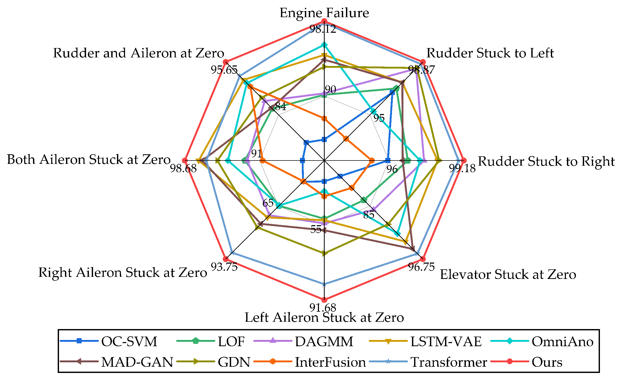
After ten rounds of experiments, the average Precision, Recall, and F1 score are evaluated on different types of anomalies. A performance comparison among different algorithms is shown in

Table 3. Performance comparison with existing methods in terms of Precision (%), Recall (%), and F1 score (%) on various types of anomalies. The best results are indicated in bold, while the second-best results are marked with an underline.

Method	Type of Anomaly
	Engine Failure			Rudder Stuck to Left			Rudder Stuck to Right			Elevator Stuck at Zero
	Pre	Rec	F1	Pre	Rec	F1	Pre	Rec	F1	Pre	Rec	F1
OC-SVM	80.68	90.44	85.28	95.39	97.49	96.43	96.96	94.71	95.82	76.85	80.14	78.46
LOF	86.79	93.73	90.13	97.26	96.27	96.76	98.36	95.10	96.70	81.36	86.24	83.73
DAGMM	89.32	91.29	90.29	98.04	98.62	98.33	98.26	96.59	97.42	81.76	90.42	85.87
LSTM-VAE	94.26	94.66	94.46	96.12	98.37	97.23	98.64	97.40	98.02	90.26	95.72	92.91
OmniAno	95.05	96.08	95.56	91.99	98.04	94.92	96.56	97.93	97.24	86.95	95.73	91.13
MAD-GAN	92.88	95.02	93.94	96.37	98.11	97.23	97.32	95.65	96.47	90.32	96.13	94.52
GDN	96.13	90.39	93.17	98.65	98.13	98.39	98.30	97.89	98.09	90.46	87.73	89.07
InterFusion	94.35	91.02	92.66	98.39	98.78	98.58	96.35	98.04	97.19	88.65	96.26	92.30
Transformer	97.96	97.90	97.93	98.65	98.75	98.70	99.12	98.78	98.95	92.32	98.99	95.54
Ours	98.03	98.21	98.12	98.24	99.51	98.87	99.63	98.74	99.18	94.56	99.04	96.75
	Left Aileron Stuck at Zero			Right Aileron Stuck at Zero			Both Aileron Stuck at Zero			Rudder and Aileron at Zero
	Pre	Rec	F1	Pre	Rec	F1	Pre	Rec	F1	Pre	Rec	F1
OC-SVM	19.82	68.66	30.76	39.56	57.52	46.88	76.35	99.20	86.29	71.25	82.19	76.33
LOF	39.23	68.89	49.99	56.29	67.63	61.44	86.89	98.54	92.35	81.29	87.91	84.47
DAGMM	43.55	65.51	52.32	56.64	82.63	67.21	88.24	96.34	92.11	80.96	92.35	86.28
LSTM-VAE	44.66	58.63	50.70	63.62	74.07	68.45	96.33	98.13	97.22	89.26	93.54	91.35
OmniAno	30.72	42.95	35.82	50.06	78.92	61.26	89.94	98.75	94.14	87.73	93.62	90.58
MAD-GAN	49.82	63.59	55.87	66.73	79.17	72.42	94.57	99.20	96.83	81.44	88.10	84.64
GDN	73.62	62.81	67.79	80.39	69.50	74.55	96.05	94.47	95.25	90.36	84.03	87.08
InterFusion	76.16	71.33	73.67	81.56	82.35	81.95	95.39	95.65	95.52	84.45	95.69	89.72
Transformer	73.47	96.97	83.60	83.04	97.88	89.85	94.92	97.97	96.42	87.62	97.45	92.27
Ours	88.94	94.59	91.68	88.51	99.65	93.75	97.97	99.40	98.68	92.36	99.18	95.65

. The proposed method achieves the highest F1 score on multiple types, demonstrating its superior balance between Precision and Recall. This balanced performance is particularly critical for effective UAV anomaly detection. In addition, our method exhibits the most satisfactory results on left- and right-aileron anomalies, which suggests that there is a low likelihood of generating false detections on these two error types.

Table 3 summarizes the comparison of Precision, Recall, and F1 score between CEG and the baselines across different anomaly types, with the best results shown in bold and the next-best results underlined. The results show that our model outperforms most of the baselines on each anomaly type. Specifically, on the entire dataset (i.e., the concatenated set of various anomaly types) versus the average of all the baselines (the average of the scores of the individual baseline methods on each anomaly type), the Precision of CEG improves by 10.60%, the Recall improves by 8.96%, and the F1 score improves by 10.25%.

It can be observed that most of the baseline methods perform better when anomalies occur in the engine and rudder because of their relatively simple anomaly patterns and spatio-temporal dynamics, and the F1 scores detected by CEG when anomalies occur in the engine and rudder are still better than those of the optimal baselines by 0.19% and 0.20%, respectively. In addition, most of the baselines perform poorly when the type of anomalies involves the left/right aileron stuck in the zero position, which may contain more complex anomalies. CEG achieves substantially better performance, improving the F1 score by at least 3.9% over existing methods. The integration of causality-enhanced graph attention with temporal modeling enables the network to effectively leverage both spatial and temporal dependencies within the flight data, allowing CEG to accurately capture the intricate spatio-temporal dynamics associated with these anomalies.

As expected, LOF, OC-SVM, and DAGMM exhibit inferior performance compared to most methods, possibly due to their limited ability to capture complex temporal patterns and insufficient modeling of spatio-temporal dependencies in flight data. In contrast, recent models such as GDN and Transformer-based methods demonstrate superior performance across multiple anomaly categories. However, GDN is less effective in obtaining temporal features from time series, and Transformer uses positional embedding, which can only see the local context window due to the inherent limitations of the Transformer architecture. Further analysis reveals the performance metrics on elevator anomaly types and finds that the proposed CEG algorithm outperforms other strong baselines. This performance gain is attributed to the effective integration of spatio-temporal characteristics in UAV flight data. By incorporating a causality-enhanced graph attention mechanism and trend decomposition method, CEG captures the interaction between different flight parameters and temporal information, effectively modeling the spatio-temporal correlation between flight data. The results show that this integration enables CEG to achieve higher prediction accuracy and recall in UAV anomaly detection. As shown in Figure 7, our proposed CEG achieves state-of-the-art performance on different anomaly types.

In addition, a sensitivity analysis of the parameter $\beta$ is performed for dispenser and elevator anomaly types, focusing on its effect on F1 score when $\beta$ takes different values.

Table 4. Hyperparameter analysis with F1 score (%) on two types of anomalies. The best result is indicated in bold.

Type of Anomaly	$\mathit{\beta }$
	0.1	0.2	0.3	0.4	0.5
Engine Failure	96.96	98.12	98.03	97.29	96.83
Elevator Stuck at Zero	95.27	96.75	96.65	96.44	96.40

reports the F1 scores as $\beta$ is incremented from 0.1 to 0.5 in steps of 0.1, and the results show that CEG is insensitive to $\beta$ and is robust to different hyperparameter settings.

4.4.3. Comparison of Ablation

To evaluate the contribution of each individual component of our method, we systematically remove different modules and record the performance changes. The experimental results of CEG and its variants on various anomaly types are shown in

Table 5. Results of ablation experiments of various types of anomalies in terms of F1 score (%). The best results are indicated in bold.

Ablation	Method	Engine Failure	Rudder Stuck to Left	Rudder Stuck to Right	Elevator Stuck at Zero	Left Aileron Stuck at Zero	Right Aileron Stuck at Zero	Both Aileron Stuck at Zero	Rudder and Aileron at Zero
Spatial characteristics	-Casual	94.13	98.19	98.36	90.73	72.48	78.82	95.34	91.56
	-Attention	95.62	95.33	96.52	93.83	73.75	79.44	96.66	93.23
	Pearson	89.82	93.37	93.25	91.59	68.62	85.18	92.45	87.23
	MIC	93.24	95.65	97.75	93.97	76.42	88.09	93.82	91.89
Time characteristics	-Temporal	94.18	97.72	97.68	92.83	78.86	84.37	96.38	92.21
	LSTM	96.94	98.03	98.35	94.62	86.25	88.32	97.26	93.32
	GRU	96.67	97.87	98.01	95.42	89.29	83.16	96.69	93.57
Loss function	MSE	97.14	98.31	98.26	94.39	87.25	91.66	97.39	93.72
	MAE	91.42	90.33	97.68	90.72	81.28	84.57	91.04	87.84
Ours		98.12	98.87	99.18	96.75	91.68	93.75	98.68	95.65

.

First, to assess the effectiveness and necessity of spatial feature extraction, we conducted ablation studies in which either the causality identification component or the attention mechanism was individually removed from the model. The results revealed that removing either component resulted in a significant performance degradation. The combined use of these mechanisms produced the most favorable results. Introducing the attention mechanism after causality identification enhanced the model’s adaptability. Causality defines each node’s neighborhood in the graph neural network, which is crucial for effective network aggregation and updating. Given the diverse properties of each univariate time series, the attention mechanism prevents uniform weight assignment across neighbors. Secondly, we further utilized correlation instead of causality for our analysis. The experimental results showed that our causality-based method significantly outperformed these correlation methods. This is primarily because Pearson and MIC study the correlation between parameters and cannot really capture the complex coupling between parameters. Thirdly, we removed the temporal feature extraction module to demonstrate its necessity and highlight the superiority of our method by comparing LSTM with GRU, which performed well in most cases through gating and long- and short-term memory mechanisms, but its ability to generalize UAV flight parameters based on the data appeared to be insufficient. As for the loss function, the loss function considering low-rank constraints improved the accuracy of the model more than a single Mean Square Error (MSE) or Mean Absolute Error (MAE). Our experiments consistently showed that removing any component of the proposed method led to performance degradation, thereby confirming the essential role of each individual part in the overall effectiveness of CEG.

4.4.4. Threshold Comparison

To evaluate how the threshold parameter $\tau$ influences anomaly detection performance, we analyzed its impact on the dataset’s F1 score, as shown in Figure 8. The results reveal a significant nonlinear relationship between threshold settings and model performance. Specifically, if the threshold is set too low, a rise in false detections will result in a sharp drop in Recall, which will result in a lower F1 score. If the threshold is too high, the false detection rate will increase, resulting in a decrease in Precision, similarly weakening the F1 score. Therefore, choosing an appropriate threshold is crucial for optimizing the F1 score.

The experimental results indicate that the adaptive bidirectional smoothing strategy achieves the highest performance (96.6%) compared to the $3\sigma$ criterion (88.9%) and the POT method (93.3%) across all test data types. Its threshold is also closer to the theoretically optimal value derived from grid search. Further analyses reveal that traditional methods are prone to fitness bias in non-stationary flight data due to strong assumptions on data distribution patterns (e.g., Gaussianity). In contrast, our proposed strategy mitigates distribution sensitivity by incorporating robust statistics through bidirectional smoothing, thereby achieving stable detection performance.

5. Conclusions

In this paper, we introduce a novel anomaly detection method for UAV flight data based on CEG. Specifically, the method constructs a graph structural model, which characterizes the intrinsic features and temporal features of each parameter through nodes. Edges are used to characterize the causality and attentional weights between parameters. These components are then fused using graph neural networks to effectively integrate temporal and spatial features. Furthermore, we propose a training paradigm with low-rank regularization adapted to the network structure and an adaptive bidirectional smoothing strategy.

To evaluate the advantages and performance of the proposed method, we conducted experiments on multiple anomaly types on the ALFA dataset. Compared to several state-of-the-art anomaly detection methods, our method demonstrates superior performance across Precision, Recall, and F1 score. The ablation study further confirms the contribution of each model component to the overall performance. In comparison to commonly employed threshold determination techniques, the anomaly threshold introduced in this paper demonstrates enhanced accuracy and approximates the theoretically optimal threshold more closely.

Despite this paper’s contributions to the technical field, certain limitations remain that require further investigation. Future research will focus on validating the proposed method across additional datasets and investigating hybrid strategies to enhance performance. These efforts aim to address key issues regarding the performance stability of different data distributions and their potential sensitivity to changes in training data.