

Drone-Based VNIR–SWIR Hyperspectral Imaging for Environmental Monitoring of a Uranium Legacy Mine Site

 , ,
, ,  , ,
, ,
Abstract
1. Introduction
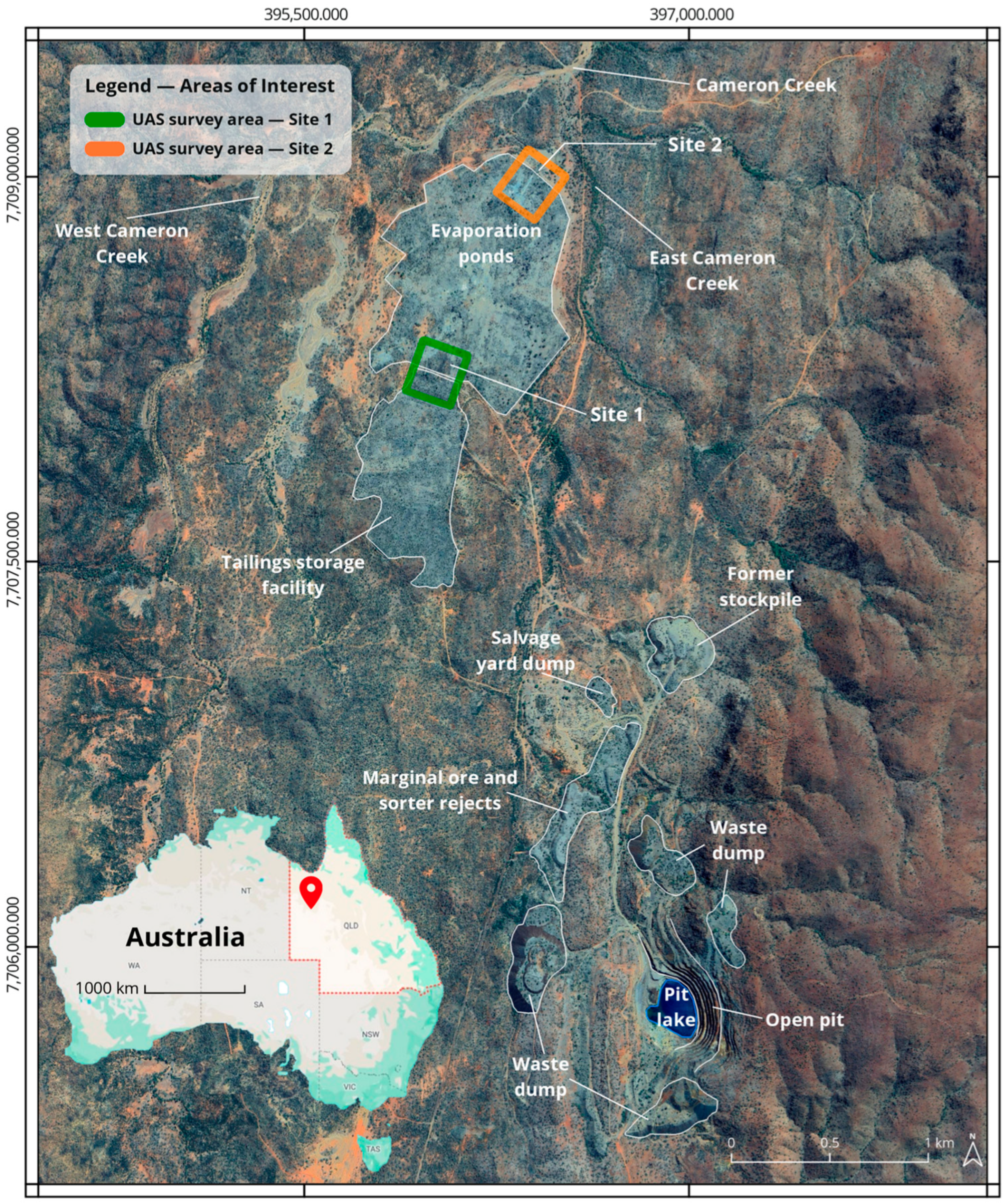
2. Study Site Background and Context
3. Materials and Methods
4. Results
4.1. Mapping and Masking of Vegetation Covers
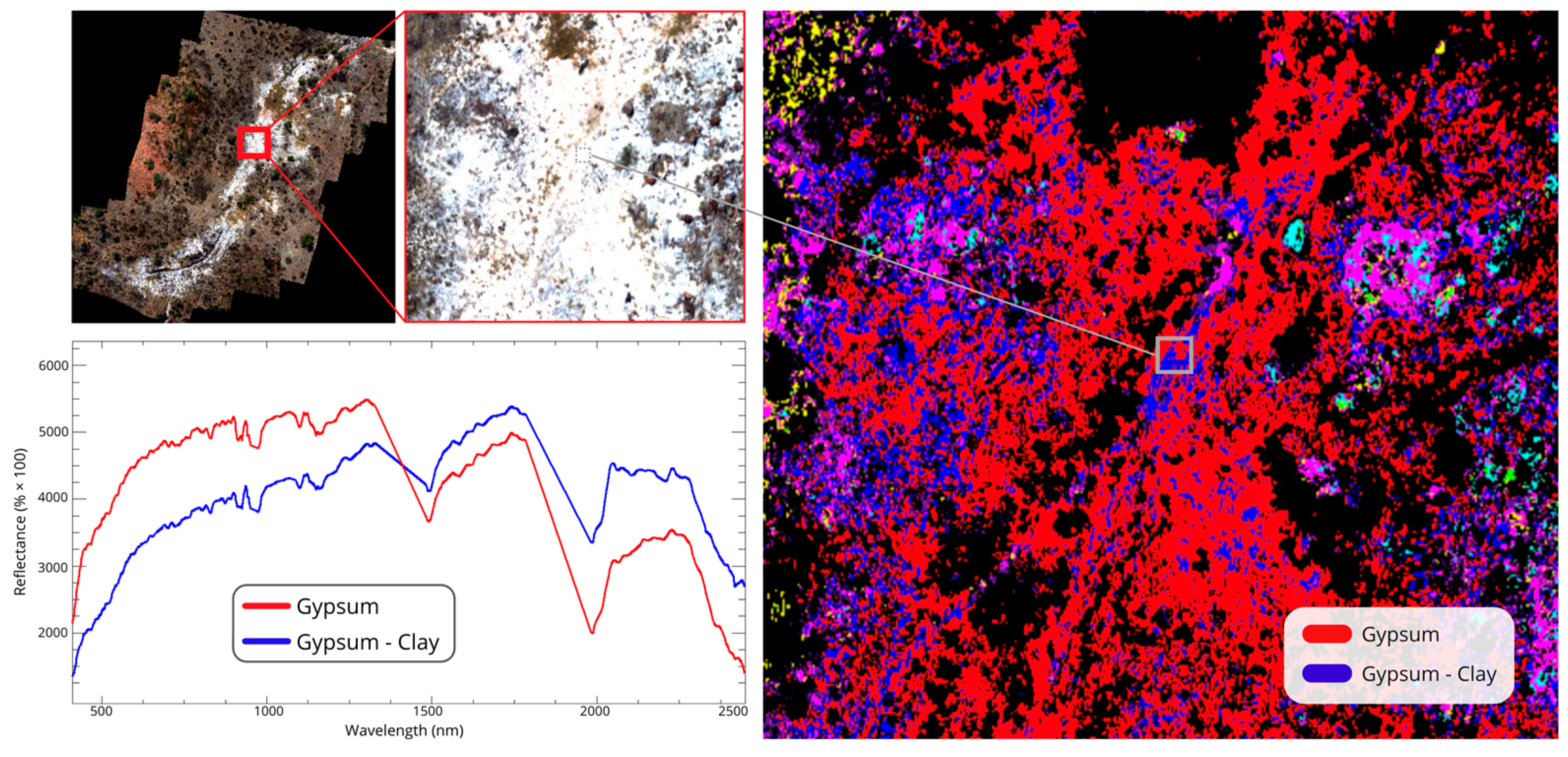
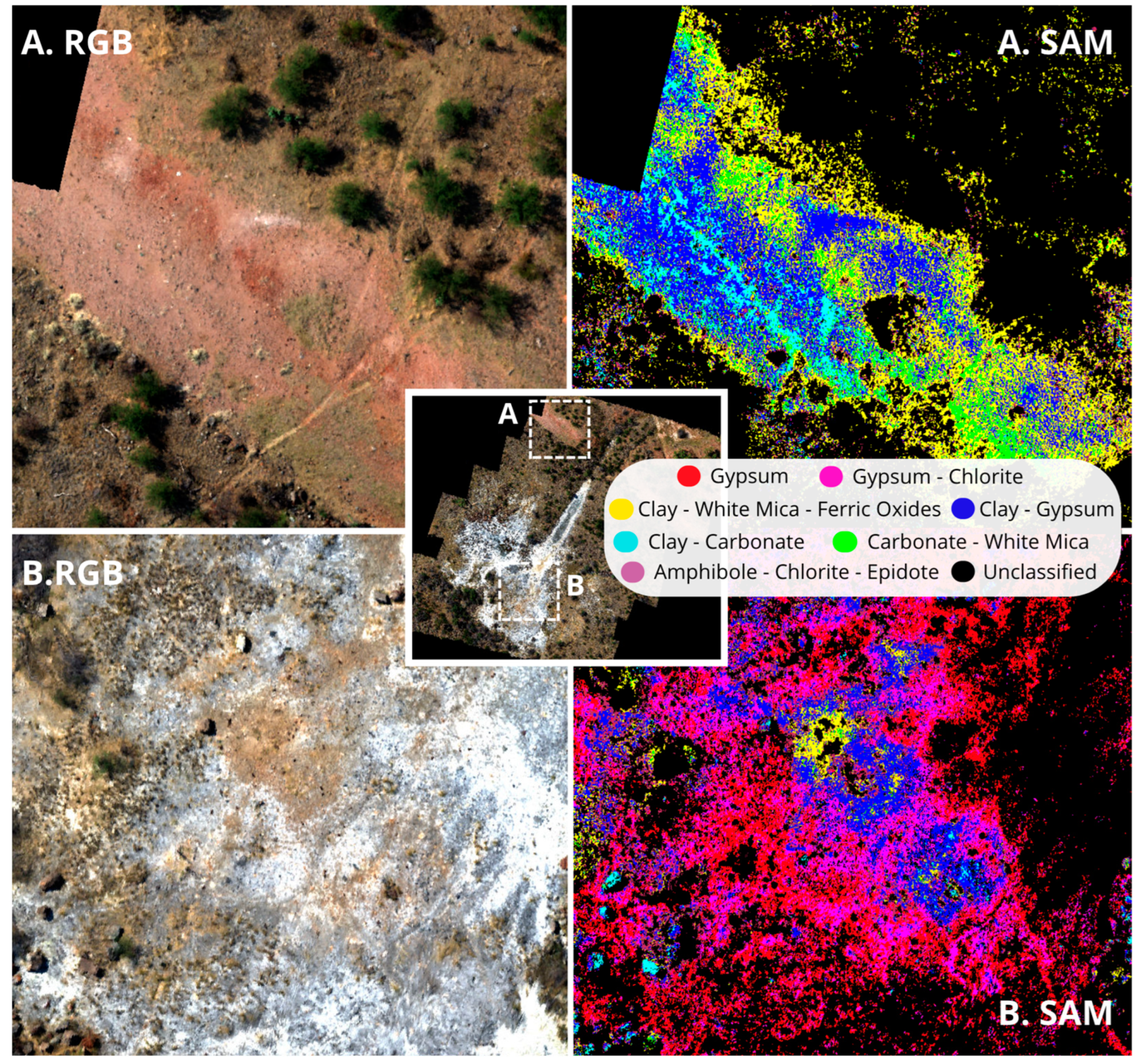
4.2. Data-Driven Mapping of Endmembers
4.3. Knowledge-Based Feature Modelling
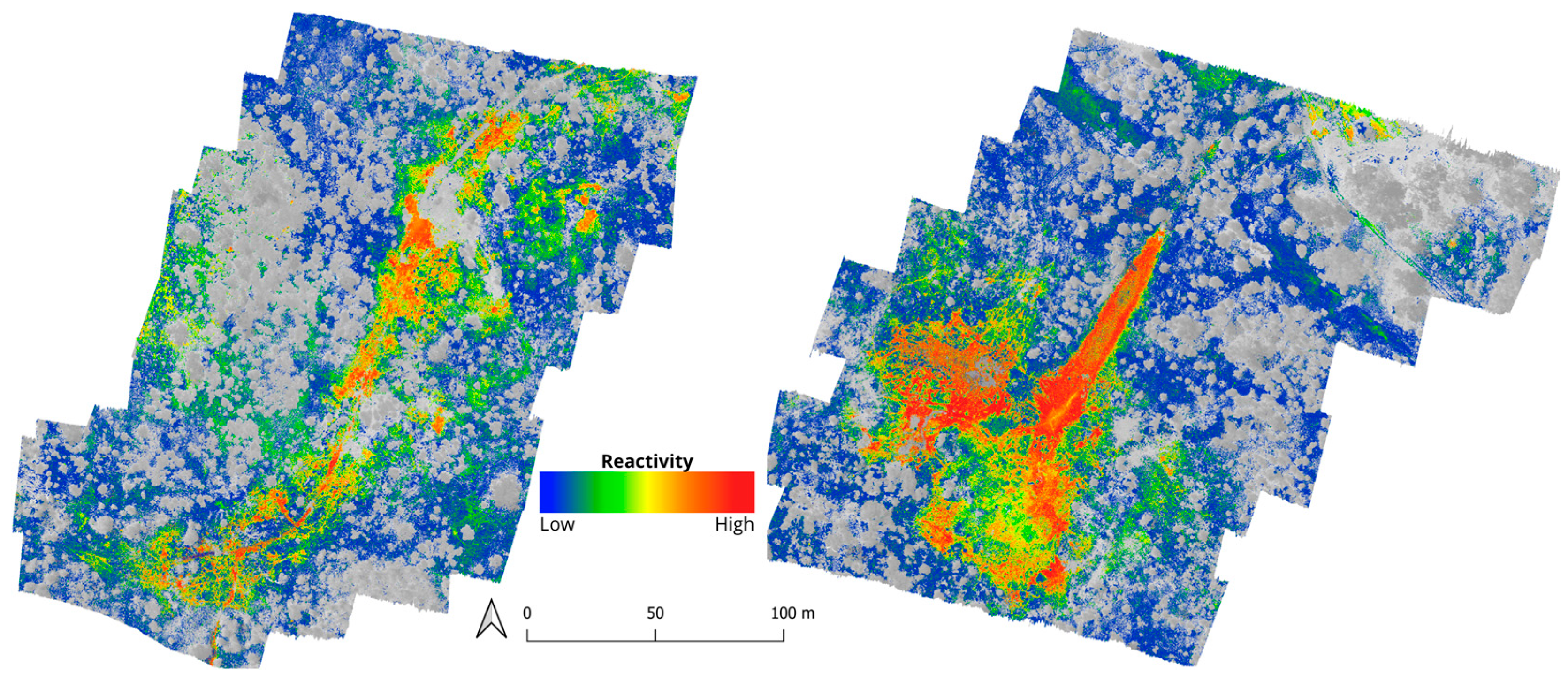
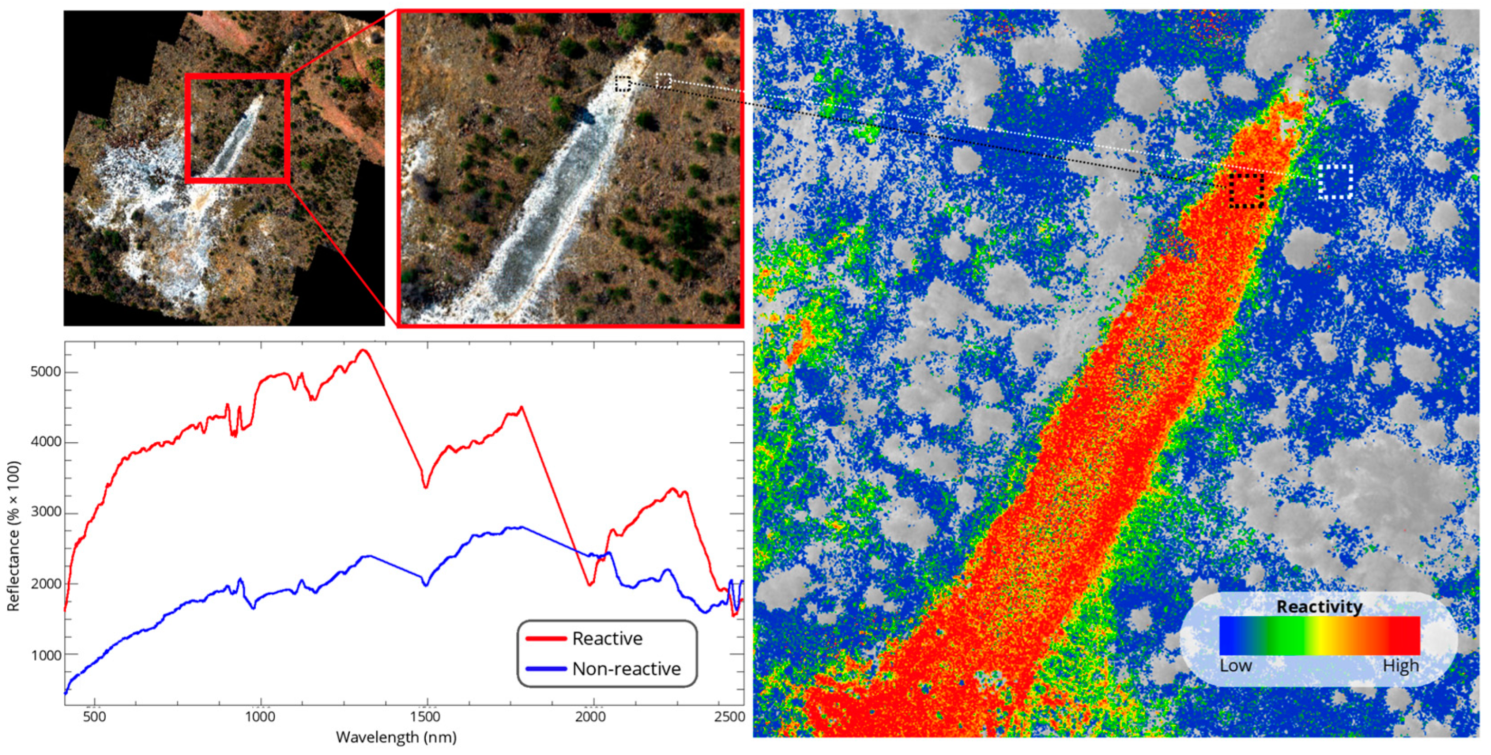
4.3.1. Mapping of Reactive Areas
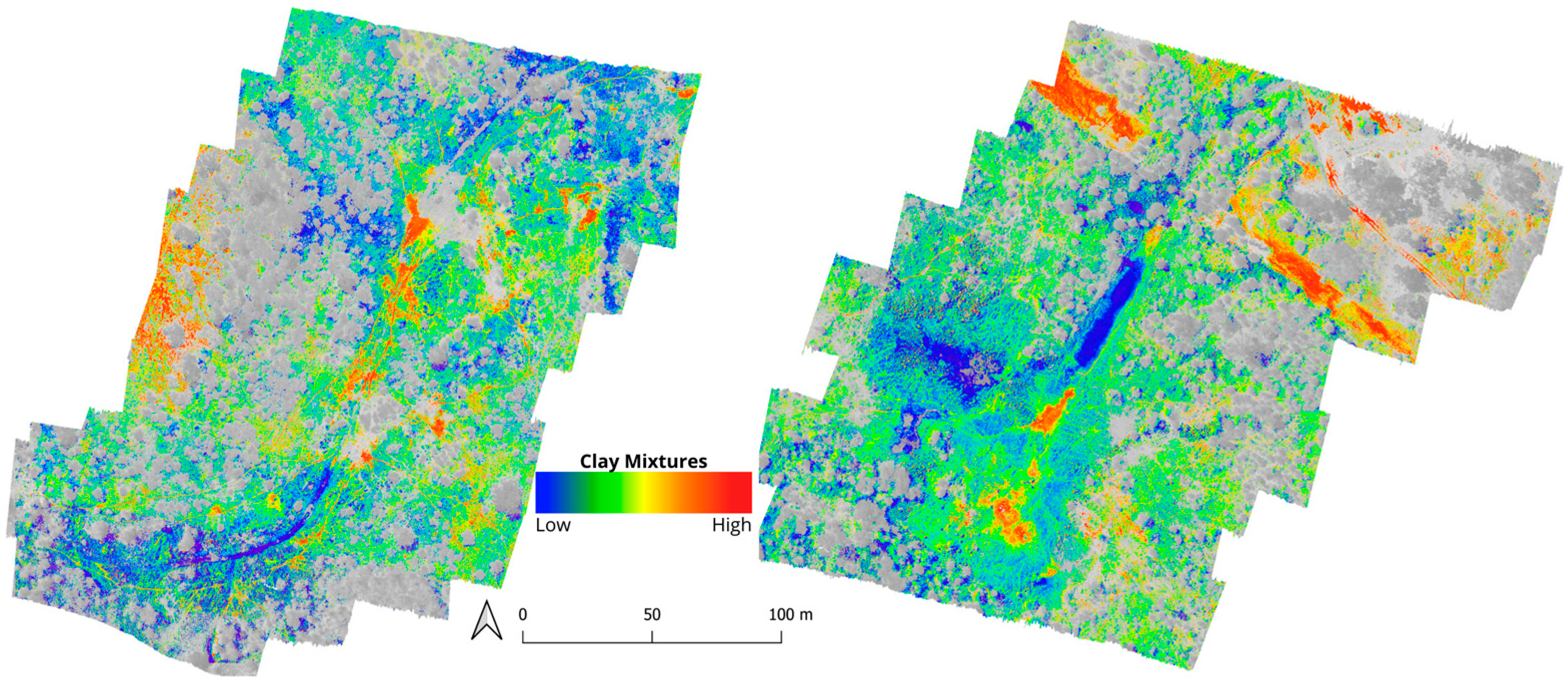
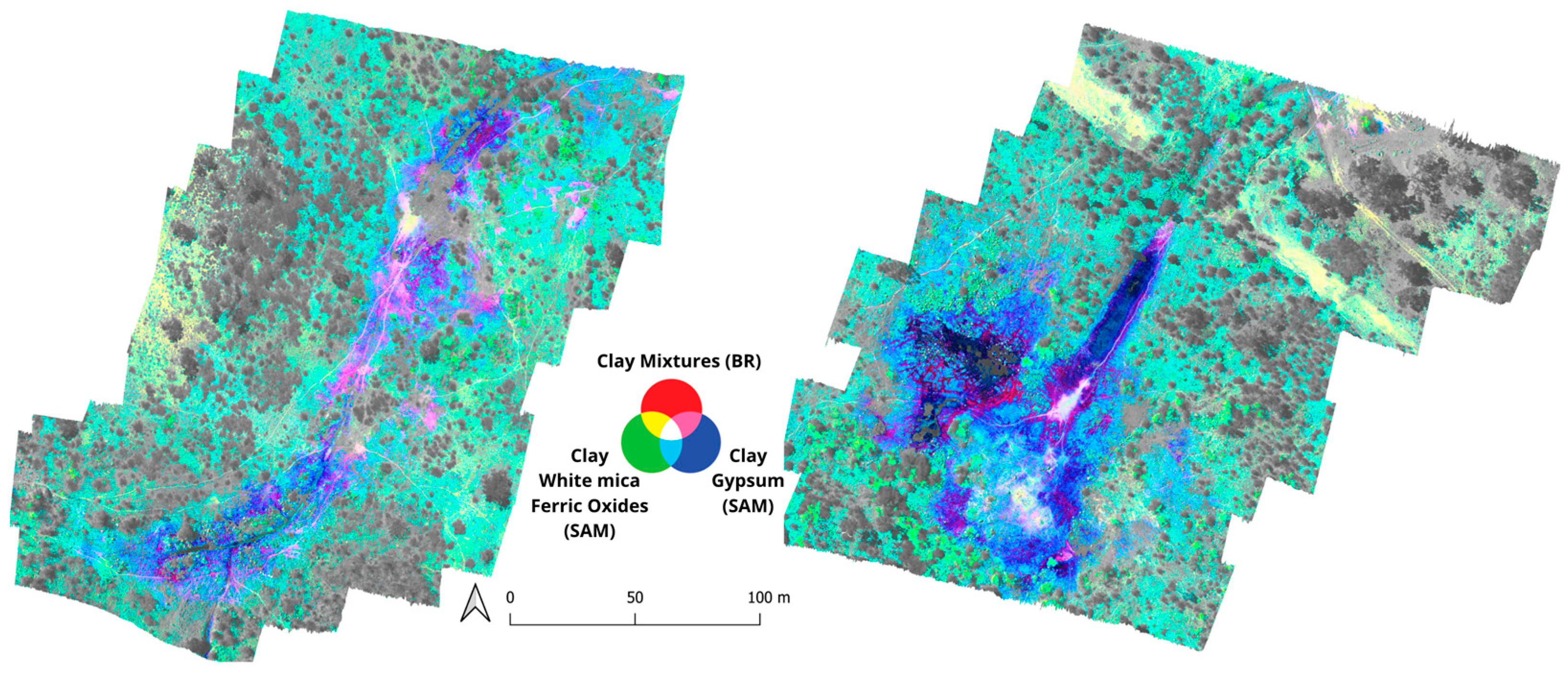
4.3.2. Mapping of Clay Mixtures
5. Discussion
5.1. Vegetation Cover
5.2. Data-Driven Mapping of Endmembers
5.3. Knowledge-Based Feature Modelling
6. Conclusions
Author Contributions
Funding
Data Availability Statement
Acknowledgments
Conflicts of Interest
Abbreviations
| Hyperspectral Imaging | HSI |
| Visible to near-infrared | VNIR |
| Shortwave infrared | SWIR |
| Spectral Angle Mapper | SAM |
| Band Ratio | BR |
| Electromagnetic radiation | EMR |
| Uncrewed Aerial System | UAS |
| Ground sampling distance | GSD |
| M4Mining | Multi-scale, Multi-sensor Mapping and Dynamic Monitoring for Sustainable Extraction and Safe Closure in Mining Environments |
| HyMap | Hyperspectral Mapper by Integrated Spectronics (Australia). |
| Tailing Storage Facility | TSF |
| Evaporation pond | EP |
| Acid Mine Drainage | AMD |
| Rare Earth Element | REE |
| Light Detection and Ranging | LiDAR |
| Analytical Spectral Device | ASD |
| Global Navigation Satellite System | GNSS |
| Inertial Measurement Unit | IMU |
| Inertial Navigation System | INS |
| Digital Surface Model | DSM |
| Ground control point | GCP |
| Above ground level | AGL |
| Mary Kathleen | MK |
| Drone and Atmospheric Correction framework | DROACOR |
| Look-up table | LUT |
| Normalised Difference Vegetation Index | NDVI |
Appendix A
Appendix B
- Water vapour interpolation: interpolating absorption features. All: Interpolates 940/1130/1400 and 1800 nm absorption bands according to the sensor-specific settings;
- Cloud shadow removal: none;
- Polishing: weak, Savitzky–Golay, seven-band filter size, third order polynomial;
- Visibility estimate failed for most flights (apart from Day 2 Site 2 Flight 1, see Table A5); for all other flights it is reset to 50 km;
- Water vapour retrieval, averaging 75 image bands.
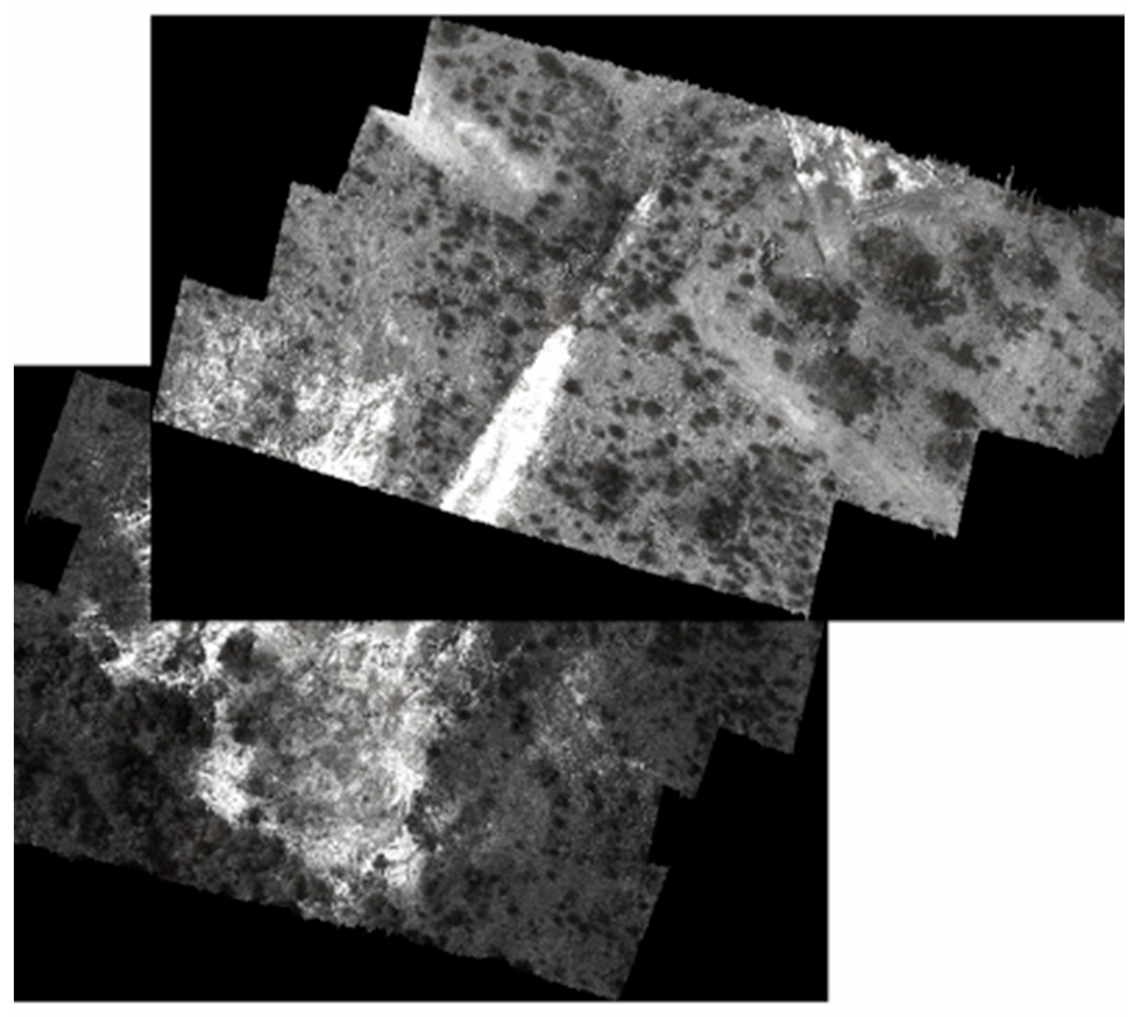
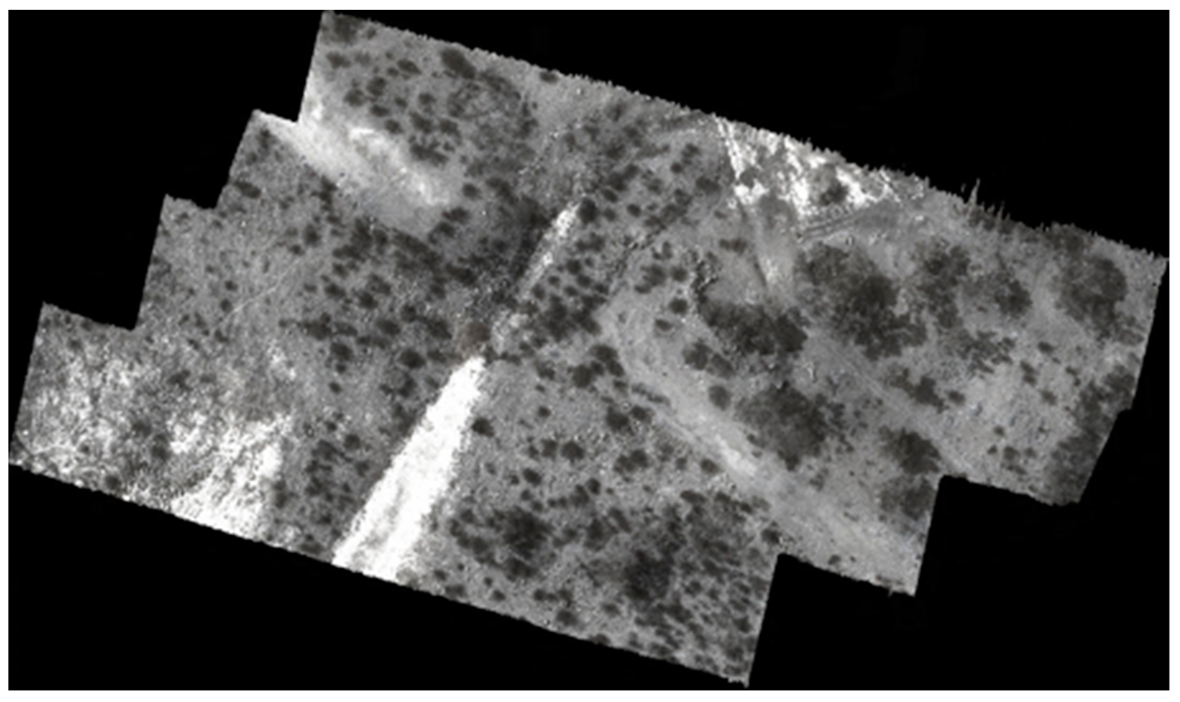
Appendix B.1. Site 1 Mosaic
Appendix B.1.1. Site 1—North (Day 2 Site 1 Flight 4)


| Flight Line ID | Scene Acquisition Date | Solar Zenith Angle [deg] | Visibility [km] | Ground Elevation [m] | Height Above Ground [m] | Average Water Vapour Column [cm] | Size of Input Image [Columns × Lines × Bands] |
|---|---|---|---|---|---|---|---|
| MK_day2_flight4_01_Mjolnir | 1 September 2023 | 32.0 | 50.0 | 371 | 119 | 1.5 | 3252 × 1179 × 487 |
| MK_day2_flight4_02_Mjolnir | 1 September 2023 | 32.1 | 50.0 | 370 | 116 | 1.5 | 3072 × 1243 × 487 |
| MK_day2_flight4_03_Mjolnir | 1 September 2023 | 32.4 | 50.0 | 369 | 119 | 1.5 | 2974 × 1116 × 487 |
Appendix B.1.2. Site 1—Centre (Day 2 Site 1 Flight 3)
| Flight Line ID | Scene Acquisition Date | Solar Zenith Angle [deg] | Visibility [km] | Ground Elevation [m] | Height Above Ground [m] | Average Water Vapour Column [cm] | Size of Input Image [Columns × Lines × Bands] |
|---|---|---|---|---|---|---|---|
| MK_day2_flight3_correct_01_Mjolnir | 1 September 2023 | 29.8 | 50.0 | 371 | 115 | 1.5 | 3430 × 1254 × 487 |
| MK_day2_flight3_correct_02_Mjolnir | 1 September 2023 | 29.9 | 50.0 | 371 | 113 | 1.5 | 2920 × 1228 × 487 |
| MK_day2_flight3_correct_03_Mjolnir | 1 September 2023 | 30.0 | 50.0 | 371 | 116 | 1.5 | 2947 × 1140 × 487 |
| MK_day2_flight3_correct_04_Mjolnir | 1 September 2023 | 30.0 | 50.0 | 371 | 112 | 1.5 | 3021 × 1280 × 487 |
Appendix B.1.3. Site 1—South (Day 4 Site 1 Flight 2)
| Flight Line ID | Scene Acquisition Date | Solar Zenith Angle [deg] | Visibility [km] | Ground Elevation [m] | Height Above Ground [m] | Average Water Vapour Column [cm] | Size of Input Image [Columns × Lines × Bands] |
|---|---|---|---|---|---|---|---|
| Day4_Site1_Flight2_03_Mjolnir | 2 September 2023 | 61.4 | 50.0 | 371 | 118 | 1.5 | 2451 × 1225 × 487 |
| Day4_Site1_Flight2_04_Mjolnir | 2 September 2023 | 61.6 | 50.0 | 371 | 112 | 1.5 | 3069 × 1252 × 487 |
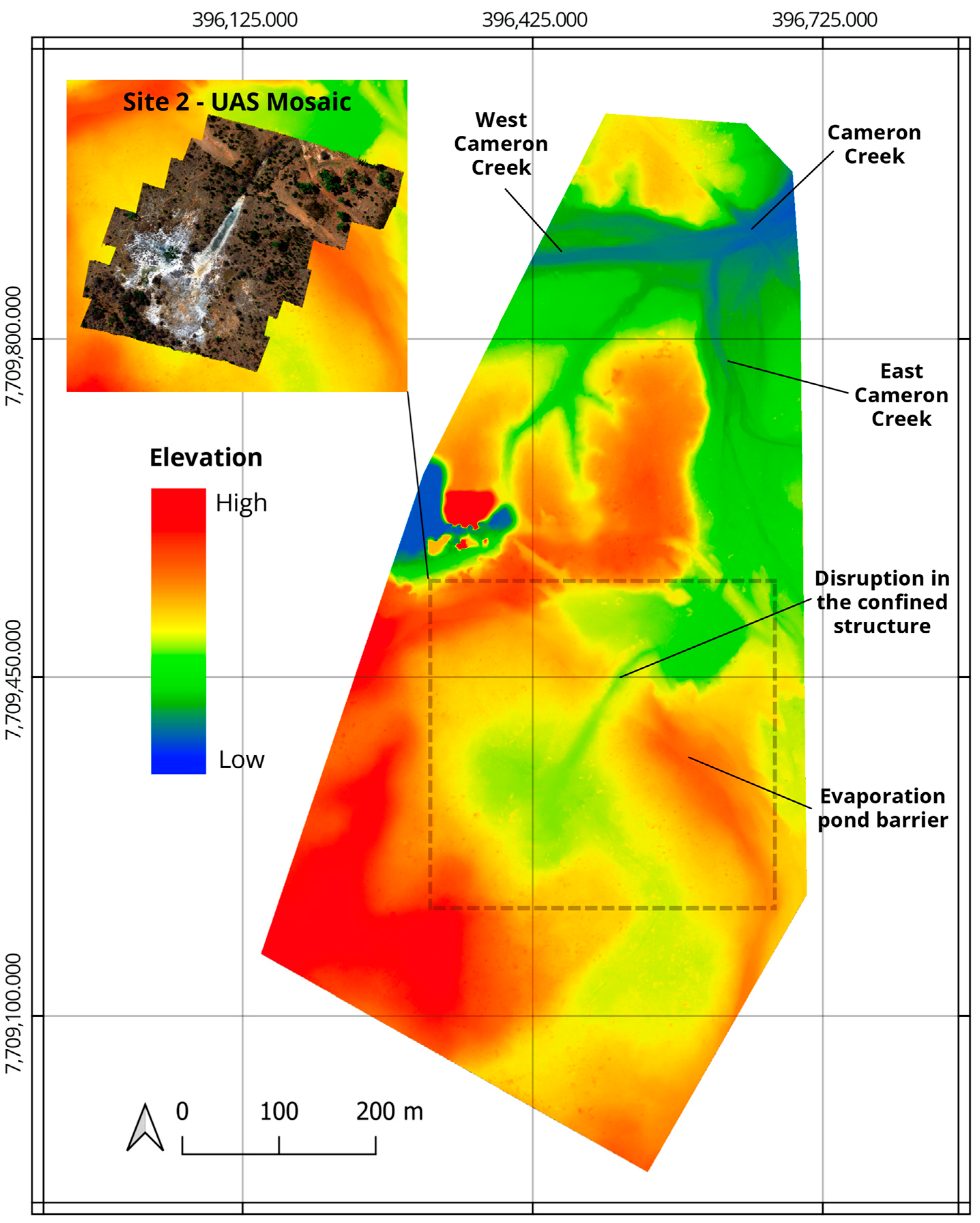
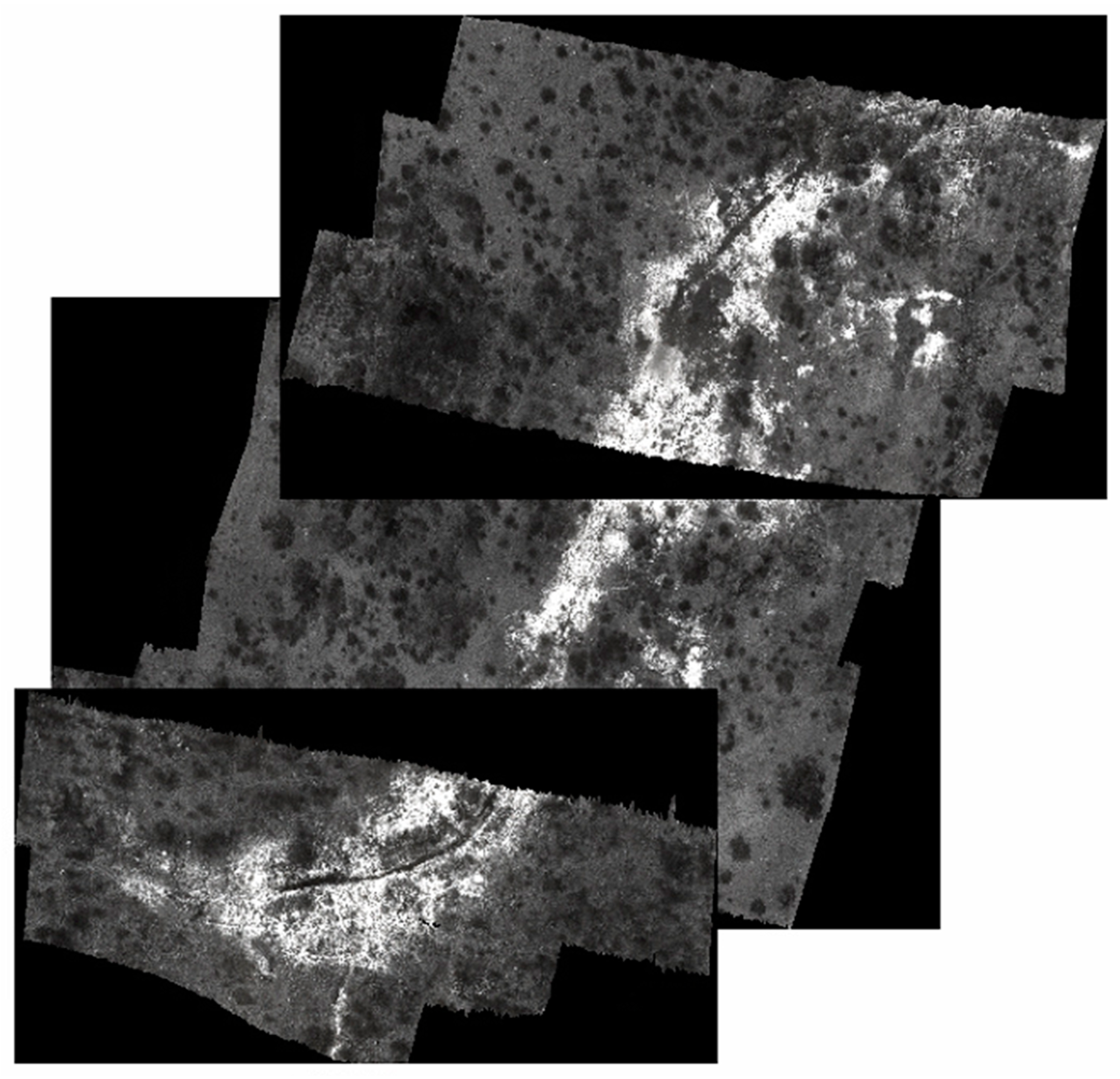
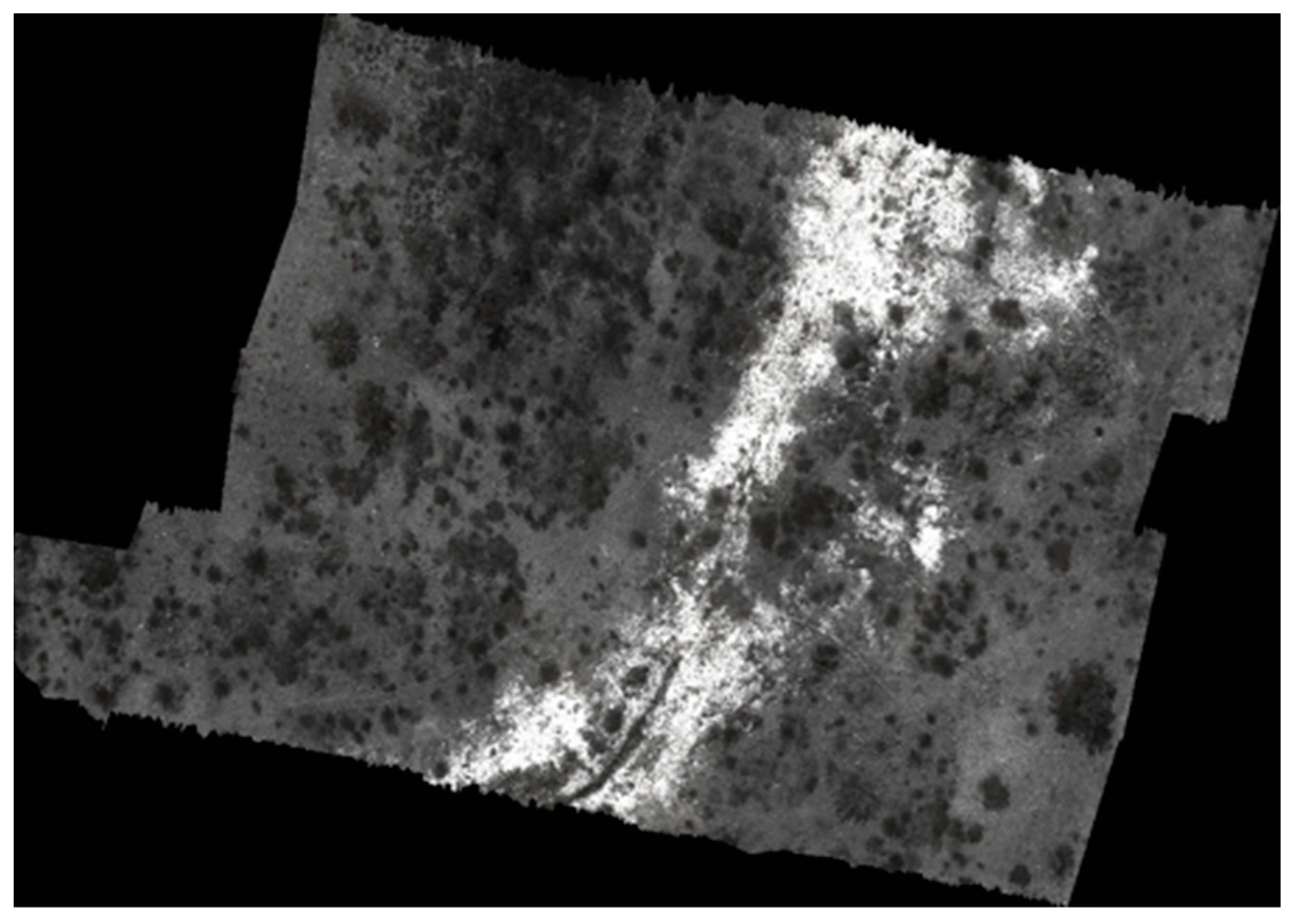
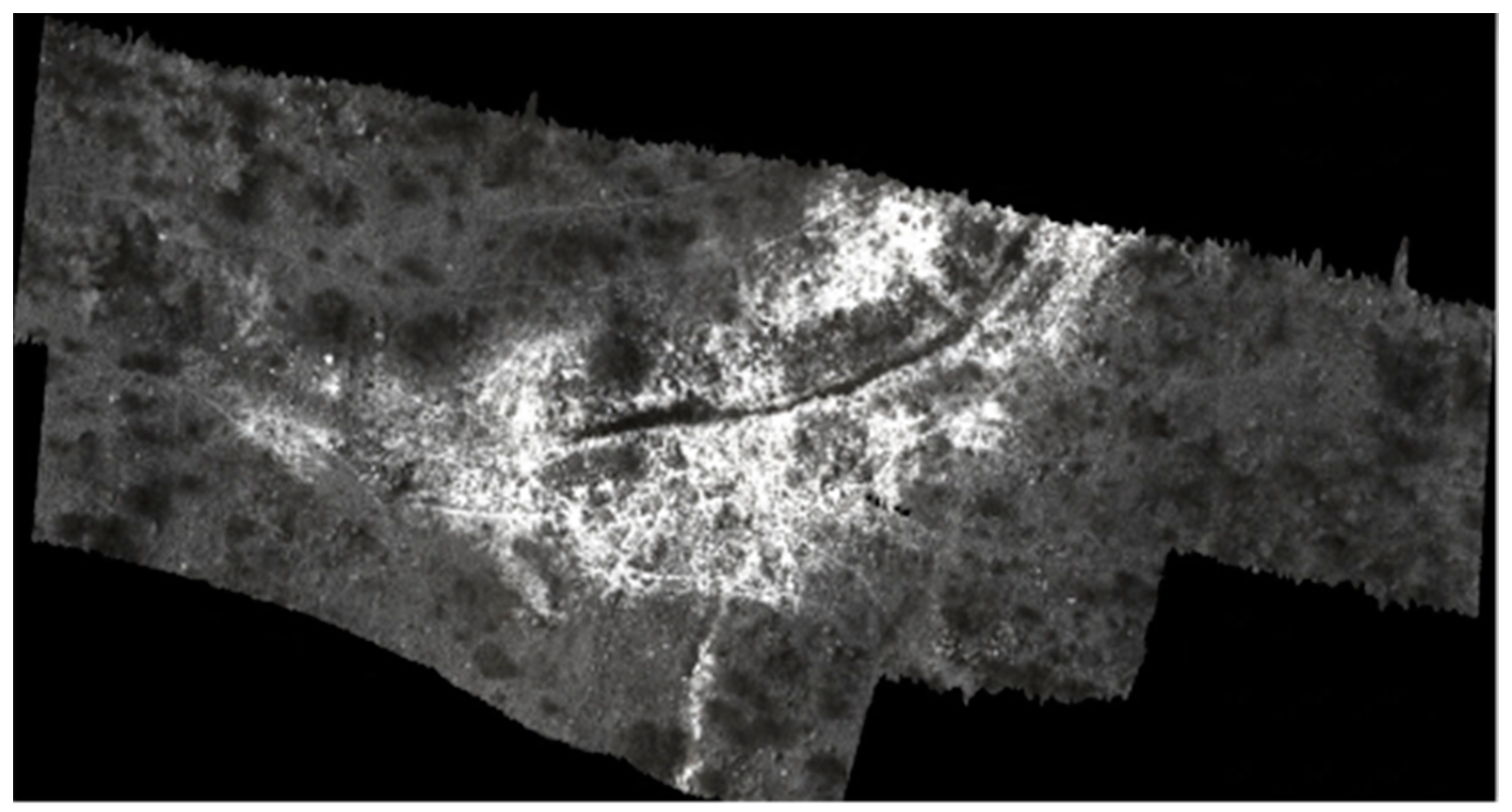
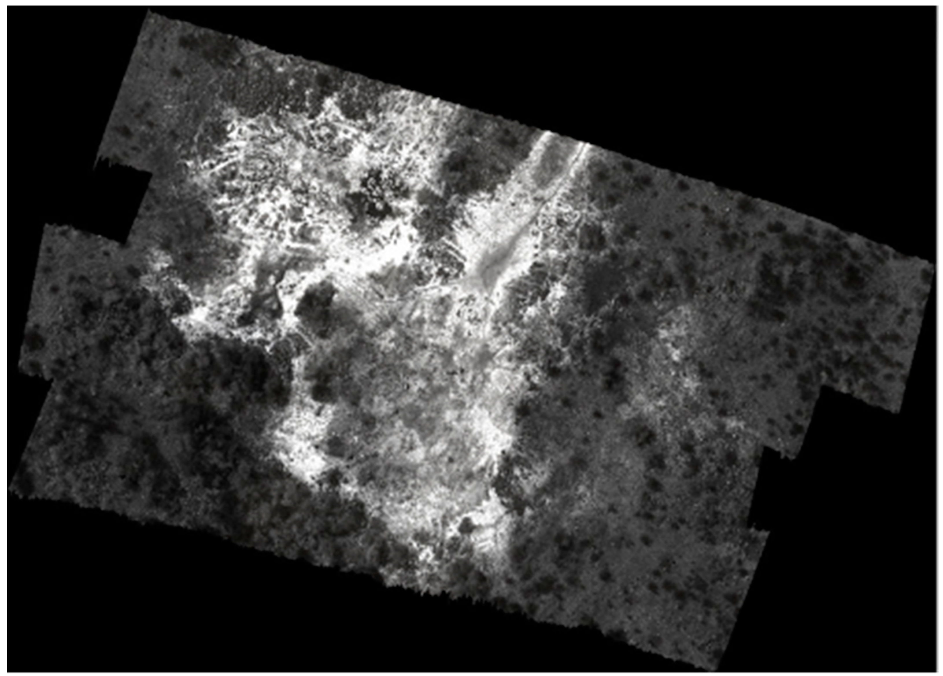
Appendix B.2. Site 2 Mosaic
Appendix B.2.1. Site 2—North (Day 2 Site 2 Flight 2)
| Flight Line ID | Scene Acquisition Date | Solar Zenith Angle [Deg] | Visibility [km] | Ground Elevation [m] | Height Above Ground [m] | Average Water Vapour Column [cm] | Size of Input Image [Columns × Lines × Bands] |
|---|---|---|---|---|---|---|---|
| MK_day2_ev2_01_Mjolnir_ | 1 September 2023 | 51.6 | 50.0 | 362 | 119 | 1.7 | 3258 × 1638 × 487 |
| MK_day2_ev2_02_Mjolnir | 1 September 2023 | 51.8 | 50.0 | 363 | 115 | 1.8 | 3437 × 1706 × 487 |
| MK_day2_ev2_03_Mjolnir | 1 September 2023 | 52.2 | 50.0 | 362 | 117 | 1.8 | 3989 × 1677 × 487 |
| MK_day2_ev2_04_Mjolnir | 1 September 2023 | 52.6 | 50.0 | 361 | 115 | 1.8 | 3704 × 1720 × 487 |
Appendix B.2.2. Site 2—South (Day 2 Site 2 Flight 1)
| Flight Line ID | Scene Acquisition Date | Solar Zenith Angle [deg] | Visibility [km] | Ground Elevation [m] | Height Above Ground [m] | Average Water Vapour Column [cm] | Size of Input Image [Columns × Lines × Bands] |
|---|---|---|---|---|---|---|---|
| MK_day2_ev1_01_Mjolnir | 1 September 2023 | 45.9 | 50.0 | 483 | 1 | 1.8 | 3804 × 1847 × 487 |
| MK_day2_ev1_02_Mjolnir | 1 September 2023 | 46.1 | 50.0 | 320 | 160 | 1.5 | 3311 × 1463 × 487 |
| MK_day2_ev1_03_Mjolnir | 1 September 2023 | 46.5 | 24 | 320 | 162 | 1.5 | 3392 × 1592 × 487 |
| MK_day2_ev1_04_Mjolnir | 1 September 2023 | 46.6 | 80 | 321 | 160 | 1.5 | 3445 × 1457 × 487 |
References
- IEA. The Role of Critical Minerals in Clean Energy Transitions. World Energy Outlook 2021. Available online: https://www.iea.org/reports/the-role-of-critical-minerals-in-clean-energy-transitions (accessed on 19 February 2025).
- Tang, L.; Werner, T.T. Global mining footprint mapped from high-resolution satellite imagery. Commun. Earth Environ. 2023, 4, 134. [Google Scholar] [CrossRef]
- European Commission. Establishment of Guidelines for the Inspection of Mining Waste Facilities, Inventory and Rehabilitation of Abandoned Facilities and Review of the BREF Document No. 070307/2010/576108/ETU/C2: Final Report. Inspection, Rehabilitation and BREF–Directorate-General for the Environment of the European Commission. 2012. Available online: https://ec.europa.eu/environment/pdf/waste/mining/Inspection-Rehabilitation_BREF_report.pdf (accessed on 19 February 2025).
- UNEP. Abandoned Mines: Problems, Issues and Policy Challenges for Decision Makers. Pan-American Workshop on Abandoned Mines 2001. Available online: https://wedocs.unep.org/20.500.11822/8116 (accessed on 19 February 2025).
- Pepper, M.; Roche, C.P.; Mudd, G.M. Mining legacies–Understanding life-of-mine across time and space. In Proceedings of the Life-of-Mine Conference, Brisbane, QLD, Australia, 16–18 July 2014; pp. 445–469. [Google Scholar]
- Nash, K. Addressing legacy sites. In Towards Zero Harm: A Compendium of Papers Prepared for the Global Tailings Review; Oberle, B., Brereton, D., Mihaylova, A., Eds.; The International Council on Mining and Metals (ICMM): London, UK, 2020; pp. 126–140. [Google Scholar]
- Gupta, R.P. Remote Sensing Geology, 3rd ed.; Springer: Berlin/Heidelberg, Germany, 2018. [Google Scholar] [CrossRef]
- Campbell, J.B.; Wynne, R.H. Introduction to Remote Sensing, 5th ed.; The Guilford Press: New York, NY, USA, 2011. [Google Scholar]
- Goetz, A.F.H.; Vane, G.; Solomon, J.E.; Rock, B.N. Imaging Spectrometry for Earth Remote Sensing. Science 1985, 228, 1147–1153. [Google Scholar] [CrossRef]
- Clark, R.N. Spectroscopy of Rocks and Minerals, and Principles of Spectroscopy. In Remote Sensing for the Earth Sciences, 3rd ed.; Rencz, A.N., Ed.; John Wiley & Sons: Toronto, ON, Canada, 1999; Volume 3, pp. 3–58. [Google Scholar]
- Hunt, G.R. Spectral Signatures of Particulate Minerals in the Visible and Near Infrared. Geophysics 1977, 42, 501–513. [Google Scholar] [CrossRef]
- van der Meer, F.D.; van der Werff, H.M.A.; van Ruitenbeek, F.J.A.; Hecker, C.A.; Bakker, W.H.; Noomen, M.F.; van der Meijde, M.; Carranza, E.J.M.; de Smeth, J.B.; Woldai, T. Multi- and Hyperspectral Geologic Remote Sensing: A Review. Int. J. Appl. Earth Obs. Geoinf. 2012, 14, 112–128. [Google Scholar] [CrossRef]
- Krupnik, D.; Khan, S. Close-Range, Ground-Based Hyperspectral Imaging for Mining Applications at Various Scales: Review and Case Studies. Earth-Sci. Rev. 2019, 198, 102952. [Google Scholar] [CrossRef]
- Peyghambari, S.; Zhang, Y. Hyperspectral Remote Sensing in Lithological Mapping, Mineral Exploration, and Environmental Geology: An Updated Review. J. Appl. Remote Sens. 2021, 15, 031501. [Google Scholar] [CrossRef]
- Koerting, F.; Asadzadeh, S.; Hildebrand, J.C.; Savinova, E.; Kouzeli, E.; Nikolakopoulos, K.; Lindblom, D.; Koellner, N.; Buckley, S.J.; Lehman, M.; et al. VNIR-SWIR Imaging Spectroscopy for Mining: Insights for Hyperspectral Drone Applications. Mining 2024, 4, 1013–1057. [Google Scholar] [CrossRef]
- Chalkley, R.; Crane, R.A.; Eyre, M.; Hicks, K.; Jackson, K.-M.; Hudson-Edwards, K.A. A Multi-Scale Feasibility Study into Acid Mine Drainage (AMD) Monitoring Using Same-Day Observations. Remote Sens. 2022, 15, 76. [Google Scholar] [CrossRef]
- Heincke, B.; Jackisch, R.; Saartenoja, A.; Salmirinne, H.; Rapp, S.; Zimmermann, R.; Pirttijärvi, M.; Vest Sörensen, E.; Gloaguen, R.; Ek, L.; et al. Developing Multi-Sensor Drones for Geological Mapping and Mineral Exploration: Setup and First Results from the MULSEDRO Project. Geol. Surv. Den. Greenl. Bull. 2019, 43, e2019430302. [Google Scholar] [CrossRef]
- Booysen, R.; Jackisch, R.; Lorenz, S.; Zimmermann, R.; Kirsch, M.; Nex, P.A.M.; Gloaguen, R. Detection of REEs with Lightweight UAV-Based Hyperspectral Imaging. Sci. Rep. 2020, 10, 17450. [Google Scholar] [CrossRef]
- Booysen, R.; Lorenz, S.; Jackisch, R.; Gloaguen, R.; Madriz, Y. How Can Drones Contribute to Mineral Exploration? In Proceedings of the 2021 IEEE International Geoscience and Remote Sensing Symposium (IGARSS); IEEE: Piscataway, NJ, USA, 2021; pp. 1867–1870. [Google Scholar] [CrossRef]
- Kirsch, M.; Lorenz, S.; Zimmermann, R.; Tusa, L.; Möckel, R.; Hödl, P.; Booysen, R.; Khodadadzadeh, M.; Gloaguen, R. Integration of Terrestrial and Drone-Borne Hyperspectral and Photogrammetric Sensing Methods for Exploration Mapping and Mining Monitoring. Remote Sens. 2018, 10, 1366. [Google Scholar] [CrossRef]
- Barton, I.F.; Gabriel, M.J.; Lyons-Baral, J.; Barton, M.D.; DuPlessis, L.; Roberts, C. Extending Geometallurgy to the Mine Scale with Hyperspectral Imaging: A Pilot Study Using Drone- and Ground-Based Scanning. Min. Metall. Explor. 2021, 38, 799–818. [Google Scholar] [CrossRef]
- He, J.; Barton, I. Hyperspectral Remote Sensing for Detecting Geotechnical Problems at Ray Mine. Eng. Geol. 2021, 292, 106261. [Google Scholar] [CrossRef]
- He, J.; DuPlessis, L.; Barton, I. Heap Leach Pad Mapping with Drone-Based Hyperspectral Remote Sensing at the Safford Copper Mine, Arizona. Hydrometallurgy 2022, 211, 105872. [Google Scholar] [CrossRef]
- Jackisch, R.; Lorenz, S.; Zimmermann, R.; Möckel, R.; Gloaguen, R. Drone-Borne Hyperspectral Monitoring of Acid Mine Drainage: An Example from the Sokolov Lignite District. Remote Sens. 2018, 10, 385. [Google Scholar] [CrossRef]
- Robinson, J.; Kinghan, P. Using Drone-Based Hyperspectral Analysis to Characterize the Geochemistry of Soil and Water. J. Geol. Resour. Eng. 2018, 6, 4. [Google Scholar] [CrossRef]
- Flores, H.; Lorenz, S.; Jackisch, R.; Tusa, L.; Contreras, I.; Zimmermann, R.; Gloaguen, R. UAS-Based Hyperspectral Environmental Monitoring of Acid Mine Drainage Affected Waters. Minerals 2021, 11, 182. [Google Scholar] [CrossRef]
- Arroyo-Mora, J.; Kalacska, M.; Inamdar, D.; Soffer, R.; Lucanus, O.; Gorman, J.; Naprstek, T.; Schaaf, E.; Ifimov, G.; Elmer, K.; et al. Implementation of a UAV–Hyperspectral Pushbroom Imager for Ecological Monitoring. Drones 2019, 3, 12. [Google Scholar] [CrossRef]
- Cudahy, T.; Jones, M.; Thomas, M.; Laukamp, C.; Caccetta, M.; Hewson, R.; Rodger, A.; Verrall, M. Next Generation Mineral Mapping: Queensland Airborne HyMap and Satellite ASTER Surveys 2006–2008. In Queensland Mineral Mapping Project Final Report (P2007/364); CSIRO: Bentley, WA, Australia, 2008. [Google Scholar]
- Salles, R. New Insights on the Mary Kathleen Metamorphic-Hydrothermal U-REE Deposit, Northwest Queensland, Australia. Ph.D. Thesis, Universidade Estadual de Campinas, São Paulo, Brazil, 2010. [Google Scholar] [CrossRef]
- Salles, R.R.; de Souza Filho, C.R.; Cudahy, T.; Vicente, L.E.; Monteiro, L.V.S. Hyperspectral Remote Sensing Applied to Uranium Exploration: A Case Study at the Mary Kathleen Metamorphic-Hydrothermal U-REE Deposit, NW, Queensland, Australia. J. Geochem. Explor. 2017, 179, 36–50. [Google Scholar] [CrossRef]
- Costelloe, M. Environmental Review of the Mary Kathleen Uranium Mine. Master’s Thesis, James Cook University, Brisbane, QLD, Australia, 2003. [Google Scholar]
- Lottermoser, B.; Ashley, P. Assessment of rehabilitated uranium mine sites, Australia. In Uranium, Mining and Hydrogeology, 1st ed.; Merkel, J.B., Hasche-Berger, A., Eds.; Springer: Berlin/Heidelberg, Germany, 2008; pp. 335–340. [Google Scholar] [CrossRef]
- Lottermoser, B.G.; Ashley, P.M.; Costelloe, M.T. Contaminant dispersion at the rehabilitated Mary Kathleen uranium mine, Australia. Environ. Geol. 2005, 48, 748–761. [Google Scholar] [CrossRef]
- Lottermoser, B.G.; Ashley, P.M. Tailings dam seepage at the rehabilitated Mary Kathleen uranium mine, Australia. J. Geochem. Explor. 2005, 85, 119–137. [Google Scholar] [CrossRef]
- Google Earth Pro 7.3.6.9796: September 20, 2022. GDA 94–MGA Zone 54, Eye Altitude 7 km. Airbus Earth Observation Satellite. Available online: https://earth.google.com/ (accessed on 19 February 2025).
- Vegafria, M.C. Geochemical Pathways of Contaminants Through Weathering of Uranium Tailings. Ph.D. Thesis, The University of Queensland, Brisbane, QLD, Australia, 2019. [Google Scholar] [CrossRef]
- Ward, T.A.; Cox, B.J. Rehabilitation of the Mary Kathleen uranium mining and processing site. In Proceedings of the 9th International Symposium Uranium and Nuclear Energy, London, UK, 5–7 September 1984; pp. 222–236. [Google Scholar]
- Ward, T.A. Rehabilitation of the Mary Kathleen Mine; MKU—Mary Kathleen Uranium Ltd.: Mary Kathleen, QLD, Australia, 1986. [Google Scholar]
- ASD Inc. ASD HaloTrek Field Guide. Malvern Panalytical Ltd. 2021. Available online: https://www.malvernpanalytical.com/en/learn/knowledge-center/user-manuals/asdhalotrekfieldguide (accessed on 19 February 2025).
- Ortega, A.O.; Tolentino, V.; Koerting, F.; Savinova, E.; Hudson-Edwards, K.; Micklethwaite, S. Geochemical and Mineralogical Ground-Truthing of Hyperspectral UAS Data Using Field Samples. Sustainable Minerals Institute, The University of Queensland, St. Lucia, QLD, Australia, 2025. manuscript in preparation; to be submitted. [Google Scholar]
- Bishop, J.L.; Lane, M.D.; Dyar, M.D.; King, S.J.; Brown, A.J.; Swayze, G.A. Spectral properties of Ca-sulfates: Gypsum, bassanite, and anhydrite. Am. Mineral. 2014, 99, 2105–2115. [Google Scholar] [CrossRef]
- Laukamp, C.; Rodger, A.; LeGras, M.; Lampinen, H.; Lau, I.C.; Pejcic, B.; Stromberg, J.; Francis, N.; Ramanaidou, E. Mineral physicochemistry underlying feature-based extraction of mineral abundance and composition from shortwave, mid, and thermal infrared reflectance spectra. Minerals 2021, 11, 347. [Google Scholar] [CrossRef]
- Schläpfer, D.; Trim, S. PARGE Version 4.0 User Manual (207.90); ReSe Applications LLC: Wil, Switzerland, 2024. [Google Scholar]
- Schläpfer, D.; Popp, C.; Richter, R. Drone data atmospheric correction concept for multi- and hyperspectral imagery—The DROACOR model. ISPRS Arch. Photogramm. Remote Sens. Spat. Inf. Sci. 2020, XLIII-B3, 473–478. [Google Scholar] [CrossRef]
- Schläpfer, D.; Richter, R.; Popp, C.; Nygren, P. DROACOR® reflectance retrieval for hyperspectral mineral exploration using a ground-based rotating platform. ISPRS Arch. Photogramm. Remote Sens. Spat. Inf. Sci. 2021, XLIII-B3, 209–214. [Google Scholar] [CrossRef]
- Schläpfer, D.; Raebsamen, J.; Popp, C.; Richter, R.; Trim, S.A.; Vögtli, M. DROACOR topographic correction method with adaptive diffuse irradiance-based shadow correction. In Proceedings of the International Geoscience and Remote Sensing Symposium–IGARSS 2023 IEEE, Pasadena, CA, USA, 16–21 July 2023; pp. 7332–7335. [Google Scholar]
- Emde, C.; Buras-Schnell, R.; Kylling, A.; Mayer, B.; Gasteiger, J.; Hamann, U.; Kylling, J.; Richter, B.; Pause, C.; Dowling, T.; et al. The libRadtran software package for radiative transfer calculations (version 2.0.1). Geosci. Model Dev. 2016, 9, 1647–1672. [Google Scholar] [CrossRef]
- Mustard, J.F.; Sunshine, J.M. Spectral Analysis for Earth Science Investigation. In Remote Sensing for the Earth Sciences, 3rd ed.; Rencz, A.N., Ed.; John Wiley & Sons: Toronto, ON, Canada, 1999; Volume 3, pp. 251–305. [Google Scholar]
- Asadzadeh, S.; de Souza Filho, C.R. A review on spectral processing methods for geological remote sensing. Int. J. Appl. Earth Obs. Geoinf. 2016, 47, 69–90. [Google Scholar] [CrossRef]
- Landgrebe, D.A. Signal Theory Methods in Multispectral Remote Sensing, 1st ed.; John Wiley & Sons: New York, NY, USA, 2003. [Google Scholar] [CrossRef]
- Booysen, R.; Lorenz, S.; Thiele, S.T.; Fuchsloch, W.C.; Marais, T.; Nex, P.A.M.; Gloaguen, R. Accurate hyperspectral imaging of mineralised outcrops: An example from lithium-bearing pegmatites at Uis, Namibia. Remote Sens. Environ. 2022, 269, 112790. [Google Scholar] [CrossRef]
- Agar, B.; Coulter, D.W. Remote Sensing for Mineral Exploration: A Decade Perspective 1997–2007. In Proceedings of the Fifth Decennial International Conference on Mineral Exploration, Toronto, ON, Canada, 22–25 October 2007; pp. 109–136. [Google Scholar]
- Henrich, V.; Krauss, G.; Götze, C.; Sandow, C. Index DataBase (IDB)-Development of a Database for Remote Sensing Indices; AK Fernerkundung: Bochum, Germany, 2012; Available online: www.indexdatabase.de (accessed on 19 February 2025).
- Yuhas, R.H.; Goetz, A.F.; Boardman, J.W. Discrimination among semi-arid landscape endmembers using the spectral angle mapper (SAM) algorithm. In Summaries of the Third Annual JPL Airborne Geoscience Workshop; Realmuto, V.J., Ed.; Jet Propulsion Lab: Pasadena, CA, USA, 1992; Volume 2, pp. 147–149. [Google Scholar]
- Kruse, F.A.; Lefkoff, A.B.; Boardman, J.W.; Heidebrecht, K.B.; Shapiro, A.T.; Barloon, P.J.; Goetz, A.F.H. The spectral image processing system (SIPS)–Interactive visualization and analysis of imaging spectrometer data. Remote Sens. Environ. 1993, 44, 145–163. [Google Scholar] [CrossRef]
- Gupta, D.V.; Areendran, G.; Raj, K.; Ghosh, S.; Dutta, S.; Sahana, M. Assessing habitat suitability of leopards (Panthera pardus) in unprotected scrublands of Bera, Rajasthan, India. In Forest Resources Resilience and Conflicts; Shit, P.K., Pourghasemi, H.R., Adhikary, P.P., Bhunia, G.S., Sati, V.P., Eds.; Elsevier: Amsterdam, The Netherlands, 2021; pp. 329–342. [Google Scholar] [CrossRef]
- Navarro-Ramos, S.E.; Sparacino, J.; Rodríguez, J.M.; Filippini, E.; Marsal-Castillo, B.E.; García-Cannata, L.; Renison, D.; Torres, R.C. Active revegetation after mining: What is the contribution of peer-reviewed studies? Heliyon 2022, 8, e09179. [Google Scholar] [CrossRef]


| Data Source/Instrument | Spectral Range | Nº. Bands | Spectral Sampling | Spatial Resolution |
|---|---|---|---|---|
| In situ measurements: ASD TerraSpec Halo 1 | 350–2500 nm | 358 | 6 nm | Single measurements, spot size of 1 × 1 cm |
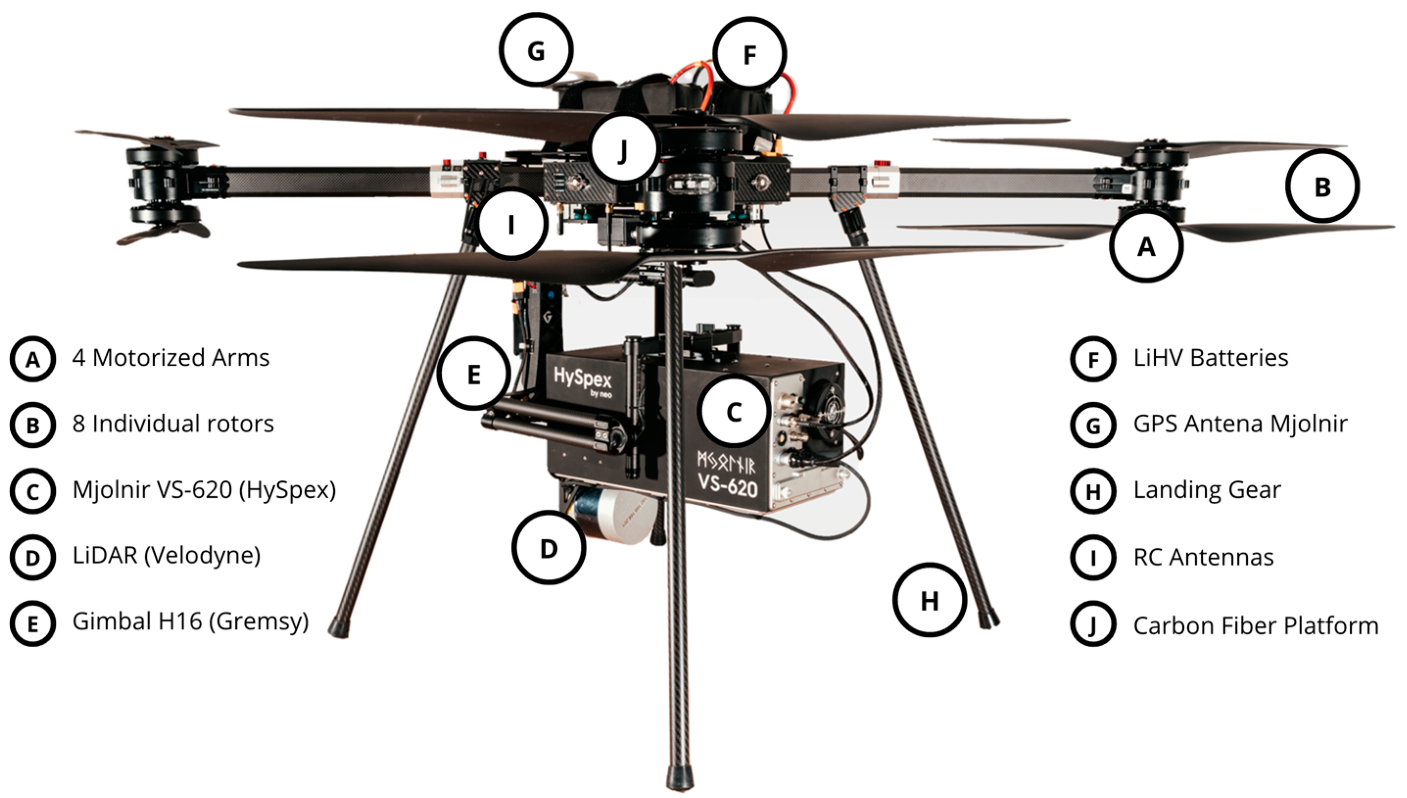
| UAS: HySpex Mjolnir VS-620 2 | 400–2500 nm | 410 | 3 nm (VNIR); 5.1 nm (SWIR) | 6–10 cm |
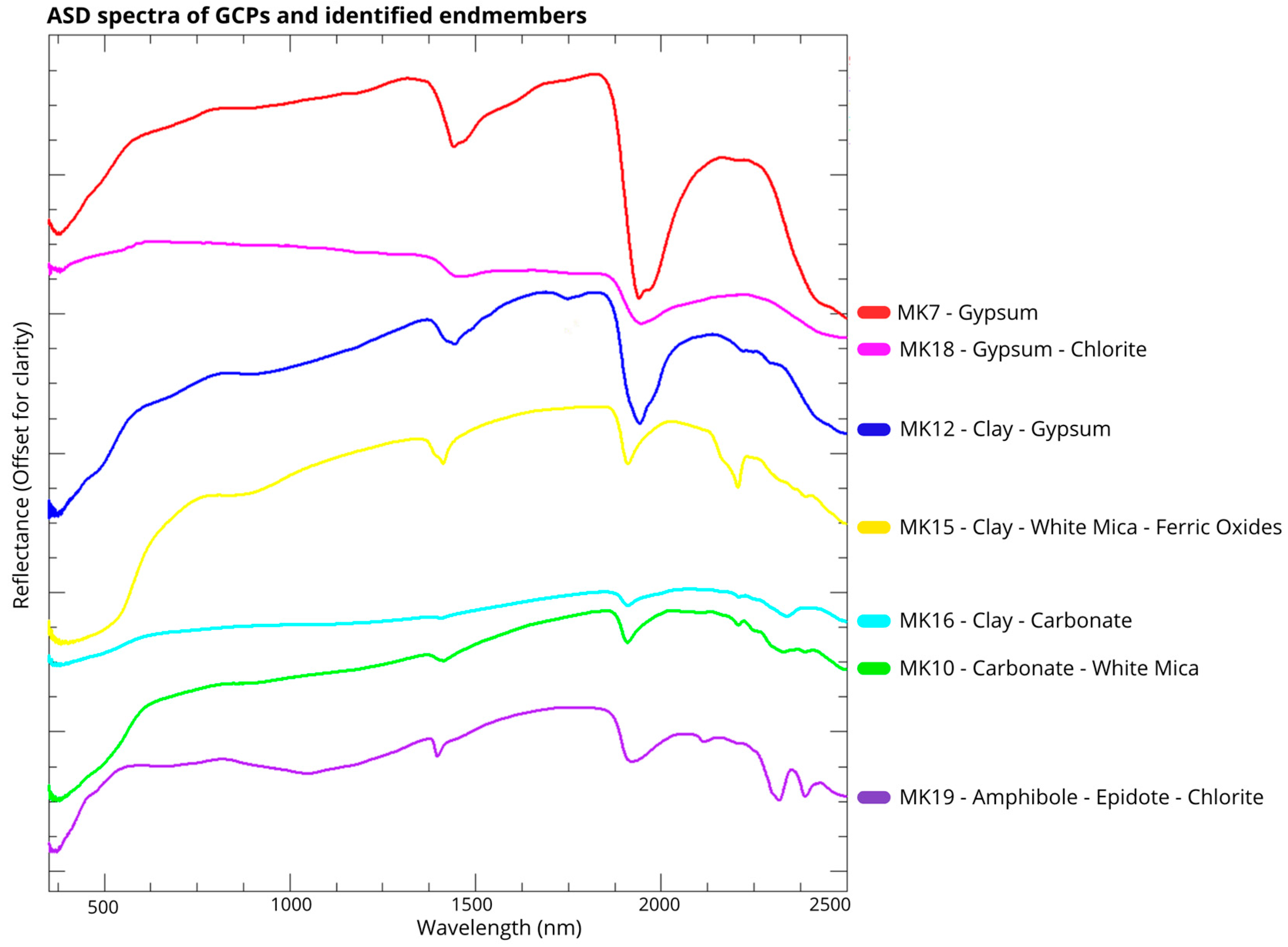
| Endmember | GCP ID 1 | Spectral Features 2 | Surface Pattern 3 |
|---|---|---|---|
| Gypsum | MK7 | 1400 nm; 1580 nm; 1750 nm | Evaporitic sediments |
| Gypsum–Chlorite | MK18 | 1750 nm; 2260 nm | Evaporitic sediments |
| Clay–Gypsum | MK12 | 1750 nm; 2200 nm | Early phase of evaporites formation |
| Clay–White Mica–Ferric Oxide | MK15 | 520 nm; 860 nm; 2200 nm; 2350 nm | Clay and soil surficial layers |
| Clay–Carbonate | MK16 | 2200 nm; 2340 nm | Waste rock capping (rehabilitation) |
| Carbonate–White Mica | MK10 | 2155 nm; 2250 nm; 2340 nm | Waste rock capping (rehabilitation) |
| Amphibole–Epidote–Chlorite | MK19 | 2260 nm; 2320 nm; 2390 nm | Stable surfaces |
| Band Ratio 1 | Formula | Index Range | Targeted Surface Pattern |
|---|---|---|---|
| NDVI | (800 nm − 678 nm) ÷ (800 nm + 678 nm) | −1.00–1.00 | Vegetation covers |
| Reactivity | (2210 nm + 2395 nm) ÷ (2285 nm + 2330 nm) | 0.66–2.11 | Reactive areas |
| Clay Mixtures | (2168 nm × 2224 nm) ÷ (2198 nm) | 1.15–4.34 | Clay mixtures |
Disclaimer/Publisher’s Note: The statements, opinions and data contained in all publications are solely those of the individual author(s) and contributor(s) and not of MDPI and/or the editor(s). MDPI and/or the editor(s) disclaim responsibility for any injury to people or property resulting from any ideas, methods, instructions or products referred to in the content. |
© 2025 by the authors. Licensee MDPI, Basel, Switzerland. This article is an open access article distributed under the terms and conditions of the Creative Commons Attribution (CC BY) license (https://creativecommons.org/licenses/by/4.0/).
Share and Cite
Tolentino, V.; Ortega Lucero, A.; Koerting, F.; Savinova, E.; Hildebrand, J.C.; Micklethwaite, S. Drone-Based VNIR–SWIR Hyperspectral Imaging for Environmental Monitoring of a Uranium Legacy Mine Site. Drones 2025, 9, 313. https://doi.org/10.3390/drones9040313
Tolentino V, Ortega Lucero A, Koerting F, Savinova E, Hildebrand JC, Micklethwaite S. Drone-Based VNIR–SWIR Hyperspectral Imaging for Environmental Monitoring of a Uranium Legacy Mine Site. Drones. 2025; 9(4):313. https://doi.org/10.3390/drones9040313
Chicago/Turabian StyleTolentino, Victor, Andres Ortega Lucero, Friederike Koerting, Ekaterina Savinova, Justus Constantin Hildebrand, and Steven Micklethwaite. 2025. "Drone-Based VNIR–SWIR Hyperspectral Imaging for Environmental Monitoring of a Uranium Legacy Mine Site" Drones 9, no. 4: 313. https://doi.org/10.3390/drones9040313
APA StyleTolentino, V., Ortega Lucero, A., Koerting, F., Savinova, E., Hildebrand, J. C., & Micklethwaite, S. (2025). Drone-Based VNIR–SWIR Hyperspectral Imaging for Environmental Monitoring of a Uranium Legacy Mine Site. Drones, 9(4), 313. https://doi.org/10.3390/drones9040313