Multi-Mode Flight Simulation and Energy-Aware Coverage Path Planning for a Lift+Cruise QuadPlane

Abstract

This paper describes flight planning supported by modeling, guidance, and feedback control for an electric Vertical Take-Off and Landing (eVTOL) QuadPlane small Uncrewed Aircraft System (sUAS). Five Lift+Cruise sUAS waypoint types are defined and used to construct smooth flight path geometries and acceleration profiles. Novel accelerated coverage flight plan segments for hover (Lift) and coverage (Cruise) waypoint types are defined as a complement to traditional fly-over, fly-by, and Dubins path waypoint transit solutions. Carrot-chasing guidance shows a tradeoff between tracking accuracy and control stability as a function of the carrot time step. Experimentally validated aerodynamic and thrust models for vertical, forward, and hybrid flight modes are developed as a function of airspeed and angle of attack from wind tunnel data. A QuadPlane feedback controller augments classical multicopter and fixed-wing controllers with a hybrid control mode that combines multicopter and aircraft control actuators to add a controllable pitch degree of freedom at the cost of increased energy use. Multi-mode flight simulations show Cruise mode to be the most energy efficient with a relatively large turning radius constraint, while quadrotor mode enables hover and smaller radius turns. Energy efficiency analysis over QuadPlane plans with modest inter-waypoint distances indicates cruise or aircraft mode is $30\%$ more energy efficient overall than quadrotor mode. Energy-aware coverage planner simulation results show fly-coverage (cruise) waypoints are always the most efficient given long distances between waypoints. A Pareto analysis of energy use versus area coverage is presented to analyze waypoint-type tradeoffs in case studies with closely spaced waypoints. Coverage planning and guidance methods from this paper can be applied to any Lift+Cruise aircraft configuration requiring waypoint flight mode optimization over energy and coverage metrics.

1. Introduction

Urban Air Mobility [1,2], expanded to Advanced Air Mobility [3,4], is expected to be a disruptive technology that leverages electric Vertical Take-off and Landing (eVTOL) platforms. Several eVTOL concepts have been proposed [5] and broadly categorized [6] as Multicopter [7,8], Side-by-Side Helicopter [9], Lift+Cruise [10], and Tiltwing [11]. Lift+Cruise configurations are desirable because they offer energy-efficient cruise as well as hover and vertical take-off and landing capability. Small Uncrewed Aircraft Systems (sUAS) eVTOL aircraft engaged in package delivery, surveillance, and mapping missions also benefit from a Lift+Cruise configuration. This paper investigates multi-mode planning and guidance for a QuadPlane [12], a Lift+Cruise sUAS modeled with aerodynamic data collected from wind tunnel experiments [13,14].

The QuadPlane is a superposition of a quadcopter over a conventional fixed-wing sUAS layout designed for mid-range sUAS missions requiring eVTOL capability. Figure 1 shows the QuadPlane schematic and prototype introduced in [12] and used for wind tunnel testing in [13,14]. Like all Lift+Cruise aircraft, it operates in three primary flight modes distinguished by their flight envelopes and control actuation: Quad (Lift), Plane (Cruise), and Hybrid. Quad mode uses only the four vertical thrust pusher motors for control actuation. Plane mode uses only the forward tractor motor, ailerons, elevator, and rudder, and Hybrid mode uses all propulsion units and control surfaces.

This paper first defines five waypoint types to generate multi-mode eVTOL flight plans with smooth turns and acceleration. Trajectory generation utilizes novel hover (Lift) and coverage (Cruise) waypoint types tailored to Lift+Cruise sUAS while also supporting conventional fly-over, fly-by, and Dubins path waypoint traversals. Flight planning methods ensure compatibility of adjacent waypoint types subject to trajectory and aircraft performance constraints. An Energy-Aware Coverage path planner is introduced, providing the option to prioritize energy efficiency or path coverage in the selection of waypoint sequence types. Inter-waypoint flight segments incorporate optimal traversal between hover waypoints from [15] and otherwise exhibit cruise flight with optimal transitions to and from hover as needed. Carrot guidance with adjustable carrot time step horizons supports multi-mode trajectory tracking while providing a tradeoff between tracking accuracy and controller stability. A novel combination of conventional aircraft and multicopter control laws enables sustained operations in Hybrid mode and unlocks an additional pitch-tracking degree of freedom while tracking a desired translational trajectory. Multi-mode QuadPlane aerodynamic and propulsion models are developed from wind tunnel test data [14]. Analysis of trim states, power consumption, and transitions between flight modes provides insights for energy-efficient flight planning methods. Guidance and control simulations are shown in zero and steady ambient wind conditions. Case studies for Energy-Aware Coverage path planning with sensitivity analysis and Pareto front analysis are presented.

Specific contributions of this work include the following:

1

Energy Aware Coverage path planning that utilizes novel hover and coverage waypoint types to construct Lift+Cruise flight plans that optimally trade-off path coverage with energy efficiency. Transitions between lift and cruise modes are incorporated as required.

2

A guidance protocol that enables the QuadPlane to “crab” up to ${180}^{\circ }$ into the wind to maximize stability with zero sideslip when prescribed the airspeed is less than ambient steady wind speed.

3

A QuadPlane flight controller offering stable multi-mode flight, including transitions. Simulation results highlight the additional Hybrid mode pitch tracking degree of freedom.

4

An experimentally derived eVTOL sUAS aerodynamic model for all QuadPlane flight modes expressed as a function of airspeed and angle of attack.

5

Energy-efficient trim states in all three flight modes. Range and endurance in each flight mode are also modeled to define sUAS mission constraints.

6

A Pareto analysis of energy versus coverage metrics as a function of waypoint sequence proximity and types.

Below, Section 2 provides a literature review followed by aircraft nonlinear dynamics preliminaries in Section 3. Section 4 describes five waypoint types and corresponding trajectory generation solutions. Section 5 describes energy-efficient multi-mode eVTOL sUAS flight planning methods, including the Energy Aware Coverage path planner. eVTOL guidance and control solutions are described in Section 6. Section 7 presents experimentally derived aerodynamic and propulsion models and trim state analysis for the QuadPlane. Section 8 presents simulation results in individual flight modes with and without ambient wind, as well as waypoint flight sequences with energy-aware coverage planning. A Pareto analysis offers insight into the energy use versus coverage trade space. A discussion in Section 9 is followed by conclusions in Section 10.

2. Literature Review

This section summarizes relevant literature in aircraft dynamics, guidance, control, flight planning, and minimum energy trajectory optimization.

2.1. Vertical Take-Off and Landing Aircraft Dynamics

Aerodynamic modeling for Lift+Cruise aircraft such as the QuadPlane requires modeling both vertical (quadrotor) and forward (fixed-wing) flight dynamics. Fixed-wing aircraft dynamics models are well established, as shown in [16,17,18]. Although the full nonlinear model is typically used for flight simulation, when aggressive maneuvering is not required, the feedback controller can be linearized around a set of trim states with gain scheduling [19,20]. Multicopters are modeled from the thrust and moments generated by individual propulsion modules as described in [21]. Multirotor models include drag from the spinning propellers as a linear function of the multicopter velocity in addition to body drag.

Early Vertical Take-off and Landing aircraft such as the V-22 Osprey faced initial challenges during transitions between vertical and forward flight [22,23]. Recently, distributed electric propulsion [24] has enabled electric Vertical Take Off and Landing (eVTOL) aircraft designs. For small unmanned aircraft systems (sUAS), the Aerosonde model released in 2001 [25] is commonly used for academic research. The Zagi flying-wing model is also available in [18] with aerodynamic coefficients required to carry out realistic dynamics simulations. Authors in [26] present two loosely engineered eVTOL concepts—one, which has co-axial rotors on each quadcopter arm, and the other with two tilt-wings. Accurate aerodynamic modeling for eVTOL aircraft is important to understand the impact of flow interactions when designing robust transition controllers. Although numerous eVTOL aircraft designs have been proposed in the industry [5], models are considered confidential and are not available for public use. eVTOL sUAS flight dynamics modeling with Computational Fluid Dynamics (CFD) is described in [27]. The authors of [28] conducted wind tunnel tests to model the performance of a Tilt-Rotor eVTOL aircraft, while [29] shows a performance analysis of a tandem wing long-range eVTOL concept. The QuadPlane from [13,14] is an alternative fixed-wing Lift+Cruise design for which experimental datasets have been collected to model performance. This paper describes QuadPlane dynamics in the style of [16,18,21] with experimental data from [13,14] in guidance, control, and simulation studies.

2.2. Guidance and Control

Several strategies have been proposed for trajectory tracking or path following for ground and air vehicles. Geometric techniques initially proposed for missile guidance are now commonly used for airplane and multicopter guidance, including carrot-chasing, line-of-sight, and pure pursuit guidance algorithms. The carrot-chasing algorithm [30] is a simple geometric strategy that steers the aircraft toward a Virtual Target Point (VTP) located on the path. The VTP is at a constant distance ahead of the prescribed flight path. Line-of-sight [31] steers the aircraft toward the closest point on the desired trajectory, while the Pure Pursuit algorithm [32] guides the aircraft straight to a target point on the desired path. Ref. [33] surveys available guidance strategies. A modified version of the Carrot-Chasing algorithm [30] is used for QuadPlane guidance in this paper, offering a trade-off between robust control and tracking accuracy by varying the time horizon or carrot time steps.

The QuadPlane is a hybrid system with three distinct continuous dynamical modes (quadrotor, fixed-wing plane, and the hybrid combination of both) linked by discrete transition events. A hybrid system control [34] approach is utilized in controller design. In this paper, the control system merges strategies from the fixed-wing aircraft and multicopter literature to create a seamless control model for the QuadPlane’s overall flight conditions. The authors in [16,35,36] describe methods for classical and modern control system design for fixed-wing aircraft with conventional aileron, elevator, and rudder control surfaces. Ref. [18] describes successive proportional–integral–derivative (PID) loop closure control for fixed-wing aircraft. Ref. [21] describes successive PID control loops to track lateral position, altitude, and yaw with a multicopter design. The authors in [26] present a review of four Advanced Air Mobility vehicle types from a control perspective. A full-flight envelope nonlinear control scheme is presented in [37] for a conceptual Lift+Cruise Advanced Air Mobility aircraft. For the QuadPlane, the Plane (fixed wing) mode control design follows Ref. [18]. Quad (vertical) mode control design follows Ref. [21] and the open-source flight software rc_pilot (https://github.com/StrawsonDesign/rc_pilot, accessed on 11 June 2024). Hybrid mode uses a novel combination of the Plane and Quad mode flight controllers as described below in Section 6.2.

2.3. Flight Planning and Energy-Efficient Traversal

Time-synchronized waypoints describing the position coordinates ($x,y,z$) and arrival time t define flight missions [38]. In [39], the authors describe a pseudo-spectral approach to connect waypoints with a smooth trajectory. The FAA describes two methods of constructing a reference trajectory with waypoints: “Fly-By” ($FB$) and “Fly-Over” ($FO$) [40]. “Fly-By” waypoints require an aircraft to begin turning to the next course angle prior to reaching the waypoint connecting two route segments. “Fly-Over” waypoints require the aircraft to fly directly over each waypoint and then initiate a turn to point along a radial to the next waypoint. In Section 4.1, we utilize Fly-By and Fly-Over waypoints and introduce “Fly-Coverage” and “Hover” waypoints suitable for eVTOL sUAS inspection and surveillance missions.

Energy-efficient trajectory generation in a steady wind field for a fixed-wing [41,42] and multicopter [43] Uncrewed Aircraft Systems (UAS) have been studied for single-flight mode operations. This paper extends prior work by considering flight mode switching to improve energy efficiency and coverage path tracking. In-flight trajectory optimization in [44] has shown improvements in fuel savings at the potential cost of operator and controller task load. Applications such as phenotyping require coverage path planning, as seen in [45], where the authors developed a tool to enhance small UAS autopilot with optical remote sensing workflows. The authors in [46] provide a systematic review of coverage route planning techniques for UAS. Recent work has investigated optimal control application to eVTOL flight planning. For example, Ref. [47] applies optimal control to the National Aeronautics and Space Administration (NASA) Lift+Cruise aircraft concept [6], though pure cruise mode is not utilized since vertical motors generate thrust at nontrivial power use even at cruise airspeeds. Energy-efficient direct accelerated trajectories between hover waypoint pairs are presented in our previous work [15]. This paper uses the optimal traversals from [15] to approach and depart from hover waypoints and extends this analysis to support coverage path planning over all other waypoint types defined below.

3. Preliminaries

Nonlinear, six degrees of freedom body axes equations [16,17,21] model QuadPlane dynamics in all flight modes:

$$\begin{array}{cc}\hfill \overrightarrow{\dot{X}}& \hfill =f(\overrightarrow{X},{\overrightarrow{u}}_P,{\overrightarrow{u}}_Q).\hfill \end{array}$$

(1)

In state vector $\overrightarrow{X}={\left[\begin{array}{c}xyzuvw\varphi \theta \psi pqr\end{array}\right]}^T$, ($x,y,z$) denotes position in the inertial (Earth) frame; ($u,v,w$) denotes velocity in the body frame; ($\varphi ,\theta ,\psi$) are the Euler angles for roll, pitch and yaw; and ($p,q,r$) are body frame angular rates. The Plane mode control vector ${\overrightarrow{u}}_P={\left[\begin{array}{cccc}{\delta }_a& {\delta }_e& {\delta }_r& T_{fwd}\end{array}\right]}^T$ contains normalized aileron, elevator and rudder deflections, and forward thrust, respectively. The Quad mode control vector ${\overrightarrow{u}}_Q={\left[\begin{array}{cccc}{T}_1& T_2& T_3& T_4\end{array}\right]}^T$ contains the four vertical motor thrust values. In Hybrid mode, both ${\overrightarrow{u}}_Q$ and ${\overrightarrow{u}}_P$ are active.

The nonlinear function $f(.)$ in Equation (1) defines force and moment dynamics as well as inertial position and Euler angle kinematics. Body (B) to Earth (E) frame rotation matrix (${}^E\mathbf{R}_B$) is defined to compute inertial velocity ($\dot{x},\dot{y},\dot{z}$) from body frame translational velocity ($u,v,w$). Euler angle kinematics define ($\dot{\varphi },\dot{\theta },\dot{\psi }$) from the body frame angular velocity vector ($p,q,r$) per [16]. Translational and angular body frame accelerations are governed by the force and moment equations per

$$\begin{array}{cc}\dot{u}\hfill & =rv-qw-gsin\theta +F_x/m,\hfill \\ \dot{v}\hfill & =-ru+pw+gsin\varphi cos\theta +F_y/m,\hfill \\ \dot{w}\hfill & =qu-pv+gcos\varphi cos\theta +F_z/m,\hfill \\ \dot{p}\hfill & ={\displaystyle \frac{1}{\mathsf{{\rm Y}}}}[J_{xz}[J_x-J_y+J_z]pq-[J_z(J_z-J_y)+J_{xz}^2]qr+J_z{M}_x+J_{xz}{M}_z],\hfill \\ \dot{q}\hfill & ={\displaystyle \frac{1}{J_y}}[(J_z-J_x)pr-J_{xz}(p^2-r^2)+M_y,\hfill \\ \dot{r}\hfill & ={\displaystyle \frac{1}{\mathsf{{\rm Y}}}}[[(J_x-J_y)J_x+J_{xz}^2]pq-J_{xz}[J_x-J_y+J_z]qr+J_{xz}{M}_x+J_x{M}_z],\hfill \end{array}$$

(2)

where $\mathsf{{\rm Y}}=J_x{J}_z-J_{xz}^2$, ($J_x,J_y,J_z$) = $(0.12,0.07,0.11)$ kg m² are the QuadPlane principal moments of inertia, and $J_{xy}=J_{yz}=0$ due to QuadPlane symmetry. $J_{xz}=1.6\times {10}^{-4}$ kg m². QuadPlane moments of inertia were experimentally determined using the bifilar pendulum experiment described in [21]. Total force $\overrightarrow{F}{|}_B={\left[\begin{array}{ccc}{F}_x& F_y& F_z\end{array}\right]}^T$ and moment $\overrightarrow{M}{|}_B={\left[\begin{array}{ccc}{M}_x& M_y& M_z\end{array}\right]}^T$ acting on the QuadPlane in the body frame arise from a combination of aerodynamics and propulsion, i.e., $\overrightarrow{F}={\overrightarrow{F}}_A+{\overrightarrow{F}}_T$ and $\overrightarrow{M}={\overrightarrow{M}}_A+{\overrightarrow{M}}_T$. Section 7 describes aerodynamic (${\overrightarrow{F}}_A,{\overrightarrow{M}}_A$) and propulsion (${\overrightarrow{F}}_T,{\overrightarrow{M}}_T$) forces and moments acting on the aircraft in each flight mode at a given airspeed and angle of attack. We assume small angles for roll and pitch to prevent gimbal lock. A $z-y-x$ Euler angle convention is used, while coordinate frames and aerodynamic angle conventions are adopted from [16].

Wind vector ${\overrightarrow{V}}^w{|}_I=\left[\begin{array}{ccc}{V}_x^w& V_y^w& 0\end{array}\right]$ is defined to analyze aircraft motion in steady horizontal wind with magnitude $V^w=\sqrt{{V_x^w}^2+{V_y^w}^2}$ and heading ${\sigma }^w=ta{n}^{-1}(V_y^w/V_x^w)$. By convention, wind blowing from the South towards North has ${\sigma }^w=0$. For constant altitude flight in steady wind, airspeed $V^a$, heading $\sigma$, ground speed $V^g$, and course angle $\chi$ are related as follows:

$$\begin{array}{ccc}\dot{x}=V^{g}cos\left(\chi \right)=V^{a}cos\left(\sigma \right)+V^{w}cos\left({\sigma }^w\right),\hfill & & \dot{y}=V^{g}sin\left(\chi \right)=V^{a}sin\left(\sigma \right)+V^{w}sin\left({\sigma }^w\right).\hfill \end{array}$$

(3)

4. Flight Planning with Lift+Cruise Waypoint Types

This section describes flight planning methods for eVTOL sUAS based on five waypoint types that dictate local Lift+Cruise mode, airspeed profile, and trajectory geometry near that waypoint. This work assumes constant flight altitude and clear airspace to focus on multi-mode guidance and control as well as energy-aware waypoint-type selection. Simulations assume the eVTOL sUAS will take off and climb vertically to the target altitude and descend vertically at the chosen landing site. Heading, course angle, and airspeed changes are governed by cubic splines to ensure smooth trajectories that minimize transient oscillations.

4.1. Waypoint Types

The five waypoint types defined in this work are Hover ($HV$), Fly-Over ($FV$), Fly-By ($FB$), Fly-Over-Dubins ($FOD$), and Fly-Coverage ($FC$). A sample trajectory for each is shown in Figure 2, where the first waypoint (green) is either Hover ($HV$), Fly-Over Dubins ($FOD$), or Fly-Coverage ($FC$), and the last waypoint (red) is Fly-Over ($FO$), while the ground track between waypoints is shown as a dashed black line. Note in Figure 2d that the velocity vector points along the next segment, indicated by the dashed black line. “Hover” ($HV$) waypoints have zero ground velocity, allowing an sUAS sensor to “stare” at a target. Commercial aviation defines “Fly-Over” ($FO$) and “Fly-By” ($FB$) waypoints [40]. The same definitions are used here. Two or more consecutive “Fly-Over-Dubins” $FOD$ waypoints define Dubins path segment(s) [48] that match position and heading at each $FOD$ waypoint. Fly-Coverage ($FC$) waypoints, introduced in this paper, are inspired by area coverage pattern flights where the reference ground track is closely followed while flying at a constant speed. $FC$ waypoints enable the aircraft to pass directly over the waypoint with the heading and course angle required for the next segment and follow the direct ground track more closely than a Dubins path, as will be shown in case studies. These objectives are accomplished with a sequence of two adjacent cubic spline turns to match the next segment heading and course angle. $HV$ waypoints require flight in Quad (Lift) mode, while all other waypoints assume flight in Plane (Cruise) mode.

The ground track between $HV$ waypoint pairs is followed by the straight-line energy-minimizing accelerated trajectory defined in [15]. All turns are executed at constant airspeed, with turns for $FO$, $FB$ and $FC$ waypoints following cubic spline(s) defined to respect maximum turn rate ${\dot{\sigma }}_{max}$. $FOD$ maintains a constant turn rate ${\dot{\sigma }}_{max}$ with a larger predefined turn radius. Ground tracks for $FO$ and $FOD$ waypoint trajectories are simple to define and pass through each waypoint, but $FO$ and $FOD$ paths deviate significantly from the direct reference ground track relative to $FC$ waypoint path segments. $FB$ waypoint trajectories provide better ground track coverage given an efficient inscribed turn but do not fly directly over each waypoint.

4.2. Flight Plan Specification:

eVTOL flight planning requires specification of a physical waypoint sequence ${\mathbf{W}}_{in}$, wind vector ${\overrightarrow{V}}^w$ and aircraft performance characteristics $\overrightarrow{A}$ as input. ${\mathbf{W}}_{in}$ is the user specified input waypoint sequence for an n-segment trajectory, containing the input waypoint types associated with each $x,y$ coordinate:

$${\mathbf{W}}_{in}=\left[\begin{array}{ccc}\overrightarrow{x}& \overrightarrow{y}& \overrightarrow{WPT}\end{array}\right]=\left[\begin{array}{ccc}{x}_1& y_1& HV\\ x_2& y_2& WP{T}_2\\ ⋮& ⋮& ⋮\\ x_n& y_n& WP{T}_n\\ x_{n+1}& y_{n+1}& HV\end{array}\right].$$

(4)

The first and last waypoints of any eVTOL trajectory are always Hover ($HV$), consistent with vertical launch and landing profiles. Intermediate waypoints can be of any type, i.e., $WP{T}_i\in \{HV,FO,FB,FOD,FC\},\forall i\in \{2,n\}$ as described in the previous subsection. As we consider constant altitude flight plans, the z-coordinate is not specified explicitly. ${\overrightarrow{V}}^w$ is the steady wind vector, and $\overrightarrow{A}=\{V_c^a,a_{max},{\dot{\sigma }}_{max},V_{QH}^a,V_{HP}^a\}$ defines pertinent aircraft dynamics, kinematics, and transition parameters. We consider cubic spline acceleration profiles for trajectory generation, which require cruise airspeed $V_c^a$, maximum acceleration magnitude $a_{max}^a$, and maximum heading rate ${\dot{\sigma }}_{max}$ over the cubic spline turns [15]. Airspeed is chosen for trajectory generation as it dictates energy consumption, flight modes, and feasibility with respect to the flight envelope. Aircraft active flight mode (M) over the trajectory is dictated by airspeed $V^a$ relative to parameters $(V_{QH}^a,V_{HP}^a)$, the Quad (Lift) to Hybrid and Hybrid to Plane (Cruise) mode transition airspeeds, respectively.

$$M=\left\{\begin{array}{cc}Quad,\hfill & \mathrm{if}{V}^a<V_{QH}^a\hfill \\ Hybrid,\hfill & \mathrm{if}{V}_{QH}^a\le V^a<V_{QH}^a\hfill \\ Plane,\hfill & \mathrm{if}{V}^a\ge V_{HP}^a.\hfill \end{array}\right.$$

(5)

The output flight plan is defined as $\mathcal{P}=\{{\mathbf{T}}_d,{\overrightarrow{WPT}}_d\}$, where ${\mathbf{T}}_d=\left[\begin{array}{c}{\overrightarrow{x}}_d{\overrightarrow{y}}_d{\overrightarrow{\dot{x}}}_d{\overrightarrow{\dot{y}}}_d{\overrightarrow{t}}_d\end{array}\right]$ is the planned trajectory matrix, which defines the desired time-synchronized position vector (${\overrightarrow{x}}_d$, ${\overrightarrow{y}}_d$), ground velocity vector (${\overrightarrow{\dot{x}}}_d$, ${\overrightarrow{\dot{y}}}_d$), and time vector (${\overrightarrow{t}}_d$) spaced evenly by time step $dt$. ${\overrightarrow{WPT}}_d$ is the desired waypoint type vector for each segment and is determined by the flight planner. The flight planner ensures waypoint types and planned paths are consistent with inter-waypoint distance and aircraft performance constraints.

4.3. Trajectory Generation

This subsection describes how trajectories are defined in known steady wind, assuming initial and final $HV$ waypoints and constant altitude for the waypoint types described above. Flight plan $\mathcal{P}$ trajectory ${\mathbf{T}}_d$ is prescribed from the sequence of trajectory segments $\{S_1,S_2,\dots ,S_n\}$. Each segment $S_i$ is a function of $WP{T}_i$, $WP{T}_{i+1}$ and $S_{i-1}$. Given five waypoint types, 25 waypoint combinations are possible for segment $S_i$ from $WP{T}_i$ to $WP{T}_{i+1}$.

Table 1. Waypoint combination constraints.

${\mathit{WPT}}_{\mathit{i}}$	${\mathit{WPT}}_{\mathit{i}+1}$	Constraints
$HV$	$HV$	$l_{i,i+1}\ge 0$
	{$FO,FB,FOD,FC$}	$l_{i,i+1}\ge d_{min}$
$FO$	{$HV,FO,FB,FOD,FC$ }	$l_{i,i+1}\ge d_{min}$
$FB$	{$HV,FO,FB,FOD,FC$ }	$l_{i,i+1}\ge d_{min}$
$FOD$	{$HV,FB,FC$ }	$WP{T}_{i-1}=FOD\wedge l_{i,i+1}\ge d_{min}$
	{$FO,FOD$}	$l_{i,i+1}\ge 0$
$FC$	{$HV,FO,FB,FOD,FC$ }	$l_{i,i+1}\ge d_{min}$

specifies waypoint pair $(WP{T}_i,WP{T}_{i+1})$ constraints. Let $l_{i,i+1}$ be the straight line distance between adjacent waypoints i and $i+1$, and let $d_{min}\ge 0$ represent the minimum segment length necessary to accommodate mode transition and/or minimum turning radius requirements for $S_i$. Input waypoint type vector $\overrightarrow{WPT}$ can either be ignored, e.g., for Energy-Aware Coverage flight planning, or can be user specified. Flight planners described in Section 5 that generate ${\overrightarrow{WPT}}_d$ from $\overrightarrow{WPT}$ modify user input waypoints as needed to meet Table 1 constraints.

Each trajectory segment $S_i$ is specified by heading $\overrightarrow{\sigma }\left(t\right)$ and airspeed ${\overrightarrow{V}}^a\left(t\right)$ time histories based on initial and final segment waypoint coordinates and types. Time t is assumed to start at zero for each segment $S_i$. $\overrightarrow{\sigma }\left(t\right)$ and ${\overrightarrow{V}}^a\left(t\right)$ can be used to compute ground velocity (${\overrightarrow{\dot{x}}}_d,{\overrightarrow{\dot{y}}}_d$) and position (${\overrightarrow{x}}_d,{\overrightarrow{y}}_d$) at each time step j:

$$\begin{array}{cccc}\hfill \overrightarrow{{\dot{x}}_d}\left(j\right)& ={\overrightarrow{V}}^a\left(i\right)cos\left(\overrightarrow{\sigma }\left(j\right)\right)+V^{w}cos\left({\sigma }^w\right),\hfill & \hfill {\overrightarrow{\dot{y}}}_d\left(j\right)& ={\overrightarrow{V}}^a\left(i\right)sin\left(\overrightarrow{\sigma }\left(j\right)\right)+V^{w}sin\left({\sigma }^w\right),\hfill \\ \hfill {\overrightarrow{x}}_d\left(j\right)& ={\overrightarrow{x}}_d(j-1)+{\overrightarrow{\dot{x}}}_d\left(j\right)dt,\hfill & \hfill {\overrightarrow{y}}_d\left(j\right)& ={\overrightarrow{y}}_d(j-1)+{\overrightarrow{\dot{y}}}_d\left(j\right)dt.\hfill \end{array}$$

(6)

4.3.1. “Hover” Waypoint Trajectory

Three cases exist when a trajectory segment between $WP{T}_i$ and $WP{T}_{i+1}$ uses Hover waypoints: (i) $WP{T}_i=WP{T}_{i+1}=HV$; (ii) $WP{T}_i=HV$; and (iii) $WP{T}_{i+1}=HV$. For case (i), energy-optimal trajectories that accelerate, cruise when possible, and decelerate have been prescribed in [15] and are used here. In steady wind, a combination of sideslip and heading rate limits ${\dot{\sigma }}_{max}$ can make direct flight between hover waypoints impossible [15]. This paper only considers steady wind cases where straight-line traversal is possible for simplicity. With no wind, a heading change to a new course angle occurs while hovering at each $HV$ waypoint, and the aircraft weather vanes continuously as it traverses directly to the next waypoint in steady wind.

When $WP{T}_i=HV$ but $WP{T}_{i+1}\ne HV$, the aircraft accelerates from hover to cruise airspeed $V_c^a$ then continues at cruise speed $V_c^a$. Acceleration time $t_{acc}$ and straight-line distance traveled $l_{acc}$ subject to maximum acceleration constraint ($a_{max}^a$) are computed from [15]. When $WP{T}_{i+1}=HV$ but $WP{T}_i\ne HV$, the aircraft initially cruises toward $WP{T}_{i+1}$ at cruise airspeed $V_c^a$ and begins a deceleration profile to hover just in time to reach hover upon arrival at $WP{T}_{i+1}$. Deceleration time $t_{dec}$ and straight-line distance traveled $l_{dec}$ subject to a maximum deceleration limit are also computed from [15]. A direct straight-line course angle is assumed over both the accelerated and decelerated trajectory segments. The time history for heading $\sigma \left(t\right)$ given airspeed time history $V^a\left(t\right)$ and steady wind ${\overrightarrow{V}}^w$ can be computed from Equation (3).

4.3.2. “Fly-Over” Waypoint Trajectory

“Fly-Over” ($FO$) waypoints require the aircraft to pass exactly over waypoint coordinates with no restrictions on ground track and course angle as described in [40]. Our $FO$ implementation uses a cubic spline for turns for smooth roll reference trajectories that avoid a step change in roll rate. Flight at constant airspeed $V^a$ is assumed, i.e., ${\overrightarrow{V}}^a\left(t\right)=V^a,\forall t$. Let ($x_1,y_1$) and ($x_3,y_3$) denote the first and third waypoint coordinates in Figure 2b with $FO$ waypoint ($x_2,y_2$). Depending on the waypoint type for ($x_1,y_1$), the course angle as the aircraft approaches ($x_2,y_2$) can vary. Define this initial course angle as ${\chi }_{init}$ and the corresponding heading angle ${\sigma }_{init}$ from Equation (3). After the $FO$ turn, the final straight-line course angle ${\chi }_f$ (and therefore ${\sigma }_f$) is computed depending on the waypoint type for ($x_3,y_3$), i.e., ${\chi }_f$ either points at ($x_3,y_3$) if $WP{T}_3=HV\vee FO\vee FOD$ or at a turn start location ($x_4,y_4$) if $WP{T}_3=FC\vee FB$. However, the position where the $FO$ turn ends is not known yet and is determined as follows.

Straight-line course angle (${\chi }_{ideal}$) over the segment joining ($x_2,y_2$) and ($x_3,y_3$) (or ($x_4,y_4$) if $WP{T}_3=FC\vee FB$) is calculated with the corresponding heading ${\sigma }_{ideal}$. Based on a discrete search sweep from $\mathsf{\Delta }\sigma$ ranging from $-{45}^{\circ }$ to ${45}^{\circ }$, ${\sigma }_{it}={\sigma }_{ideal}+\mathsf{\Delta }\sigma$, the heading at the end of the $FO$ turn is identified. For each iteration, intermediate course angle ${\chi }_{it}$ and time $t_{turn}$ to complete the cubic spline turn from ${\sigma }_{init}$ to ${\sigma }_{it}$ are computed subject to ${\dot{\sigma }}_{max}$ assuming zero initial and final turn rates. Position at the end of the turn ($x_5,y_5$) is derived by propagating the state forward in steady wind ${\overrightarrow{V}}^w$ per Equation (6). Finally, course angle ${\chi }_f$ between ($x_5,y_5$) and ($x_3,y_3$) (or ($x_4,y_4$) if $WP{T}_3=FC\vee FB$) is computed. Iterations are repeated until error $|{\chi }_{it}-{\chi }_f|<ϵ$, or ${\chi }_f\simeq {\chi }_{it}$ and ${\sigma }_f\simeq {\sigma }_{it}$. After the $FO$ turn, the aircraft flies along constant course angle ${\chi }_f$ from ($x_5,y_5$) to ($x_3,y_3$) (or ($x_4,y_4$) if $WP{T}_3=FC\vee FB$) over time $t_{st}$. The heading angle over this second turn varies from ${\sigma }_{init}$ to ${\sigma }_f$ per the cubic spline shown below. Coefficients $a_0,a_1,a_2$, and $a_3$ calculations assume zero initial and final heading rate and a maximum heading rates of ${\dot{\sigma }}_{max}$:

$$\overrightarrow{\sigma }\left(t\right)=\left\{\begin{array}{cc}{a}_0+a_{1}t+a_2{t}^2+a_3{t}^3,\hfill & \mathrm{if}t\le t_{turn}\hfill \\ {\sigma }_f,\hfill & \mathrm{if}{t}_{turn}<t\le t_{turn}+t_{st}.\hfill \end{array}\right.$$

(7)

4.3.3. “Fly-By” Waypoint Trajectory

“Fly-By” ($FB$) waypoints require the aircraft to follow an inscribed turn tangent to the ground tracks into and out of the $FB$ waypoint [40]. Our implementation inscribes a cubic spline turn and assumes constant airspeed over the trajectory, i.e., ${\overrightarrow{V}}^a\left(t\right)=V^a,\forall t$. Let ($x_2,y_2$) be the $FB$ waypoint with ($x_1,y_1$) and ($x_3,y_3$) denoting the previous and next waypoints, respectively, per Figure 2c. The $FB$ turn starts at ($x_s,y_s$) along the ground track from ($x_1,y_1$) to ($x_2,y_2$) and ends at ($x_e,y_e$) along the ground track from ($x_2,y_2$) to ($x_3,y_3$). Let $t_{st,1}$ represent straight line traversal time from ($x_1,y_1$) to ($x_s,y_s$) and $t_{st,2}$ be traversal time from ($x_e,y_e$) to ($x_3,y_3$). The first turn is from the initial course angle ${\chi }_{init}=ta{n}^{-1}{\displaystyle \frac{y_2-y_1}{x_2-x_1}}$ to the final course angle ${\chi }_f=ta{n}^{-1}{\displaystyle \frac{y_3-y_2}{x_3-x_2}}$. Corresponding heading angles (${\sigma }_{init},{\sigma }_f$) are computed from Equation (3). Spline coefficients $a_0,a_1,a_2,a_3$ are computed with heading smoothly varying from ${\sigma }_{init}$ to ${\sigma }_f$ along the cubic spline. Displacement ($\mathsf{\Delta }x,\mathsf{\Delta }y$) and time taken ($t_{turn}$) are computed by propagating the state forward in steady wind ${\overrightarrow{V}}^w$ per Equation (6).

$$\overrightarrow{\sigma }\left(t\right)=\left\{\begin{array}{cc}{\sigma }_{init},\hfill & \mathrm{if}t\le t_{st,1}\hfill \\ a_0+a_{1}t+a_2{t}^2+a_3{t}^3,\hfill & \mathrm{if}{t}_{st,1}<t\le t_{st,1}+t_{turn}\hfill \\ {\sigma }_f,\hfill & \mathrm{if}{t}_{st,1}+t_{turn}<t\le t_{st,1}+t_{turn}+t_{st,2}.\hfill \end{array}\right.$$

(8)

Finally, ($x_s,y_s$) and ($x_e,y_e$) are derived by solving the following set of equations:

$$\begin{array}{ccc}\hfill \mathsf{\Delta }x=x_e-x_s,& \hfill \hfill & \hfill y_s={\displaystyle \frac{y_2-y_1}{x_2-x_1}}{x}_s+y_2-{\displaystyle \frac{y_2-y_1}{x_2-x_1}}{x}_2,\\ \hfill \mathsf{\Delta }y=y_e-y_s,& \hfill \hfill & \hfill y_e={\displaystyle \frac{y_3-y_i}{x_3-x_i}}{x}_e+y_2-{\displaystyle \frac{y_3-y_i}{x_3-x_i}}{x}_2.\end{array}$$

(9)

4.3.4. “Fly-Over-Dubins” Waypoint Trajectory

$FOD$ waypoints define a Dubins path [48] between two or more adjacent $FOD$ waypoints with the same altitude. Airspeed is assumed constant over the segment, i.e., ${\overrightarrow{V}}^a\left(t\right)=V^a,\forall t$. Let ($x_2,y_2$) and ($x_3,y_3$) be the $FOD$ waypoints per Figure 2d. As in $FO$, the initial course angle ${\chi }_{init}$ as the aircraft approaches ($x_2,y_2$) depends on the waypoint type for ($x_1,y_1$). Final course angle at ($x_3,y_3$) points along the next straight-line segment joining ($x_3,y_3$) and ($x_4,y_4$) (which is not shown in Figure 2d), i.e., ${\chi }_f=ta{n}^{-1}\left({\displaystyle \frac{y_4-y_3}{x_4-x_3}}\right)$. A Dubins path is created using $x_2,y_2$, ${\chi }_{init}$, $x_3,y_3$, and ${\chi }_f$ as inputs to the Dubins algorithm. A Dubins trajectory can be planned even if adjacent $FOD$ waypoints are spaced arbitrarily close to each other per [48]. For three or more adjacent $FOD$ waypoints, the intermediate waypoints have course angles as a free parameter, e.g., direct to the subsequent waypoint. As with other waypoint types, heading time history ($\overrightarrow{\sigma }\left(t\right)$) corresponding to Dubins course angles is derived using Equation (3) and can then be used to compute the final trajectory using Equation (6). We adopt the technique in [49] for planning $FOD$ trajectories in steady wind.

4.3.5. “Fly-Coverage” Waypoint Trajectory

To pass directly over the waypoint at the subsequent segment course angle, $FC$ waypoints define two consecutive cubic splines initiated as close to the segment endpoint as possible. Airspeed is again assumed constant, i.e., ${\overrightarrow{V}}^a\left(t\right)=V^a,\forall t$. Let ($x_1,y_1$), ($x_2,y_2$), and ($x_3,y_3$) be defined analogously to the $FO$ case. The initial course angle ${\chi }_{init}$ is computed from $WP{T}_1$ and $x_2,y_2$. Final course angle ${\chi }_f$ is the course angle of the next segment from ($x_2,y_2$) to ($x_3,y_3$) and can be calculated as ${\chi }_f=ta{n}^{-1}\left({\displaystyle \frac{y_3-y_2}{x_3-x_2}}\right)$. Corresponding heading angles ${\sigma }_{init}$ and ${\sigma }_f$ are computed using Equation (3). Define the intermediate heading angle ${\sigma }_{it}={\sigma }_1+\mathsf{\Delta }\sigma$ connecting the first and second turn cubic spline segments such that the final heading ${\sigma }_f$ is achieved when the aircraft reaches $x_2,y_2$. Similar to the $FO$ case, $\mathsf{\Delta }\sigma$ is iteratively identified over range $-{90}^{\circ }$ to ${90}^{\circ }$. For each iteration, displacement ($\mathsf{\Delta }x$, $\mathsf{\Delta }y$) over the two-part cubic spline turn is calculated by backward propagation from ($x_2,y_2$) accounting for steady wind to compute turn start location $x_{ts}=x_2-\mathsf{\Delta }x$ and $y_{ts}=y_2-\mathsf{\Delta }y$. $FC$ turn distance is defined by $l_{turn}=\sqrt{{\left(\mathsf{\Delta }x\right)}^2+{\left(\mathsf{\Delta }y\right)}^2}$. Iteration over ${\sigma }_{it}$ concludes when the turn start location ($x_{ts},y_{ts}$) is found along the line segment joining $x_1,y_1$ and $x_2,y_2$ with course angle ${\chi }_{init}$. Because cubic spline coefficients are computed to match initial and final states, a ${\sigma }_{it}$ will always exist when inter-waypoint distance is longer than $l_{turn}$. Once the value of ${\sigma }_{it}$ is determined, straight line traversal time $t_{st}$ from ($x_1,y_1$) to turn start location ($x_{ts},y_{ts}$) is computed. Time $t_{turn,1}$ and cubic spline parameters $a_0,a_1,a_2,a_3$ for the first turn from ${\sigma }_{init}$ to ${\sigma }_{it}$ are computed subject to ${\dot{\sigma }}_{max}$. Time $t_{turn,2}$ and cubic spline parameters $b_0,b_1,b_2,b_3$ for the second turn from ${\sigma }_{it}$ to ${\sigma }_f$ are similarly computed. Heading $\sigma \left(t\right)$ time history is defined as follows:

$$\overrightarrow{\sigma }\left(t\right)=\left\{\begin{array}{cc}{\sigma }_{init},\hfill & \mathrm{if}t\le t_{st}\hfill \\ a_0+a_{1}t+a_2{t}^2+a_3{t}^3,\hfill & \mathrm{if}{t}_{st}<t\le t_{st}+t_{turn,1}\hfill \\ b_0+b_{1}t+b_2{t}^2+b_3{t}^3,\hfill & \mathrm{if}{t}_{st}+t_{turn,1}<t\le t_{st}+t_{turn,1}+t_{turn,2}.\hfill \end{array}\right.$$

(10)

5. Energy Efficient Multi-Mode eVTOL sUAS Flight Planning

Energy-efficient flight planning solutions for eVTOL sUAS are essential to maximize range/endurance and minimize cost. Energy-optimal trajectories assuming only $HV$ waypoints can be constructed segment by segment as described above and in [15]. However, lift (Quad) mode requires far more energy per distance traveled than cruise (Plane) mode, so $HV$ waypoints will typically only be selected to support vertical takeoff/landing and to “stare” at a target of interest under an $HV$ waypoint. Two flight planners are defined below. First is a coverage planner that generates trajectories with $FC$ waypoint sequences; this planner maintains Plane mode when segment length is sufficient and inserts $HV$ waypoints when needed. Next, we describe an Energy Aware Coverage path planner that selects between $HV$, $FOD$, and $FC$ waypoints to support a trade-off between energy efficiency and ground track coverage metrics.

5.1. Fly-Coverage Trajectory Planning

This section describes $FC$ waypoint trajectory generation. This design enables the aircraft to emphasize ground track coverage, while the aircraft cruises at its most efficient airspeed. Start and end waypoints are $HV$ while all intermediate waypoints are $FC$ unless an intermediate segment is too short to support $FC$ endpoints. Figure 3 shows a QuadPlane sUAS Fly-Coverage trajectory example.

For this planner, all intermediate waypoints initially have type $WP{T}_i=FC,\forall i=[2,n]$. For each segment $S_i$, segment length $l_i$, $FC$ turn distance $l_{turn}$, and waypoint type over the previous segment $WP{T}_{i-1}$ are computed. Transition distances $l_{Q2P},l_{P2Q}$ constrain achievable flight modes over the previous and current segments. Then, the $i^{th}$ element of ${\overrightarrow{WPT}}_d$ is computed from $\overrightarrow{WPT}$ in ${\mathbf{W}}_{in}$ by

$$WP{T}_{d,i}=\left\{\begin{array}{cc}HV,\hfill & \mathrm{if}(i=1)\vee (WP{T}_{i-1}=HV\wedge l_i<l_{turn}+l_{Q2P})\vee \hfill \\ \hfill & (WP{T}_{i-1}=FC\wedge l_i<l_{turn})\vee (i=n+1)\hfill \\ FC,\hfill & \mathrm{otherwise}.\hfill \end{array}\right.$$

(11)

The Fly-Coverage trajectory planner ensures that the first and last waypoints are always $HV$ per Equation (11). Also, for an intermediate waypoint to be assigned $FC$, the following conditions must be met: (i) If preceded by an $HV$ waypoint, the segment length $l_i$ must be sufficiently long to support a $Q2P$ transition and an $FC$ turn $l_{turn}$; or (ii) if preceded by an $FC$ waypoint, the segment length $l_i$ must be sufficiently long to support the required $FC$ turn $l_{turn}$.

5.2. Energy Aware Coverage Path Planner

This section describes an Energy Aware Coverage ($EAC$) path planner that trades off energy efficiency and coverage of the straight-line ground track connecting waypoints. The starting and ending waypoints for the trajectory are also defined as $HV$ in this planner. As seen in Figure 2, $HV$ and $FC$ waypoint types provide the best coverage of the straight-line ground track. Comparing $FC$ with $FOD$ trajectories shows that $FC$ has better coverage than $FOD$, while both have similar energy consumption. Because $FOD$ waypoint pairs do not have intermediate segment length constraints, they can be used as an energy-efficient alternative to $HV$ waypoints for short segments.

For the EAC planner, intermediate waypoints are initially assigned as a combination of Hover $HV$ or $FC$ types based on a cost function that penalizes imperfect coverage and energy cost metrics. For an $n+1$ waypoint trajectory with initial and final $HV$ waypoints, $2^{(n-1)}$ possible waypoint sequence combinations exist. Segments too short to support prescribed $FC$ waypoints are replaced by a pair of $FOD$ waypoints to maintain cruise airspeed at the expense of lower coverage. For each EAC flight plan ${\mathcal{P}}_k,k\in \{1,\cdots ,2^{(n-1)}\}$, normalized cost metrics for energy consumption $Q_E\left(k\right)$ and coverage $Q_C\left(k\right)$ are defined as

$$\begin{array}{ccccc}\hfill Q_E\left(k\right)& \hfill ={\displaystyle \frac{E_{\mathbb{T}}\left(k\right)-E_{\mathbb{T}}^{min}}{E_{\mathbb{T}}^{max}-E_{\mathbb{T}}^{min}}},\hfill & \hfill & \hfill Q_C\left(k\right)\hfill & \hfill ={\displaystyle \frac{1-C\left(k\right)}{1-C^{min}}},\end{array}$$

(12)

where $E_{\mathbb{T}}\left(k\right)$ is the total energy consumed for ${\mathcal{P}}_k$, and $E_{\mathbb{T}}^{min}$ is the minimum total traversal energy across all flight plans ${\mathcal{P}}_k,k\in \{1,\cdots ,2^{(n-1)}\}$, $C\left(k\right)=l_{cv}\left(k\right)/l_{st}$ denotes path coverage for ${\mathcal{P}}_k$, $l_{cv}\left(k\right)$ is the total length of all straight-line tracks between waypoint pairs within the range of onboard sensors while following ${\mathcal{P}}_k$, $l_{st}=\sum l_{i,i+1}$ denotes the total length of the straight-line track, and $C^{min}$ is the minimum path coverage across all flight plans ${\mathcal{P}}_k,k\in \{1,\cdots ,2^{(n-1)}\}$. As defined, path coverage $C\left(k\right)$ can vary from zero to one. To minimize energy consumption while maximizing coverage, we find the ${\mathcal{P}}_k$ minimizing $Q_{EAC}$ for a given weighting factor $\xi \in [0,1]$ per

$$\begin{array}{c}\hfill Q_{EAC}\left(k\right)=\xi \times Q_E\left(k\right)+(1-\xi )\times Q_C\left(k\right).\end{array}$$

(13)

Distance between waypoints can constrain waypoint type choice(s). Consider a segment between $FC$ waypoints that is too short to execute $FC$ turns, i.e., $l_{i,i+1}<l_{turn}$. $FC$ waypoints cannot be used, given our assumption that an aircraft would remain in cruise mode between an $FC$ waypoint pair. Instead, we reassign both $FC$ waypoints as $FOD$ and execute a Fly-Over Dubins trajectory per Section 4.3.4. Segments between $HV$ and $FC$ waypoints must satisfy respective $Q2P$ or $P2Q$ transition distance constraints. If these constraints are not met, the $FC$ waypoints must be reassigned to $HV$ waypoints.

Table 2. Truth table for re-assigning waypoint types used by the Energy Aware Coverage planner subject to segment length constraints.

Input					Output
$WP{T}_i$	$WP{T}_{i+1}$	$l_{i,i+1}\ge l_{Q2P}+l_{turn}$	$l_{i,i+1}\ge l_{P2Q}$	$l_{i,i+1}\ge l_{turn}$	$WP{T}_{d,i}$	$WP{T}_{d,i+1}$
$HV$	$HV$	-	-	-	$HV$	$HV$
$HV$	$FC$	True	-	-	$HV$	$FC$
		False	-	-	$HV$	$HV$
$FC$	$HV$	-	True	-	$FC$	$HV$
		-	False	-	$HV$	$HV$
$FC$	$FC$	-	-	True	$FC$	$FC$
		-	-	False	$FOD$	$FOD$

defines waypoint type reassignment to derive ${\overrightarrow{WPT}}_d$ from $\overrightarrow{WPT}$ in ${\mathbf{W}}_{in}$.

Traversal between $HV$ waypoints is always possible [15]. For cases when $WP{T}_i$ is $HV$ and $WP{T}_{i+1}$ is $FC$, the aircraft must transition and execute an $FC$ turn before reaching $WP{T}_{i+1}$. If the segment is too short, $WP{T}_{i+1}$ is reassigned to be $HV$. If $WP{T}_i$ is $FC$ and $WP{T}_{i+1}$ is $HV$, then the segment must be sufficiently long to transition from cruise airspeed to hover. If not, $WP{T}_i$ is reassigned to $HV$. Section 8.4 presents Energy Aware Coverage case studies, including sensitivity and Pareto analyses.

6. Guidance and Control for eVTOL sUAS

This section presents eVTOL sUAS guidance and control design for the QuadPlane to support all trajectories and waypoint sequences defined in a flight plan $\mathcal{P}$.

6.1. Guidance

QuadPlane guidance is derived from the carrot-chasing strategy [30]. Carrot guidance references the trajectory matrix (${\mathbf{T}}_d$) state a prescribed number of time steps in the future, a quantity referenced here as “carrot steps” $n_c$. A higher $n_c$ offers filtering to stably track aggressive maneuvers or correct for large sudden disturbances but tends to increase short-term tracking error due to a low-pass filtering effect. QuadPlane heading guidance avoids sideslip by pointing the QuadPlane into the relative wind direction.

6.1.1. Quad Mode Guidance

The desired states to be tracked in Quad mode for outer loop control include ${\overrightarrow{x}}_d$, ${\overrightarrow{y}}_d$, ${\overrightarrow{z}}_d$ and ${\overrightarrow{\sigma }}_d$ computed at each time step j from from ${\mathbf{T}}_d$ and $n_c$:

$${\left[\begin{array}{cccc}{x}_d& y_d& z_d& {\sigma }_d\end{array}\right]}_{t=\overrightarrow{t}\left(j\right)}^{\top }={\left[\begin{array}{cccc}{\overrightarrow{x}}_d(j+n_c)& {\overrightarrow{y}}_d(j+n_c)& {\overrightarrow{z}}_d(j+n_c)& {\overrightarrow{\sigma }}_d(j+n_c)\end{array}\right]}^{\top }.$$

(14)

Different $n_c$ could be defined to track position, altitude, and heading. For simplicity, this paper uses the same $n_c$ across all four outer loop states in Quad mode.

6.1.2. Plane and Hybrid Mode Guidance

For Plane mode, outer loop control requires the desired airspeed ($V_d^a$), heading (${\sigma }_d$), altitude ($z_d$) and sideslip (${\beta }_d$). This paper assumes level flight and zero sideslip, i.e., $z_d$ is defined as a constant $z_0$, ${\dot{z}}_d=0$ and ${\beta }_d=0,\forall t\in {\overrightarrow{t}}_d$. A distinct number of carrot time steps are selected for heading guidance ($n_{\sigma }$) and airspeed guidance ($n_V$) for Plane mode due to their different response characteristics. Desired airspeed at the $j^{th}$ time step ${\overrightarrow{V}}_d\left(j\right)$ is determined using position waypoints (${\overrightarrow{x}}_d,{\overrightarrow{y}}_d$) from ${\mathbf{T}}_d$$n_V$ steps in the future, current position estimate ($\widehat{x}\left(j\right),\widehat{y}\left(j\right)$), heading estimate ($\widehat{\sigma }\left(j\right)$) and wind magnitude ($\left|\right|{\overrightarrow{V}}^w\left|\right|$) and direction (${\sigma }^w$) as shown below:

$$\begin{array}{cc}\hfill {\overrightarrow{V}}_d\left(j\right)& \hfill ={\displaystyle \frac{\sqrt{{({\overrightarrow{x}}_d(j+n_V)-\widehat{x}\left(j\right))}^2+{({\overrightarrow{y}}_d(j+n_V)-\widehat{y}\left(j\right))}^2}}{n_V\ast dt}}-\left|\right|{\overrightarrow{V}}^w\left|\right|\ast cos({\sigma }^w+\widehat{\sigma }\left(j\right)).\hfill \end{array}$$

(15)

The QuadPlane must crab into the wind at angle ${\sigma }_{crab}$ to maintain a straight ground course and zero sideslip in the presence of a crosswind. To calculate the desired QuadPlane heading (${\overrightarrow{\sigma }}_d\left(j\right)$) at the $j^{th}$ time step, we first determine the reference heading (${\sigma }_r$) using position waypoints $n_{\sigma }$ steps in the future. Then, the crab angle is computed by

$$\begin{array}{c}\hfill {\sigma }_r=ta{n}^{-1}{\displaystyle \frac{{\overrightarrow{y}}_d(j+n_{\sigma })-\widehat{y}\left(j\right)}{{\overrightarrow{x}}_d(j+n_{\sigma })-\widehat{x}\left(j\right)}},\end{array}$$

(16)

$$\begin{array}{cc}\hfill {\sigma }_{crab}& \hfill =si{n}^{-1}({\displaystyle \frac{\left|\right|{\overrightarrow{V}}^w\left|\right|}{{\overrightarrow{V}}_d\left(j\right)}}\ast sin\left({\theta }^w\right)),\hfill \end{array}$$

(17)

where ${\theta }^w=\overrightarrow{\chi }\left(j\right)-{\sigma }^w$ is the wind angle and $\overrightarrow{\chi }\left(j\right)=ta{n}^{-1}\left({\displaystyle \frac{\widehat{y}\left(j\right)-\widehat{y}(j-1)}{\widehat{x}\left(j\right)-\widehat{x}(j-1)}}\right)$ is the course angle at the $j^{th}$ time step. The desired heading (${\overrightarrow{\sigma }}_d\left(j\right)$) is then computed by adding the crab angle to the reference heading per

$${\overrightarrow{\sigma }}_d\left(j\right)={\sigma }_r+{\sigma }_{crab}.$$

(18)

In Hybrid mode, the desired states for trajectory tracking are the same as for Plane mode and are derived in the same manner with carrot steps $n_{\sigma }$ and $n_V$. Hybrid mode offers an additional pitch degree of freedom ${\theta }_d$ as seen in the next subsection. The desired pitch angle $\overrightarrow{{\theta }_d}\left(i\right)$ to be tracked in Hybrid mode at each time step is specified directly without carrot steps as described in Section 7.4.

6.2. Control System

The QuadPlane control system has distinct Proportional, Integral, Derivative (PID) control laws to operate in each flight mode, i.e., Quad, Plane and Hybrid. As seen in Equation (5), the active flight mode is determined by airspeed $V^a$. In Plane mode, the aircraft is controlled with ${\overrightarrow{u}}_P$, while the vertical thrust modules are turned off (${\overrightarrow{u}}_Q=\overrightarrow{0}$) to minimize propulsion energy use. Successive loop closure strategy from [18] is used for Plane mode control. The Plane mode control input vector (${\overrightarrow{u}}_P$) is determined from the desired altitude $z_d$, sideslip ${\beta }_d$, heading ${\sigma }_d$ and airspeed $V_d^a$ per the following equations. PID gains are $k_p$, $k_i$ and $k_d$, respectively, and are defined separately for each tracked state. Estimate for a state or control variable “a” is shown as $\widehat{a}$, its trim state is $a^{\ast }$ and perturbation from its trim state is $\overline{a}=a-a^{\ast }$. Trim state for Plane mode is calculated for QuadPlane sUAS steady level flight at an airspeed of $12.5$ m/s as explained in Section 7.3. In Plane mode, the desired heading is maintained by aileron deflection, altitude is maintained by elevator deflection, sideslip is maintained by rudder deflection, and airspeed is maintained by the forward thrust.

$$\begin{array}{cccc}\hfill {\varphi }_d& =k_{p_{\sigma }}({\sigma }_d-\widehat{\sigma })+{\displaystyle \frac{k_{i_{\sigma }}}{s}}({\sigma }_d-\widehat{\sigma }),\hfill & \hfill {\overline{\delta }}_a& =k_{p_{\varphi }}({\varphi }_d-\widehat{\varphi })+{\displaystyle \frac{k_{i_{\varphi }}}{s}}({\varphi }_d-\widehat{\varphi })-k_{d_{\varphi }}\widehat{\overline{p}},\hfill \\ \hfill {\overline{\theta }}_d& =k_{p_z}(z_d-\widehat{z})+{\displaystyle \frac{k_{i_z}}{s}}(z_d-\widehat{z}),\hfill & \hfill {\overline{\delta }}_e& =k_{p_{\theta }}({\theta }_d-\theta )-k_{d_{\theta }}\widehat{\overline{q}},\hfill \\ \hfill {\overline{\delta }}_r& =k_{p_{\beta }}({\beta }_d-\widehat{\overline{\beta }})+{\displaystyle \frac{k_{i_{\beta }}}{s}}({\beta }_d-\widehat{\overline{\beta }}),\hfill & \hfill {\overline{\delta }}_T& =k_{p_{V^a}}(V_d^a-\widehat{V^a})+{\displaystyle \frac{k_{i_{V^a}}}{s}}(V_d^a-\widehat{V^a}).\hfill \end{array}$$

(19)

In Quad mode, the QuadPlane is controlled with ${\overrightarrow{u}}_Q$ and Plane actuation ${\overrightarrow{u}}_P=\overrightarrow{0}$. The Quad mode multicopter controller is described in [21]. The auxiliary Quad mode control input vector ${\overrightarrow{u}}_{Q_o}={\left[\begin{array}{cccc}{F}_v& {\tau }_x& {\tau }_y& {\tau }_z\end{array}\right]}^T$ is determined from desired position ($x_d,y_d$), altitude $z_d$ and heading ${\sigma }_d$ per

$$\begin{array}{ccc}\hfill {\dot{z}}_d=k_{p_z}{z}_{err}+{\displaystyle \frac{k_{i_z}}{s}}{z}_{err}+k_{d_z}s{z}_{err},& \hfill \hfill & \hfill {\ddot{z}}_d=k_{p_{\dot{z}}}{\dot{z}}_{err}+{\displaystyle \frac{k_{i_{\dot{z}}}}{s}}{\dot{z}}_{err}+k_{d_{\dot{z}}}s{\dot{z}}_{err},\\ \hfill {\dot{x}}_d=k_{p_x}{x}_{err}+{\displaystyle \frac{k_{i_x}}{s}}{x}_{err}+k_{d_x}s{x}_{err},& \hfill \hfill & \hfill {\ddot{x}}_d=k_{p_{\dot{x}}}{\dot{x}}_{err}+{\displaystyle \frac{k_{i_{\dot{x}}}}{s}}{\dot{x}}_{err}+k_{d_{\dot{x}}}s{\dot{x}}_{err},\\ \hfill {\dot{y}}_d=k_{p_y}{y}_{err}+{\displaystyle \frac{k_{i_y}}{s}}{y}_{err}+k_{d_y}s{y}_{err},& \hfill \hfill & \hfill {\ddot{y}}_d=k_{p_{\dot{y}}}{\dot{y}}_{err}+{\displaystyle \frac{k_{i_{\dot{y}}}}{s}}{\dot{y}}_{err}+k_{d_{\dot{y}}}s{\dot{y}}_{err},\end{array}$$

$$\begin{array}{c}\hfill F_v={\displaystyle \frac{F_v^{\ast }+\ddot{z_d}}{cos\left(\widehat{\varphi }\right)cos\left(\widehat{\theta }\right)}},\end{array}$$

$$\begin{array}{cccc}\hfill {\varphi }_d={\displaystyle \frac{-sin\left(\widehat{\sigma }\right){\ddot{x}}_d+cos\left(\widehat{\sigma }\right){\ddot{y}}_d}{g}},& \hfill \hfill & \hfill {\theta }_d& \hfill ={\displaystyle \frac{-cos\left(\widehat{\sigma }\right){\ddot{x}}_d-sin\left(\widehat{\sigma }\right){\ddot{y}}_d}{g}},\hfill \end{array}$$

(20)

$$\begin{array}{ccc}\hfill {\dot{\varphi }}_d=k_{p_{\varphi }}{\varphi }_{err}+{\displaystyle \frac{k_{i_{\varphi }}}{s}}{\varphi }_{err}+k_{d_{\varphi }}s{\varphi }_{err},& \hfill \hfill & \hfill {\tau }_x=k_{p_{\dot{\varphi }}}{\dot{\varphi }}_{err}+{\displaystyle \frac{k_{i_{\dot{\varphi }}}}{s}}{\dot{\varphi }}_{err}+k_{d_{\dot{\varphi }}}s{\dot{\varphi }}_{err},\\ \hfill {\dot{\theta }}_d=k_{p_{\theta }}{\theta }_{err}+{\displaystyle \frac{k_{i_{\theta }}}{s}}{\theta }_{err}+k_{d_{\theta }}s{\theta }_{err},& \hfill \hfill & \hfill {\tau }_y=k_{p_{\dot{\theta }}}{\dot{\theta }}_{err}+{\displaystyle \frac{k_{i_{\dot{\theta }}}}{s}}{\dot{\theta }}_{err}+k_{d_{\dot{\theta }}}s{\dot{\theta }}_{err},\\ \hfill {\dot{\sigma }}_d=k_{p_{\sigma }}{\sigma }_{err}+{\displaystyle \frac{k_{i_{\sigma }}}{s}}{\sigma }_{err}+k_{d_{\sigma }}s{\sigma }_{err},& \hfill \hfill & \hfill {\tau }_z=k_{p_{\dot{\sigma }}}{\dot{\sigma }}_{err}+{\displaystyle \frac{k_{i_{\dot{\sigma }}}}{s}}{\dot{\sigma }}_{err}+k_{d_{\dot{\sigma }}}s{\dot{\sigma }}_{err}.\end{array}$$

where $a_{err}=(a_d-\widehat{a})$ for each state variable “a” and $F_v^{\ast }$ is hover thrust. Quad input vector (${\overrightarrow{u}}_Q$) is obtained per ${\overrightarrow{u}}_{Q_o}=M_{mix}\ast {\overrightarrow{u}}_Q$, where $M_{mix}$ is the mixing matrix for the multicopter layout.

Transitions between Quad and Plane modes were defined in [12] where Hybrid mode was used to transition between Quad and Plane modes. The novelty in this work is sustained Hybrid mode operations with independent pitch tracking enabled by a unique combination of the Quad and Plane mode control schemes, where all five thrust modules along with the control surfaces are used simultaneously. Hybrid mode controllers are designed to achieve this by leveraging the forward thrust to maintain $V_d^a$, while vertical thrust along with Quad roll commands, Quad yaw commands, ailerons, and rudder maintain $z_d=z_0$, ${\sigma }_d$, and ${\beta }_d=0$. The active control loops for sustained Hybrid mode compute ${\varphi }_d,{\overline{\delta }}_a,{\overline{\delta }}_e,{\overline{\delta }}_r,{\overline{\delta }}_T,{\dot{z}}_d,{\ddot{z}}_d,F_v,{\dot{\varphi }}_d,{\dot{\theta }}_d,{\dot{\sigma }}_d,{\tau }_x,{\tau }_y$ and ${\tau }_z$ from Equations (19) and (20). ${\theta }_d$ is an inner loop variable for Quad mode control responsible for maintaining airspeed, and ${\theta }_d$ corrects altitude error in Plane mode. In Hybrid mode, airspeed tracking is achieved by the forward thrust motor enabling a constrained choice of ${\theta }_d$.

7. QuadPlane Aerodynamics and Trim States

This section presents QuadPlane aerodynamic and propulsion models using experimental data from [13,14]. Trim states for Quad, Hybrid and Plane modes are then evaluated. The derived models and trim states support power consumption analyses and trajectory tracking simulations in Section 8.

7.1. Aerodynamic Model

Refs. [13,14] describe QuadPlane aerodynamic coefficients from wind tunnel data at test vehicle angles of attack ${\alpha }_V=\{-5^{\circ },0^{\circ },5^{\circ },{10}^{\circ }\}$, over normalized control surface deflections ${\delta }_e/{\delta }_a/{\delta }_r=\{-0.8,-0.4,0,0.4,0.8\}$ at test airspeeds $V^a$ = {5 m/s, 11 m/s, 15 m/s}. Note that the QuadPlane wing is mounted at an angle of incidence ${\alpha }_i=5^{\circ }$ relative to the fuselage such that the wing angle of attack $\alpha ={\alpha }_V+{\alpha }_i$. 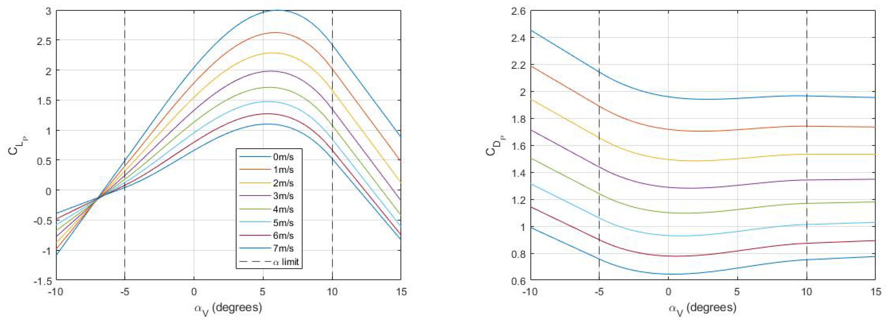This section denotes airspeed $V^a$ as V for simplicity. To compute aerodynamic coefficients at intermediate airspeeds, angles of attack, and control surface deflections, surface-fit raw experimental coefficient data was analyzed and plotted in Figure 4. Here, the x-axis represents vehicle angle of attack ${\alpha }_V$ for stability derivatives and normalized control surface deflection $\delta a/\delta e/\delta r$ for control derivatives. The y-axis shows airspeed while the z-axis shows the given coefficient value. Polynomial surface fits poly32 of third degree in x and second degree in y were used for each aerodynamic coefficient:

$$C_{\ast }=p_{00}+p_{10}x+p_{01}y+p_{20}{x}^2+p_{11}xy+p_{02}{y}^2+p_{30}{x}^3+p_{21}{x}^{2}y+p_{12}x{y}^2.$$

(21)

This formulation allows for convenient interpolation and extrapolation of data beyond the tested values. The poly32 fit with nine parameters captures the trends, well as shown in Figure 4, but does not overfit the data since we have 12 experimental data points for the stability derivatives and 15 data points for control derivatives from [14]. Derived polynomial coefficient parameters for all 3D surface fits in each flight mode are tabulated in

Table 3. Polynomial surface fit parameters for aerodynamic coefficients in all three QuadPlane flight modes.

Coeff.	${\mathit{p}}_{00}$	${\mathit{p}}_{10}$	${\mathit{p}}_{01}$	${\mathit{p}}_{20}$	${\mathit{p}}_{11}$	${\mathit{p}}_{02}$	${\mathit{p}}_{30}$	${\mathit{p}}_{21}$	${\mathit{p}}_{12}$
Plane Mode
$C_{L_P}$	$-7.68\times {10}^{-2}$	$3.07\times {10}^{-1}$	$5.34\times {10}^{-2}$	$-7.20\times {10}^{-3}$	$-2.26\times {10}^{-2}$	$-2.00\times {10}^{-3}$	$-1.40\times {10}^{-3}$	$9.29\times {10}^{-4}$	$7.44\times {10}^{-4}$
$C_{D_P}$	$1.88\times {10}^0$	$-3.08\times {10}^{-2}$	$-2.39\times {10}^{-1}$	$4.70\times {10}^{-3}$	$4.40\times {10}^{-3}$	$8.60\times {10}^{-3}$	$-1.89\times {10}^{-4}$	$-1.34\times {10}^{-4}$	$-1.16\times {10}^{-4}$
$C_{M_{\alpha }}$	$-1.74\times {10}^0$	$-5.75\times {10}^{-2}$	$2.71\times {10}^{-1}$	$-7.83\times {10}^{-4}$	$2.20\times {10}^{-3}$	$-1.00\times {10}^{-2}$	$-9.53\times {10}^{-5}$	$2.43\times {10}^{-4}$	$-1.03\times {10}^{-4}$
$C_{M_{{\delta }_e}}$	$8.3\times {10}^{-5}$	$4.47\times {10}^0$	$-5.70\times {10}^{-3}$	$2.98\times {10}^{-1}$	$-4.93\times {10}^{-1}$	$3.54\times {10}^{-4}$	$-4.91\times {10}^{-1}$	$-1.70\times {10}^{-2}$	$1.69\times {10}^{-2}$
$C_{r{m}_{{\delta }_a}}$	$-2.54\times {10}^{-2}$	$1.48\times {10}^0$	$-3.40\times {10}^{-3}$	$-6.11\times {10}^{-2}$	$-6.58\times {10}^{-2}$	$2.16\times {10}^{-4}$	$-4.30\times {10}^{-1}$	$2.40\times {10}^{-3}$	$1.70\times {10}^{-3}$
$C_{r{m}_{{\delta }_r}}$	$8.54\times {10}^{-2}$	$-8.33\times {10}^{-1}$	$-1.86\times {10}^{-2}$	$6.76\times {10}^{-2}$	$1.01\times {10}^{-1}$	$8.44\times {10}^{-4}$	$8.53\times {10}^{-2}$	$-4.60\times {10}^{-3}$	$-3.70\times {10}^{-3}$
$C_{y{m}_{{\delta }_a}}$	$1.30\times {10}^{-2}$	$-1.76\times {10}^{-1}$	$-2.70\times {10}^{-3}$	$-1.15\times {10}^{-2}$	$1.07\times {10}^{-2}$	$1.34\times {10}^{-4}$	$4.72\times {10}^{-2}$	$3.35\times {10}^{-4}$	$-4.44\times {10}^{-4}$
$C_{y{m}_{{\delta }_r}}$	$5.52\times {10}^{-2}$	$2.44\times {10}^0$	$-1.14\times {10}^{-2}$	$4.72\times {10}^{-2}$	$-2.88\times {10}^{-1}$	$5.48\times {10}^{-4}$	$-2.03\times {10}^{-1}$	$-4.90\times {10}^{-3}$	$1.01\times {10}^{-2}$
$C_{Y_{{\delta }_r}}$	$9.80\times {10}^{-3}$	$-8.04\times {10}^{-1}$	$-1.50\times {10}^{-3}$	$4.80\times {10}^{-3}$	$9.48\times {10}^{-2}$	$5.08\times {10}^{-5}$	$5.87\times {10}^{-2}$	$4.82\times {10}^{-4}$	$-3.30\times {10}^{-3}$
Quad Mode
$C_{L_P}$	$2.04\times {10}^0$	$2.74\times {10}^{-1}$	$-2.69\times {10}^{-1}$	$-1.26\times {10}^{-2}$	$-2.81\times {10}^{-2}$	$1.02\times {10}^{-2}$	$-1.10\times {10}^{-3}$	$1.30\times {10}^{-3}$	$1.10\times {10}^{-3}$
$C_{D_P}$	$1.96\times {10}^0$	$-1.48\times {10}^{-2}$	$-2.50\times {10}^{-1}$	$3.40\times {10}^{-2}$	$2.10\times {10}^{-3}$	$9.00\times {10}^{-3}$	$-1.85\times {10}^{-4}$	$-3.98\times {10}^{-5}$	$-4.09\times {10}^{-5}$
$C_{D_Q}$	$-2.50\times {10}^{-1}$	$3.40\times {10}^{-3}$	$4.67\times {10}^{-2}$	$-8.61\times {10}^{-4}$	$-1.20\times {10}^{-3}$	$-9.43\times {10}^{-4}$	$9.38\times {10}^{-6}$	$9.20\times {10}^{-5}$	$4.76\times {10}^{-5}$
$M_{\mathsf{\Delta }T}$	$0.00\times {10}^0$	$-7.80\times {10}^{-3}$	$2.07\times {10}^{-1}$	$4.50\times 10-3$	$8.50\times {10}^{-3}$	$-4.50\times {10}^{-3}$	$-4.95\times {10}^{-4}$	$-3.76\times {10}^{-4}$	$-1.84\times {10}^{-4}$
Hybrid Mode
$C_{L_P}$	$-6.24\times {10}^{-1}$	$1.99\times {10}^{-1}$	$1.05\times {10}^{-1}$	$1.65\times {10}^{-4}$	$-1.21\times {10}^{-2}$	$-3.00\times {10}^{-3}$	$-1.60\times {10}^{-3}$	$4.81\times {10}^{-4}$	$5.38\times {10}^{-4}$
$C_{D_P}$	$1.86\times {10}^0$	$-3.46\times {10}^{-2}$	$-2.37\times {10}^{-1}$	$4.50\times {10}^{-3}$	$4.40\times {10}^{-3}$	$8.50\times {10}^{-3}$	$-1.33\times {10}^{-4}$	$-1.51\times {10}^{-4}$	$-1.11\times {10}^{-4}$
$C_{D_Q}$	$7.86\times {10}^{-1}$	$1.30\times {10}^{-3}$	$-5.57\times {10}^{-2}$	$-5.23\times {10}^{-4}$	$-1.70\times {10}^{-3}$	$1.50\times {10}^{-3}$	$-3.22\times {10}^{-5}$	$5.32\times {10}^{-5}$	$7.50\times {10}^{-5}$
$M_{\mathsf{\Delta }T}$	$0.00\times {10}^0$	$2.00\times {10}^{-3}$	$2.02\times {10}^{-1}$	$2.80\times {10}^{-3}$	$7.40\times {10}^{-3}$	$-5.30\times {10}^3$	$-2.95\times {10}^{-4}$	$-2.94\times {10}^{-4}$	$-2.10\times {10}^{-4}$

. The coefficients $C_{M_{\alpha }}$ and $C_{Y_{{\delta }_r}}$ are common across all three flight modes; $C_{M_{{\delta }_e}}$, $C_{r{m}_{{\delta }_a}}$, $C_{r{m}_{{\delta }_r}}$, $C_{y{m}_{{\delta }_a}}$, and $C_{y{m}_{{\delta }_r}}$ are common among the Plane and Hybrid mode; and the remaining coefficients are unique to each referenced flight mode. Note that the coefficient of lift $C_{L_P}$ for each flight mode is modeled as a cubic function of ${\alpha }_V$ to additionally capture wing stall and post-stall behavior. $C_{D_P}$ as a function of ${\alpha }_V$ is predominantly quadratic, so the corresponding cubic fit parameter $p_{30}$ is negligible for all three flight modes per Table 3. All control derivatives show linear dependence on control surface deflection.

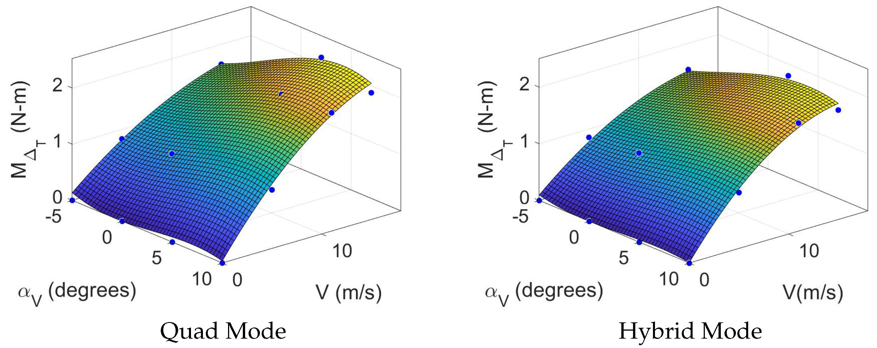
$M_{\mathsf{\Delta }T}$ is a unique stability derivative for Quad and Hybrid modes, analogous to $C_{M_{\alpha }}$ for aircraft. This parameter represents the pitching moment from vertical propulsion as a function of V and ${\alpha }_V$ and differs in that it is not scaled by airspeed (V) but instead represents direct pitching moment application arising from differential thrust from front and rear vertical propulsors while there is airflow along the body x-axis as described in [14]. $M_{\mathsf{\Delta }T}$ is zero at zero airspeed. Therefore, four additional data points are added to the data from [14] where $M_{\mathsf{\Delta }T}=0$ at each tested ${\alpha }_V$ value, as shown in Figure 5. This moment becomes zero as the vertical propulsors stop spinning, so we implement this moment in simulation as a total thrust reduction in $\mathsf{\Delta }T=2M_{\mathsf{\Delta }T}/L_Q$ for the rear vertical motors. For each rear motor, thrust is reduced by $\mathsf{\Delta }T/2$.

For full multi-mode flight simulation, we require data outside of the experimentally acquired values, especially for operating at 0 m/s $\le V\le$ 5 m/s in Quad mode. As most aerodynamic coefficients are scaled by $V^2$, we must extrapolate surface fits to compute values down to V = 0 m/s. The maximum achievable QuadPlane airspeed of $V=17$ m/s is set as the upper limit for extrapolation. We also extrapolate normalized control surface deflections ${\delta }_e/{\delta }_a/{\delta }_r$ to support a normalized range of values between $-1$ and 1.

Table 4. QuadPlane flight envelope limits used in simulations for all flight modes.

Flight Mode	${\mathit{V}}^{\mathit{a}}$ (m/s)	${\mathit{T}}_1/{\mathit{T}}_2/{\mathit{T}}_3/{\mathit{T}}_4$ (N)	${\mathit{T}}_{\mathit{fwd}}$ (N)	${\mathit{\delta }}_{\mathit{e}}/{\mathit{\delta }}_{\mathit{a}}/{\mathit{\delta }}_{\mathit{r}}$	$\mathit{\beta }$
Quad	0 to $6.5$	0 to $F_{max}^v(V,{\alpha }_V-{90}^{\circ })$	0	0	$-5^{\circ }$ to $5^{\circ }$
Hybrid	$0.5$ to 13	0 to $F_{max}^v(V,{\alpha }_V-{90}^{\circ })$	0 to $F_{max}^f(V,{\alpha }_V)$	$-1$ to 1	$-5^{\circ }$ to $5^{\circ }$
Plane	12 to 17	0	0 to $F_{max}^f(V,{\alpha }_V)$	$-1$ to 1	$-5^{\circ }$ to $5^{\circ }$

lists airspeed, thrust, sideslip, and normalized control surface deflection limits across all three flight modes for all simulation studies in this paper.

The ${\alpha }_V$ range over which aerodynamic data is available [$-5^{\circ },{10}^{\circ }$] is also restrictive for real-world flight conditions, especially in Quad mode. For instance, as can be seen in Section 7.3, for the QuadPlane to fly at an airspeed of 5 m/s in Quad mode, an ${\alpha }_V$ of nearly $-{10}^{\circ }$ is required. To extrapolate ${\alpha }_V$ values, a tangent is generated on the 2D curve derived by splicing the 3D fit surface at a given V with the value of the coefficient on the tangent at the desired ${\alpha }_V$. Figure 6 shows the resulting extrapolation. Note that we do not have any aerodynamic data for vertical flight, so we assume aerodynamic forces are negligible for $V\le$ 1 m/s when ${\alpha }_V>{45}^{\circ }$ or ${\alpha }_V<-{45}^{\circ }$ and restrict vertical speed in all simulations to less than 1 m/s.

Aerodynamic forces and moments can be calculated from aerodynamic coefficients in the wind frame for a given flight mode. However, the experimental data in [13] is only available for $\beta =0$. Instead of ignoring forces and moments in the presence of crosswinds, we use the dimensions of the vertical stabilizer and approximate it as a finite wing with chord $c_{vs}$ and area $S_{vs}$ with a NACA 0006 airfoil [50]. NACA data is used to define aerodynamic coefficient of lift $C_{L_{vs}}$ and pitching moment $C_{M_{vs}}$ for the vertical stabilizer as described previously in [12]. We then compute the lift and pitching moment on the vertical stabilizer for a given sideslip angle. Note that the angle of attack for the vertical stabilizer is the sideslip angle for the aircraft. The net aerodynamic forces and moments on the aircraft in the wind frame are then given by

$$\begin{array}{cccc}{\overrightarrow{F}}_{A|w}=\left[\begin{array}{c}{F}_{x_A}\\ F_{y_A}\\ F_{z_A}\end{array}\right]& \hfill =\left[\begin{array}{c}-\overline{q}{C}_{D_P}S-C_{D_Q}V\\ \overline{q}{C}_{Y_{{\delta }_r}}S+\overline{q}{C}_{L_{vs}}{S}_{vs}\\ -\overline{q}{C}_{L_P}S\end{array}\right],\hfill & \hfill {\overrightarrow{M}}_{A|w}=\left[\begin{array}{c}{M}_{x_A}\\ M_{y_A}\\ M_{z_A}\end{array}\right]& \hfill =\left[\begin{array}{c}\overline{q}cS(C_{r{m}_{{\delta }_a}}+C_{r{m}_{{\delta }_r}})\\ \overline{q}cS(C_{M_{\alpha }}+C_{M_{{\delta }_e}})+M_{\mathsf{\Delta }T}\\ \overline{q}cS(C_{y{m}_{{\delta }_a}}+C_{y{m}_{{\delta }_r}})+\overline{q}{c}_{vs}{S}_{vs}{C}_{M_{vs}}\end{array}\right],\hfill \\ \hfill {\overrightarrow{F}}_{A|b}& ={}^B\mathbf{R}_w\ast {\overrightarrow{F}}_{A|w},\hfill & \hfill {\overrightarrow{M}}_{A|b}& ={}^B\mathbf{R}_w\ast {\overrightarrow{M}}_{A|w},\hfill \end{array}$$

(22)

where $\overline{q}={\displaystyle \frac{1}{2}}\rho V^2$ denotes the dynamic pressure, and coefficients $C_{L_{vs}}$, $C_{M_{vs}}$ are derived from NACA data. Based on the flight mode, aerodynamic coefficient values are computed for the remaining terms in Equation (22) to estimate net aerodynamic forces and moments. Forces and moments were then rotated from wind to body frame with ${}^B\mathbf{R}_w$ to apply body frame dynamics from Equation (1). Note that the stall speed for the QuadPlane was determined to be 11.9 m/s using the aerodynamic model for Plane mode.

7.2. Propulsion Model

The QuadPlane experiences forces $F_T$ and moments $M_T$ from its four vertical thrusters and one forward thrust module:

$$\begin{array}{ccc}\hfill {\overrightarrow{F}}_T=\left[\begin{array}{c}{T}_{fwd}\\ 0\\ T_1+T_2+T_3+T_4\end{array}\right],& \hfill \hfill & \hfill {\overrightarrow{M}}_T=\left[\begin{array}{c}{L}_Q/2\ast (-T_1-T_2+T_3+T_4)+{\gamma }_f\ast T_{fwd}\\ L_Q/2\ast (T_1-T_2-T_3+T_4)\\ {\gamma }_v\ast (T_1-T_2+T_3-T_4)\end{array}\right],\end{array}$$

(23)

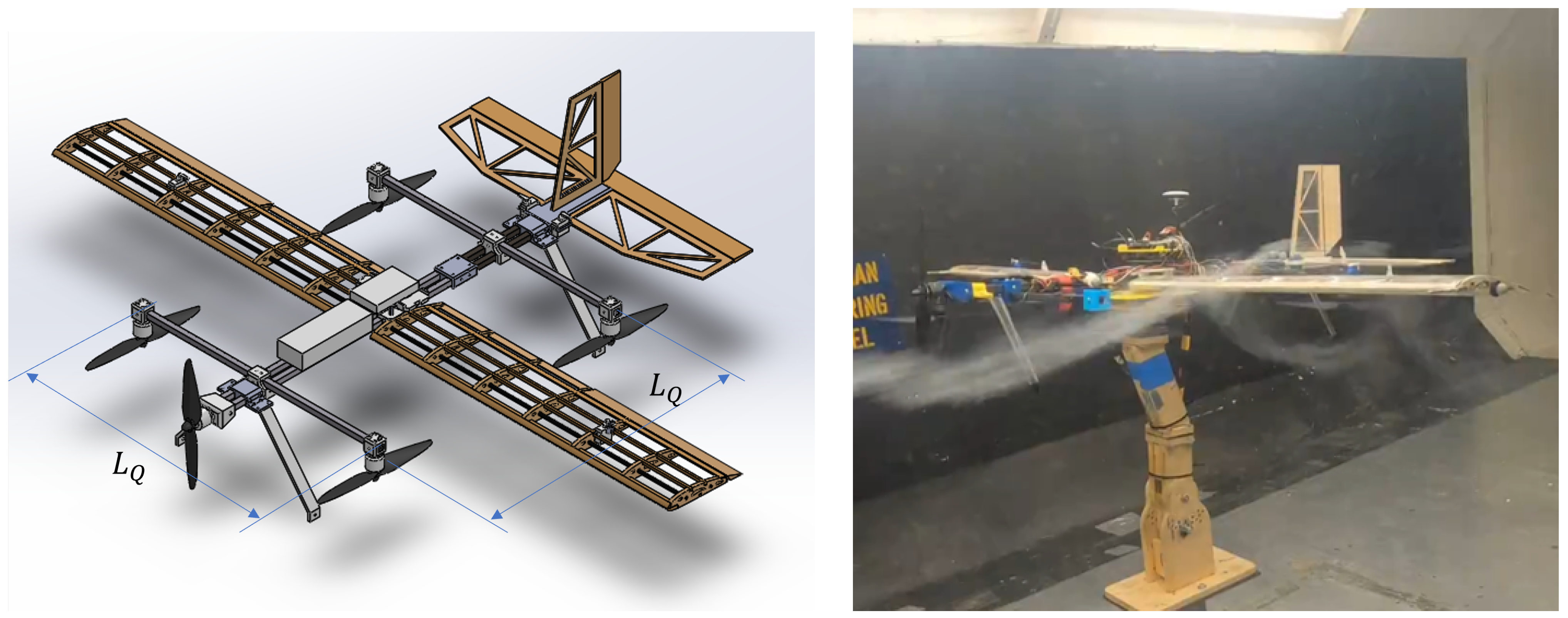
where ${\gamma }_f$ and ${\gamma }_v$ are torque coefficients for the forward and vertical thrust modules, respectively, and $L_Q$ is the length of the quadrotor square [21]. Together with Equation (22), the total force and moment on the aircraft in the body frame can be computed and used in Equation (1) to propagate the aircraft state. In Quad mode, $T_{fwd}=0$ as the forward thrust module is inactive, while in Plane mode, $T_1=T_2=T_3=T_4=0$ since the vertical thrusters are inactive.

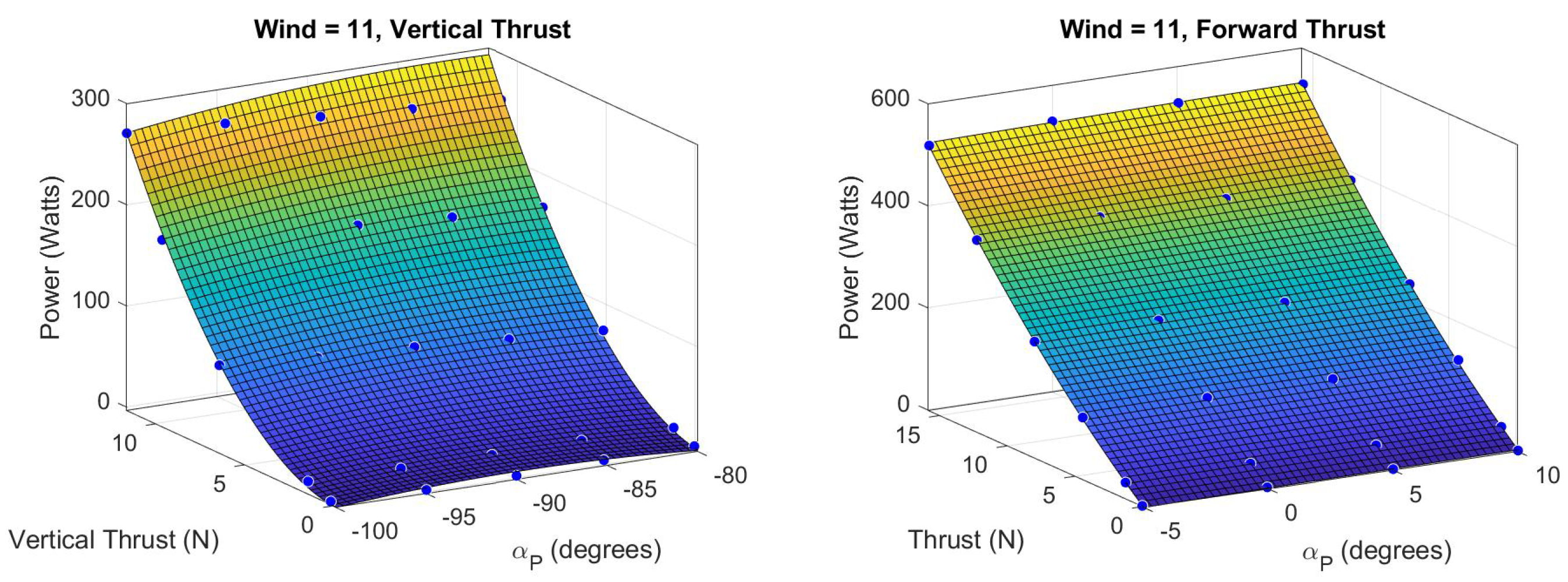
Propulsion system test data from [14] was used to derive a 3D surface mapping between the propeller angle of attack ${\alpha }_p$, thrust force, and power consumption over the four test airspeeds (V = 0, 5, 11, 15 m/s) for both vertical and forward thrust modules. The propeller angle of attack for the front motor is the same as the aircraft angle of attack (${\alpha }_p={\alpha }_V$) and is offset by ${90}^{\circ }$ for the vertical motors (${\alpha }_p={\alpha }_V-{90}^{\circ }$). The thrust from the forward thrust module used in [13,14] was found to be insufficient to overcome drag and maintain steady level flight at airspeeds greater than 11 m/s, maxing out at $4N$ at 15 m/s. A new, more powerful E-flite Power 25 motor and a larger ${11}^{″}\times 8^{″}$ propeller were installed, and propulsion tests were repeated using the methods from [14]. Surface fits for vertical and forward thrust modules at test airspeed V = 11 m/s are shown in Figure 7. For any desired thrust, power consumption is derived with linear interpolation from the two closest test airspeeds.

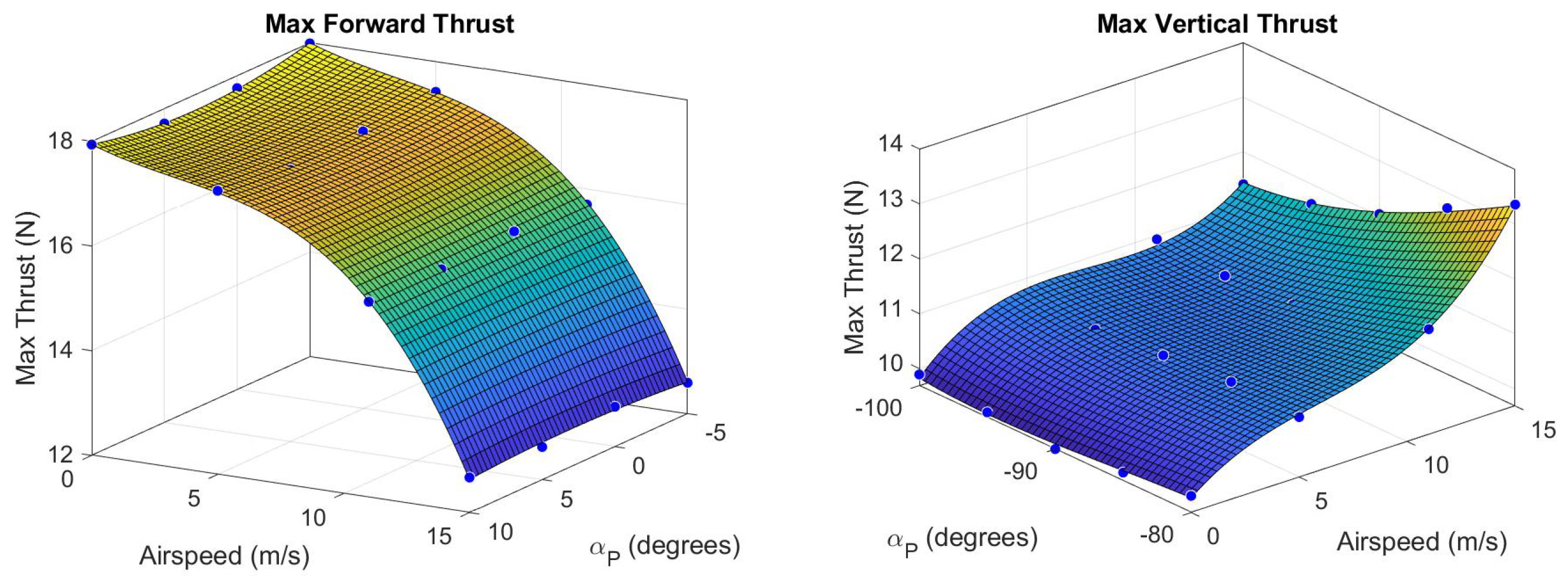
Maximum vertical thrust $F_{max}^v$ and forward thrust $F_{max}^f$ were determined as a function of V and ${\alpha }_p$ and are shown in Figure 8. These surfaces define commanded thrust saturation limits in simulation. Notice the drop in maximum forward thrust at higher airspeeds due to increased propeller drag and weathervaning. Note also an increase in vertical thrust, especially for ${\alpha }_p\ge -{90}^{\circ }$, as propeller thrust becomes aligned with propeller drag.

7.3. Trim States

Trim states are equilibrium aircraft configurations useful for steady state flight and control design. The nonlinear system of equations governing aircraft dynamics can be linearized about a trim state such that the derived linear system is a close approximation of the dynamics within the region of attraction. Computation of trim states for the QuadPlane across all flight modes is described here. Trim and propulsion models in turn support power consumption, range, and endurance estimation.

A lookup table for trim state solutions in each flight mode M over an achievable airspeed range was constructed. This table provides the trim state (${\overrightarrow{X}}_{trim}$) and corresponding control vectors (${\overrightarrow{u}}_{Q_{trim}},{\overrightarrow{u}}_{P_{trim}}$) for a given cruise airspeed. For Hybrid mode, an additional entry for trim pitch angle ${\theta }_{d_{trim}}$ is provided. To derive the trim state for each airspeed in the lookup table, a distinct cost function is defined for each flight mode as described in the following paragraphs. The MATLAB R2024a $fmincon\left(\right)$ function is then used with a Sequential Quadratic Programming (SQP) algorithm to minimize the cost function within a step tolerance of ${10}^{-16}$ and constraint tolerance of ${10}^{-6}$. Bounds and constraints for steady level flight trim states are listed in

Table 5. Limits on state and control variables used to define the steady level QuadPlane trim state lookup table.

Flight Mode	Bounds	Constraints
Q, P & H		$v=0$; $\psi =0$; $\theta =ta{n}^{-1}\left({\displaystyle \frac{u}{w}}\right)$;
	$-5^{\circ }\le \varphi \le 5^{\circ }$;	$\sqrt{{\dot{x}}^2+{\dot{y}}^2+{\dot{z}}^2}=V$;
	$-1^{\circ }\le \beta =si{n}^{-1}\left({\displaystyle \frac{v}{(u^2+v^2+w^2)}}\right)\le 1^{\circ }$	$\dot{z}=0$; $\dot{u}=\dot{v}=\dot{w}=0$;
		$\dot{p}=\dot{q}=\dot{r}=0$
Q	${\alpha }_V\le 5^{\circ }$;	${\delta }_a^A={\delta }_e^A={\delta }_r^A=T_{fwd}=0$
	$0\le T_i\le F_{v_{max}}(V,{\alpha }_V)$$\forall i\in \{1,2,3,4\}$
P	$-{30}^{\circ }\le {\delta }_a^A\le {30}^{\circ }$; $-{30}^{\circ }\le {\delta }_e^A\le {30}^{\circ }$;	$T_i=0$$\forall i\in \{1,2,3,4\}$
	$-{40}^{\circ }\le {\delta }_r^A\le {40}^{\circ }$;
	$0\le T_{fwd}\le F_{fw{d}_{max}}(V,{\alpha }_V)$
H	$-{30}^{\circ }\le {\delta }_a^A\le {30}^{\circ }$; $-{30}^{\circ }\le {\delta }_e^A\le {30}^{\circ }$;	$\theta ={\theta }_d$
	$-{40}^{\circ }\le {\delta }_r^A\le {40}^{\circ }$;
	$0\le T_i\le F_{v_{max}}(V,{\alpha }_V)$$\forall i\in \{1,2,3,4\}$;
	$0\le T_{fwd}\le F_{fw{d}_{max}}(V,{\alpha }_V)$; ${\alpha }_V\le 5^{\circ }$

. Note that ${\delta }_a^A,{\delta }_e^A,{\delta }_r^A$ denote the angular aileron, elevator and rudder deflections respectively.

In Quad mode, a trivial trim state for hover (V = 0 m/s) can be obtained by simple force balance with zero pitch and roll, where aircraft weight is equally distributed across the four vertical thrust motors. The aircraft must maintain a negative trim pitch angle for level flight at a given airspeed to counter drag. Determining Quad mode trim pitch angles across operational airspeeds is crucial for the design of $Q2P$ and $P2Q$ transition controllers to enable smooth pitch tracking over transitions. The cost function for Quad mode penalizes vertical thrust and is given below with $diag\left(\right)$ defining a diagonal 4 × 4 matrix:

$$\begin{array}{ccc}\hfill Cos{t}_Q& \hfill ={\overrightarrow{u}}_Q^T\ast {\mathbf{Q}}_Q\ast {\overrightarrow{u}}_Q,\hfill & \hfill {\mathbf{Q}}_Q=diag(100,100,100,100).\end{array}$$

(24)

In Plane mode, forward thrust and elevator deflection govern the trim pitch angle for the aircraft at a given airspeed. The cost function for Plane mode penalizes vertical velocity $\overrightarrow{\dot{X}}\left(3\right)$, translational accelerations $\overrightarrow{\dot{X}}(4,5,6)$, rotational velocities $\overrightarrow{\dot{X}}(7,8,9)$ and rotational accelerations $\overrightarrow{\dot{X}}(10,11,12)$, in addition to the forward thrust $T_{fwd}$. Cost is defined below; note that the cost penalty for forward thrust is large to minimize power consumption for each trim state.

$$\begin{array}{cccc}\hfill & \hfill \hfill & & \hfill Cos{t}_P={\overrightarrow{\dot{X}}}^{\top }\ast {\mathbf{Q}}_P\ast \overrightarrow{\dot{X}}+T_{fwd}\ast {\mathbf{R}}_P\ast T_{fwd},\hfill \\ \hfill {\mathbf{R}}_P& =100000,\hfill & \hfill {\mathbf{Q}}_P=& diag(0,0,10000,100,100,100,1000,1000,1000,100,100,100).\hfill \end{array}$$

(25)

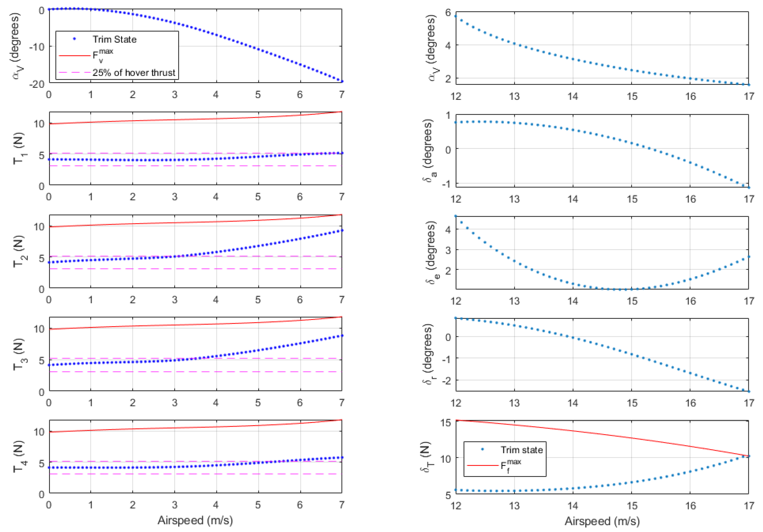
Figure 9 shows trim control inputs and pitch angle as a function of airspeed for Quad mode (left) and Plane mode (right). Dashed pink lines show a $25\%$ thrust band around the vertical hover thrust, while solid red lines show maximum thrust at the given airspeed and pitch angle. The trim pitch angle is equivalent to ${\alpha }_V$ for steady-level flight. Quad mode trim pitch becomes increasingly negative for higher airspeeds. Vertical thrust trends are as expected for forward flight in Quad mode with negative pitch angles. The QuadPlane has a sufficient safety margin between the required and maximum vertical thrust at the Quad mode airspeed limit of 7 m/s. In Plane mode, the required forward thrust increases with increasing airspeed, as expected. Plane mode trim states require slight deflections of the aileron and rudder to balance the p-factor rolling moment generated by the forward thrust module. At an airspeed of 16.9 m/s, the forward thrust required approaches the maximum thrust line, i.e., the maximum achievable trim airspeed for the aircraft is 16.9 m/s. As expected, the angle of attack at lower airspeeds is higher to maximize lift and drops as airspeed increases to reduce drag as forward thrust becomes the limiting factor.

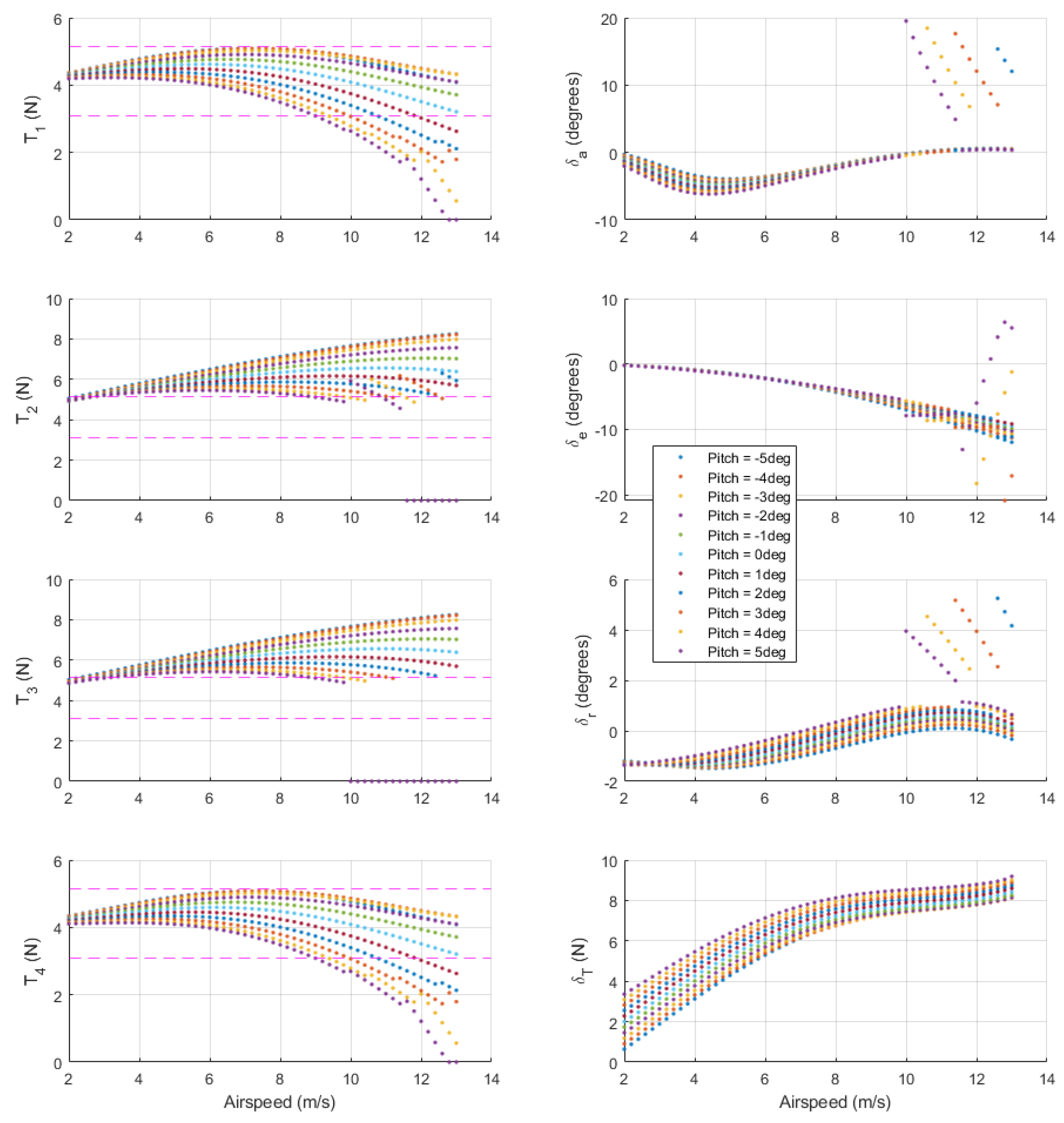
The cost function for Hybrid mode penalizes all thrust values, with a relatively low penalty for forward thrust to encourage acceleration to Plane speed. The cost penalty for elevator deflection is set high to prevent saturation, offloading most of the pitching moment compensation to differential vertical thrust. Hybrid mode trim states are computed across a range of feasible pitch angles.

$$Cos{t}_H={\overrightarrow{T}}_{cost}^{\top }\ast {\mathbf{Q}}_H\ast {\overrightarrow{T}}_{cost}+{\overrightarrow{C}}_{cost}^{\top }\ast {\mathbf{R}}_H\ast {\overrightarrow{C}}_{cost},$$

(26)

$$\begin{array}{ccc}\hfill {\overrightarrow{T}}_{cost}={\left[\begin{array}{ccccc}{T}_1& T_2& T_3& T_4& T_{fwd}\end{array}\right]}^T,& \hfill \hfill & \hfill {\overrightarrow{C}}_{cost}={\left[\begin{array}{cccccc}{F}_v& {\tau }_x& {\tau }_z& {\delta }_a& {\delta }_e& {\delta }_r\end{array}\right]}^T,\\ \hfill {\mathbf{Q}}_H=diag(10000,10000,10000,10000,100),& \hfill \hfill & \hfill {\mathbf{R}}_H=diag(1000,50,50,5000,1000000,5000).\end{array}$$

Figure 10 shows trim states for the QuadPlane as a function of airspeed across pitch angles of $-5^{\circ }$ to $5^{\circ }$ in $1^{\circ }$ increments. This range was selected to cover Quad trim pitch angles up to airspeeds of 3.5 m/s and Plane mode trim pitch angles. Forward thrust increases with airspeed, as expected. At Plane mode cruise airspeed of 12.5 m/s, a forward thrust of $8-9N$ is required to maintain trim flight in Hybrid mode as opposed to $5.5N$ in Plane mode, as seen in Figure 9. This excess forward thrust is required to counter the excess drag created by the spinning vertical thrust propellers in Hybrid mode. Notice that thrust from rear left motor $T_3$ drops to zero beyond airspeeds of 10 m/s for ${\theta }_d=5^{\circ }$, 10.5 m/s for ${\theta }_d=4^{\circ }$, 11 m/s for ${\theta }_d=3^{\circ }$, and 12 m/s for ${\theta }_d=2^{\circ }$. This occurs because wing lift increasingly supports weight as airspeed and pitch angle increase. The rear left motor turns off first due to a p-factor rolling moment from the front motor. Once $T_3=0$, step changes in the remaining control inputs are required to stabilize the aircraft and maintain trim flight. In summary, Hybrid mode offers the largest operating envelope using any combination of airspeed and pitch angle in Figure 10.

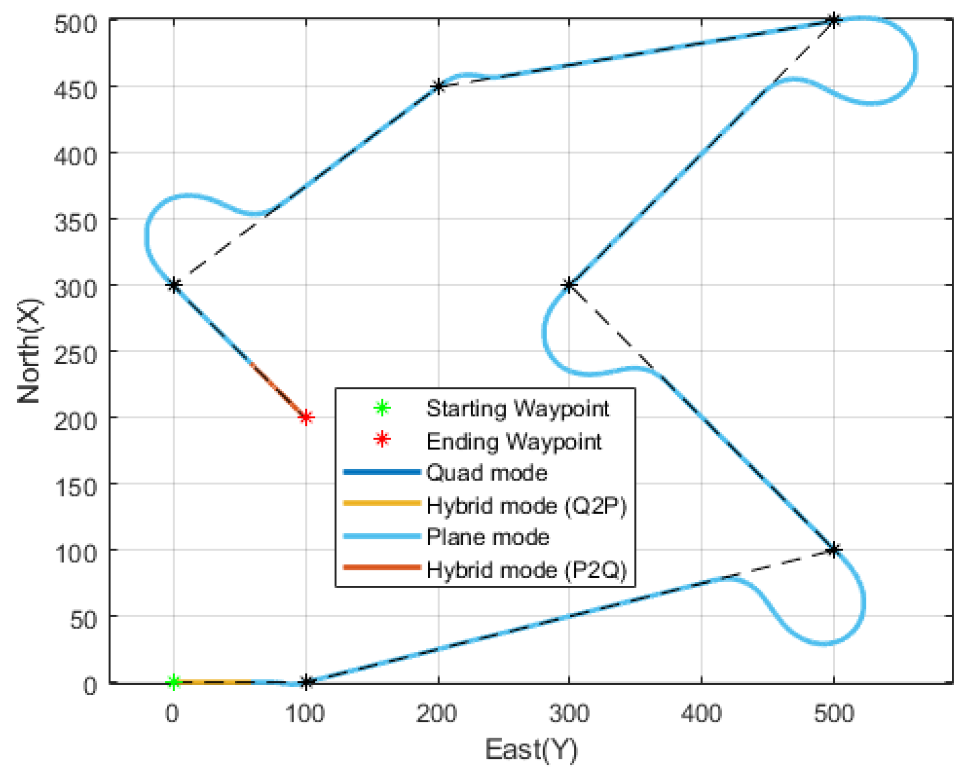
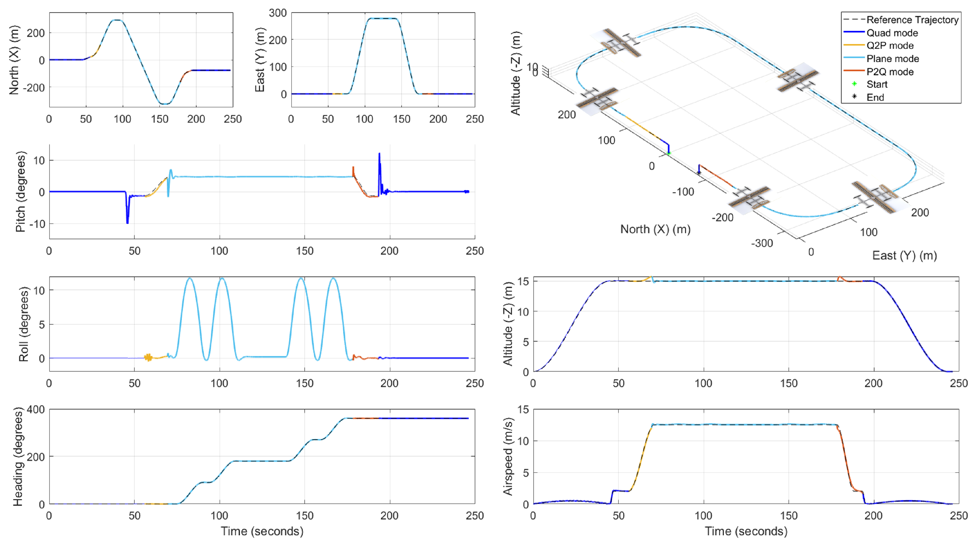
7.4. Transition Trajectories

QuadPlane Hybrid mode activates to assure stability when accelerating from Quad to Plane mode or vice versa. A $Q2P$ transition follows a cubic spline in airspeed from hover to the best cruise airspeed for the QuadPlane $V^a$ = 12.5 m/s (as seen in Section 8.1) over time $t_{Q2P}$, subject to $a_{max}^a$ = 2 m/s² with zero initial and final acceleration. Flight mode M changes from Quad to Hybrid to Plane mode over the transition per Equation (5), where $V_{QH}$ = 2 m/s and $V_{HP}$ = 12 m/s. Pitch angle time history ${\overrightarrow{\theta }}_d\left(t\right)$ also follows a cubic spline from Quad trim pitch angle at hover to the Plane trim pitch angle at $V^a$ = 12.5 m/s over the same transition time $t_{Q2P}$, with zero initial and final pitch rate. After a $Q2P$ transition, the remaining segment is flown in Plane mode at the best cruise airspeed $V^a$ = 12.5 m/s. The reverse happens over a $P2Q$ transition at a higher deceleration, $a_{max}^a=-2.5$ m/s², and a shorter time $t_{P2Q}$. $Q2P$ transitions occur at the start of the segment, while $P2Q$ transitions occur towards the end of the segment to minimize total energy consumption by maximizing time spent in Plane mode.

8. Simulation Results

This section presents QuadPlane performance and simulation results. QuadPlane range and endurance for steady level flight are first presented along with trim state power consumption for cruise, turning, climbing, and descending flight over representative airspeeds across the three flight modes. Next, trajectory tracking results are presented in each flight mode with and without ambient wind. A full flight case study from take-off to landing is presented. Results from EAC flight planning are presented, including sensitivity and Pareto analyses, as well as a comparison with $FOD$ plans.

8.1. Range, Endurance, and Power Consumption

The power required to maintain trim states derived in Section 7.3 is computed using the propulsion model from Section 7.2. QuadPlane power consumption P is plotted in Figure 11 for maintaining steady level flight in Quad and Plane mode. As expected, Plane mode is more power efficient than Quad mode. Plane mode uses $69.6\%$ of hover power in cruise at 12.5 m/s and is most power efficient close to stall speed. Therefore, it is $30.4\%$ more efficient for the QuadPlane to loiter in Plane mode than to hover in Quad mode. In general, more power is consumed at higher airspeeds as expected, yet this alone does not provide sufficient insight into total energy consumption. Define Energy per Distance as $\mathcal{F}=P/V$. $\mathcal{F}$ provides a distance-normalized measure of energy consumed over a flight at constant airspeed V. As seen in Figure 11, $\mathcal{F}$ increases with airspeed in Plane mode but decreases with airspeed in Quad mode. The most efficient $\mathcal{F}$ is Plane mode at $V^a=12.5$ m/s, defined as the optimal QuadPlane cruise airspeed.

Figure 12 shows Hybrid mode power consumption over airspeeds ranging from 2 m/s to 13 m/s, bridging the gap between Quad and Plane mode airspeed ranges. Hybrid mode consumes higher power than Quad mode at the same airspeed because of the additional forward thrust required to maintain a desired pitch angle. With an increase in airspeed and higher forward thrust, vertical thrust and required power smoothly decrease as wing lift offsets aircraft weight.

The sharp dips in Figure 12 correspond to a left rear vertical thrust command of zero. For pitch angles greater than $3^{\circ }$, we see a second dip at even higher airspeeds, indicating a second vertical thrust motor has shut off. The below simulations command pitch to follow a smooth profile connecting Quad and Plane pitch angles as described in Section 7.4.

Range is the maximum distance the aircraft can travel, and endurance is the maximum time of flight. Each is defined for straight and level trim state flight that uses $85\%$ of the QuadPlane’s total battery capacity. Endurance depends strictly on power consumption, while range depends on energy per distance $\mathcal{F}$. The QuadPlane is powered by a 4S Lithium Polymer ($LiPo$) battery with a capacity of 2200 mAh or 32.56 Wh. Per Figure 13, the highest endurance of 547.25 s occurs in Plane mode at an airspeed of 12 m/s. The highest range of 6.61 km occurs at a slightly greater airspeed of 12.5 m/s, also in Plane mode. In Quad mode, the highest endurance is seen while hovering. As expected, the lowest range and endurance values occur in Hybrid mode. Based on the mission, different values of pitch angles can be held while operating in Hybrid mode; higher pitch angles yield higher range and endurance. $\mathcal{F}$ across the three flight modes is plotted in Figure 14 with Hybrid mode data for desired pitch ${\theta }_d=0^{\circ }$. As shown, Quad mode is most efficient under airspeeds of 6.5 m/s. Hybrid mode is then required up to the Plane mode stall speed of 12 m/s, beyond which Plane mode is most efficient.

Table 6. QuadPlane power consumption (P) and Energy per distance $\mathcal{F}$ in cruise and turning flight across all flight modes.

V (m/s)	Cruise	$\mathit{\varphi }{(}^{\circ })$	$\mathit{\theta }{(}^{\circ })$	P (W)	$\mathcal{F}$ (J/m)	Turn	$\dot{\mathit{\sigma }}{(}^{\circ }/\mathit{s})$	$\mathit{\varphi }{(}^{\circ })$	$\mathit{\theta }{(}^{\circ })$	P (W)	$\mathcal{F}$ (J/m)
2	$Q^{\ast }$	0.0	−1.3	278	139	$Q^t$	50	10.1	−1.3	284	142
4		0.0	−7.0	318	80		50	19.7	−6.1	338	84
6		0.0	−15.0	427	71		50	28.7	−11.7	466	78
6	$H^{\ast }$	−0.1	0.0	478	80	$H^t$	20	12.5	0.0	514	64
8		−0.1	0.0	518	65		12	9.6	0.0	528	43
10		0.1	0.0	528	53		8	7.7	0.0	550	33
12		0.1	0.0	531	44		7	7.9	0.0	573	26
12	$P^{\ast }$	0.2	5.7	180	15	$P^t$	14	16.9	6.4	194	16
12.5		0.2	4.7	189	15		24	28.4	5.7	213	17
14		0.0	3.1	233	17		30	36.9	3.7	259	18
16		−0.5	2.0	369	23		30	40.2	2.4	395	25

lists cruise airspeeds (V) and corresponding maximum turn rates ($\dot{\sigma }$) that the QuadPlane can sustain in all three flight modes. Roll and pitch angles over cruise and turning trim states are shown along with power consumption and $\mathcal{F}$. Least power is consumed in Plane mode near the stall speed. For Hybrid mode, ${\theta }_d=0^{\circ }$ for all presented cruise and turning trim states. The QuadPlane is the most maneuverable and supports the highest turn rate in Quad mode and is the least maneuverable in Hybrid mode. Because Hybrid mode is least efficient and offers less maneuverability than Quad mode, Hybrid mode is used only under the following conditions for our simulations: (i) Transitions between Quad mode and Plane mode or vice versa; (ii) Sustained operations are desired at airspeeds between maximum Quad mode speed (7 m/s) and Plane mode stall speed (11.9 m/s), or (iii) the mission requires the QuadPlane to maintain a desired pitch angle while also tracking a trajectory at a given airspeed.

Table 7. Power consumption P and energy per distance $\mathcal{F}$ as a function of airspeed, climb and descent rates across all flight modes.

V (m/s)	Climb	$\dot{\mathit{z}}$ (m/s)	$\mathit{\theta }{(}^{\circ })$	P (W)	$\mathcal{F}$ (J/m)	Descent	$\dot{\mathit{z}}$ (m/s)	$\mathit{\theta }{(}^{\circ })$	P (W)	$\mathcal{F}$ (J/m)
2	$Q^c$	1.5	7.0	640	320	$Q^d$	−1.5	−7.5	237	119
4		2	0.8	619	155		−2	−9.2	343	86
6		2	−8.2	688	115		−2	−9.6	257	43
6	$H^c$	2	0.0	714	70	$H^d$	−0.8	0.0	413	47
8		2	0.0	767	50		−1	0.0	410	30
10		2.0	0.0	791	38		−1.2	0.0	370	17
12		1.3	0.0	753	34		−1.3	0.0	340	9
12	$P^c$	4	24.1	360	30	$P^d$	−3	−8.9	50	4
12.5		6	32.2	454	36		−4	−14.2	16	1
14		6	27.9	485	35		−4	−13.6	62	4
16		3	12.7	495	31		−7	−24.3	48.6	3

lists the pitch, power, and energy per distance data at representative airspeeds for maximum climb and descent rates supported in each flight mode. As expected, descending at a high rate in Plane mode yields the best $\mathcal{F}$ since the aircraft is able to use potential energy to counter aerodynamic drag. Near its maximum operational airspeed, Plane mode supports the highest descent rate but the lowest climb rate, as very little additional forward thrust is available at this airspeed. In Quad mode, climbing at 1.5 m/s while maintaining an airspeed of 2 m/s requires the QuadPlane to pitch up by $7^{\circ }$, much higher than the cruise trim pitch angle of $-1.3^{\circ }$. Climbing at 2 m/s in Quad mode while maintaining an airspeed of 6 m/s requires a pitch angle of $-8.2^{\circ }$, again much larger than the cruise trim pitch angle of $-{15}^{\circ }$.

8.2. Trajectory Tracking Results

QuadPlane guidance and tracking control are analyzed in simulated trajectories with and without ambient wind for all three flight modes. The sideslip angle is maintained within bounds per Table 5. All simulations have the aircraft pointed into the relative wind while tracking the desired ground trajectory. In Quad mode, constant ground speed is commanded while airspeed varies to handle wind. In Plane and Hybrid modes, constant airspeed is commanded while the ground speed changes according to the wind magnitude. The trajectories are generated per Section 4.3, and a time step $dt$ = 0.005 s is used for all simulations.

8.2.1. Quad Mode

Ambient wind velocity is constrained in Quad mode based on the desired ground velocity as described in [15]. Quad mode flight is simulated first in no wind, then in the wind speeds higher than commanded ground speed over square trajectories with Fly Coverage $FC$ and Hover $HV$ waypoints. The impact of carrot step $n_c$ was also studied with a small $n_c=1$ (time equivalent of 0.005 s) chosen based on observed tracking accuracy.

Figure 15 shows the QuadPlane in Quad mode, tracking the generated trajectory over the three cases. In all three cases, a ground cruise speed $V_c^g$ of 2 m/s is commanded. The mission is completed at the same time for the first two cases with and without ambient wind, as the aircraft acquires higher airspeed in the upwind sections and lower airspeed in the downwind section to compensate for the wind and maintain ground speed. Interestingly, the QuadPlane flies “backwards” in the ground frame, with heading offset by ${180}^{\circ }$ from the course angle at a cruise airspeed $V_c^a$ of 2 m/s in the downwind section of the trajectory, given wind speed $V^w$ of 4 m/s. This occurs as a result of always pointing into the relative wind direction and commanding ground speed slower than wind speed along the wind direction.

8.2.2. Plane Mode

Figure 16 shows results from three trajectory tracking simulations in ambient wind magnitudes $V^w$ of 0 m/s, 6 m/s, and 10 m/s, respectively, with the first two being square Fly-Coverage $FC$ and the third being Fly-Over Dubins $FOD$ trajectories. For simulating only Plane mode flight, we assume cruise flight at airspeed $V_c^a$ = 12.5 m/s as initial conditions, while the start and end waypoint type is set to $FC$. The desired airspeed is computed at each time step per Plane mode guidance described in Section 6.1. As the trajectory is generated for constant airspeed and ground speed varies per Equation (3), it takes the aircraft almost twice as long to complete the second trajectory as compared with the first one, even though the waypoints for both are the same. The second case features a curious turn at the end of the second segment, a natural result of the two-part cubic spline used for Fly-Coverage waypoints in the presence of a crosswind. The aircraft crabs into the wind by about ${30}^{\circ }$ along the crosswind section, maintaining a heading of $61.2^{\circ }$. Heading required at the end of the second segment is ${180}^{\circ }$ as the third segment points directly to the South. The $FC$ turn thus involves a sharp left turn into the wind followed by a right turn to align with the desired ground track. Since the turn follows two cubic splines in the desired heading ${\sigma }_d$, it is tracked smoothly despite its aggressive appearance in the ground track plot.

Figure 16c shows a holding pattern $FOD$ trajectory generated for ambient wind with $V^w$ = 10 m/s and ${\sigma }^w={180}^{\circ }$. Plane mode handles trajectory tracking in such high wind speeds, with a ground speed of 2.5 m/s in a headwind and 22.5 m/s in a tailwind. As expected, the ground track over smooth heading change cubic spline turns is significantly impacted by the wind. Carrot time steps for heading $n_{\sigma }=200$, and airspeed $n_V=200$ were used for $V^w\le$ 8 m/s, while $n_{\sigma }=250$ and $n_V=250$ were chosen otherwise to maintain a balance between control robustness and trajectory tracking accuracy.

8.2.3. Hybrid Mode

Figure 17 shows trajectory tracking simulation results at a cruise airspeed $V_c^a$ = 8 m/s in Hybrid mode over a square Fly-Coverage $FC$ trajectory and a Holding-Pattern Fly-Over Dubins $FOD$ trajectory with and without ambient wind. Similar to Plane mode, to ensure Hybrid mode operations over the entire trajectory, we set initial conditions to Hybrid mode cruise at $V_c^a$ = 8 m/s and set the initial and final waypoints to $FC$ for all three cases. Tracking accuracy along with roll, pitch, and yaw time response plots are shown for the three trajectories. A pitch angle of $0^{\circ }$ is commanded to enable the QuadPlane to stay level throughout the trajectory. Across all three simulations, all control inputs remain well within their limits, and smooth tracking is observed. In the presence of a 5 m/s wind, Hybrid mode can complete the holding pattern trajectory with small roll angles during turns (maximum of $6^{\circ }$) by crabbing into the wind over the crosswind turns. Carrot time steps for heading $n_{\sigma }=150$ and airspeed $n_V=150$ were chosen for Hybrid mode simulations. Note that the QuadPlane independently tracks the commanded pitch of $0^{\circ }$ in Hybrid mode over all trajectory tracking simulations even when turning into and away from high headwinds.

Table 8. Tracking Error and average energy per distance in each flight mode, with and without ambient wind.

Flight Mode	Waypoint Type	${\mathit{V}}^{\mathit{w}}$ (m/s)	Speed (m/s)	$\overline{\mathcal{F}}$ (J/m)	${\mathit{Err}}_{\mathit{max}}$ (m)	${\mathit{Err}}_{\mathit{max}\%}$
$Quad$	$FC$	0	$V^g$ = 2	139.03	0.964	0.462
	$FC$	4	$V^g$ = 2	172.86	1.094	0.524
	$HV$	4	$V^g$ = 2	175.65	1.125	0.560
$Plane$	$FC$	0	$V^a$ = 12.5	15.13	0.998	0.088
	$FC$	6	$V^a$ = 12.5	18.36	2.267	0.199
	$FOD$	10	$V^a$ = 12.5	38.05	6.713	4.794
$Hybrid$	$FC$	0	$V^a$ = 8	65.86	1.289	0.116
	$FOD$	0	$V^a$ = 8	66.08	1.337	0.890
	$FOD$	5	$V^a$ = 8	99.583	3.219	2.382

shows the maximum tracking error $Er{r}_{max}$ along with $\mathcal{F}$ over all simulations across each flight mode M. Percentage error $Er{r}_{max\%}$ is calculated relative to the maximum East (Y) distance traveled over the trajectory, i.e., $Er{r}_{max\%}={\displaystyle \frac{Er{r}_{max}}{max\left(y\right)}}\ast 100$. The best energy per distance and largest tracking error values are highlighted in bold text. The large tracking error occurs in Plane mode with winds of 10 m/s when the aircraft turns into the wind since desired airspeed for accurate tracking drops below stall speed. The Plane mode controller saturates at an airspeed of 12.1 m/s to recover, as seen in Figure 16c, thereby accruing tracking errors. After completing the turn, the controller compensates by commanding a higher airspeed in the headwind section to drive tracking error to zero.

8.3. Pattern Flight Simulation

Simulation results from a pattern flight trajectory are presented in Figure 18. The trajectory is shown with dashed black lines, while the states are color coded per flight mode as: Q—Blue; $Q2P$—Yellow; P—Cyan (light blue); and $P2Q$—Orange. The QuadPlane takes off from Quad mode and climbs to 15 m along a cubic spline in altitude, with a peak climb rate of 0.5 m/s. It then accelerates to 2 m/s and holds that airspeed in Quad mode, as seen in the Airspeed plot, until the $Q2P$ transition is triggered. A $Q2P$ transition is implemented as described in Section 7.4. When the airspeed crosses the Plane mode stall speed, the flight mode switches over to Plane mode. The QuadPlane then flies around a pattern trajectory in Plane mode at 12.5 m/s. For this case, a peak roll angle of around ${12}^{\circ }$ is reached during cubic spline turns. Before reaching the final $HV$ waypoint, the aircraft goes through a $P2Q$ transition and slows to hover in Quad mode. Finally, the aircraft descends vertically to landing. Throughout the sequence, the QuadPlane controllers closely track the desired trajectory. For this study, carrot step $n_c=100$ (time delay 0.5 s) was chosen for Quad mode to prioritize robust control over tracking error. Pitch transients of approximately 10 degrees are observed during accelerated flight periods so vertical motors can provide the commanded forward acceleration and deceleration profiles.

Energy consumption, distance covered and time duration in each flight mode are provided in

Table 9. Energy consumption in each flight mode over the pattern flight sequence.

Flight Mode	Duration (s)	Distance Covered (m)	Energy Consumption (kJ)
Q	109	22.46	29.48
P	107	1362.92	21.73
$Q2P$	15	88.20	6.39
$P2Q$	10	83.09	5.52

. Quad mode for this case is primarily used for climbing and descending 15 m, requiring nearly half the total energy consumed.

8.4. Energy Aware Coverage (EAC) Flight Planning and Analysis

EAC flight planning was performed for two baseline case studies, one with randomly generated waypoints and a second with waypoints defining a parallel ground track coverage pattern. Two additional case studies examine the use of $FOD$ waypoints in EAC solutions. For all four case studies, the QuadPlane performance input is defined as $\overrightarrow{A}=\{V_c^a,a_{max},{\dot{\sigma }}_{max},V_{QH}^a,V_{HP}^a\}=\{12.5,2,30,2,12\}$ and EAC case studies assume zero wind, $\overrightarrow{V_w}=[0;0;0]$. Figure 19 shows an $n=6$ segment ground track between randomly generated waypoints starting at the local origin. Input waypoint matrix ${\mathbf{W}}_{in}$ with $n+1=7$ waypoints is given by

$${\mathbf{W}}_{in}=\left[\begin{array}{ccc}0& 0& HV\\ 350.7& 939.0& -\\ 875.9& 550.2& -\\ 622.5& 587.0& -\\ 207.7& 301.2& -\\ 470.9& 230.5& -\\ 844.3& 194.8& HV\end{array}\right]$$

Intermediate waypoint types are selected by the EAC planner, so they need not be explicitly defined in ${\mathbf{W}}_{in}$. There exist $2^{(n-1)}=32$ possible EAC flight plans over all combinations of intermediate $HV$ or $FC$ waypoint types. For each EAC ${\mathcal{P}}_k,k\in \{1,\cdots ,32\}$, energy $Q_E\left(k\right)$ and coverage $Q_C\left(k\right)$ metrics are computed. EAC returns the flight plan ${\mathcal{P}}_k$ that minimizes $Q_{EAC}$ in Equation (13)) using an internally defined weighting factor $\xi$.

Table 10. Sensitivity analysis for EAC cost weight $\xi$ with total ground track distance $3.06$ km.

$\mathit{\xi }$	Intermediate Waypoints	${\mathit{E}}_{\mathbb{T}}$ (kJ)	${\mathit{Q}}_{\mathit{E}}$	C (%)	${\mathit{Q}}_{\mathit{C}}$
0.00–0.07	{$HV$, $HV$, $HV$, $HV$, $HV$}	84.40	1.00	100.00	0.00
0.08–0.29	{$HV$, $HV$, $HV$, $HV$, $FC$}	78.04	0.76	99.57	0.04
0.30–0.40	{$HV$, $HV$, $FC$, $HV$, $FC$}	71.78	0.52	97.34	0.24
0.41–0.4259	{$HV$, $FC$, $FC$, $HV$, $FC$}	67.75	0.37	94.98	0.45
0.4260–0.4264	{$HV$, $FC$, $FC$, $FC$, $FC$}	63.21	0.20	92.10	0.71
0.4265–1.00	{$FC$, $FC$, $FC$, $FC$, $FC$}	58.03	0.00	88.82	1.00

shows the sensitivity analysis over $\xi$ swept from 0 to 1. Since ${WPT}_{d,1}={WPT}_{d,n+1}=HV$, only intermediate waypoint types must be selected.

When $\xi =0$, EAC prioritizes coverage over energy consumption, so ${WPT}_{d,i}=HV,\forall i$. As the weighting factor increases, one or more $HV$ waypoints are converted to $FC$ in order to decrease the impact on coverage and improve energy efficiency. The lowest total traversal energy occurs with all intermediate $FC$ waypoints at $\xi =1$, as expected. Coverage is computed assuming sensor range $l_S$ = 5 m at the ground track. The sensor range in this first case study is relatively small to highlight differences between $HV$ versus $FC$ paths.

Output trajectory ${\mathbf{T}}_d$ for each $\xi$ interval in Table 10 is shown in Figure 20. A normalized coverage $Q_C$ versus energy $Q_E$ Pareto Front plot for this case is shown in Figure 21. Blue crosses show dominated waypoint-type sequence costs, while red stars highlight the non-dominated Pareto optimal solutions from Table 10.

A second case study with manually defined parallel ground tracks was defined. Figure 22 shows the eight input waypoints defining an $n=7$ segment ground track over a field of 600 m × 800 m. For this case, sensor range $l_S$ = 200 m to enable full area coverage given the defined ground track. The input waypoint matrix is given by

$${\mathbf{W}}_{in}=\left[\begin{array}{ccc}0& 0& HV\\ 0& 800& -\\ 200& 800& -\\ 200& 0& -\\ 400& 0& -\\ 400& 800& -\\ 600& 800& -\\ 0& 800& HV\end{array}\right]$$

Because QuadPlane turning radius is relatively small even in Plane mode, the large $l_S$ = 200 m value results in complete coverage with either $FC$ or $HV$ intermediate waypoints, so $Q_C\left(k\right)=0\forall k$. Therefore, total cost $Q_{EAC}=Q_E\left(k\right)$, and we set $\xi =1$ for this case study. EAC finds the minimum (energy) cost solution and assigns type $FC$ to all intermediate waypoints. For comparison, the maximum energy solution has all $HV$ waypoints. Both solutions are shown with consumed energy values noted in Figure 23.

A third trajectory excerpt of four intermediate waypoints and three trajectory segments (Figure 24) illustrates the coverage benefit of the $FC$ waypoint type over a traditional Dubins path generated from an adjacent $FOD$ pair. For this example, $l_S$ = 5 m, and ${\mathbf{W}}_{in}$ is given by

$${\mathbf{W}}_{in}=\left[\begin{array}{ccc}0& 0& FC\\ 200& -40& -\\ 70& 150& -\\ 0& 200& FC\end{array}\right]$$

with intermediate waypoints being either $FC$ or $FOD$. Note that an $FO$ solution would look similar to the Dubins path in this case, and an $FB$ solution would not cover the area near the waypoint where adjacent ground tracks form an acute internal angle. As illustrated, $FC$ waypoints provide better coverage than $FOD$. For segments with length $l_{i,i+1}\le l_S$, both $FC$ and $FOD$ trajectories provide full coverage since both trajectories pass through the waypoints. Energy consumption between $FC$ and $FOD$ trajectories is similar per Figure 24 since the QuadPlane operates in Plane mode throughout this case study. Note that an $FC$ waypoint type is impossible when $l_{i,i+1}\le l_{turn}$, leaving $FOD$ a feasible backup that passes through waypoints and retains Plane mode.

Consider a final parallel ground track case study with reduced spacing of $l_S$ = 80 m between ground tracks that provide complete area coverage despite a sensor with reduced range. Since $l_{turn}$ = 107 m, $l_S<l_{turn}$. Per Table 2, $FC$ waypoints are no longer possible for the North–South ground tracks of length $l_S=80$. Since $FOD$ waypoints must be paired, each infeasible $FC$ waypoint in an EAC solution option is replaced by a pair of $FOD$ waypoints at the beginning and end of each short North–South trajectory segment. Since the parallel ground track repeats, the change in cost between a pair of $HV$ versus a pair of $FOD$ waypoints is the same for each swap, resulting in two Figure 25 solutions, one with all $HV$ waypoints and another with all $FOD$ intermediate waypoints.

9. Discussion

The five waypoint types and EAC flight planner from this paper can be applied to any Lift+Cruise aircraft with available aerodynamic and propulsion, power consumption, and transition models. Any Lift+Cruise sUAS will benefit from using $FC$ rather than $HV$ waypoints to minimize energy during coverage missions. Complex sUAS inspection missions will likely require multiple transitions between hover and cruise flight depending on the nature of the data to be acquired, requiring a balance between coverage and energy consumption metrics as with the EAC weighting factor $\xi$.

Our sUAS guidance strategy always points into the wind to maintain stability, with the potential for large differences between ${\chi }_d$ and ${\sigma }_d$ in Quad mode. Because an sUAS such as the QuadPlane has large aerodynamic surfaces and relatively low thrust, wind has a substantial impact on flight track, especially in turns, as described by the analysis presented in [15]. This paper constrains sideslip angle in planning to be zero and in simulations to be within a $2^{\circ }$ bound to ensure sufficient accuracy given our wind tunnel-based experimental model.

Aerodynamic data represented with 3D surface fits helps visualize the effects of both airspeed and angle of attack on each aerodynamic coefficient. The trim states and power consumption data provide insights into the relative energy cost of operations across flight modes for Lift+Cruise aircraft. Although the QuadPlane Lift+Cruise design is not optimized with respect to drag, it is still $30.4\%$ more efficient to loiter in Plane mode (flying in a holding pattern) at an airspeed of $12.5$ m/s than to hover in Quad mode. This suggests use of loiter patterns whenever possible, reserving hover for vertical takeoff and landing support and for stabilizing a sensor package at a particular location.

The pattern flight simulation shows nearly half the energy consumed is for vertical climb and descent due to the safe but limited climb and descent rates used in this work. Achieving faster climb and descent rates, within safety margins, will be key for maximizing the operational efficiency of eVTOL aircraft. For larger passenger-carrying Advanced Air Mobility aircraft, comfort is also a consideration. Lift+Cruise aircraft will generally operate over high angles of attack and sideslip ranges in comparison to conventional aircraft. Additional aerodynamic data must be collected for robust aerodynamic modeling over high sideslip angles, including $\pm {90}^{\circ }$ and $\pm {180}^{\circ }$ for sideways and backwards flight over the ground given large steady winds. High angle of attack ${\alpha }_V$ values, including $\pm {90}^{\circ }$ are required to support all flight path angles from steady level to vertical flight. Slow speed performance, underwing stall, must also be accurately captured. The effect of wind gusts in different flight modes is also important and would be part of future work. While this paper emphasized flight planning with an experimentally modeled QuadPlane sUAS, it is likely that practical Lift+Cruise analyses will primarily utilize experimental models to refine and validate full envelope computational fluid dynamics (CFD) models.

10. Conclusions

This paper has described an Energy Aware Coverage planner for Lift+Cruise sUAS with application to a QuadPlane sUAS. Five waypoint types were defined to offer a range of flight segment geometries and speed profiles. Guidance and control laws were defined for three QuadPlane flight modes, enabling sustained flight in each mode as well as transitions between modes. A multi-mode flight simulation model was developed as a function of airspeed and angle of attack and visualized using 3D surface plots. Power consumption, range, and endurance statistics were presented. QuadPlane simulations offer accurate trajectory tracking in no wind and steady wind conditions. Pareto analysis illustrates the tradeoff between energy consumption and coverage metrics, guiding the selection of the cost function weighting parameter $\xi$. While the QuadPlane models presented here were based on experiments, all results were simulated using the same models. In future work, CFD plus additional wind tunnel tests must expand existing QuadPlane models, and flight test validation of guidance and control designs is needed. The methods presented in this paper can be extended to include wind gusts and 3D steady wind fields in the future. For transition to practice, the five waypoint types and their associated flight plans must be integrated into UAS traffic management (UTM) platforms, with specifics on coverage profile geometries to be refined from specific sUAS sensor properties.

References

1. Holden, J.; Goel, N. Fast-Forwarding to a Future of On-Demand Urban Air Transportation; Technical Report; Uber Elevate: San Francisco, CA, USA, 2016. [Google Scholar]
2. Mathur, A.; Panesar, K.; Kim, J.; Atkins, E.M.; Sarter, N. Paths to Autonomous Vehicle Operations for Urban Air Mobility. In Proceedings of the AIAA Aviation 2019 Forum, Dallas, TX, USA, 17–21 June 2019. [Google Scholar] [CrossRef]
3. Gipson, L. Advanced Air Mobility Mission Overview. January 2021. Available online: https://www.nasa.gov/mission/aam/ (accessed on 11 August 2023).
4. Garrow, L.A.; German, B.; Schwab, N.T.; Patterson, M.D.; Mendonca, N.; Gawdiak, Y.O.; Murphy, J.R. A Proposed Taxonomy for Advanced Air Mobility. In Proceedings of the AIAA AVIATION 2022 Forum, Chicago, IL, USA, 27 June–1 July 2022. [Google Scholar] [CrossRef]
5. eVTOL Aircraft Directory|Vertical Flight Society. 2021. Available online: https://evtol.news/aircraft (accessed on 14 December 2021).
6. Johnson, W.; Silva, C. NASA concept vehicles and the engineering of advanced air mobility aircraft. Aeronaut. J. 2022, 126, 59–91. [Google Scholar] [CrossRef]
7. Silva, C.; Johnson, W.R.; Solis, E.; Patterson, M.D.; Antcliff, K.R. VTOL Urban Air Mobility Concept Vehicles for Technology Development. In Proceedings of the 2018 Aviation Technology, Integration, and Operations Conference, Atlanta, GA, USA, 25–29 June 2018. [Google Scholar] [CrossRef]
8. Electric VTOL News—EHang 184|Vertical Flight Society. 2017. Available online: https://evtol.news/ehang/ (accessed on 18 November 2021).
9. Antcliff, K.; Whiteside, S.; Kohlman, L.W.; Silva, C. Baseline Assumptions and Future Research Areas for Urban Air Mobility Vehicles. In Proceedings of the AIAA Scitech 2019 Forum, San Diego, CA, USA, 7–11 January 2019. [Google Scholar] [CrossRef]
10. CityAirbus NextGen. 2021. Available online: https://www.airbus.com/en/innovation/zero-emission/urban-air-mobility/cityairbus-nextgen (accessed on 14 December 2021).
11. Whiteside, S.K.; Pollard, B.P.; Antcliff, K.R.; Zawodny, N.S.; Fei, X.; Silva, C.; Medina, G.L. Design of a Tiltwing Concept Vehicle for Urban Air Mobility; Technical Report; NASA, Langley Research Center: Hampton, VA, USA, 2021. [Google Scholar]
12. Mathur, A.; Atkins, E.M. Design, Modeling and Hybrid Control of a QuadPlane. In Proceedings of the AIAA Scitech 2021 Forum, Virtual, 11–15 & 19–21 January 2021. [Google Scholar] [CrossRef]
13. Mathur, A.; Atkins, E. Experimental Aerodynamic Analysis of a QuadPlane Unmanned Aircraft System. J. Aircr. 2023, 60, 1323–1328. [Google Scholar] [CrossRef]
14. Mathur, A.; Atkins, E. Wind Tunnel Testing and Aerodynamic Characterization of a QuadPlane Uncrewed Aircraft System. arXiv 2023, arXiv:2301.12316. [Google Scholar] [CrossRef]
15. Mathur, A.; Atkins, E. Energy Optimal Traversal Between Hover Waypoints for Lift+Cruise Electric Powered Aircraft. arXiv 2024, arXiv:2411.08661. [Google Scholar] [CrossRef]
16. Stevens, B.L.; Lewis, F.L.; Johnson, E.N. Aircraft Control and Simulation: Dynamics, Controls Design, and Autonomous Systems, 3rd ed.; John Wiley & Sons: Hoboken, NJ, USA, 2015. [Google Scholar] [CrossRef]
17. McClamroch, N.H. Steady Aircraft Flight and Performance; Princeton University Press: Princeton, NJ, USA, 2011. [Google Scholar] [CrossRef]
18. Beard, R.W.; McLain, T.W. Small Unmanned Aircraft: Theory and Practice; Princeton University Press: Princeton, NJ, USA, 2012. [Google Scholar]
19. Stein, G. Adaptive Flight Control: A Pragmatic View. In Applications of Adaptive Control; Narendra, K.S., Monopoli, R.V., Eds.; Academic Press: Cambridge, MA, USA, 1980; pp. 291–312. [Google Scholar] [CrossRef]
20. Shamma, J.; Athans, M. Analysis of gain scheduled control for nonlinear plants. IEEE Trans. Autom. Control 1990, 35, 898–907. [Google Scholar] [CrossRef]
21. Quan, Q. Introduction to Multicopter Design and Control, 1st ed.; Springer: Berlin/Heidelberg, Germany, 2017. [Google Scholar] [CrossRef]
22. Rosenstein, H.; Clark, R. Aerodynamic development of the V-22 tilt rotor. In Proceedings of the AIAA Aircraft Systems, Design and Technology Meeting, Dayton, OH, USA, 20–22 October 1986. [Google Scholar] [CrossRef]
23. Dunford, P.; Lunn, K.; Magnuson, R.; Marr, R. The V-22 Osprey—A Significant Flight Test Challenge. 1990. Available online: http://hdl.handle.net/20.500.11881/2582 (accessed on 14 December 2021).
24. Stoll, A.M.; Bevirt, J.; Moore, M.D.; Fredericks, W.J.; Borer, N.K. Drag reduction through distributed electric propulsion. In Proceedings of the 14th AIAA Aviation Technology, Integration, And Operations Conference, Atlanta, GA, USA, 16–20 June 2014; p. 2851. [Google Scholar]
25. Holland, G.; Webster, P.; Curry, J.; Tyrell, G.; Gauntlett, D.; Brett, G.; Becker, J.; Hoag, R.; Vaglienti, W. The Aerosonde Robotic Aircraft: A New Paradigm for Environmental Observations. Bull. Am. Meteorol. Soc. 2001, 82, 889–902. [Google Scholar] [CrossRef]
26. Wilke, G. Aerodynamic performance of two eVTOL concepts. In New Results in Numerical and Experimental Fluid Mechanics XII: Contributions to the 21st STAB/DGLR Symposium, Darmstadt, Germany, 2018; Springer: Berlin/Heidelberg, Germany, 2020; pp. 392–402. [Google Scholar]
27. Czyba, R.; Lemanowicz, M.; Gorol, Z.; Kudala, T. Construction Prototyping, Flight Dynamics Modeling, and Aerodynamic Analysis of Hybrid VTOL Unmanned Aircraft. J. Adv. Transp. 2018, 2018, 1–15. [Google Scholar] [CrossRef]
28. Stratton, M.; Landman, D. Wind Tunnel Test and Empirical Modeling of Tilt-Rotor Performance for EVTOL Applications. In Proceedings of the AIAA Scitech 2021 Forum, Virtual, 11–15 & 19–21 January 2021. [Google Scholar] [CrossRef]
29. Beyne, E.E.; Castro, S.G. Preliminary performance assessment of a long-range eVTOL aircraft. In Proceedings of the AIAA SciTech 2022 Forum, San Diego, CA, USA & Virtual, 3–7 January 2022; p. 1030. [Google Scholar]
30. Micaelli, A.; Samson, C. Trajectory tracking for two-steering-wheels mobile robots. IFAC Proc. Vol. 1994, 27, 249–256. [Google Scholar] [CrossRef]
31. Ambrosino, G.; Ariola, M.; Ciniglio, U.; Corraro, F.; De Lellis, E.; Pironti, A. Path Generation and Tracking in 3-D for UAVs. IEEE Trans. Control Syst. Technol. 2009, 17, 980–988. [Google Scholar] [CrossRef]
32. Amidi, O.; Thorpe, C.E. Integrated mobile robot control. In Proceedings of the Mobile Robots V; Chun, W.H., Wolfe, W.J., Eds.; International Society for Optics and Photonics, SPIE: Bellingham, WA, USA, 1991; Volume 1388, pp. 504–523. [Google Scholar] [CrossRef]
33. Rubí, B.; Pérez, R.; Morcego, B. A Survey of Path Following Control Strategies for UAVs Focused on Quadrotors. J. Intell. Robot. Syst. 2020, 98, 241–265. [Google Scholar] [CrossRef]
34. Antsaklis, P.J.; Koutsoukos, X.D. Hybrid System Control. In Encyclopedia of Physical Science and Technology, 3rd ed.; Academic Press: New York, NY, USA, 2003; pp. 445–458. [Google Scholar] [CrossRef]
35. Doyle, J.C.; Francis, B.A.; Tannenbaum, A.R. Feedback Control Theory; Courier Corporation: North Chelmsford, MA, USA, 2013. [Google Scholar]
36. Cook, M.V. Flight Dynamics Principles: A Linear Systems Approach to Aircraft Stability and Control; Butterworth-Heinemann: Oxford, UK, 2012. [Google Scholar]
37. Lombaerts, T.; Kaneshige, J.; Schuet, S.; Aponso, B.L.; Shish, K.H.; Hardy, G. Dynamic Inversion based Full Envelope Flight Control for an eVTOL Vehicle using a Unified Framework. In Proceedings of the AIAA Scitech 2020 Forum, Orlando, FL, USA, 6–10 January 2020. [Google Scholar] [CrossRef]
38. Hagelauer, P.; Mora-Camino, F. A soft dynamic programming approach for on-line aircraft 4D-trajectory optimization. Eur. J. Oper. Res. 1998, 107, 87–95. [Google Scholar] [CrossRef]
39. Bousson, K.; Machado, P.F. 4D trajectory generation and tracking for waypoint-based aerial navigation. WSEAS Trans. Syst. Control 2013, 3, 105–119. [Google Scholar]
40. Chandra, D.C.; Hannon, D.J. A First Look at Salience and Distinctiveness of Fly-Over and Fly-by Waypoint Symbology; Technical Report; Federal Aviation Administration: Washington, DC, USA, 2000. [Google Scholar]
41. Rodríguez, L.; Balampanis, F.; Cobano, J.A.; Maza, I.; Ollero, A. Energy-efficient trajectory generation with spline curves considering environmental and dynamic constraints for small UAS. In Proceedings of the 2017 IEEE/RSJ International Conference on Intelligent Robots and Systems (IROS), Vancouver, BC, Canada, 24–28 September 2017; pp. 1739–1745. [Google Scholar] [CrossRef]
42. Ketema, Y.; Zhao, Y. Travel trajectory planning for micro air vehicles in winds. In Proceedings of the AIAA Guidance, Navigation, and Control Conference 2016, San Diego, CA, USA, 4–8 January 2016. [Google Scholar] [CrossRef]
43. Ware, J.; Roy, N. An analysis of wind field estimation and exploitation for quadrotor flight in the urban canopy layer. In Proceedings of the 2016 IEEE International Conference on Robotics and Automation (ICRA), Stockholm, Sweden, 16–21 May 2016; pp. 1507–1514. [Google Scholar] [CrossRef]
44. Rosenow, J.; Lindner, M.; Scheiderer, J. Advanced flight planning and the benefit of in-flight aircraft trajectory optimization. Sustainability 2021, 13, 1383. [Google Scholar] [CrossRef]
45. Roth, L.; Hund, A.; Aasen, H. PhenoFly Planning Tool: Flight planning for high-resolution optical remote sensing with unmanned areal systems. Plant Methods 2018, 14, 1–21. [Google Scholar] [CrossRef] [PubMed]
46. Kumar, K.; Kumar, N. Region coverage-aware path planning for unmanned aerial vehicles: A systematic review. Phys. Commun. 2023, 59, 102073. [Google Scholar] [CrossRef]
47. Houghton, M.D.; Oshin, A.B.; Acheson, M.J.; Theodorou, E.A.; Gregory, I.M. Path Planning: Differential Dynamic Programming and Model Predictive Path Integral Control on VTOL Aircraft. In Proceedings of the AIAA SciTech 2022 Forum, San Diego, CA, USA & Virtual, 3–7 January 2022. [Google Scholar] [CrossRef]
48. Dubins, L.E. On Curves of Minimal Length with a Constraint on Average Curvature, and with Prescribed Initial and Terminal Positions and Tangents. Am. J. Math. 1957, 79, 497–516. [Google Scholar]
49. Techy, L.; Woolsey, C.A. Minimum-Time Path Planning for Unmanned Aerial Vehicles in Steady Uniform Winds. J. Guid. Control Dyn. 2009, 32, 1736–1746. [Google Scholar] [CrossRef]
50. Abbot, I.H.; Doenhoff, V.; Stivers, A.E.; Louis, J. Summary of Airfoil Data; NACA Technical Note; National Advisory Committee for Aeronautics: Washington, DC, USA, 1945. [Google Scholar]
Figure 1. QuadPlane Computer-Aided Design (CAD) from [12] showing the quadrotor square side length L Q (left) and balsa/composite prototype during wind tunnel testing [13,14] (right).
Drones 09 00287 g001
Figure 2. Sample trajectories for the five defined waypoint types.
Drones 09 00287 g002
Figure 3. Energy efficient trajectory over randomly generated F C waypoints (shown as black asterisks) with flight mode transitions.
Drones 09 00287 g003
Figure 4. Poly32 surface fits describing coefficients of lift and drag as a function of airspeed and angle of attack across all three QuadPlane sUAS flight modes.
Drones 09 00287 g004
Figure 5. Quad and Hybrid mode surface fits for M Δ T . Note that data points with M Δ T = 0 are added at V = 0 for all α V to accurately extrapolate when V < 5 m/s.
Drones 09 00287 g005
Figure 6. Tangential extrapolation beyond dashed black vertical lines estimate α V outside the experimental range. Plots for C L P and C D P in Quad mode are shown.
Drones 09 00287 g006
Figure 7. Surface fits for QuadPlane vertical and forward thrust modules at test airspeed V = 11 m/s.
Drones 09 00287 g007
Figure 8. Surface plots of Maximum Thrust for QuadPlane forward and vertical thrust modules.
Drones 09 00287 g008
Figure 9. Pitch angle and trim control inputs for Quad (left) and Plane (right) modes as a function of airspeed for steady-level flight.
Drones 09 00287 g009
Figure 10. Hybrid mode trim control inputs as a function of airspeed for pitch angles in [ 5 , 5 ].
Drones 09 00287 g010
Figure 11. Power consumption and Energy per Distance F over the operational airspeed range of Quad and Plane modes.
Drones 09 00287 g011
Figure 12. Power consumption as a function of airspeed V a and pitch angle θ d in Hybrid mode. The left subfigure overlays all pitch angles in a 2D graph. The right subfigure depicts power as a 3D surface using poly55.
Drones 09 00287 g012
Figure 13. Range (left) and Endurance (right) of the QuadPlane in the three flight modes.
Drones 09 00287 g013
Figure 14. Energy per distance F across the three QuadPlane flight modes. Hybrid mode data for θ d = 0 is shown.
Drones 09 00287 g014
Figure 15. Trajectory tracking in Quad mode at a constant commanded ground speed of 2 m/s with and without ambient wind. Note that the QuadPlane always points into the relative wind direction in Quad mode.
Drones 09 00287 g015
Figure 16. Trajectory tracking in Plane mode at constant commanded airspeed of 12.5 m/s with and without ambient wind. Note that the QuadPlane crabs enter the wind in the crosswind sections to accurately track the trajectory.
Drones 09 00287 g016
Figure 17. Trajectory tracking in Hybrid mode at an airspeed of 8 m/s with and without ambient wind.
Drones 09 00287 g017
Figure 18. Trajectory tracking for pattern flight from takeoff to landing.
Drones 09 00287 g018
Figure 19. Random waypoint sequence for EAC planning and its defined coverage ground track.
Drones 09 00287 g019
Figure 20. Optimal EAC plan path and airspeed time histories for the Table 10  ξ intervals.
Drones 09 00287 g020
Figure 21. Random waypoint case study Pareto plot over Q C versus Q E metrics.
Drones 09 00287 g021
Figure 22. Eight waypoint, seven segment parallel ground track case study with l S = 200 m.
Drones 09 00287 g022
Figure 23. EAC path plans and airspeeds for the parallel ground track case study. Maximum coverage (left, ξ = 0 ) and minimum energy (right, ξ = 1 ) solutions are shown.
Drones 09 00287 g023
Figure 24. Four waypoint sequence with a pair of F C intermediate waypoints (left) versus F O D intermediate waypoints (right).
Drones 09 00287 g024
Figure 25. Parallel ground track trajectories with l S = 80 m comparing H V (left) and F O D (right) solutions. H V and F O D solutions both provide full coverage since intermediate F O D headings are defined to match the East–West ground track.
Drones 09 00287 g025