Two-Stage Hierarchical 4D Low-Risk Trajectory Planning for Urban Air Logistics

Abstract

The rapid development of the drone industry has facilitated the emergence of concepts such as urban air mobility (UAM), driving a wave of air logistics in urban very low-level (VLL) airspace. However, existing trajectory planning algorithms do not adequately consider the ground risks and secondary conflicts arising from high-density operations in urban VLL airspace. To address these challenges, this paper proposes a two-stage hierarchical 4D trajectory planning method to minimize multiple risks. Specifically, the method consists of a risk-aware global planning module (RAGPM) for preflight trajectory planning and a non-secondary conflict local planning module (NCLPM) for in-flight conflict avoidance. Consequently, low-risk trajectory without secondary conflict can be found in complex environments with high-density operations, as illustrated by extensive experiments.

1. Introduction

The concepts of urban air mobility (UAM) and advanced air mobility (AAM) have been proposed for revolutionizing transportation by enabling efficient, on-demand air travel and air logistics within urban very low-level (VLL) airspace, facilitating the rapid development of related technologies. Among these innovations, the trajectory planning for air logistics stands as an essential component within this high-density operations scenario. In practice, minimizing the risk, including the ground risk, the collision risk, and the secondary conflicts risk, is crucial for ensuring the safety and efficiency of air logistics operations, particularly in densely populated urban areas. For this reason, the 4D trajectory planning problem with minimized risk and secondary conflicts has been widely studied in this paper.

UAM was proposed and refined by the Federal Aviation Administration (FAA), the National Aeronautics and Space Administration (NASA), and others, primarily referring to the establishment of a safe and efficient air transportation system in the VLL airspace. The FAA proposed in Part 107 regulations that light and small UAVs can fly at an altitude of 400 ft (about 120 m) above the ground [1], classifying urban airspace below 120 m as urban VLL airspace and making it a priority airspace. It can be foreseen that UAVs have great potential for urban logistics transportation, and after widespread promotion is expected to reduce the operating costs of some urban logistics distribution services through the scale effect, there will be a large number of logistics UAVs operating in urban VLL airspace in the future. A well-designed UAV trajectory can effectively reduce the risk of UAV operations, and thus trajectory planning has become one of the key elements in UAM research.

Trajectory planning refers to the process of determining a trajectory that a moving object should follow over time to achieve a specific goal while satisfying various constraints. As the density of operations increases, conflicts among trajectories gradually intensify. To address these conflicts, planning methods have evolved from two-dimensional to three-dimensional [2,3,4,5,6,7,8] and further to four-dimensional approaches [9,10,11,12,13,14,15,16]. Meanwhile, due to the difficulty of resolving all conflicts at once with single-stage trajectory planning methods, the approach has gradually transitioned from single-stage [2,3,4,5,6,7,8,9,10,11,12] to multi-stage [13,14,15,16].

Based on the conflict management framework of unmanned aircraft system traffic management (UTM) for UAM [17], the trajectory planning in UTM also can be divided into two parts: strategic level (pre-flight approaches) and tactical level (in-flight approaches). At the strategic level, planning methods focus on conflicts before flight and provide conflict-free trajectories for UAVs before takeoff. Although the aforementioned 4D trajectory planning methods can effectively reduce the conflicts at this level, these methods do not consider the multiple risks posed by UAVs, especially in urban environments. Meanwhile, tactical level resolves short-term conflicts during flight. However, existing tactical trajectory replanning methods primarily focus on resolving immediate conflicts, overlooking the delay caused by replanning, which can result in more severe secondary conflicts and potentially even initiate a “domino effect” within VLL airspace.

Based on the aforementioned limitations, our work proposes a two-stage air logistics transportation trajectory planning algorithm. This method addresses issues at both the strategic and tactical levels, referred to as global and local trajectory planning in this paper. As such, this method includes two parts: the risk-aware global planning module (RAGPM) and the non-secondary conflict local planning module (NCLPM). Considering the risk posed by UAVs to the ground, this paper introduces RAGPM before takeoff, which integrates ground risk into an improved A* algorithm for 4D low-risk planning. In the in-flight stage, UAVs with overlapping spatial and temporal trajectories are replanned. To avoid secondary conflicts in the replanned trajectories, this paper proposes NCLPM to address this issue. This module is developed based on the estimated time of arrival (ETA), with improvements made by integrating the particle swarm optimization (PSO) algorithm and the artificial potential field (APF) method to prevent secondary collisions. The experimental results demonstrate that our proposed method not only effectively reduces ground risk during the pre-flight process but also resolves tactical-level conflicts without secondary conflicts. In summary, our key contributions are as follows:

• We introduce a two-stage 4D trajectory planning framework for air logistics in high density operational scenarios. The framework consists of RAGPM before takeoff and NCLPM during flight.
• We present a 4D trajectory planning module, RAGPM, designed to minimize ground risk and collision risk during the global planning stage. This module ensures safer flight paths in densely populated urban scenarios by planning risk-aware trajectories.
• We propose a trajectory replanning module, NCLPM, for the local planning stage that can resolve tactical-level conflicts without secondary conflicts.
• The proposed approach is validated on extensive experiments, and the results demonstrate the performance advantages over other competitive baselines. For the global planning stage, the ground risk and collision risk have decreased by 80.82%. For the local planning stage, the delay time of NCLPM is also reduced by 99.66–99.9% compared to CFA*, effectively preventing the occurrence of secondary conflicts.

The remainder of this paper is organized as follows: In Section 2, related works about multi-UAV trajectory planning methods are discussed. In Section 3, the global and local 4D trajectory planning problem for urban VLL logistics is determined; in Section 4, the basic principles of the algorithms used in this paper are introduced; in Section 5, the two-stage 4D trajectory planning framework as well as the modules RAGPM and NCLPM are presented; in Section 6, extensive experiments are presented to validate the proposed method; in Section 7, the findings of this study are summarized.

2. Related Works

Three-dimensional (3D) path planning method. The trajectory planning problem for multiple UAVs in high-density operation scenarios within urban VLL airspace is highly challenging [18]. Selecting an appropriate trajectory planning algorithm is crucial to solving this problem. Traditional trajectory planning methods primarily include graph-based search algorithms, intelligent optimization algorithms, sampling-based algorithms, and artificial potential field methods.

Among these, graph-based search algorithms rely on a known environmental map and obstacle information to construct a path from the starting point to the destination, with A* being the most widely used algorithm in this category. Scholars often use the improved A* algorithm for 3D path planning. Du Y et al. [2] introduced parallel computing and then combined the task allocation algorithm with the enhanced A* path planning algorithm for application in path planning for multi-UAV search and rescue missions. However, graph-based search algorithms also have the drawback of being unsuitable for highly dynamic environments.

Intelligent optimization algorithms, as algorithms suitable for multi-objective problems, provide a better solution for such environments. Inspired by the laws of natural phenomena, these algorithms emerge to tackle complex optimization problems, and scholars often employ them to solve 3D path planning problems as well. Wang Q et al. [3] proposed a path planning method that combines the SLTSO algorithm with a sinusoidal strategy, enhancing the globality and diversity of the search by simulating the foraging behavior of tuna swarms and introducing a Lévy flight mechanism, enabling it to quickly find high-quality path solutions in complex environments. W Zhang et al. [4] proposed a novel multi-objective evolutionary algorithm for multi-UAV path planning, constructing the multi-UAV path planning problem as a constrained multi-objective optimization problem and employing a dual constraint-handling mechanism to deal with multiple constraints.

In addition, the artificial potential field method has good real-time performance, while the structure is simple and easy to control and is also commonly used in UAV path planning. Shin Y et al. [5] proposed a hybrid algorithm method of localization risk and artificial potential field method; the hybrid algorithm path planning success rate increased by 40%. However, the artificial potential field method also has the problem of easily falling into local optima.

Scholars often integrate two different algorithms when studying 3D trajectory planning, enabling it to possess the advantages of both. Hu X et al. [6] integrated an improved ant colony optimization (IACO) algorithm with a rapidly exploring random tree (RRT) mechanism to accomplish safe path planning for UAVs in complex urban environments. This method significantly improves the convergence rate and the quality of solutions for path planning, whether in two-dimensional or three-dimensional environments. Balasubramanian, E. et al. [7] combined the modified ant colony optimization algorithm with the memory-efficient A* algorithm to form a hybrid algorithm for 3D path planning of UAV. This hybrid algorithm addresses the issues of traditional path planning algorithms in obstacle avoidance and energy efficiency, enabling more efficient UAV path planning. Huang T et al. [8] proposed a random tree algorithm based on a potential field-oriented greedy strategy for UAV path planning. This algorithm overcomes the shortcoming of traditional APF algorithms that are prone to falling into local minima, introduces potential fields into the expansion process of the random tree, and triggers a greedy strategy based on gradient optimization, thereby reducing path search time.

Four-dimensional (4D) trajectory planning method. Compared with 3D trajectory planning, 4D trajectory planning can more effectively avoid conflicts by adjusting the flight time or speed of UAV through the introduction of the time dimension. Wu Y et al. [9] focus on the 4D path planning problem of UAVs in urban environments. Under the “AirMatrix” framework, the article divides the problem into 3D path planning for a single UAV and conflict resolution among UAVs. An improved ant colony optimization algorithm is adopted, and a three-layer fitness function and a task scheduling algorithm based on a genetic algorithm are designed. W. Pan et al. [10] utilized an improved RRT* algorithm to address path planning issues in urban environments, considering dynamic obstacle avoidance and overall regional management. By setting up virtual obstacles and recording information such as takeoff and landing times, flight trajectories, etc., of all low-altitude aircraft within a specified range, they achieved 4D trajectory planning for aircraft. Based on [11,12], improving the traditional A* algorithm and incorporating the time dimension to address 4D trajectory planning is also a very effective method.

Currently, many scholars have conducted research on the two-stage 4D trajectory planning methods. B Pang et al. [13] proposed an adaptive decision-making framework for resolving multi-UAV conflict issues. In the first step, they employed a probabilistic selection model and a mixed-integer nonlinear programming model to optimize conflict strategies and decision variables. Then they introduced an improved stochastic fractal search algorithm to solve the problem. In 4D environments, integrating APF with other algorithms can effectively achieve local replanning. Y Guo et al. [14] proposed a 4D dynamic collaborative trajectory planning algorithm, which uses a hierarchical framework to optimize UAV collaboration time and conflict avoidance. By combining the DPRRT * algorithm and the HAPF algorithm, efficient collaborative trajectory planning and local threat avoidance for multiple UAVs in complex environments are achieved.

Furthermore, some scholars have also attempted to perform global path planning first and then adjust in the 4D stage. Blanca López et al. [15] employed the fast marching square method for two-stage trajectory planning. In the first stage, the FM2 algorithm is used to calculate the ideal trajectory without considering the influence of other UAVs. In the second stage, a time-dependent velocity function is considered for 4D trajectory planning, adjusting the trajectory to avoid collisions and ensure safe flight for the UAV team. Delong Shi et al. [16] also introduced a two-stage planning method. Initially, they employ uniform B-spline curves in conjunction with a bidirectional A* search to generate a preliminary trajectory. Subsequently, they utilize the fast marching method to establish a cost matrix and determine the optimal waypoint sequence through an ant colony optimization algorithm.

As discussed above, a single trajectory planning method is difficult to apply in increasingly complex urban VLL scenarios, so hybrid algorithms and multi-stage trajectory planning methods that fully leverage the strengths of individual algorithms are research hotspots. At the global stage, after planning the overall trajectory, conflict resolution is still necessary when conflicts arise. At the local stage, existing trajectory replanning methods primarily focus on resolving occurring conflicts while neglecting that the delays caused by replanning may lead to more severe secondary conflicts.

3. Problem Formation

As mentioned above, the two-stage trajectory planning method can decompose complex planning problems into two parts for separate resolution. As such, this paper follows the framework of two-stage planning, addressing the minimum-risk problem and the secondary conflicts problem in global and local stages, respectively. In this section, the minimum-risk global 4D trajectory planning problem and the non-secondary conflict local planning problem are defined.

3.1. Problem Description

Let $X$ be the four-dimensional state space of urban VLL airspace, which incorporates the temporal dimension. Denote by $X_{i=0,1,\dots ,m}\in X$ the 4D waypoints of predefined flight plan. Assume that there are $n$ static obstacles $X_{i=1,2\dots ,n}^o\in X$, the minimum risk global 4D trajectory planning problem is defined as Problem 1 and the non-secondary conflict local 4D trajectory planning problem is defined as Problem 2, respectively.

Problem 1.

The minimum-risk global 4D trajectory planning problem is to find a collision free trajectory $\gamma \in X$ from the initial position of $X_0$ to the target position $X_m$, while $\gamma \cap X_{b=1,2\dots ,n}^o=\varnothing$ and reach the destination with minimum risk. In this segment of the trajectory, time is represented as $t\in [0,T]$.

Problem 2.

The non-secondary conflict local 4D trajectory planning problem is finding a collision free trajectory  $\gamma \in X$ from the position $X_k$ where the conflict occurred to the subsequent position of $X_{k+1}$, while $\gamma \cap X_{b=1,2\dots ,n}^o=\varnothing$ and conforming to the predetermined flight schedule to reach $X_{k+1}$ on time.

3.2. Environment Modeling

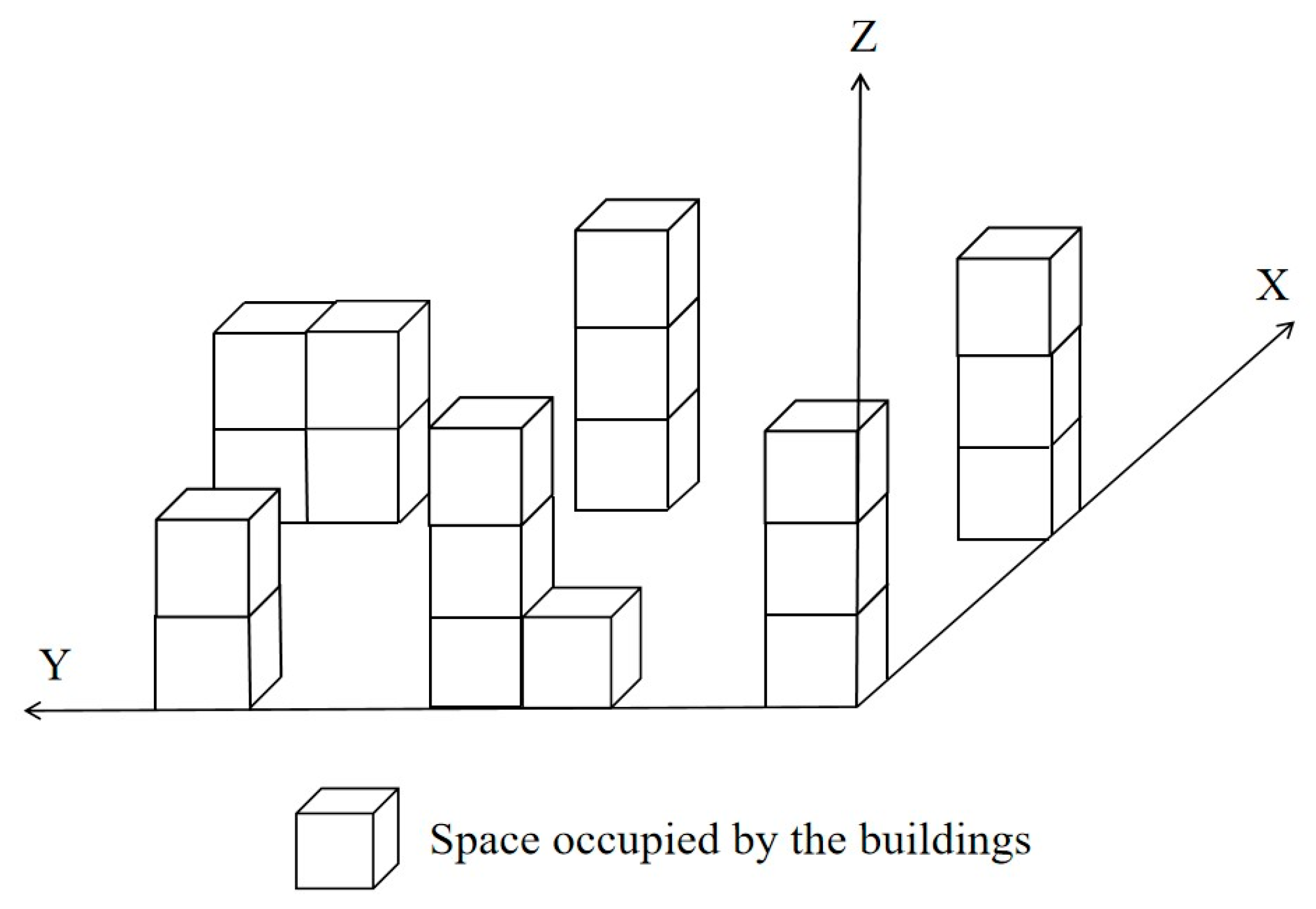
For the global planning stage, a discrete urban VLL airspace is constructed. In this paper, every static obstacle is abstracted as a rectangle, and the environment is divided into cells using a square grid with equal side lengths. Since only static obstacles are considered in the global planning stage, the flight environment is assumed to be fixed, and obstacles are known in advance.

According to the above descriptions, the VLL airspace is divided into regular grids with binary information and uses 0 and 1 to distinguish whether the grid is occupied or not, and then each grid state information can be expressed as Equation (1)

$$N_{\left(x,y,z\right)}=\left\{\begin{array}{l}0,nooccupied\\ 1,occupied\end{array}\right\},$$

(1)

where $\left(x,y,z\right)$ denotes the grid center coordinates; $N_{\left(x,y,z\right)}$ is 0 means there is no obstacle and the UAV can pass freely; $N_{\left(x,y,z\right)}$ is 1 means there is an obstacle and the UAV is forbidden to pass. The gridded airspace in the global planning stage is shown in Figure 1.

In the local trajectory planning stage, regridding will significantly increase the computational cost. Therefore, we model the airspace as a continuous space and employ trajectory planning methods for continuous space in order to generate replanning trajectories in time.

3.3. Constraints

When planning the UAV flight trajectory, the UAV’s own performance must be considered [19]; therefore, in this paper, environmental threats, obstacle threats, and multi-UAV risk distances are used as constraints to construct an objective function that considers the trajectory cost, UAV performance, etc., and the objective function is used as the trajectory evaluation index.

3.3.1. Boundary Constraint $C_1$

In the trajectory planning process, the UAV is abstracted as a mass point, and each waypoint should be guaranteed to be in the grid environment, then the boundary constraints $C_1$ can be expressed as Equation (2):

$$\left\{X_{ij}\right| X_{ij}=(x_{ij},y_{ij},z_{ij}), x_{ij}\in [0,l\cdot u], y_{ij}\in [0,l\cdot v], z_{ij}\in [0,l\cdot w], X_{ij}\in X\},$$

(2)

where $\left(x_{ij},y_{ij},z_{ij}\right)$ denotes the coordinate of the j-th waypoint of the i-th UAV; $l$ denotes the grid edge length; $u,v,w$ denote the number of grids in the $x-axis$, $y-axis$ and $z-axis$, respectively.

3.3.2. Obstacle Constraint $C_2$

In the trajectory planning process, feasible UAV trajectories cannot cross obstacles and must avoid collisions between trajectories and obstacles; therefore, the constraints of obstacles on waypoints can be expressed as follows:

$$\{X_{ij}| d\left(X_{ij},X_{i=1,2\dots ,n}^o\right)=\sqrt{{\left(x_{ij}-x_{b=1,2,\dots ,n}^o\right)}^2+{\left(y_{ij}-y_{b=1,2,\dots ,n}^o\right)}^2+{\left(z_{ij}-z_{b=1,2,\dots ,n}^o\right)}^2}>0\},$$

(3)

where $X_{ij}=(x_{ij},y_{ij},z_{ij},t_{ij}), X_{b=1,2\dots ,n}^o=(x_{b=1,2,\dots ,n}^o,y_{b=1,2,\dots ,n}^o,z_{b=1,2,\dots ,n}^o)$ and $d\left(X_{ij},X_{i=1,2\dots ,n}^o\right)$ denotes the Euclidean distance between the j-th waypoint $\left(x_{ij},y_{ij},z_{ij}\right)$ of the i-th UAV and the coordinates of all obstacles. $X_{i=1,2\dots ,n}^o$ denotes all obstacles.

3.3.3. Multi-UAV Safety Constraint $C_3$

When there are multiple UAVs in the environment, the minimum distance between UAV waypoints at the same moment should be guaranteed to be greater than the safe distance. The interpoint constraint of the UAV trajectory can be expressed as:

$$\{X_{ij}| d\left(X_{ij},X_{qk}\right)=\sqrt{{\left(x_{ij}-x_{qk}\right)}^2+{\left(y_{ij}-y_{qk}\right)}^2+{\left(z_{ij}-z_{qk}\right)}^2}+(t_{ij}-t_{qk})>0\},$$

(4)

where $d\left(X_{ij},X_{qk}\right)$ denotes distance in both time and space between the i-th UAV and the q-th UAV waypoint; $t_{ij}$ denotes the time for the i-th UAV at the j-th waypoint. $t_{qk}$ denotes the time for the q-th UAV at the k-th waypoint.

3.3.4. Target Point Constraint $C_4$

In the UAV trajectory planning problem, there is also a need for a constraint on the target point. It ensures the successful completion of the mission by requiring the existence of a planned path that starts from the initial point and ends at the specified final location. The target point constraint can be expressed as:

$$\left\{X_{ij}\right| \gamma (T)=X_{im}\},$$

(5)

where $T$ denotes the end time of trajectory $\gamma$, $\gamma (T)$ represents the position of the UAV at the end time $T$, and $X_{im}$ represents the target position of UAV-i.

3.4. Problem Modeling

In Problem 1, the path planning needs to be completed with the minimum sum of global multiple risks, while satisfying various constraints.

$$\begin{array}{l}\min \left(R_1+R_2\right)\\ s.t. C_1,C_2,C_3,C_4\end{array}\dots ,$$

(6)

where $R_1$ denotes collision risk, and $R_2$ denotes ground risk.

In Problem 2, the conflicting trajectory segment needs to be replanned to conform to the ETA of the initial flight plan, while satisfying various constraints.

$$\begin{array}{l}\min T_{diff}\\ T_{diff}=t_{real}-t_{plan}\dots .,\\ s.t. C_1,C_2,C_3,C_4\end{array}$$

(7)

where $T_{diff}$ denotes the time difference between the current time and the flight plan time, and $t_{real}$ denotes the current time, $t_{plan}$ denotes the flight plan time.

4. Review of Traditional Planning Method

4.1. Standard A*

The A* algorithm is a heuristic graph search algorithm, which is based on the Dijkstra heuristic search algorithm [20], and the search framework is the same as Dijkstra’s algorithm, but the A* algorithm heuristic function is better than Dijkstra’s algorithm for fast search of the shortest trajectory. According to [21], the heuristic function of the A* algorithm is Equation (8):

$$\begin{array}{cc}\hfill f\left(n\right)& =g\left(n\right)+h\left(n\right)\hfill \\ & =\left|X_n-X_0\right|+\sqrt{{\left(X_n-X_m\right)}^2}\end{array},$$

(8)

where $n$ denotes the current node; typically, $g\left(n\right)$ denotes the accumulation cost, calculated using the Manhattan distance; $h\left(n\right)$ denotes the target cost, applying the Euclidean distance as a function estimate;$X_n$ is the current point; $X_0$ is the starting point;$X_m$ is the target point.

4.2. Standard PSO

The particle swarm algorithm is a population intelligence optimization algorithm proposed by Kennedy and Eberhart [22] in 1995, and its most important advantage is that the algorithm can be achieved by controlling several parameters. When applied to trajectory planning [23], the best fitness in each iteration is shown in Equation (9):

$$\left\{\begin{array}{l}{X}_{ijb}^k=\left\{X_{i1}^1,X_{i2}^2,X_{i3}^3,\cdots ,X_{ij}^k\right\}\\ X_g^k=\left\{X_1^k,X_2^k,X_3^k,\cdots ,X_j^k\right\}\end{array}\right.,$$

(9)

where $X_{ijb}^k$ is the j-th local optimal particle position of UAV-i in the k-th generation; $X_g^k$ is the j-th global optimal particle position in the k-th generation.

In the iterative process, the local optimal individual and the global optimal individual in each generation are obtained, and the next velocity and position of the particle are determined according to the update formula. The traditional particle swarm algorithm velocity and position update formula is shown in Equation (10):

$$\left\{\begin{array}{l}{V}_{ij}^{k+1}=\omega V_{ij}^k+c_1{\xi }_1\left(X_{ijb}^k-X_{ij}^k\right)+c_2{\xi }_2\left(X_g^k-X_{ij}^k\right)\\ X_{ij}^{k+1}=X_{ij}^k+V_{ij}^{k+1}\end{array}\right.,$$

(10)

where $\omega$ is the inertia weighting factor, the larger $\omega$ the easier it is for the particle to explore the unknown trajectory; $c_1$ is the individual learning factor, which indicates the influence weight of the local optimal particle; $c_2$ is the population learning factor, which indicates the influence weight of the global optimal particle; ${\xi }_1$ and ${\xi }_2$ are two random numbers between (0,1) to increase the exploration range of the particles during the search; the particle velocity range is$\left[-v_{\max },v_{\max }\right]$.

5. Method

5.1. Two-Stage Air Logistics Transportation Trajectory Planning Method

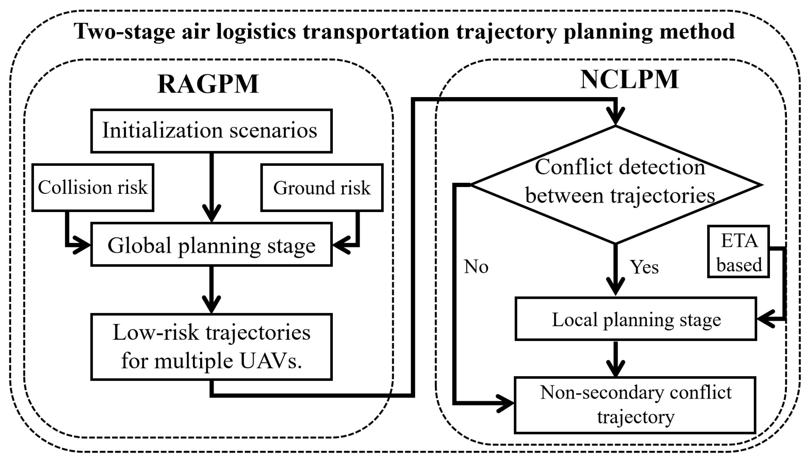
This study presents a dual-phase trajectory planning framework for high-density logistics UAV operations, comprising: (1) a risk-aware global planning module (RAGPM) incorporating collision risk assessment and ground hazard evaluation; (2) a non-secondary conflict local planning module (NCLPM) that dynamically replans trajectories while preventing secondary conflicts through ETA-based optimization. The overall algorithm flow is shown in Figure 2.

5.2. Risk Aware Global Planning Module (RAGPM)

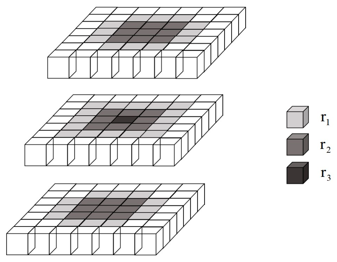
When applying the A* algorithm to multi-UAV global trajectory planning, traditional methods do not consider the ground risk. Therefore, our approach takes into account both collision risk and ground risk. Firstly, we will introduce the collision risk. To obtain a globally safe initial trajectory, this paper takes the obstacles as the center, fully considers the collision risk between the aircraft and the obstacles, and divides the environment into three risk levels according to the distance from the nearest obstacle grid. The closer the grid is to the obstacle, the higher the risk level; conversely, the lower the risk level, as shown in Equations (11)–(13):

$$\begin{array}{c}{R}_1\left(X_{ij},X_{b=1,2\dots ,n}^o\right)={\max }_{b=0}^n\left\{R_1\left(X_{ij},X_b^o\right)\right\}\end{array},$$

(11)

$$risk\left(X_{ij},X_{b=1,2\dots ,n}^o\right)=\left\{\begin{array}{l}{r}_1,0<d\left(X_{ij},X_{b=1,2\dots ,n}^o\right)\le \sqrt{3}\\ r_2,\sqrt{3}<d\left(X_{ij},X_{b=1,2\dots ,n}^o\right)<3\\ r_3,d\left(X_{ij},X_{b=1,2\dots ,n}^o\right)\ge 3\end{array}\right.,$$

(12)

$$d\left(X_{ij},X_{b=1,2\dots ,n}^o\right)={\min }_{b=0}^k\left\{\sqrt{{\left(X_{ij}-X_b^o\right)}^2}\right\},$$

(13)

where $R_1\left(X_{ij},X_{b=1,2\dots ,n}^o\right)$ is the grid$\left(x_i,y_i,z_i\right)$ risk level; $b$ is the number of obstacles; $risk\left(X_{ij},X_{b=1,2\dots ,n}^o\right)$ is the grid risk level criterion; $d\left(X_{ij},X_{b=1,2\dots ,n}^o\right)$ is the Euclidean distance between $X_{ij}$ and the center of the obstacle $X_{b=1,2\dots ,n}^o$. The risk level classification diagram is shown in Figure 3, the gradation from dark to light corresponds to the transition from higher risk $r_3$ to lower risk $r_1$.

According to the security requirements, it is specified that the cost is higher when expanding from low-risk grid to high-risk grid. In practice, without compromising generality, we set $r_1=1$, $r_2=4$ and $r_3=9$.

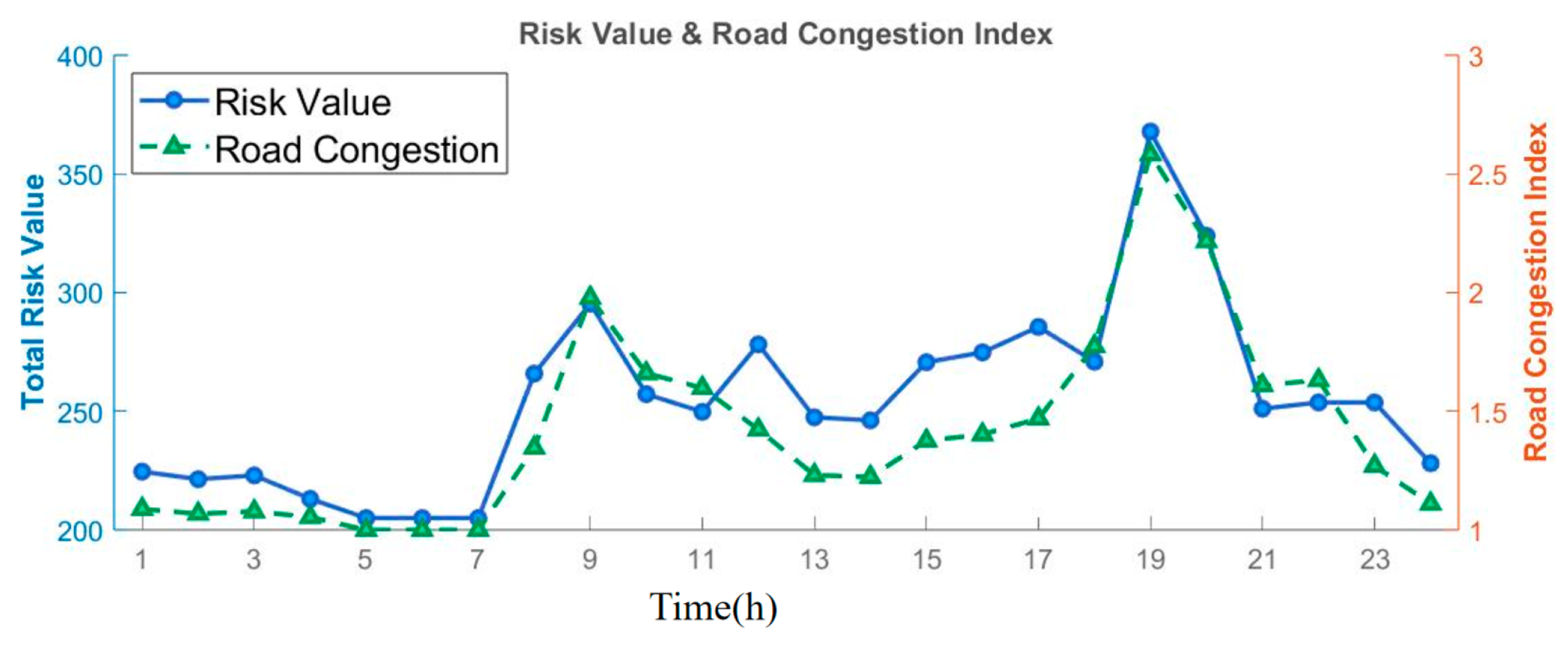
In terms of ground risk, according to reference [24], quantifying the intrinsic risk posed by potential UAV crashes to ground populations is a preferred method of analysis, and the quantified ground risk can be formed into a risk map [25] in the form of a grid for subsequent trajectory planning calculations. The fatality rate of UAV collisions with pedestrians, defined as the number of deaths resulting from such incidents over a certain period of time, is selected as the indicator for assessing ground risk. When calculating risk, it is also necessary to consider the volatility during peak hours or special times. According to data from Baidu Map’s traffic and travel big data platform, urban traffic flow exhibits significant periodic patterns. In conjunction with the research in references [26,27], the risk values of urban population density also demonstrate periodic characteristics. Therefore, the road congestion index during the current time period will be incorporated when considering risk values. According to references [28,29], ground risk is primarily related to population density, and the calculation method for ground risk is as follows:

$$R_2(n)=CI·A\lambda F(n){\rho }_P(n),$$

(14)

where $A$ denotes the area of the ground hit by the UAV within the grid, $\lambda$ denotes the probability of such an accident occurring per unit of flight time, $F$ denotes the lethal probability upon hitting a person, ${\rho }_P$ denotes population density. $CI$ denotes congestion index.

According to reference [30], the lethal probability of hitting personnel is mainly derived from the dynamic analysis of UAV.

$$\begin{array}{c}F={\displaystyle \frac{1}{1+\sqrt{\frac{\mathrm{b}}{d}}{\left(\frac{d}{E_{imp}}\right)}^{\frac{1}{4c_s}}}}\\ E_{imp}={\displaystyle \frac{1}{2}}m{v}^2,v=\sqrt{{\displaystyle \frac{2h}{g}}}\end{array},$$

(15)

The lethal probability upon hitting a person is obtained through UAV dynamic analysis, through the force analysis of kinetic energy and gravitational potential energy, the speed of the UAV can be converted into $v=\sqrt{\frac{2\mathrm{h}}{g}}$. Substitute $v$ into $E_{imp}$, integrate and simplify the parameters in $F$. A simplified formula can be obtained as shown in the following Equation (16):

$$F={\displaystyle \frac{\alpha m^{2}gh}{\beta }},$$

(16)

where $\alpha$ denotes hyperparameters related to the UAV model, and $\beta$ denotes hyperparameters related to the impact energy, $h$ denotes the flight altitude of the UAV.

By incorporating the risk level cost function values into the heuristic function $f\left(n\right)$, the RAGPM heuristic function $W\left(n\right)$ is shown in Equation (17):

$$W\left(n\right)=f\left(n\right)+R_1\left(n\right)+R_2\left(n\right),$$

(17)

where $W\left(n\right)$ denotes the estimated cost function, based on Equation (6); $r\left(n\right)$ denotes the risk level cost function.

5.3. Non-Secondary Conflict Local Planning Module (NCLPM)

After completing the global planning stage, it is necessary to replan for UAVs whose trajectories conflict with each other. To avoid secondary conflicts in the replanned trajectories, this paper proposes the NCLPM to address this issue. This module has been improved by integrating the PSO algorithm and the APF method and incorporates ETA to prevent the occurrence of secondary conflicts.

5.3.1. Spatial and Temporal Conflict Detection

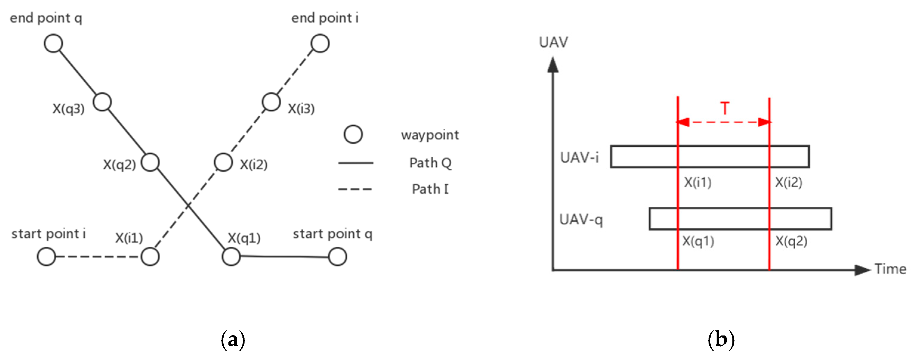
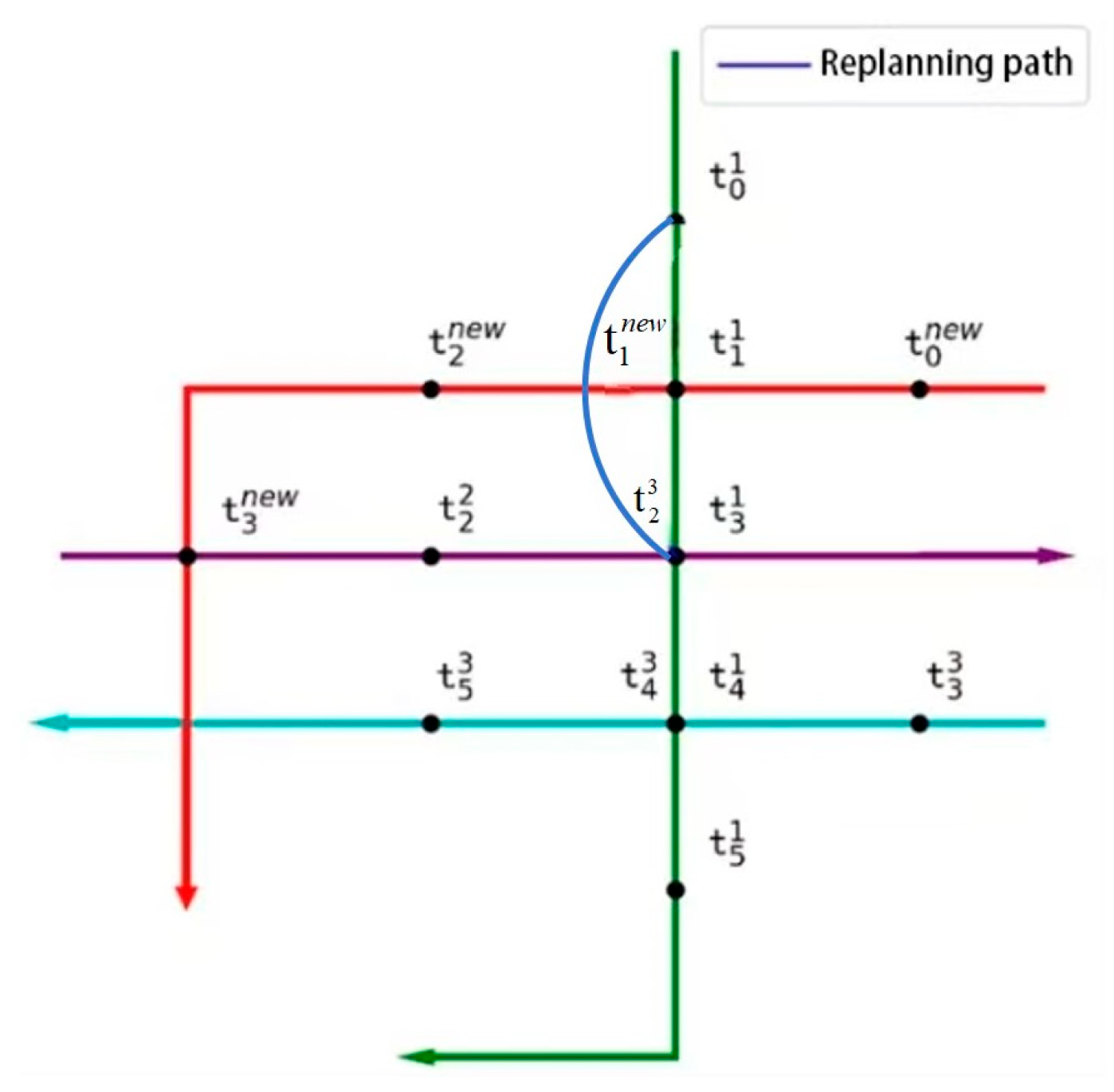
Traditional conflict detection primarily focuses on conflicts in the spatial dimension. However, in high-density operational scenarios, the temporal dimension also needs to be considered. Therefore, we propose a simple method for spatial and temporal conflict detection. For spatial conflict detection, assuming the spatial diagram of UAV-i and UAV-q is as shown in Figure 4a, the method will compare the distance between each waypoint of UAV-i and UAV-q. For temporal conflict detection, assuming the temporal diagram of UAV-i and UAV-q is as shown in Figure 4b, for waypoints where spatial conflicts occur, the time difference between the two UAVs arriving at that waypoint is checked. If the time difference is less than the allowed safe time, it is considered that UAV-q and UAV-i will collide in that segment of spatial and temporal trajectory.

5.3.2. Fitness Function Based on ETA

ETA prediction is crucial in various applications. In the transportation sector, ETA is used to predict the arrival times of ships [31] and flights [32], as well as for traffic congestion forecasting [33]. In the military field, it aids in coordinating attack operations [34]. Through ETA prediction, the time for drones to arrive at specified waypoints from different locations can be estimated.

Upon detecting a conflict, following the first-come-first-served principle, we are only replanning the lower-priority UAV of the conflict. However, when the existing 4D trajectory planning algorithm carries out conflict replanning, it does not consider the initial flight plan, so the trajectory after replanning is different from the initial flight plan, and the arrival time of the next waypoint changes, which may lead to the secondary conflict between the subsequent trajectory and other trajectories. Therefore, to avoid secondary conflicts between the replanning trajectory and the remaining trajectories after local replanning, this paper introduces ETA prediction as a goal to minimize the impact on the initial flight plan.

In a fitness function based on ETA, each particle consists of the waypoint coordinates and the current point flight time, thus adapting to the multi-UAV 4D collaborative trajectory replanning problem. The state space of the p-th particle of UAV-i in the k-th generation can be expressed as (18):

$$\begin{array}{cc}\hfill X_{ip}^k& =\left(x_{ip}^k,y_{ip}^k.z_{ip}^k,t_{ip}^k\right)\hfill \\ \hfill t_{ip}^k& ={\displaystyle \frac{{\displaystyle \sum _{k=0}^{k-1}\sqrt{{\left(X_{ip}^k-X_{ip}^{k+1}\right)}^2}}}{v_i}}\hfill \end{array},$$

(18)

where $v_i$ denotes the flight speed of UAV-i; $t_{ip}^k$ denotes the time for particle p to fly from the starting point to the current point with speed $v_i$; k denotes the number of iterations of the particle swarm algorithm, and when k = 0 denotes the initial position of the UAV, set as Equation (19):

$$\begin{array}{cc}{X}_{ip}^0=\left(x_{is}+\phi ,y_{is}+\phi ,z_{is}+\phi ,0\right)& \phi \in [-0.5,0.5]\end{array},$$

(19)

where $\phi$ is a random number.

Fitness of the particles. When particles are searching for a trajectory, in order to replan the trajectory without interfering with the original initial flight plan, the flight time to the next waypoint is used as the fitness function of the PSO algorithm, and the fitness of the particles is better the closer it is to the originally scheduled arrival time. The fitness function is shown in Equation (20):

$$\begin{array}{cc}\hfill fi{t}_{ib}^k& =\min \left\{ET{A}_p-\left(t_{ip}^k+Et{h}_{ip}^k\pm \Delta \right)\right\}\hfill \\ \hfill ET{A}_{i,j}& ={\displaystyle \frac{{\displaystyle \sum _{j=j-1}^j\sqrt{{\left(X_{ij}-X_{i,j+1}\right)}^2}}}{v_i}}\hfill \\ \hfill Et{h}_{ip}^k& ={\displaystyle \frac{\sqrt{{\left(X_{ip}^k-X_{ig}\right)}^2}}{v_i}}\hfill \end{array},$$

(20)

where $fi{t}_{ib}^k$ denotes the optimal fitness in the k-th iteration; $ET{A}_{i,j}$ denotes the flight time of the original conflicting trajectory part; $Et{h}_{ip}^k$ denotes the time of flight from the current coordinate $X_{ip}^k$ of the p-th particle of UAV-i in the k-th iteration to the target point $X_{ig}$ Euclidean distance;$\Delta$ indicates the arrival time margin.

5.3.3. Location Update Formula Based on APF

For the two-stage air logistics transportation trajectory planning problem, the traditional PSO has the following defect: low convergence accuracy. In contrast, the APF method [35], proposed by Oussama Khatib in 1985, guides robots to perform safe and smooth trajectory planning in their environment by simulating the interaction of at-tractive and repulsive forces, having the advantage of simply computing and real-time calculating. However, the problem of local optimum [36] and unreachability of the target point usually occurs [37].

Therefore, the NCLPM proposed in this paper fully considers the advantages of both PSO and APF algorithms and combines the two to propose an improved PSO based on APF. Specifically, additional repulsion between UAVs, global optimal particle guidance force, and improved repulsion force are incorporated into the algorithm as additional forces.

Additional repulsion between UAVs. In the process of NCLPM, this paper prevents collisions between UAVs by attaching inter-UAV repulsions. During the searching progress, the additional repulsive force on the UAV is added when the Euclidean distance between $X_{ip}^k$ and $X_{qj}$ is smaller than the safe distance and defined as Equation (21):

$$\begin{array}{cc}\hfill F_{rep\_U}\left(X_{ip}^k\right)& =-\nabla U_{rep\_U}\left(X_{ip}^k\right)\hfill \\ & =\left\{\begin{array}{cc}-k_{rep}\left({\displaystyle \frac{1}{\rho \left(X_{ip}^k,X_{qj}\right)}}-{\displaystyle \frac{1}{r}}\right){\displaystyle \frac{1}{{\rho }^2\left(X_{ip}^k,X_{qj}\right)}}& ,\rho \left(X_{ip}^k,X_{qj}\right)\le r\\ 0& ,\rho \left(X_{ip}^k,X_{qj}\right)>r\end{array}\right.\end{array},$$

(21)

where $r$ is the repulsive range of action; $\rho \left(X_{ip}^k,X_{qj}\right)$ denotes the Euclidean distance between $X_{ip}^k$ and $X_{qj}$.

Global optimal particle guidance force. To address the local optimum problem, this paper reduces the probability of the algorithm falling into a local optimum by introducing additional global heuristic guidance. In the k-th iteration, the particle with the best fitness function value from Equation (20) is selected as the global optimal particle, and its attraction to the other particles is increased, thereby improving search efficiency while reducing the probability of the algorithm falling into a local optimum. The guidance force exerted by the global optimal particle on the other particles is represented by Equation (22):

$$F_{att2}\left(X_{ip}^k\right)=-k_{ib}\rho \left(X_{ip}^k,X_{ib}^k\right){\displaystyle \frac{\partial \rho \left(X_{ip}^k,X_{ib}^k\right)}{\partial \left(X_{ip}^k\right)}},$$

(22)

where $k_{ib}$ is the gravitational gain coefficient of the globally optimal particle; $X_{ib}^k$ is the coordinates of the particle with optimal fitness in the k-th iteration; $\rho \left(X_{ip}^k,X_{ib}^k\right)$ denotes the Euclidean distance from the current position of the p-th particle of UAV-i to the global optimal particle in the k-th iteration.

Improved repulsion force. According to APF, when there are obstacles near the target point, as the UAV gradually approaches the target point, the gravitational force from the target point will continue to decrease, while the repulsive force from the obstacles will continue to increase, leading to the problem of being unable to reach the target point due to insufficient gravitational force. To address this issue, this paper refers to the literature [38] and adopts an improved repulsive potential field method to prevent the UAV from being unable to reach the target point due to insufficient gravitational force in the vicinity of the target point.

The repulsive force on the particle is obtained in the direction of the decreasing gradient is shown in Equation (23):

$$F_{rep}^{\prime }\left(X_{ip}^k\right)=-\nabla U_{rep}^{\prime }\left(X_{ip}^k\right)=\left\{\begin{array}{l}{F}_{rep1}+F_{rep2},\rho \left(X_{ip}^k,X_O\right)\le r\\ 0,\rho \left(X_{ip}^k,X_O\right)>r\end{array}\right.,$$

(23)

where $F_{rep1}$ and $F_{rep2}$ are defined as follows:

$$\begin{array}{cc}\hfill F_{rep1}& =k_{rep}\left({\displaystyle \frac{1}{\rho \left(X_{ip}^k,X_O\right)}}-{\displaystyle \frac{1}{r}}\right){\displaystyle \frac{{\rho }^n\left(X_{ip}^k,X_{ig}\right)}{{\rho }^2\left(X_{ip}^k,X_O\right)}}{\displaystyle \frac{\partial \rho \left(X_{ip}^k,X_o\right)}{\partial \left(X_{ip}^k\right)}}\hfill \\ \hfill F_{rep2}& =-{\displaystyle \frac{n}{2}}{k}_{rep}{\left({\displaystyle \frac{1}{\rho \left(X_{ip}^k,X_O\right)}}-{\displaystyle \frac{1}{r}}\right)}^2{\rho }^{n-1}\left(X_{ip}^k,X_{ig}\right){\displaystyle \frac{\partial \rho \left(X_{ip}^k,X_{ig}\right)}{\partial \left(X_{ip}^k\right)}}\hfill \end{array},$$

(24)

and $\rho \left(X_{ip}^k,X_O\right)$ denotes the Euclidean distance from the current position of the p-th particle of UAV-i to the center of the obstacle in the k-th iteration; $\rho \left(X_{ip}^k,X_{ig}\right)$ denotes the Euclidean distance from the current position of the p-th particle of UAV-i in the k-th iteration to the target point $X_{ig}$. As can be seen from the formula, as the UAV continues to move toward the target point, the gradual increase can avoid the situation where the combined force is 0, making the UAV continue to move toward the target point, thus solving the problem of unreachability of the target point.

Position update formula. When using NCLPM for trajectory search, the resultant force on the particles is composed of Equations (21)–(23). Then, the resultant force on the p-th particle of UAV-i in the k-th iteration is shown in Equation (25):

$$\begin{array}{cc}\hfill F\left(X_{ip}^k\right)& =F_{att}+F_{rep}\hfill \\ & =F_{att}\left(X_{ip}^k\right)+F_{att2}\left(X_{ip}^k\right)+{\displaystyle \sum _{\mathrm{q}=0}^u{F}_{rep\_U}\left(X_{ipq}^k\right)}+{\displaystyle \sum _{o=0}^n{F}_{rep}^{\prime }\left(X_{ipo}^k\right)}\hfill \end{array},$$

(25)

where $u$ is the number of UAVs; $n$ is the number of obstacles.

Based on the PSO algorithm, assume that the velocity of the p-th particle of UAV-i at the k-th iteration is $V_{ip}^k$, when k = 0 the initial velocity of the UAV is $V_{ip}^0\in \left[0,1\right]$, limiting the particle velocity in the range of$\left[-v_{\max },v_{\max }\right]$. In the iterative process, since a particle represents a waypoint, only the effect of the global optimal particle position feature on the particle velocity update is considered, and the velocity varies randomly in a certain range with the number of iterations, the velocity update equation can be expressed as (26):

$$\begin{array}{c}{V}_{ip}^{k+1}=\omega V_{ip}^k+c_2{\xi }_2\left(X_{ib}^k-X_{ip}^k\right)\\ V_{ip}^{k+1}=\left\{\begin{array}{l}{v}_{\max },V_{ip}^{k+1}>v_{\max }\\ -v_{\max },V_{ip}^{k+1}<-v_{\max }\end{array}\right.\end{array},$$

(26)

where$X_{ib}^k$ denotes the optimal position of each particle.

In summary, in NCLPM, the update of particle position is guided by the improved APF together with the PSO algorithm; thus, the update formula of particle position is shown in Equation (27):

$$X_{ip}^{k+1}=X_{ip}^k+V_{ip}^{k+1}+l\cdot {\displaystyle \frac{F\left(X_{ip}^k\right)}{‖F\left(X_{ip}^k\right)‖}},$$

(27)

where $l$ is the search step of the APF method.

5.4. Pseudo Code of Two-Stage Air Logistics Transportation Trajectory Planning Algorithm

The pseudo code of the two-stage air logistics transportation trajectory planning algorithm is shown in Algorithm 1, and the specific steps are as follows:

In lines 2–4 of Algorithm 1, the algorithm first initializes the necessary parameters and sets the starting point for the UAV’s flight plan, as well as generates the map and risk map required for trajectory planning and collects information about the obstacles present in the map to generate an obstacle list.

In lines 5–8 of Algorithm 1, for each UAV, RAGPM is used for global trajectory planning to generate a trajectory from the starting point to the target point. And based on RAGPM, the flight plan is set in lines 9–10.

In lines 11–17 of Algorithm 1, conflict detection is performed to check if there are any conflicts between the UAV flight plans. If a conflict is detected, the algorithm initiates the conflict resolution process. If a conflict occurs, the algorithm first determines the specific location of the conflict and obtains the starting and ending points for the replanned trajectory. Then, NCLPM is used to generate a new trajectory between the conflict points, and the flight plan is updated based on this new trajectory. Finally, the algorithm returns the updated flight plan. In lines 17, the flight plan output by this algorithm consists of four-dimensional trajectory points, which aligns with the interface requirements of NASA’s open-source API for UAM [39].

Algorithm 1 Two-stage air logistics transportation trajectory planning algorithm
1	procedure planning
2	Initialize parameters
3	Generate map and risk map: GenerateMap(map)
4	Collect obstacles: obstacle list ← CollectObstacles(map)
5	Generate paths using RAGPM:
6	for i = 0 to l do
7	path_i ← RAGPM (map, start_points1, target_points1, risk_map)
8	end for
9	Calculate flight plans:
10	flight_plans ← CalculateFlightPlans (path, UAV_speed)
11	Detect conflicts:
12	if ConflictsDetected(flight_plans) then
13	start_pos2, target_pos2 ← DetermineConflictPoints(flight_plans)
14	replanning_path ← NCLPM (start_pos2, target_pos2, obstacle list, flight_plans)
15	Update flight_plans with replanning_path
16	end if
17	Return flight_plans
18	end procedure

6. Simulation and Results

To demonstrate the effectiveness of the proposed two-stage air logistics transportation trajectory planning algorithm in the VLL urban logistics scenario, five simulation experiments are set up.

All experiments were conducted in a MATLAB^® 2019b programming environment using an Intel Core i5-12600KF CPU @ 3.60GHz 10-core with 32G of running memory. Since different parameters in NCLPM have different effects on the UAV trajectory planning, the algorithm in this paper involves the relevant parameters.

For the parameters involved, $p$ is the number of particles in the particle swarm, with a value of 50; $\omega$ is the inertia weighting factor, set at 1.2; $v_{\max }$ is the maximum particle velocity, which is 1; $k_{att}$ is the gravitational gain coefficient, valued at 15; $k_{rep}$ is the repulsion gain coefficient, with a value of 25; $max\_iters$ is the iteration number, set to 800; $c_2$ is the population learning factor, with a value of 2; $l$ is the step length, which is 0.05; $r$ is the safe distance between UAVs and the repulsive range of action, set at 2; $k_{ib}$ is the gravitational gain coefficient of the globally optimal particle, with a value of 0.3.

6.1. Overall Performance of Two-Stage Air Logistics Transportation Trajectory Planning Algorithm

To assess the overall performance of the proposed two-stage air logistics transportation trajectory planning algorithm, a simulation scenario based on urban VLL logistics is constructed. This scenario serves as a platform for comparing the algorithm against two benchmarks: the conflict-free A* algorithm (CFA*) in AirMatrix [13] and the traditional A* algorithm, all operating within the same context.

Set the map size of the urban VLL logistics simulation scenario to 600 m × 600 m × 60 m; the grid size is taken as 10 m. This experiment extracts the population density of a certain area in Chengdu, Sichuan Province, China, as the population density for the current map and calculates based on the average road congestion index from March 14, 2025, in Chengdu, using data sourced from Baidu Map’s Transportation and Travel Big Data Platform [40]. The risk values corresponding to the road congestion index are shown in Figure 5. The reason why the risk value is not directly proportional to the road congestion index is that the road congestion index causes the risk value to constantly change, leading to the re-planning of the trajectory in the global phase as the risk value varies, rather than consistently following the same trajectory.

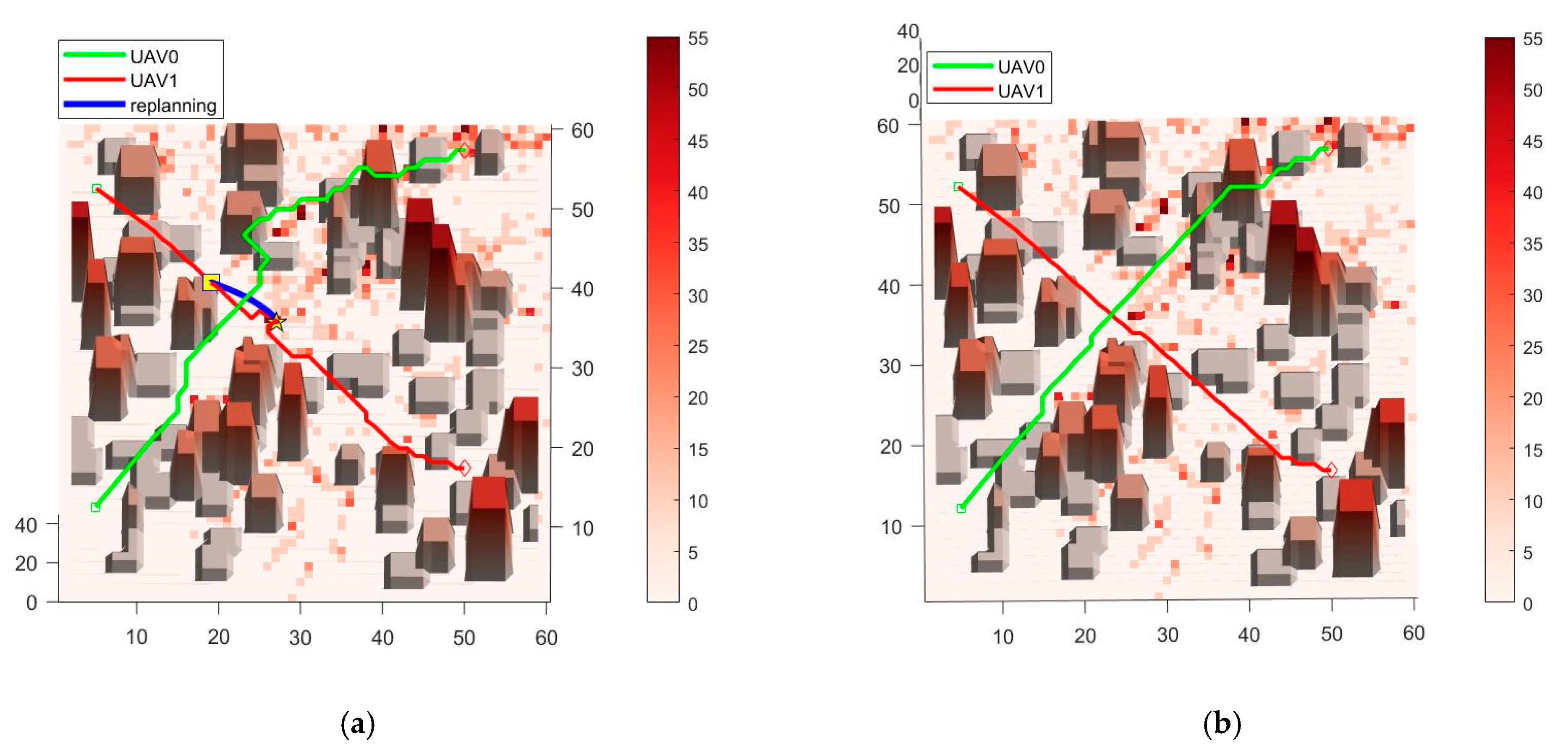
After conducting 100 experiments, the common result of the algorithm in this paper and the conflict-free A* algorithm in AirMatrix trajectory planning is shown in Figure 6, and the comparison of evaluation metrics is shown in

Table 1. Evaluation indicators for overall performance.

Method	Risk Value	Trajectory Distance(m)	Planning Time (s)	Average Delay(s)	Collision
Proposed	14.00	71.0727	2.4906	1.5896 × 10−3	No
CFA*	73.00	67.9253	0.3877	7.9260	No
A*	73.00	67.9253	0.3608	None	Yes

. When using RAGPM directly, UAV-0 and UAV-1 will have a conflict at the point (20,35,20). Therefore, according to the algorithm process, local replanning NCLPM will be performed on UAV-1, which has a lower priority at this time. The waypoint (20,35,20) is set as the replanning start point represented as a yellow square in Figure 6a, and the next conflict-free waypoint (26,31,22) is set as the replanning target point, represented as a yellow star in Figure 6a.

Using NCLPM, a replanned trajectory can be obtained, as shown by the blue trajectory in Figure 6a, which illustrates the replanning schematic. In contrast to the local replanning performed by NCLPM, the conflict-free A* algorithm resolves conflicts by instructing the UAV to hover in place and wait, as depicted in Figure 6b. Although this approach resolves the immediate conflict, it compromises the real-time performance that UAVs should possess in urban logistics transportation and poses the risk of secondary conflicts arising.

The spatial trajectories generated by the traditional A* algorithm and the CFA* algorithm are identical, so only the diagram of the CFA* algorithm is shown. As can be seen from Figure 6, the trajectories planned by both the traditional A algorithm and the CFA* algorithm have lower costs, but they are near obstacles and do not consider the ground risk related to population density, failing to avoid areas with higher population density on the map, which can lead to high-risk operation. As shown in Figure 7, the diagram illustrates the optimization process of the local stage algorithm. The yellow square represents the starting point, and the yellow star represents the endpoint.

Table 1 encompasses the evaluation metrics of the two-stage air logistics transportation trajectory planning algorithm, the CFA* algorithm, and the conventional A* algorithm. Specifically, it includes risk value, trajectory distance, planning time, the average delay time, and whether conflicts occur. The risk value is defined as the sum of collision risk and ground risk values across the entire trajectory. From Table 1, it can be observed that the two-stage air logistics transportation trajectory planning algorithm proposed in this paper reduces the risk value by 80.82% compared to both the CFA* algorithm and the traditional A* algorithm. However, compared to the CFA* and A* algorithms, this algorithm increases some additional planning time. Nevertheless, considering the substantial improvement in safety, the increased planning time is deemed acceptable. Additionally, the CFA* algorithm exhibits a delay in arrival time, while the A* algorithm results in conflicts between two UAVs.

After simulation and comparative experiments, the results indicate that the method proposed in this paper can achieve the goal of replanning without secondary conflicts while preserving the global initial flight plan. Moreover, compared to the CFA* and A* algorithms, it can effectively reduce collision risk and ground risk with only a slight increase in trajectory distance and planning time.

6.2. Case Study of Low-Risk Global Planning

This case will compare the effectiveness of RAGPM and traditional CFA* algorithms in global planning capabilities. The scenario is still set to an urban VLL scenario, with a map size of 100 m × 100 m × 100 m and a grid size of 10 m. The starting point and end point of the two UAVs are the same. As shown in

Table 2. Evaluation indicators for global planning stage.

Method	Trajectory Distance(m)	Collision Risk	Ground Risk	Overall Risk
RAGPM	19.8995	60.00	37.00	97.00
CFA*	14.4853	97.00	106.00	203.00

, the evaluation will be based on the following indicators: the trajectory distance, the risk value of collision risk, the risk value of ground risk, and the risk value of overall risk.

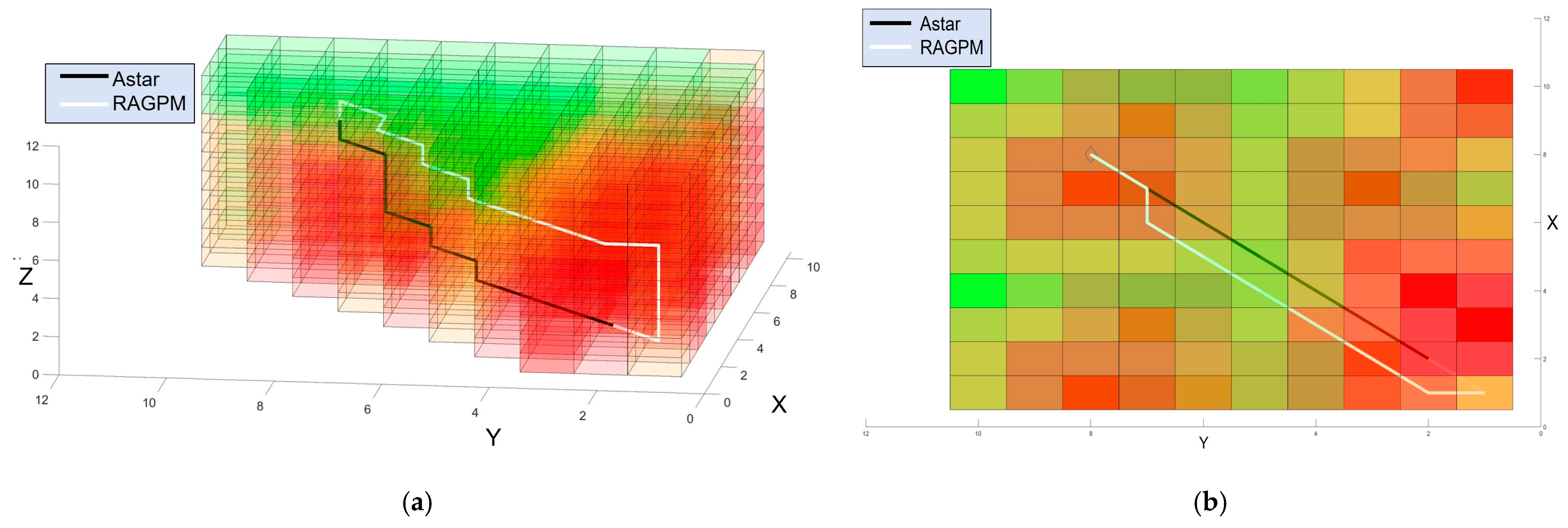
As can be seen from Table 2, the two trajectory planning methods, RAGPM and CFA*, exhibit significant differences in trajectory distance, collision risk, ground risk, and overall risk. Although the CFA* method performs slightly better in trajectory distance, with a reduction of approximately 27.3% compared to RAGPM, RAGPM demonstrates lower risk levels in collision risk, ground risk, and overall risk, with reductions of approximately 38.1%, 65.1%, and 52.2% compared to the CFA* method, respectively. Figure 8 showcases the trajectories planned by RAGPM and A* in a risk grid under visualization conditions.

6.3. Case Study of Non-Secondary Conflict Local Replanning

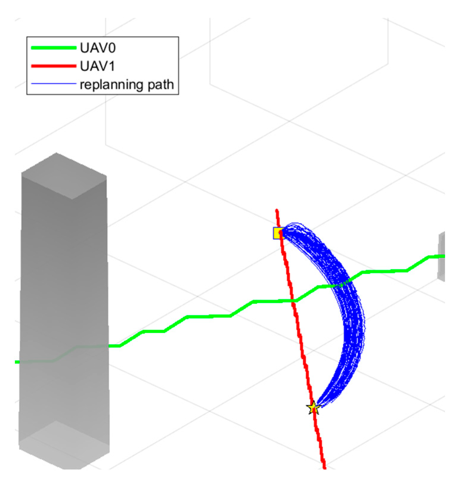
We use the same environment as Section 6.1, and for the replanning case, the point (20,35,20) is set as the replanning starting point, and the point (26,31,22) is set as the replanning target point. The results of the proposed algorithm in local replanning are shown in Figure 9. In Figure 9, the yellow square represents the starting point, and the yellow star represents the endpoint.

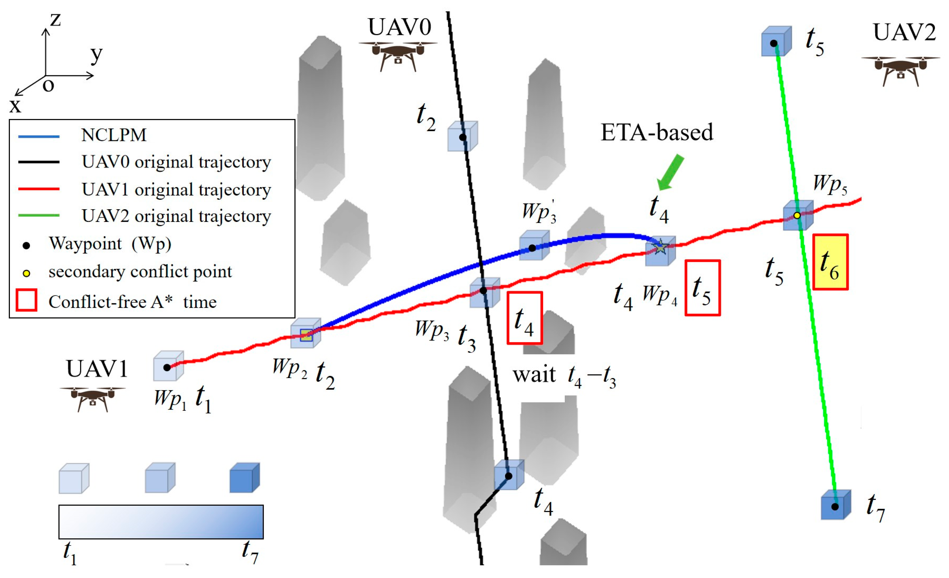
As evident from the simulation result depicted in Figure 9, the trajectory planned by NCLPM significantly deviates from that of CFA*. When conflicts arise between two UAVs in both spatial and temporal dimensions, the waypoints immediately preceding the local replanning and NCLPM are used to replan the conflicting trajectory. The blue line in the figure represents the replanned trajectory, which clearly exhibits a replanning solution for the local conflict. In Figure 9, a conflict occurs between UAV-0 and UAV-1 from UAV-1′s waypoint 2 to waypoint 4. If the CFA* method is adopted, where the conflicting UAV is made to wait, it will arrive at waypoint 4 at time $t_5$ and subsequently create a secondary conflict with UAV-2, which also arrives at waypoint 5 at time $t_6$. In contrast, after re-planning based on ETA using the NCLPM, UAV-1 will arrive at waypoint 4 at time $t_4$, in line with the original flight plan, and will not conflict with UAV-2 afterwards, significantly reducing the likelihood of subsequent trajectory conflicts with other UAVs.

In

Table 3. Evaluation indicators for local replanning stage.

Method	UAV Flight Density	Secondary Conflict	Delay Time
NCLPM	3	No	0.0075
	6	No	0.0942
	9	No	0.1012
CFA*	3	No	7.9486
	6	Yes	27.7743
	9	Yes	42.6395

, UAVs of different flight densities were tested under the same scenario, and the corresponding delay times as well as whether secondary collisions occurred were recorded. Based on the results, as the flight density increases, both methods experience increased delay times. However, CFA* exhibits significantly more delay, while the delays for NCLPM remain roughly constant. Furthermore, as the delay time increases, CFA* can lead to secondary collisions. Meanwhile, the delay time of NCLPM is also reduced by 99.66–99.9% compared to CFA*.

Through simulation experiments, it can be found that both the CFA* algorithm and the NCLPM algorithm can avoid conflict points when conflicts occur between UAVs. On this basis, the NCLPM algorithm can not only guide the replanned UAV to reach the designated point within the specified time but also avoid the secondary conflicts that may arise from CFA*, thereby effectively improving the safety of the replanned trajectory.

6.4. Application Case of Large-Scale Urban Scenarios

To demonstrate the method proposed in this paper can be directly applied in real-world scenarios, a large-scale urban scenario was established for this simulation. Specifically, this scenario features a map size of 3000 m × 3000 m × 120 m, a grid edge length of 10 m, and an obstacle ratio of 8%. Furthermore, at the strategic trajectory planning level, 11 UAV flight plans provided by operators are set, with the starting and ending coordinates as well as the takeoff time of UAV0-UAV10 presented in

Table 4. UAV flight plans.

UAV	Start Point	End Point	Take-Off Time
UAV-0	(147,168,0)	(93,60,0)	11:03
UAV-1	(51,120,0)	(150,30, 0)	10:54
UAV-2	(177,150,0)	(138,153,0)	8:12
UAV-3	(162,87,5)	(144,165,0)	10:44
UAV-4	(78,108,0)	(84,111,0)	11: 04
UAV-5	(18,6,0)	(129,57,0)	10:07
UAV-6	(144,27,0)	(168,153,5)	9:06
UAV-7	(105,87,0)	(48,102,0)	9:21
UAV-8	(126,18,0)	(69,117,0)	9:54
UAV-9	(132,90,0)	(126,87,0)	10: 26
UAV-10	(18,144,0)	(123,57,0)	9:38

. Due to wind speed and weather conditions, the flight plan of UAV-10 was delayed, leading to a conflict.

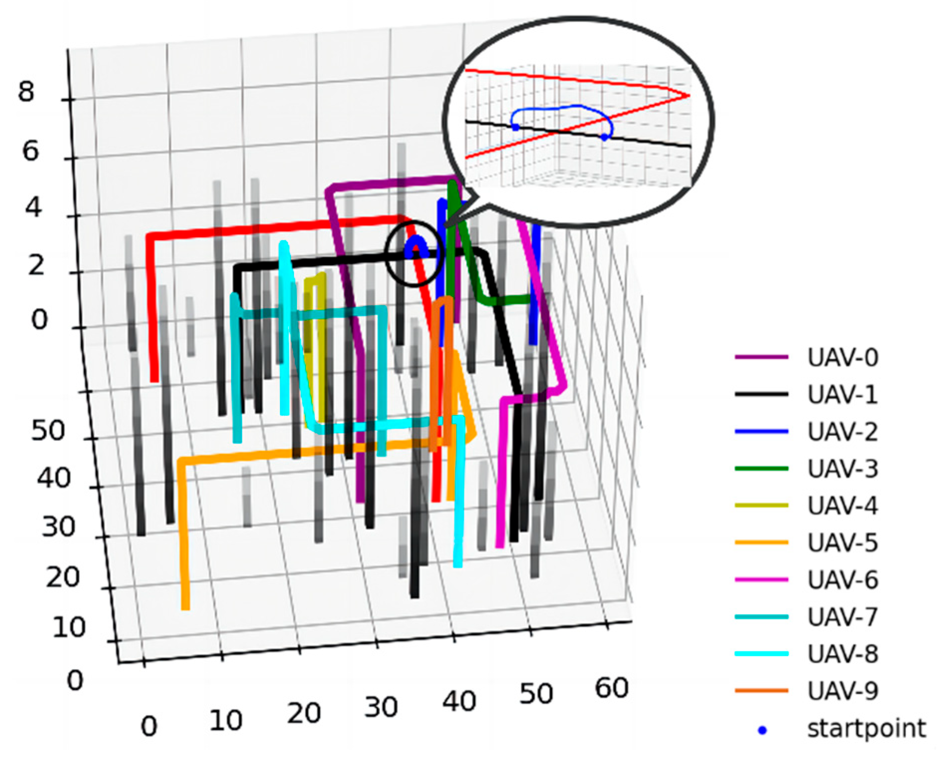
The multi-UAV trajectories obtained using the two-stage air logistics transportation trajectory planning algorithm proposed in this paper are shown in Figure 10. When a non-collaborative target, denoted as UAV-10, appears in the environment, the schematic diagram illustrating the presence of UAVs in the environment during flight is presented in Figure 11. The trajectories of UAV-10 and UAV-1 within the circle in Figure 10 conflict. Therefore, UAV-1 needs to carry out trajectory replanning using NCLPM, as indicated by the blue trajectory in the figure. It can be observed that the replanned trajectory is significantly distant from the original conflicting waypoints, successfully completing the trajectory replanning process.

Assuming that the replanning process for the conflicting trajectories of UAV-1 and UAV-10 does not consider the expected arrival time of UAV-1 to reach the replanning target point, the subsequent flight trajectory of UAV-1 will have a secondary conflict with the remaining UAVs, while Figure 10 shows the time of each waypoint after the algorithm of this chapter considers the ETA replanning, and it can be seen that there is no possibility of secondary conflict between the subsequent trajectory of UAV-1 and the remaining UAVs. In Figure 11, it is illustrated how re-planning avoids secondary conflicts in a multi-drone scenario.

As shown in

Table 5. Comparison of planning times at different resolutions.

Grid Size	Proposed Method Planning Time	A* Planning Time	CFA* Planning Time
85 m × 85 m × 3.4 m	0.0082 s	0.0089 s	0.0092 s
60 m × 60 m × 2.4 m	0.0121 s	0.0115 s	0.0105 s
50 m × 50 m × 2 m	0.0530 s	0.0137 s	0.0140 s
40 m × 40 m × 1.6 m	0.0812 s	0.0154 s	0.0190 s
30 m × 30 m × 1.2 m	0.1325 s	0.0207 s	0.0250 s

, when only considering the global planning stage, the experiment varied the resolution of the map, and the experimental data indicate that the planning time increases with the improvement of resolution, but it remains within an acceptable range, and performance bottlenecks are not encountered under conventional grid sizes.

6.5. Real-World Case with Disturbance Factors

To validate the robustness of the proposed algorithm under real-world environments, we simulated the interferences that UAVs may encounter in real-world environments, including wind and sensor-induced errors.

In the local planning stage, we designed a scenario that generates winds of random magnitudes and directions at random time intervals to mimic wind disturbances, while also adding Gaussian noise to the trajectory to simulate sensor errors.

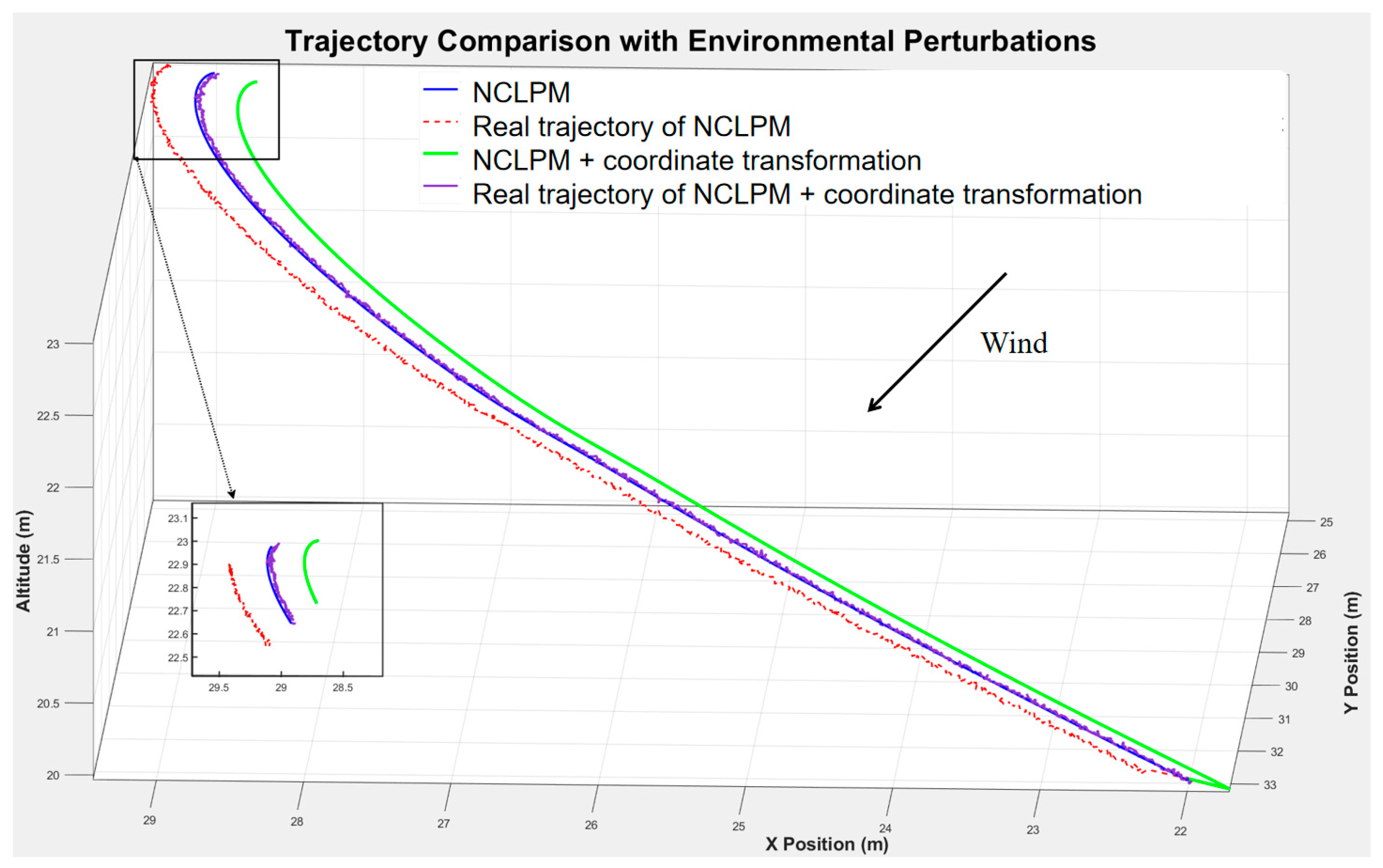
Due to wind interference, the trajectory deviates from the original trajectory without considering any interference. To eliminate this effect, we applied a simple trick through coordinate transformation, and the trajectory can correct the errors caused by wind. For example, as shown in Figure 12, there are four trajectories: the blue line represents the trajectory of vanilla NCLPM, and this curve, when subjected to both wind disturbance and Gaussian noise in the actual environment, results in the red line. To eliminate the effect of wind disturbance, we translated the endpoint in the direction opposite to the wind by multiplying it with the duration of the wind, yielding the corrected trajectory, which is the green line. When the green line is subjected to wind disturbance in the actual environment, it will deviate accordingly, resulting in the purple line. At this point, the trajectory of the purple line has corrected the deviation caused by the wind.

As shown in

Table 6. Evaluation indicators for comparative experiments involving different interference factors.

Metric	NCLPM	Real Trajectory of NCLPM	Real Trajectory of NCLPM + Coordinate Transformation
Time (s)	0.9533	1.4817	0.9608
Distance (m)	11.4399	17.7807	11.5296
ETA deviation (s)	0.0502	×	0.0427

, the real trajectory of NCLPM cannot reach the designated destination due to deviation. Therefore, the corresponding ETA deviation cannot be calculated and is represented as ‘×’ in the table. However, after correcting for wind disturbance using coordinate transformation, the real trajectory of NCLPM is able to reach the destination, and this trajectory is almost identical to that of the vanilla NCLPM. In addition, the deviation in ETA is 0.0427 s, which is almost the same as the 0.0502 s deviation observed in the vanilla NCLPM.

7. Conclusions

This paper proposes a two-stage air logistics transportation trajectory planning method to address the multi-UAV trajectory planning problem in urban VLL logistics scenarios. The original problem is decomposed into a global low-risk trajectory planning problem and a non-secondary conflict local replanning problem, which are solved by RAGPM and NCLPM, respectively. Simulation experiments demonstrate that in global trajectory planning, the ground risk and collision risk have decreased by 80.82%. RAGPM can effectively reduce the collision risk and ground risk of UAVs, enhancing their flight safety. NCLPM can replan conflicting trajectories, and the timing after replanning aligns with the original flight plan; the delay time of NCLPM is also reduced by 99.66–99.9% compared to CFA*, effectively avoiding secondary conflicts. This proves the feasibility of a two-stage air logistics transportation trajectory planning method for multi-UAVs in urban VLL logistics scenarios, providing a safer trajectory solution for UAVs.