A Novel HGW Optimizer with Enhanced Differential Perturbation for Efficient 3D UAV Path Planning

Abstract

In general, path planning for unmanned aerial vehicles (UAVs) is modeled as a challenging optimization problem that is critical to ensuring efficient UAV mission execution. The challenge lies in the complexity and uncertainty of flight scenarios, particularly in three-dimensional scenarios. In this study, one introduces a framework for UAV path planning in a 3D environment. To tackle this challenge, we develop an innovative hybrid gray wolf optimizer (GWO) algorithm, named SDPGWO. The proposed algorithm simplifies the position update mechanism of GWO and incorporates a differential perturbation strategy into the search process, enhancing the optimization ability and avoiding local minima. Simulations conducted in various scenarios reveal that the SDPGWO algorithm excels in rapidly generating superior-quality paths for UAVs. In addition, it demonstrates enhanced robustness in handling complex 3D environments and outperforms other related algorithms in both performance and reliability.

1. Introduction

Unmanned aerial vehicles (UAVs), as modern aerial equipment, have found widespread use in various applications [1,2]. Driven by rapid technological developments in areas such as artificial intelligence, sensor technology, and communication systems, UAVs are now capable of performing increasingly dangerous and complex tasks. These include critical missions such as conducting surveillance in hostile territories, engaging targets with precision, and executing search-and-rescue missions [3,4,5]. To effectively and reliably execute these diverse missions, UAVs must achieve high levels of performance, encompassing key aspects such as autonomy, safety, efficiency, and mission success. Among these enabling technologies driving enhanced UAV performance, path planning stands out as particularly critical. Effective path planning algorithms are essential to ensure that UAVs can navigate autonomously, avoid obstacles, reach their destinations efficiently, and ultimately, accomplish their intended missions successfully, thus garnering significant attention from researchers and practitioners alike.

UAV path planning involves designing a viable route from a start position to a designated destination, while accommodating diverse environmental and mission limitations [6,7]. Particularly in intricate three-dimensional environments, this process poses a complex optimization challenge [8,9,10]. In summary, as the operational area expands and the number of drones increases, the challenge of identifying optimal routes becomes more complex [11,12,13]. Therefore, to enhance the performance of unmanned systems, it is vital to develop effective methods for addressing UAV path planning.

In recent years, scholars have conducted numerous valuable studies and introduced various approaches to address the challenges of path planning, aiming to ensure a safe operating environment. Classical approaches, such as Voronoi diagram (VD) [14], probabilistic roadmaps (PRMs) [15], and rapid-exploring random trees (RRTs) [16], are examples of simple path planning techniques. However, as the scale of the planning problem increases, these methods struggle to estimate a feasible flyable path. Heuristic approaches, including A-star (A*) [17], greedy algorithm [18], and their variants, are also commonly used for path planning due to their good real-time performance. Unfortunately, these methods tend to get trapped in local optima when faced with complex environmental conditions and constraints. Additionally, various metaheuristic algorithms have been introduced to tackle the path planning challenge. Prominent examples encompass ant colony optimization (ACO) [19], particle swarm optimization (PSO) [20], gray wolf optimizer (GWO) [21], and differential evolution (DE) [22]. Such methods are known for their straightforward structure, adaptability, and ease of implementation. They are generally capable of generating feasible flight paths for UAVs that satisfy predefined criteria while operating within constrained computational resources. Despite these advantages, metaheuristic algorithms often encounter the problem of getting stuck in local minima, which means that achieving the optimal solution is not always assured. Lastly, the efficiency of the aforementioned methods has been enhanced by hybridizing two or more algorithms to better estimate a feasible flight path [23,24]. By maximizing the strengths of each single-mode algorithm while minimizing its weaknesses, the performance of these methods is significantly improved. Notable examples include hybrid PSO and coyote optimization (HCPSOA) algorithm [25], hybrid PSO (SDPSO) algorithm [26], and hybrid modified symbiotic organisms search and GWO (HSGWO-MSOS) algorithm [27].

Against this background, metaheuristic algorithms have experienced rapid evolution, primarily due to their inherent simplicity and flexibility [28,29]. By emulating nature processes, these algorithms can effectively navigate complex and expansive solution spaces without relying on detailed problem-specific information. This characteristic enables them to address a diverse array of challenges and renders them indispensable tools for solving intricate optimization problems and enhancing operational efficiency. For example, metaheuristic approaches have been successfully implemented in areas such as vehicle scheduling and system optimization design [30,31], where they contribute significantly to reducing costs and improving operational performance.

The GWO algorithm, proposed by Mirjalili in 2014 [32], is a relatively novel metaheuristic approach that imitates the social behavior and hunting tactics of gray wolves, providing superior exploitation ability and fast convergence. GWO has attracted significant attention and has been employed to address various engineering tasks and control issues [33,34,35,36]. For instance, GWO has shown its effectiveness in areas such as optimal feature selection [37,38], engineering design [39], and neural network training [40]. However, the GWO algorithm still has some defects, such as poor convergence accuracy, a tendency to become trapped in local optima with complex spaces, and challenges in balancing exploration and exploitation [41,42]. To enhance GWO’s performance, researchers have hybridized GWO with other algorithms to develop new hybrid approaches for addressing a path planning problem. Recently, Yu et al. introduced a hybrid GWO method for UAV navigation, which showcased enhanced efficacy and yielded more streamlined, direct paths compared with the traditional GWO algorithm [43]. Similarly, Qu et al. devised an innovative reinforcement learning-based GWO variant, RLGWO, designed for high-quality UAV path planning, which proved effective through simulation experiments [44].

Based on the above considerations, our research targets UAV path planning in 3D environments with various constraints. To address the defects of GWO, we present a novel hybrid GWO algorithm, the simplified GWO with differential perturbation (SDPGWO) algorithm. The proposed algorithm rapidly generates superior routes for UAVs and demonstrates enhanced resilience in intricate operational settings. The key contributions of this work can be summarized as follows:

(1)

A novel SDPGWO algorithm has been developed to address the challenges of 3D UAV path planning.

(2)

The SDPGWO algorithm simplifies GWO to decrease computational complexity and incorporates a differential perturbation strategy to boost its global search capabilities.

(3)

The efficacy of our proposed algorithm for 3D UAV path planning is demonstrated through simulations, which show its superior performance compared with other related algorithms.

The remainder of this article is outlined as follows: Section 2 describes the mathematical model for UAV path planning. Section 3 introduces the SDPGWO algorithm. Experimental results for diverse scenarios are presented in Section 4. Finally, Section 5 provides detailed conclusions.

Notations: Let “$A=:X$” or “$X:=A$” represent “A is defined as X”. The superscript T represents the transpose of a matrix/vector. The 2-norm of vector $\overrightarrow{x}$ is defined by $\parallel \overrightarrow{x}\parallel$.

2. UAV Path Planning

2.1. Problem Description

Path planning is crucial for determining viable routes for UAVs across diverse and complex missions. The main goal is to determine the optimal route for every drone while minimizing the overall path cost. This involves several key components: the UAV itself, the surrounding environment, cost considerations, and mission objectives [45,46]. In addition, one assumes that each aircraft maintains a uniform velocity throughout the mission duration.

In the scenario shown in Figure 1, $C_g-OXYZ$ denotes the global coordinate system, with the origin O positioned at a defined ground position, and the X, Y, and Z axes forming three orthogonal directions. We suppose that the UAV flies from the initial location $S:{(x_s,y_s,z_s)}^{\mathrm{T}}$ to the destination $T:{(x_t,y_t,z_t)}^{\mathrm{T}}$. Mountain peaks, radar installations, and other dangerous zones are considered inaccessible for UAVs. These regions, known as obstacle zones, significantly impact UAV flight safety and directly affect the effectiveness of planned routes. We assume that the locations and dimensions of all obstacles are predetermined. Let $O_i$, where $(i=1,2,\cdots ,M)$, denote these threats, with M indicating the total count of threats.

2.2. Path Representation

The flight path consists of N waypoints besides S and T. The path is represented as $P_{\mathrm{UAV}}=\{S,p_1,\cdots p_N,T\}$, where each waypoint $p_j:{(x_j,y_j,z_j)}^{\mathrm{T}}$ for $j\in [1,N]$ serves as a control point. To simplify the modeling process, let $p_0:=S$, $p_{N+1}:=T$, and denote ${\overrightarrow{L}}_k:={(x_{k+1}-x_k,y_{k+1}-y_k,z_{k+1}-z_k)}^{\mathrm{T}}$, $k=0,1,\cdots ,N$ as the path segment vector between the waypoints $p_k$ and $p_{k+1}$.

We project the points S and T onto the $OXY$ plane, resulting in $S^{\prime }:{(x_s,y_s,0)}^{\mathrm{T}}$ and $T^{\prime }:{(x_t,y_t,0)}^{\mathrm{T}}$, as shown in Figure 2. To enhance search efficiency and reduce dimensional complexity, we introduce a rotated coordinate frame $C_r-O^{\prime }{X}^{\prime }{Y}^{\prime }{Z}^{\prime }$. The origin $O^{\prime }$ is positioned at $S^{\prime }$, and the new X-axis aligns with $S^{\prime }{T}^{\prime }$. Let L represent the distance between $S^{\prime }$ and $T^{\prime }$. In the $C_r$ system, the start and target points are $S_r:{(0,0,z_s)}^{\mathrm{T}}$ and $T_r:{(L,0,z_t)}^{\mathrm{T}}$. The line segment $S^{\prime }{T}^{\prime }$ is then divided into $N+1$ equidistant segments by N vertical lines, denoted as $l_1,l_2,\cdots ,l_N$. The distance between these lines is given by $\Delta l=L/(N+1)$. Any point situated on the $k^{th}$ line, $l_k$, in the $C_r$ frame, will share a common horizontal coordinate $x_k^r=k\Delta l,k=1,2,\cdots ,N$.

Figure 1. Example of 3D environment for UAV path planning.

Figure 1. Example of 3D environment for UAV path planning.

In three-dimensional space, these N lines correspond to N planes that are parallel and perpendicular to $OXY$. Thus, we select N discrete points ${(x_j^r,y_j^r,z_j^r)}^{\mathrm{T}},j=1,2,\cdots ,N$, on these planes as waypoints and only need to determine the $y_j^r$ and $z_j^r$ coordinates for each point in the $C_r$ system. This approach converts the 3D path planning challenge into a 2D problem, thereby greatly reducing processing overhead. The transformation between two reference systems is carried out as follows:

$$\begin{array}{c}\hfill \left[\begin{array}{c}x\\ y\\ z\end{array}\right]=\left[\begin{array}{ccc}cos\theta & -sin\theta & 0\\ sin\theta & cos\theta & 0\\ 0& 0& 1\end{array}\right]·\left[\begin{array}{c}{x}_r\\ y_r\\ z_r\end{array}\right]+\left[\begin{array}{c}{x}_s\\ y_s\\ 0\end{array}\right],\end{array}$$

(1)

where ${(x,y,z)}^{\mathrm{T}}$ and ${(x_r,y_r,z_r)}^{\mathrm{T}}$ denote the coordinates of an identical point as expressed in the original frame $C_g$ and the rotated frame $C_r$, respectively. The rotation angle, $\theta$, is defined as the angle formed between the X axis of the original frame and the rotated segment $S^{\prime }{T}^{\prime }$.

2.3. Objective Function

In the earlier description, our goal is to identify the most efficient route for the UAV within the framework of path planning. To achieve this objective, we evaluate the path using an overall objective function, which is composed of three sub-functions: path length cost, path altitude cost, and path threat cost. The corresponding cost functions are as follows:

(1) Path length cost

Since UAVs have limited fuel, selecting a shorter path reduces fuel consumption and decreases the likelihood of encountering unexpected threats. $J_L$, the cost for path length, is simply the total UAV path distance, calculated by the following:

$$\begin{array}{cc}\hfill J_L\left(\mathit{x}\right)& :=\sum _{i=0}^N\parallel {\overrightarrow{L}}_i\parallel ,\hfill \end{array}$$

(2)

$$\begin{array}{cc}\hfill \parallel {\overrightarrow{L}}_i\parallel & =\sqrt{{(x_{i+1}-x_i)}^2+{(y_{i+1}-y_i)}^2+{(z_{i+1}-z_i)}^2},\hfill \end{array}$$

(3)

where $\mathit{x}$ represents the UAV path matrix, $\mathit{x}:=[p_0,p_1,\cdots p_N,p_{N+1}]$.

(2) Path altitude cost

In 3D route planning, higher flight altitudes make UAVs more susceptible to enemy radar, while lower flight altitudes increase the risk of ground collisions. Furthermore, minimizing altitude changes during flight is crucial for maintaining energy efficiency. The cost function $J_H$ represents the UAV’s altitude changes during flight and can be computed as follows:

$$\begin{array}{cc}\hfill & Cos{t}_i:=\left\{\begin{array}{cc}\hfill \left|z_{i+1}-z_i\right|,\mathrm{if}& z_{min}⩽z_i,z_{i+1}⩽z_{max},\hfill \\ \hfill \infty ,& \mathrm{otherwise},\hfill \end{array}\right.\hfill \end{array}$$

(4)

$$\begin{array}{cc}\hfill & J_H\left(\mathit{x}\right):=\sum _{i=0}^{N}Cos{t}_i,\hfill \end{array}$$

(5)

where $z_{min}$ and $z_{max}$ are the UAV’s lowest and highest allowed flight levels.

(3) Path threat cost

In the UAV flight path, if a path segment $L_k$ intersects with a threat, that segment is considered to be affected by the threat. Denote the M threats in the environment as $O_1$, $O_2$, ⋯, $O_j$, ⋯, $O_M$, and use $L_k\cap O_j$ to represent the path segment $L_k$ being affected by $O_j$. The threat cost $w_{L_k}$ of a path segment $L_k$ is defined as follows:

$$\begin{array}{cc}\hfill & w_{L_k}:={\displaystyle \frac{\parallel {\overrightarrow{L}}_k\parallel }{5}}\sum _{j=1}^M{D}_j,\hfill \end{array}$$

(6)

$$\begin{array}{cc}\hfill & D_j:=\left\{\begin{array}{c}\hfill P\times L_{kj},L_k\cap O_j,\\ \hfill 0,\mathrm{otherwise},\end{array}\right.\hfill \end{array}$$

(7)

where in $L_{kj}$ denotes the path segment length $L_k$ that traverses that threat $O_j$, and P signifies the penalty coefficient.

The cost function $J_T$ related to path threats is defined as follows:

$$\begin{array}{c}\hfill J_T\left(\mathit{x}\right):=\sum _{k=0}^N{w}_{L_k}=w_{L_0}+w_{L_1}+\cdots +w_{L_N}.\end{array}$$

(8)

(4) Overall objective function

The overall objective function, denoted as $J\left(\mathit{x}\right)$, employed for the comprehensive evaluation of a UAV’s path, is expressed as follows:

$$J\left(\mathit{x}\right)=v_1·J_L\left(\mathit{x}\right)+v_2·J_H\left(\mathit{x}\right)+v_3·J_T\left(\mathit{x}\right),$$

(9)

where $v_i(i=1,2,3)$ denotes the relative weight factors that satisfy $v_1+v_2+v_3=1$. The value of $v_i$ should be modified according to the specific scenario.

2.4. Path Smoothing

Typically, paths generated by metaheuristic algorithms consist of many line segments. To achieve a smooth and feasible trajectory, the cubic B-spline technique is employed. The B-spline improves upon the Bezier curve by overcoming limitations like the higher polynomial degree with additional points and the curve’s sensitivity to control point adjustments.

Let $q_i(i=0,1,\cdots ,n)$ denote the control points and $N_{i,k}\left(u\right)$ be the k-order normalized B-spline basis functions, defined by the following recursive Cox–deBoor formulas:

$$\left\{\begin{array}{c}{N}_{i,1}\left(u\right)=\left\{\begin{array}{c}1,\mathrm{if}{u}_i⩽u⩽u_{i+1}\hfill \\ 0,\mathrm{otherwise}\hfill \end{array}\right.\hfill \\ N_{i,k}\left(u\right)={\displaystyle \frac{u-u_i}{u_{i+k-1}-u_i}}{N}_{i,k-1}\left(u\right)+{\displaystyle \frac{u_{i+k}-u}{u_{i+k}-u_{i+1}}}{N}_{i+1,k-1}\left(u\right),k>1\hfill \end{array}\right.$$

(10)

The B-spline curves are then represented by Equation (11).

$$P\left(u\right)=\sum _{i=0}^n{q}_i{N}_{i,k}\left(u\right).$$

(11)

The constituent basis functions, $N_{i,k}\left(u\right)$, are constructed based on a non-decreasing sequence of parameters termed parametric knots, denoted as $\{u_0⩽u_1⩽\cdots ⩽u_{k+n}\}$. Additionally, each basis function $N_{i,k}\left(u\right)$ is a piecewise polynomial within a defined interval and satisfies ${\sum }_{i=0}^k{N}_{i,n}\left(t\right)\equiv 1$.

3. Improved Gray Wolf Optimizer Algorithm

The ensuing section delineates the fundamental principles and process of the standard GWO. Building on its characteristics, we present an enhanced variant that overcomes the limitations of the original GWO and effectively tackles the UAV path planning challenge.

3.1. Standard GWO Algorithm

The GWO algorithm draws inspiration from the social structure and hunting behavior of gray wolves, which are classified into four types: $\alpha$, $\beta$, $\delta$, and $\omega$. The $\alpha$, $\beta$, and $\delta$ wolves are considered the leader wolves, guiding the base pack of $\omega$ wolves [47]. In the GWO algorithm, each agent’s spatial location is treated as a candidate solution within the solution space of the optimization problem.

The core operation of the GWO algorithm comprises two phases. The initial phase involves surrounding the pray, while the subsequent phase focuses on attacking it. In the first phase, gray wolves surround the prey, a behavior described as follows:

$$\begin{array}{cc}\hfill D& =|C\times X_p\left(t\right)-X\left(t\right)|,\hfill \end{array}$$

(12)

$$\begin{array}{cc}\hfill X(t+1)& =X_p\left(t\right)-A\times D,\hfill \end{array}$$

(13)

where t indicates the current iteration number, X is the wolf’s position, and $X_p$ is the prey’s position. The coefficient parameters A and C are shown as follows:

$$\begin{array}{cc}\hfill A& =2a\times r_1-a,\hfill \end{array}$$

(14)

$$\begin{array}{cc}\hfill C& =2\times r_2,\hfill \end{array}$$

(15)

$$\begin{array}{cc}\hfill a& =2-2t/t_{max},\hfill \end{array}$$

(16)

where $r_1$ and $r_2$ are random values in the range [0, 1]. The parameter a is linearly reduced from 2 to 0.

In the subsequent phase, the wolves, led by $\alpha$, $\beta$, and $\delta$, proceed to hunt the prey by updating their positions. The specific mathematical equations are given below:

$$\begin{array}{cc}\hfill D_{\alpha }& =\left|C_1\times X_{\alpha }-X\right|,\hfill \end{array}$$

(17)

$$\begin{array}{cc}\hfill D_{\beta }& =\left|C_2\times X_{\beta }-X\right|,\hfill \end{array}$$

(18)

$$\begin{array}{cc}\hfill D_{\delta }& =\left|C_3\times X_{\delta }-X\right|,\hfill \end{array}$$

(19)

$$\begin{array}{cc}\hfill X_1& =X_{\alpha }-A_1\times D_{\alpha },\hfill \end{array}$$

(20)

$$\begin{array}{cc}\hfill X_2& =X_{\beta }-A_2\times D_{\beta },\hfill \end{array}$$

(21)

$$\begin{array}{cc}\hfill X_3& =X_{\delta }-A_3\times D_{\delta },\hfill \end{array}$$

(22)

$$\begin{array}{cc}\hfill X(t+1)& =(X_1+X_2+X_3)/3.\hfill \end{array}$$

(23)

where $X_{\alpha }$, $X_{\beta }$, and $X_{\delta }$ represent the positions of the leader wolves. In Equations (17)–(19), $D_{\alpha }$, $D_{\beta }$, and $D_{\delta }$ are the distance vectors between the search agent and $\alpha$, $\beta$, and $\delta$, respectively. Algorithm 1 shows the pseudocode of GWO.

Algorithm 1 Pseudocode of the GWO method

1: Initialize positions of the gray wolves, $X_i$ for $i=1,\cdots ,P$  2: Compute the fitness $f\left(X_i\right)$  3: Find the $\alpha$, $\beta$, and $\delta$ wolves based on fitness values  4: Set initial values for A, C, a, and $t_{max}$  5: while$t<t_{max}$ do  6:       for $i=1:P$ do  7:             Update $X_i$ wolves using Equations (17)–(23)  8:       end for  9:       Adjust A, C, and a according to Equations (14)–(16) 10:       Recalculate the fitness of all search agents 11:       Update $X_{\alpha }$, $X_{\beta }$, and $X_{\delta }$ 12: end while 13: Return $X_{\alpha }$

3.2. The Proposed SDPGWO Algorithm

As discussed in Section 3.1, the traditional GWO algorithm is straightforward and simple to execute. However, like many metaheuristic algorithms, the standard GWO, when applied to complex optimization problems, may still encounter challenges related to high computational cost and susceptibility to premature convergence and entrapment in local optima. Therefore, to enhance the efficiency of the GWO algorithm in solving complex problems while reducing its computational burden, we simplified the standard GWO’s update mechanism and proposed the SDPGWO algorithm. The SDPGWO algorithm achieves simplification by concentrating the guidance of individual wolf updates on the alpha wolf, thereby maximizing the retention of the original GWO algorithm’s inherent excellent exploitation capability. Simultaneously, we further leverage a differential perturbation strategy to augment the diversity of solutions.

(1) Simplification strategy

In the standard GWO, the top 3 wolves each hold distinct social roles, with the $\alpha$ wolf leading the pack. To enhance GWO’s search efficiency and make better use of the $\alpha$ wolf’s information, we propose a simplification strategy. Rather than relying on the guidance of all three top wolves, individuals update their positions based exclusively on the $\alpha$ wolf. The update equations for the simplified GWO are shown as follows:

$$\begin{array}{cc}\hfill D^{*}& =\left|C^{*}\times X_{\alpha }\left(t\right)-X_i\left(t\right)\right|,\hfill \end{array}$$

(24)

$$\begin{array}{cc}\hfill X_i(t+1)& =X_{\alpha }\left(t\right)-A^{*}\times D^{*},\hfill \end{array}$$

(25)

$$\begin{array}{cc}\hfill A^{*}& =2a\times r_1-a,\hfill \end{array}$$

(26)

$$\begin{array}{cc}\hfill C^{*}& =2\times r_2,\hfill \end{array}$$

(27)

$$\begin{array}{cc}\hfill a& =2-2t/t_{max},\hfill \end{array}$$

(28)

From Equations (24)–(28), only the information of the $\alpha$ wolf is retained in the simplified update equations. This simplification decreases the algorithm’s computational complexity while retaining the excellent exploitation capability of the GWO algorithm. By focusing on the dominant $\alpha$ wolf, we streamline the updating process, making it more efficient without sacrificing the original GWO algorithm’s strengths.

(2) Differential perturbation strategy

Drawing inspiration from the differential mutation process in DE and aiming to enhance GWO’s global search capability, we propose an innovative differential perturbation strategy. In the DE algorithm, the creation of a novel individual is achieved by incorporating a scaled difference vector between two individuals into a third individual. This random perturbation technique markedly enhances population diversity and improves exploration during the initial stages of DE. Consequently, we propose the following differential perturbation strategy:

$$V_i(t+1)=pbes{t}_i\left(t\right)+F_r\times (X_r\left(t\right)-pbes{t}_i\left(t\right)),$$

(29)

where $pbes{t}_i\left(t\right)$ denotes the historical best position of the i-th individual at iteration t, and r is the index of a gray wolf randomly chosen from the current population. The scaling factor $F_r$ is a random number within the range [0, 2].

In Equation (29), the first term on the right-hand side represents the historical optimal location of the i-th individual, while the second term denotes the weighted difference between the randomly selected location of the r-th individual and this historical optimal position. A larger $F_r$ increases the search range, enhancing the global search ability, while a smaller $F_r$ narrows the search range, aiding local search. Thus, this approach balances exploration and exploitation effectively. The random value $F_r$ enhances population diversity, significantly improving the global search capability of GWO in the initial stages.

(3) Hybridizing two strategies

To combine the advantages of both strategies described above, we introduce a hybrid approach by incorporating a greedy selection mechanism. This results in the SDPGWO algorithm, which combines the simplified strategy and the differential perturbation strategy.

In the SDPGWO algorithm, the optimization process is divided into two stages. First, we update the individual positions using Equations (24)–(28) to obtain the current optimal position $pbes{t}_i\left(t\right)$ of each individual in the population by the greedy selection method. The procedure is as follows:

$$pbes{t}_i\left(t\right)=\left\{\begin{array}{c}{X}_i^{\prime }\left(t\right),\mathrm{if}F\left(X_i^{\prime }\left(t\right)\right)⩽F\left(X_i\left(t\right)\right)\hfill \\ X_i\left(t\right),\mathrm{otherwise}\hfill \end{array}\right.$$

(30)

Here, $X_i\left(t\right)$ represents the original solution, while $X_i^{\prime }\left(t\right)$ is the solution obtained by the simplification strategy. Then, we further refine the positions using the differential perturbation strategy. The update is given by the following:

$$X_i(t+1)=\left\{\begin{array}{c}{V}_i(t+1),\mathrm{if}F\left(V_i(t+1)\right)⩽F\left(pbes{t}_i\left(t\right)\right)\hfill \\ pbes{t}_i\left(t\right),\mathrm{otherwise}\hfill \end{array}\right.$$

(31)

Here, $V_i(t+1)$ is the solution obtained using the differential perturbation strategy. Combining the simplification strategy reduces computational complexity while retaining strong exploitation capabilities. Meanwhile, the differential perturbation strategy enhances global search ability and maintains population diversity, particularly during the initial stages of the search. This dual-strategy hybridization effectively balances the exploration and exploitation, resulting in more robust and efficient optimization outcomes.

Based on Equation (30), it is observed that $F\left(pbes{t}_i\left(t\right)\right)⩽F\left(X_i\left(t\right)\right)$, and according to Equation (31), we can get that $F\left(X_i(t+1)\right)⩽F\left(pbes{t}_i\left(t\right)\right)⩽F\left(X_i\left(t\right)\right)$. Therefore, $F\left(X_i(t+1)\right)⩽F\left(X_i\left(t\right)\right)$. This shows that the function $F\left(X_i\left(t\right)\right)$ is monotonically non-increasing, which also demonstrates that the quality of the solution is improving through iterative computation.

The pseudocode of SDPGWO is given below in Algorithm 2.

Algorithm 2 Pseudocode of the SDPGWO method

Initial  1: Let $t=1$ and randomly generate initial population positions $X_i(i=1,2,\cdots ,P)$  2: Give the maximum iteration number $t_{max}$ and individual dimension $Dim$  3: Compute the fitness $f\left(X_i\right)$ and select $X_{\alpha }$ Optimize  4: while$t<t_{max}$ do  5:       Calculate a, $A^{*}$, $C^{*}$ by Equations (26)–(28)  6:       for $i=1$: P do  7:               Calculate $X_i^{\prime }\left(t\right)$ by (24)–(25)  8:               Update $pbes{t}_i\left(t\right)$ by the greedy selection between $X_i^{\prime }\left(t\right)$ and $X_i\left(t\right)$  9:               Calculate $V_i(t+1)$ by (29) 10:               Update $X_i(t+1)$ by the greedy selection between $V_i(t+1)$ and $pbes{t}_i\left(t\right)$ 11:       end for 12:       Correct out-of-bounds agents 13:       Re-evaluate the fitness $f\left(X_i\right)$ 14:       Update $X_{\alpha }$ 15: end while 16: Return $X_{\alpha }$

3.3. Application of SDPGWO in UAV Path Planning

In this subsection, we detail the steps for UAV path planning using the SDPGWO method. The detailed procedure is summarized below.

• Define the UAV flight scenario in 3D space. Load UAV mission parameters and environmental information, including the waypoints, the UAV’s initial and target positions, obstacle positions, and the flight constraints.
• Initialize UAV flight path information. First, transform the coordinate system according to Equation (1). In the new coordinate system, randomly assign initial positions to the gray wolf population, which will represent the initial trajectory of the UAV. Calculate the fitness value of each individual using the objective function $J\left(\mathit{x}\right)$, and select the best individual to set as $X_{\alpha }$.
• Optimize the model. Utilize the SDPGWO algorithm to optimize the model. During each iteration, evaluate the cost of each potential solution using Equations (2)–(9). Concurrently, update the candidate solutions according to Algorithm 2 of the SDPGWO method.
• Output the optimal solution. Once the algorithm reaches the maximum iteration limit, conclude the search process and present the best solution found. Otherwise, if the maximum iteration limit has not been reached, the algorithm returns to Step 3 to continue the optimization process.
• Coordinate system inverse transformation. Apply the coordinate system inverse transformation to the optimal path obtained in Step 4. Perform a smoothing operation on the transformed path to generate the final UAV flight path.

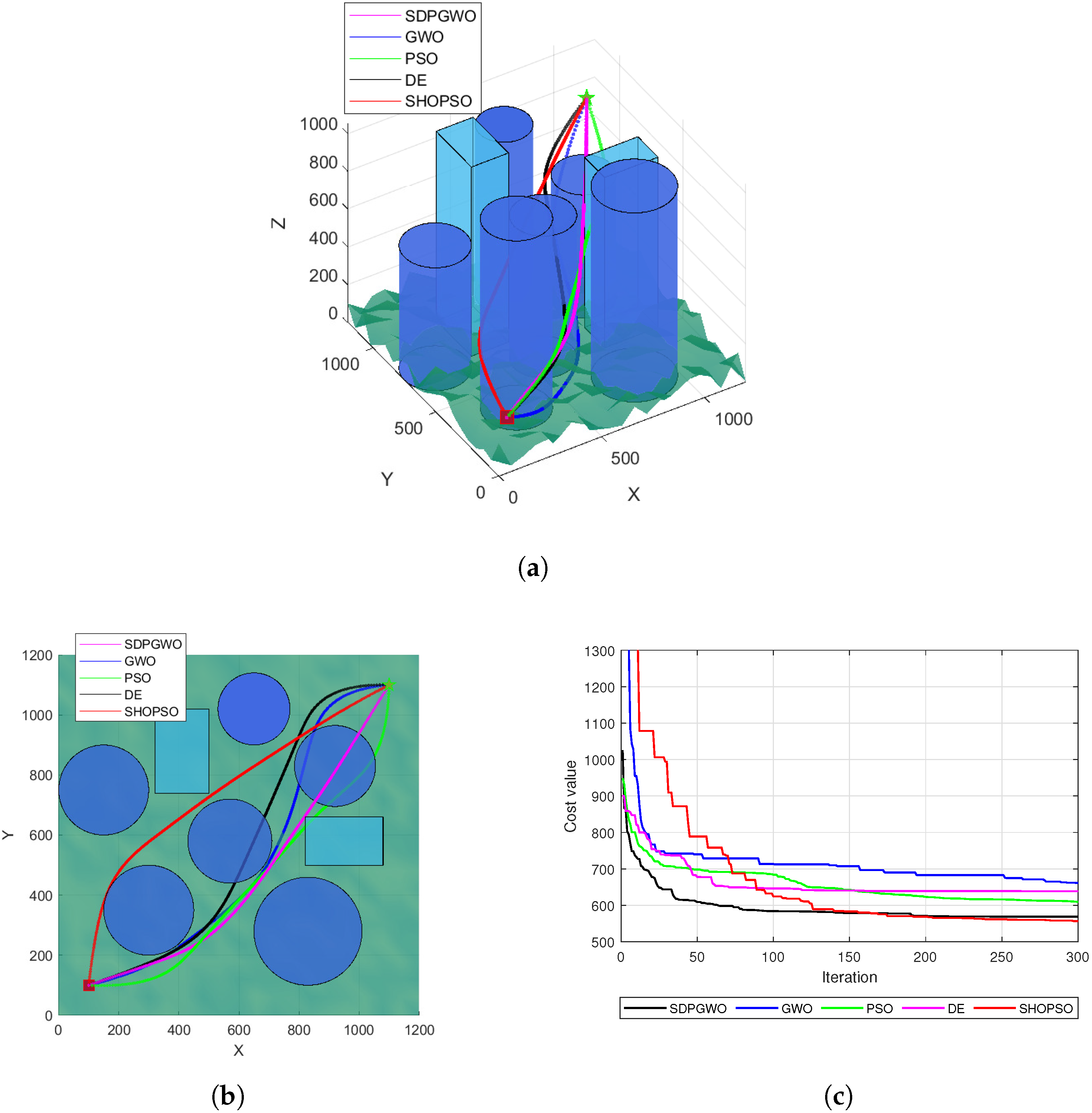
4. Simulation Example

In this section, we model the UAV as a point object to evaluate the effectiveness of the SDPGWO algorithm in generating optimal routes in a 3D environment. The threats within the planning area are modeled as cylinders and cuboids. Two maps are used for this purpose, with details provided in

Table 1. Obstacle information.

Obstacle	Map 1		Map 2
	Threat Location	Height	Threat Location	Height
Cylinders	(200, 720, 120)	800	(150, 750, 150)	650
	(850, 800, 120)	1000	(920, 830, 135)	650
	(300, 330, 130)	250	(300, 350, 150)	1000
	(650, 480, 140)	750	(570, 580, 140)	750
	NA	NA	(830, 280, 180)	1000
	NA	NA	(650, 1020, 120)	900
Cuboids	(650, 90)–(950, 270)	900	(820, 500)–(1080, 660)	900
	(410, 810)–(590, 1090)	1000	(320, 740)–(500, 1020)	1000

. To validate the performance of the SDPGWO algorithm, we include comparative results with both traditional and recently developed methods, including GWO, PSO, DE, and the hybrid method of selfish herd optimizer and PSO (SHOPSO) [23]. The entire simulation suite was executed using MATLAB R2022a operating on a Windows 10 system.

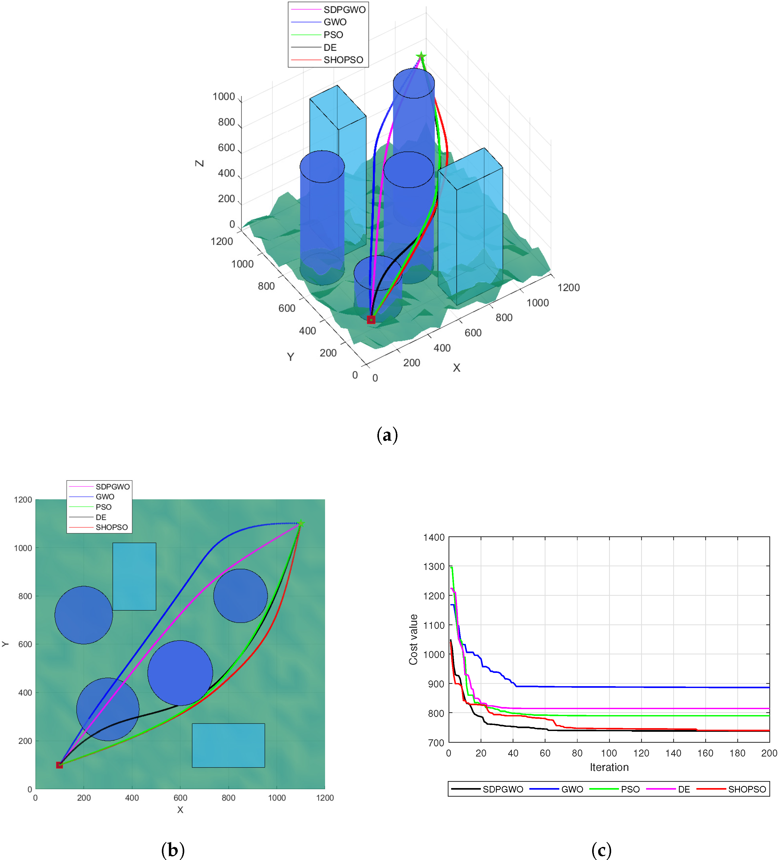
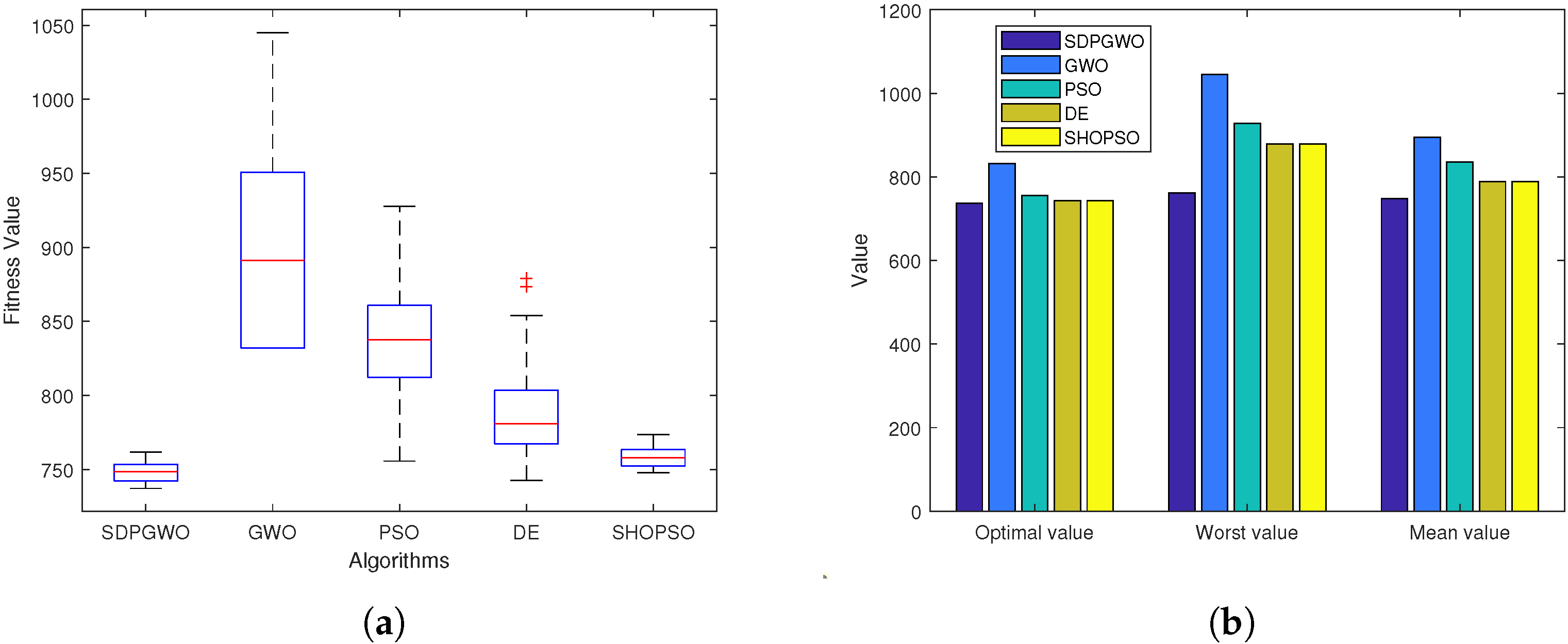
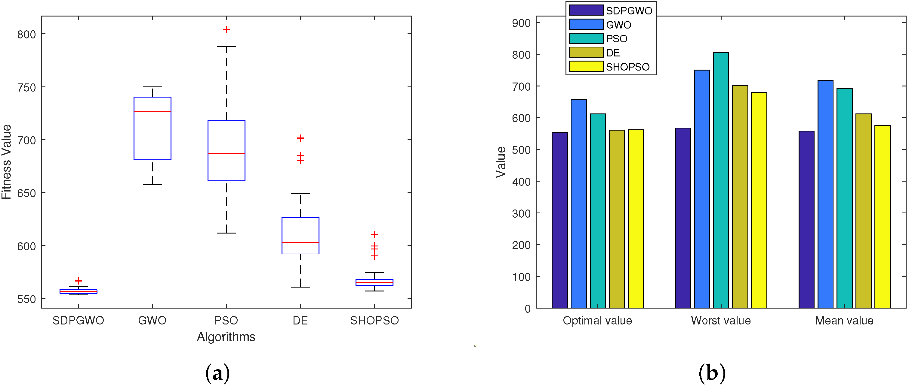
4.1. Experimental Results in Map 1

In this scenario, the SDPGWO algorithm, alongside other mentioned optimization methods, serves to find the best path in a 3D environment from $S(100,100,200)$ to $T(1100,1100,800)$. The algorithm parameters are detailed in

Table 2. Algorithm parameter setting.

Algorithm	Parameter
DE	$F_r=0.5$, $CR=0.9$
PSO	$c_1=c_2=1.5$, $w:0.4\sim 0.9$
GWO	$a=2\sim 0$
SHOPSO	$a=1\sim 0$, $\omega =0.75$, $c_1=c_2=2$
SDPGWO	$a=2\sim 0$, $F_r:0\sim 2$

. To ensure experimental fairness, all algorithms set the population size to 50. We compared these algorithms using different numbers of waypoints (n), including $n=8,10,12$, to evaluate the search ability and scalability of algorithms. All the experiments are executed independently 50 times, and the maximum number of iterations was set to 200.

Figure 3a illustrates the optimal UAV paths produced by the five algorithms for $n=8$, with a top view in Figure 3b. Analysis reveals that both the GWO and DE algorithms failed to successfully generate feasible paths, while the remaining three algorithms effectively avoided all threats. Among the viable paths, SDPGWO produced the most efficient path with the shortest length. Further, the convergence curves of the fitness function for each algorithm, displayed in Figure 3c, indicate that SDPGWO achieves the lowest fitness value, confirming its superiority. SDPGWO also exhibits rapid convergence, reaching the global minimum within 40 iterations, a rate faster than that achieved by PSO, GWO, DE, and SHOPSO. Although the DE algorithm converges quickly, it clearly falls into local optima. This underscores SDPGWO’s effectiveness in achieving both rapid convergence and robust global optimization performance.

Figure 4a shows the optimal UAV paths generated by the five algorithms for $n=10$, with a top view in Figure 4b. A closer examination reveals that only the GWO and PSO algorithms failed to find feasible solutions. In contrast, the DE, SHOPSO, and SDPGWO algorithms all successfully generated feasible paths that avoid the boundaries of all threats. However, the path generated by DE exhibited a higher curvature, leading to increased path length and reduced fuel efficiency. The SDPGWO algorithm outperformed the DE algorithm, generating a more direct and efficient path. The SHOPSO algorithm also demonstrated excellent performance, with its generated path length only second to the SDPGWO algorithm and superior to the DE and PSO algorithms. Figure 4c presents the convergence curves for all five algorithms and clearly shows SDPGWO achieving the lowest cost function value, significantly outperforming the SHOPSO, GWO, PSO, and DE algorithms. The GWO and PSO algorithms fall into local optima prematurely. On the other hand, SDPGWO reaches the global minimum within 60 iterations, whereas DE falls into a local minimum after 90 iterations. This verifies that SDPGWO begins converging early and consistently achieves the global optimal path with greater stability.

Figure 5a shows the optimal UAV paths produced by the five different algorithms discussed for $n=12$, with a top view in Figure 5b. The SDPGWO algorithm produced a path that is not only excellent in flight altitude but also the smoothest among all. In contrast, the PSO, GWO, and DE paths exhibited oscillatory behavior. Furthermore, the PSO path failed to avoid obstacles, and the GWO path was notably more curved and longer. The path generated by DE had a higher altitude, which was also unfavorable for UAV flight. SHOPSO generated a path that was smoother than that of PSO, GWO, and DE but less smooth than that of SDPGWO. Figure 5c shows convergence curves for the five algorithms. SDPGWO demonstrated superior convergence accuracy, achieving the lowest cost function value. SHOPSO followed SDPGWO with the second-best convergence, outperforming DE, PSO, and GWO. While DE achieved satisfactory accuracy after approximately 150 iterations, SDPGWO achieved the same level within just 40 iterations, and SHOPSO in slightly more iterations than SDPGWO. Although the PSO and GWO algorithms demonstrate faster convergence in the early stages, they prematurely fall into local optima, resulting in suboptimal convergence performance.

Table 3. Comparison of statistical performance metrics of algorithms (50 runs).

Case	Indicators	SDPGWO	SHOPSO	GWO	PSO	DE
$n=8$	Optimal	$7.3815\times {10}^2$	$7.3850\times {10}^2$	$8.2267\times {10}^2$	$7.4077\times {10}^2$	$7.3965\times {10}^2$
	Worst	$7.6055\times {10}^2$	$7.8542\times {10}^2$	$1.0079\times {10}^3$	$8.6714\times {10}^2$	$8.2457\times {10}^2$
	Mean	$7.4360\times {10}^2$	$7.4952\times {10}^2$	$8.7095\times {10}^2$	$7.9144\times {10}^2$	$7.5969\times {10}^2$
	Std	$7.7231$	$10.5350$	$55.7512$	$31.3653$	$16.8804$
$n=10$	Optimal	$7.3715\times {10}^2$	$7.3780\times {10}^2$	$8.3199\times {10}^2$	$7.5559\times {10}^2$	$7.4267\times {10}^2$
	Worst	$7.6154\times {10}^2$	$7.9500\times {10}^2$	$1.0451\times {10}^3$	$9.2765\times {10}^2$	$8.7912\times {10}^2$
	Mean	$7.4809\times {10}^2$	$7.5500\times {10}^2$	$8.9523\times {10}^2$	$8.3535\times {10}^2$	$7.8899\times {10}^2$
	Std	$6.8625$	$12.6232$	$69.5763$	$35.6379$	$30.8307$
$n=12$	Optimal	$7.3658\times {10}^2$	$7.3720\times {10}^2$	$8.4001\times {10}^2$	$8.0548\times {10}^2$	$7.5076\times {10}^2$
	Worst	$8.1731\times {10}^2$	$8.3580\times {10}^2$	$1.0532\times {10}^3$	$9.8127\times {10}^2$	$9.2529\times {10}^2$
	Mean	$7.6768\times {10}^2$	$7.8500\times {10}^2$	$9.2545\times {10}^2$	$8.9289\times {10}^2$	$8.2058\times {10}^2$
	Std	$16.9640$	$20.5662$	$62.0516$	$36.9430$	$37.2342$

presents the experimental results from 50 independent runs of each algorithm across the three cases, including the maximum (Optimal), minimum (Worst), mean (Mean), and standard deviation (Std) of the objective function.

Table 4. Comparison of average performance metrics for five algorithms (50 runs).

Case	Indicators	SDPGWO	SHOPSO	GWO	PSO	DE
$n=8$	Path length	1594.85	1621.37	1683.72	1654.28	1632.72
	Runtime (s)	60.78	72.92	42.48	48.52	52.37
	SR (%)	100.0	100.0	48.0	82.0	96.0
$n=10$	Path length	1598.32	1628.36	1720.52	1673.62	1640.50
	Runtime (s)	65.53	78.29	48.72	51.50	55.41
	SR (%)	100.0	100.0	46.0	64.0	90.0
$n=12$	Path length	1608.80	1630.47	1734.95	1688.26	1645.63
	Runtime (s)	72.37	85.90	53.73	56.30	60.05
	SR (%)	100.0	96.0	32.0	38.0	72.0

shows the average performance metrics obtained by the five algorithms. These metrics include average path length (path length), runtime, and success rate (SR). Here, SR represents the percentage of successful runs achieving feasible paths that satisfy all constraints.

From the results in Table 3 and Table 4 and Figure 6, Figure 7 and Figure 8, SDPGWO demonstrably excels over the other algorithms in nearly all performance aspects. As shown in Table 3, the SDPGWO algorithm achieves the best performance across all scenarios in statistical metrics such as Optimal, Worst, Mean, Std. Moreover, Table 4 highlights SDPGWO’s advantage in average path length and success rate. However, regarding the runtime, the SDPGWO algorithm is not the fastest, but its runtime is not significantly different from that of other algorithms and remains within an acceptable range. Furthermore, the box plots in Figure 6, Figure 7 and Figure 8 reveal that the optimal values obtained by SDPGWO are highly stable, with minimal fluctuations, underscoring its reliability. This stability further confirms that SDPGWO consistently provides safe and efficient path planning for UAVs.

Based on the above experimental results, it is clear that the number of waypoints significantly impacts the optimization performance of the five algorithms under the same conditions. As ‘n’ increases from 8 to 12, the performance of all five algorithms worsens, particularly for GWO, PSO, and DE, whose SR values also decrease, making it harder for them to generate feasible UAV flight paths. This decline in performance is due to the increased dimensionality of the optimization problem, which raises the difficulty of the search and leads to deviations from the optimal solution. Likewise, having too few waypoints can result in paths that lack smoothness and have higher objective function values.

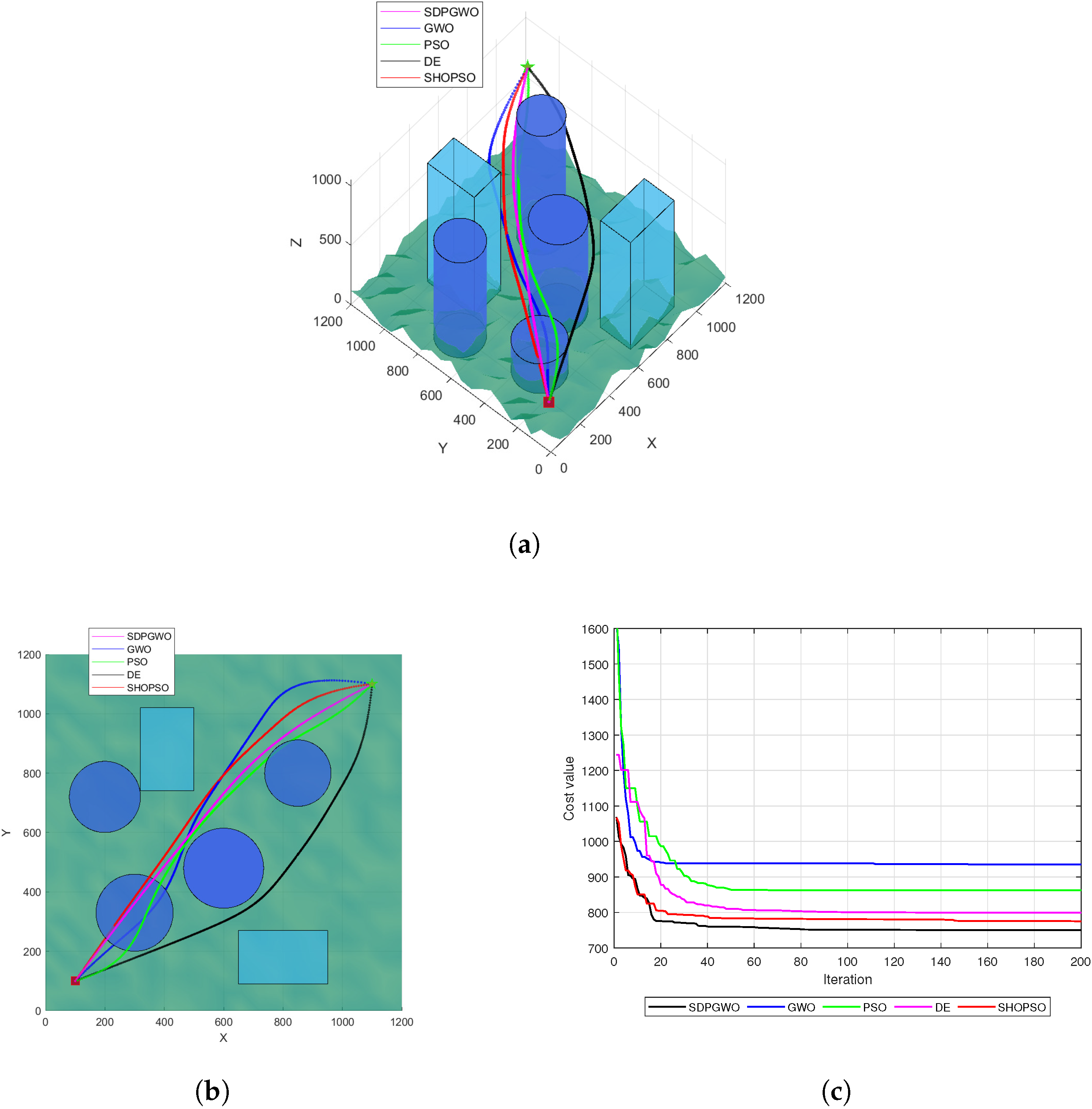
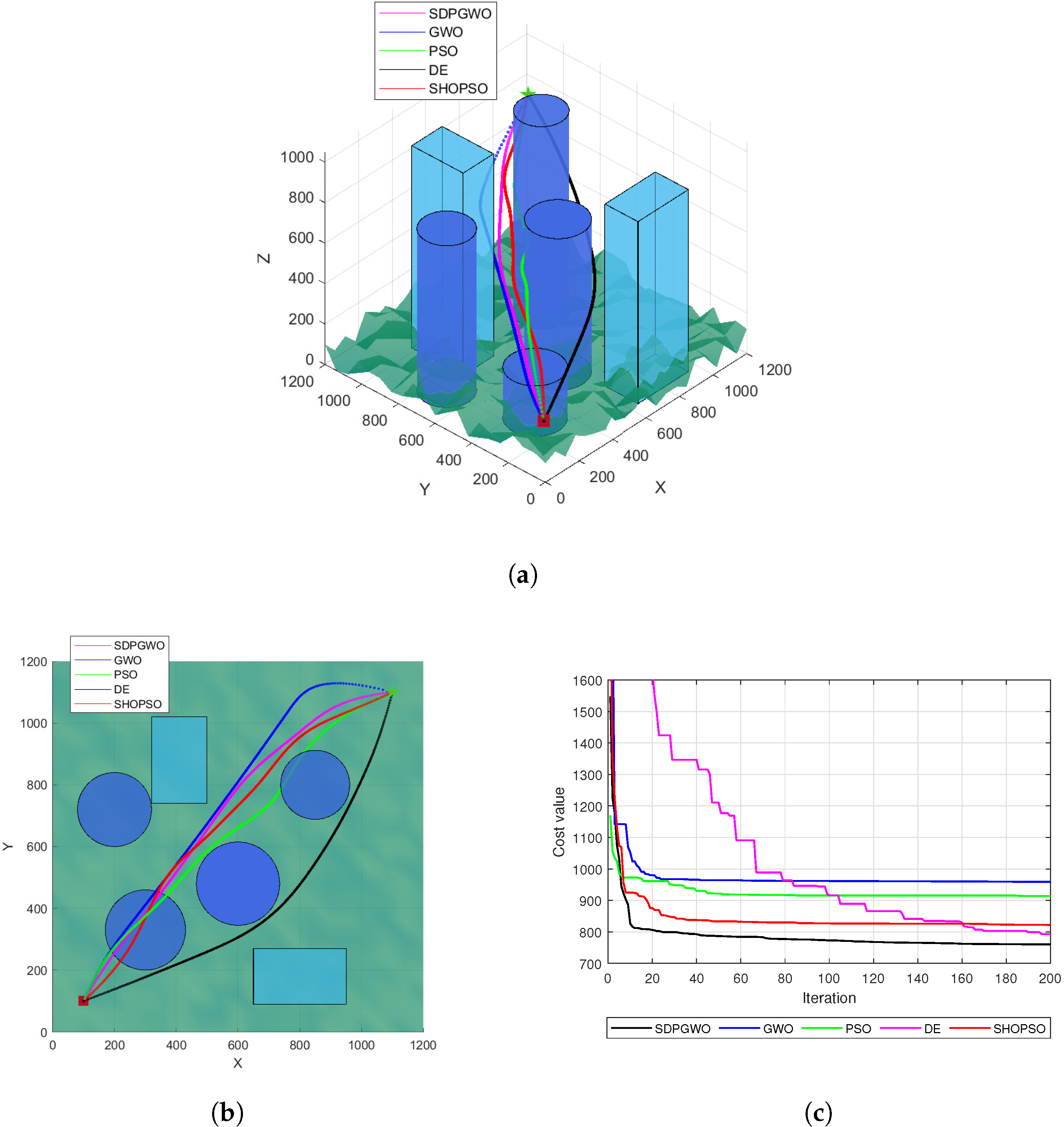
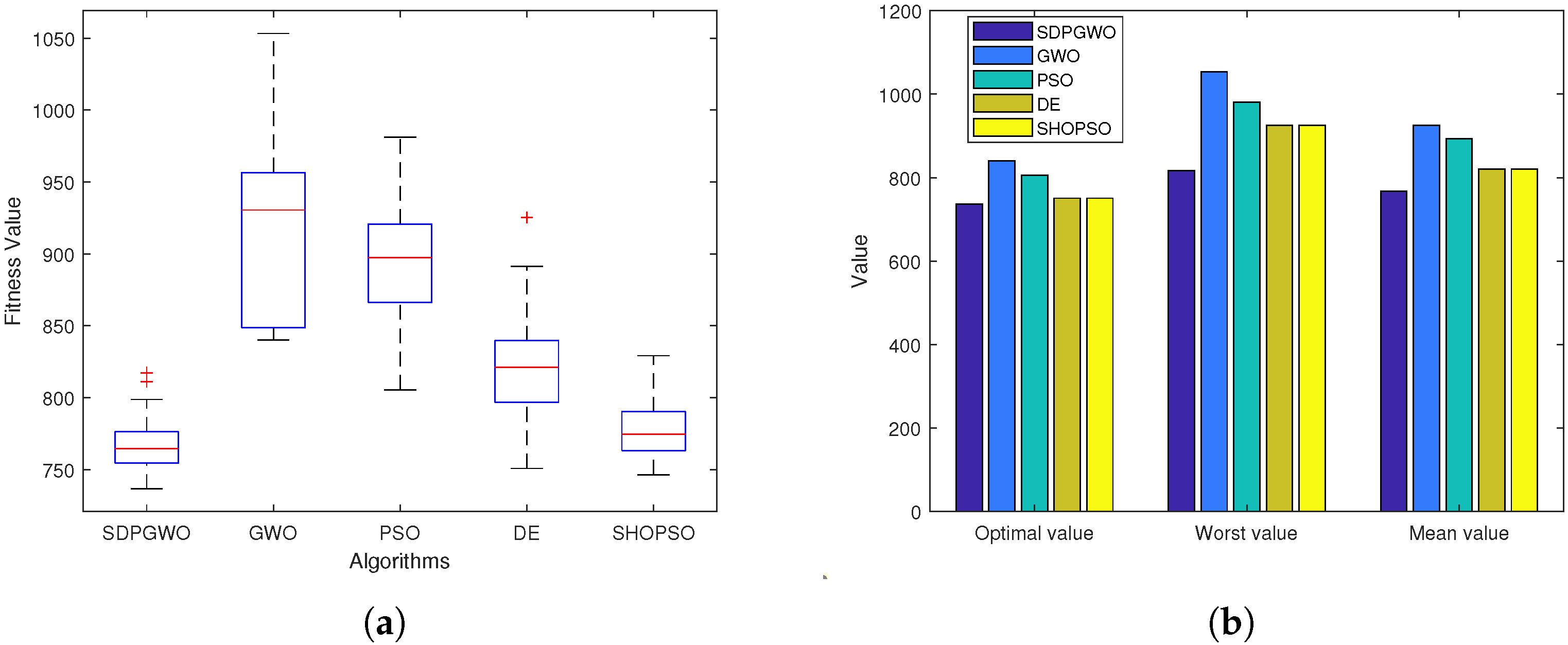
4.2. Experimental Results in Map 2

The performance of the SDPGWO optimizer in 3D path planning was further assessed in a more complex environment (Map 2). In this scenario, eight obstacles were introduced to thoroughly cover the search space, as shown in Table 1. The goal for all optimizers was to find a feasible path from $S(100,100,200)$ to $T(1100,1100,800)$ while avoiding collisions with these obstacles. Due to the increased complexity of Map 2 compared with Map 1, which made the optimization task more challenging, the total number of iterations was set to 300 to ensure sufficient exploration and convergence of the algorithms. The number of waypoints was 10. The other experimental parameters were maintained as outlined in Section 4.1, and all the experiments were executed independently 50 times.

Figure 9a shows the simulated and smoothed paths generated by the five algorithms in the 3D environment for Map 2, while Figure 9b presents the top view. These figures reveal that only the SHOPSO and SDPGWO algorithms managed to avoid collisions with obstacles. However, the path output by SHOPSO was longer compared with that by the SDPGWO algorithm, suggesting that it was not the optimal flight path to the target. The path generated by SDPGWO was more suitable and smoother, highlighting the employability of SDPGWO for path planning. Figure 9c presents the convergence curves for all five algorithms in Map 2. It is evident from the curves that the SDPGWO algorithm reached the optimal value around the 180th iteration. In contrast, other algorithms exhibited slower convergence and weaker optimization abilities, often getting trapped in local minima. This highlights the superior performance and robustness of SDPGWO, particularly in more challenging environments like Map 2.

As demonstrated in

Table 5. Comparison of results after 50 repetitions in Map 2.

NO.	Indicators	SDPGWO	SHOPSO	GWO	PSO	DE
1	Optimal	$5.5361\times {10}^2$	$5.5538\times {10}^2$	$6.5747\times {10}^2$	$6.1185\times {10}^2$	$5.6073\times {10}^2$
2	Worst	$5.6876\times {10}^2$	$6.1192\times {10}^2$	$7.4998\times {10}^2$	$8.0419\times {10}^2$	$7.0157\times {10}^2$
3	Mean	$5.5577\times {10}^2$	$5.7322\times {10}^2$	$7.1737\times {10}^2$	$6.9139\times {10}^2$	$6.1172\times {10}^2$
4	Std	6.9936	12.3943	27.5461	44.0027	32.3388
5	Path length	1612.48	1653.29	1783.50	1773.81	1688.23
6	Runtime (s)	92.36	95.38	74.62	78.27	81.34
7	SR (%)	98.0	90.0	28.0	34.0	62.0

and Figure 10, the SDPGWO algorithm exhibits compelling performance in Map 2. In comparison with the other four algorithms, SDPGWO can achieve more satisfactory results. Specifically, SDPGWO yields the lowest Optimal (553.6), Mean (555.8), and Std (6.99) fitness values, indicating effective and stable optimization. Furthermore, SDPGWO generates the shortest average path length (1612.48) and achieves a high success rate (SR) of 98%. SHOPSO closely follows SDPGWO in overall performance, exhibiting the second-best Optimal and Mean fitness values and a strong SR of 90%. Although SDPGWO’s runtime (92.36s) is slightly longer than that of GWO, PSO, and DE, the difference is not substantial, and is outweighed by its superior path quality and reliability. These data underscore SDPGWO’s robust global optimization capability and overall effectiveness in challenging UAV path planning scenarios.

5. Conclusions

In this research, we tackle the challenge of optimizing UAV flight paths within complex environments. To achieve this objective of finding the shortest viable route for unmanned aerial vehicles, we introduce a novel SDPGWO algorithm. The SDPGWO algorithm improves upon the standard GWO by incorporating two strategies: reducing the computational complexity through a simplification strategy and enhancing global search capability with a differential perturbation strategy. Finally, two simulation examples and comparative results from specific UAV path planning scenarios demonstrate that the SDPGWO algorithm achieves superior performance compared with other methods in efficiently planning high-quality, flyable paths for UAVs.

However, it is important to acknowledge the limitations of the current study. For example, our experimental validation primarily focused on static, three-dimensional environments. Real-world UAV applications are often more complex and may involve dynamic environmental factors and uncertainties. Building upon this work, several promising avenues for future research emerge. First, extending the SDPGWO algorithm to multi-UAV three-dimensional cooperative path planning problems is an important research direction. Second, to cope with increasingly complex task environments, such as larger-scale maps, denser obstacles, and more stringent real-time requirements, seeking more efficient optimization algorithms remains a key direction for future research.

References

1. Skorobogatov, G.; Barrado, C.; Salamí, E. Multiple UAV systems: A survey. Unmanned Syst. 2020, 8, 149–169. [Google Scholar] [CrossRef]
2. Qu, L.D.; Jia, Y.J.; Li, X.Q.; Fan, J.K. Two-stage control model based on enhanced elephant clan optimization for path planning of unmanned combat aerial vehicle. J. Supercomput. 2024, 80, 24938–24974. [Google Scholar] [CrossRef]
3. Erdelj, M.; Natalizio, E.; Chowdhury, K.R.; Akyildiz, I.F. Help from the sky: Leveraging UAVs for disaster management. IEEE Pervas. Comput. 2017, 16, 24–32. [Google Scholar] [CrossRef]
4. Shakhatreh, H.; Sawalmeh, A.H.; Al-Fuqaha, A.; Dou, Z.C.; Almaita, E.; Khalil, I.; Othman, N.S.; Khreishah; Guizani, M. Unmanned aerial vehicles (UAVs): A survey on civil applications and key research challenges. IEEE Access 2019, 7, 48572–48634. [Google Scholar] [CrossRef]
5. Zhen, Z.Y.; Xing, D.J.; Gao, C. Cooperative search-attack mission planning for multi-UAV based on intelligent self-organized algorithm. Aerosp. Sci. Technol. 2018, 76, 402–411. [Google Scholar] [CrossRef]
6. Yang, P.; Tang, K.; Lozano, J.A.; Cao, X.B. Path planning for single unmanned aerial vehicle by separately evolving waypoints. IEEE Trans. Robot. 2015, 31, 1130–1146. [Google Scholar] [CrossRef]
7. Qadir, Z.; Zafar, M.H.; Moosavi, S.K.R.; Le, K.N.; Mahmud, M.A.P. Autonomous UAV path-planning optimization using metaheuristic approach for predisaster assessment. IEEE Internet Things 2021, 9, 12505–12514. [Google Scholar] [CrossRef]
8. Zhang, Z.; Li, J.X.; Wang, J. Sequential convex programming for nonlinear optimal control problems in UAV path planning. Aerosp. Sci. Technol. 2018, 76, 280–290. [Google Scholar] [CrossRef]
9. Dewangan, R.K.; Shukla, A.; Godfrey, W.W. Three dimensional path planning using Grey wolf optimizer for UAVs. Appl. Intell. 2019, 49, 2201–2217. [Google Scholar] [CrossRef]
10. Sun, T.; Sun, W.; Sun, C.; He, R. Multi-UAV Formation Path Planning Based on Compensation Look-Ahead Algorithm. Drones 2024, 8, 251. [Google Scholar] [CrossRef]
11. Wu, Y.; Wu, S.B.; Hu, X.T. Cooperative path planning of UAVs & UGVs for a persistent surveillance task in urban environments. IEEE Internet Things 2020, 8, 4906–4919. [Google Scholar]
12. He, W.J.; Qi, X.G.; Liu, L.F. A novel hybrid particle swarm optimization for multi-UAV cooperate path planning. Appl. Intell. 2021, 51, 7350–7364. [Google Scholar] [CrossRef]
13. Xu, L.; Cao, X.B.; Du, W.B.; Li, Y.M. Cooperative path planning optimization for multiple UAVs with communication constraints. Knowl.-Based Syst. 2023, 260, 110164. [Google Scholar] [CrossRef]
14. Baek, J.; Han, S.I.; Han, Y. Energy-efficient UAV routing for wireless sensor network. IEEE Trans. Veh. Technol. 2019, 69, 1741–1750. [Google Scholar] [CrossRef]
15. Baumann, M.; Léonard, S.; Croft, E.A.; Little, J.J. Path planning for improved visibility using a probabilistic road map. IEEE Trans. Robot. 2010, 26, 195–200. [Google Scholar] [CrossRef]
16. Kothari, M.; Postlethwaite, I. A probabilistically robust path planning algorithm for UAVs using rapidly-exploring random trees. J. Intell. Robot. Syst. 2013, 71, 231–253. [Google Scholar] [CrossRef]
17. Liu, X.H.; Zhang, D.G.; Zhang, T.; Cui, Y.Y.; Chen, L.; Liu, S. Novel best path selection approach based on hybrid improved A* algorithm and reinforcement learning. Appl. Intell. 2021, 51, 9015–9029. [Google Scholar] [CrossRef]
18. Silva Arantes, J.; Silva Arantes, M.; Motta Toledo, C.F.; Trindade Júnior, O.; Williams, B.C. Heuristic and genetic algorithm approaches for UAV path planning under critical situation. Int. J. Artif. Intell. Tools 2017, 26, 1760008. [Google Scholar] [CrossRef]
19. Gao, C.; Zhen, Z.Y.; Gong, H.J. A self-organized search and attack algorithm for multiple unmanned aerial vehicles. Aerosp. Sci. Technol. 2016, 54, 229–240. [Google Scholar] [CrossRef]
20. Shao, S.K.; Peng, Y.; He, C.L.; Du, Y. Efficient path planning for UAV formation via comprehensively improved particle swarm optimization. ISA Trans. 2020, 97, 415–430. [Google Scholar] [CrossRef]
21. Zhang, S.; Zhou, Y.Q.; Li, Z.M.; Pan, W. Grey wolf optimizer for unmanned combat aerial vehicle path planning. Adv. Eng. Softw. 2016, 99, 121–136. [Google Scholar] [CrossRef]
22. Zhang, X.Y.; Duan, H.B. An improved constrained differential evolution algorithm for unmanned aerial vehicle global route planning. Appl. Soft Comput. 2015, 26, 270–284. [Google Scholar] [CrossRef]
23. Zhao, R.X.; Wang, Y.L.; Xiao, G.; Liu, C.; Hu, P.; Li, H. A method of path planning for unmanned aerial vehicle based on the hybrid of selfish herd optimizer and particle swarm optimizer. Appl. Intell. 2022, 52, 16775–16798. [Google Scholar] [CrossRef]
24. Meng, Q.; Chen, K.; Qu, Q. PPSwarm: Multi-UAV Path Planning Based on Hybrid PSO in Complex Scenarios. Drones 2024, 8, 192. [Google Scholar] [CrossRef]
25. Gupta, H.; Verma, O.P. A novel hybrid Coyote-Particle Swarm Optimization Algorithm for three-dimensional constrained trajectory planning of Unmanned Aerial Vehicle. Appl. Soft Comput. 2023, 147, 110776. [Google Scholar] [CrossRef]
26. Yu, Z.H.; Si, Z.J.; Li, X.B.; Wang, D.; Song, H.B. A novel hybrid particle swarm optimization algorithm for path planning of UAVs. IEEE Internet Things 2022, 9, 22547–22558. [Google Scholar] [CrossRef]
27. Qu, C.Z.; Gai, W.D.; Zhang, J.; Zhong, M.Y. A novel hybrid grey wolf optimizer algorithm for unmanned aerial vehicle (UAV) path planning. Knowl.-Based Syst. 2020, 194, 105530. [Google Scholar] [CrossRef]
28. Wang, J.; Wang, W.C.; Hu, X.X.; Qiu, L.; Zang, H.F. Black-winged kite algorithm: A nature-inspired meta-heuristic for solving benchmark functions and engineering problems. Artif. Intell. Rev. 2024, 57, 98. [Google Scholar] [CrossRef]
29. Zhang, Z.; Wang, X.K.; Yue, Y.G. Heuristic optimization algorithm of black-winged kite fused with osprey and its engineering application. Biomimetics 2024, 9, 595. [Google Scholar] [CrossRef]
30. Abbasi, S.; Rahmani, A.M.; Balador, A.; Sahafi, A. A fault-tolerant adaptive genetic algorithm for service scheduling in internet of vehicles. Appl. Soft Comput. 2023, 143, 110413. [Google Scholar] [CrossRef]
31. Fan, J.Y.; Zhou, X. Optimization of a hybrid solar/wind/storage system with bio-generator for a household by emerging metaheuristic optimization algorithm. J. Energy Storage 2023, 73, 108967. [Google Scholar] [CrossRef]
32. Mirjalili, S.; Mirjalili, S.M.; Lewis, A. Grey wolf optimizer. Adv. Eng. Softw. 2014, 69, 46–61. [Google Scholar] [CrossRef]
33. Wang, S.W.; Zhu, D.L.; Zhou, C.J.; Sun, G.J. Improved grey wolf algorithm based on dynamic weight and logistic mapping for safe path planning of UAV low-altitude penetration. J. Supercomput. 2024, 80, 25818–25852. [Google Scholar] [CrossRef]
34. Miao, Z.M.; Yuan, X.F.; Zhou, F.Y.; Qiu, X.J.; Song, Y.; Chen, K. Grey wolf optimizer with an enhanced hierarchy and its application to the wireless sensor network coverage optimization problem. Appl. Soft Comput. 2020, 96, 106602. [Google Scholar] [CrossRef]
35. Yu, X.B.; Wu, X.J. Ensemble grey wolf Optimizer and its application for image segmentation. Expert. Syst. Appl. 2022, 209, 118267. [Google Scholar] [CrossRef]
36. Wang, Z.D.; Dai, D.H.; Zeng, Z.Y.; He, D.J.; Chan, S. Multi-strategy enhanced Grey Wolf Optimizer for global optimization and real world problems. Cluster Comput. 2024, 27, 10671–10715. [Google Scholar] [CrossRef]
37. Tu, Q.; Chen, X.C.; Liu, X.C. Multi-strategy ensemble grey wolf optimizer and its application to feature selection. Appl. Soft Comput. 2019, 76, 16–30. [Google Scholar] [CrossRef]
38. Preeti; Deep, K. A random walk Grey wolf optimizer based on dispersion factor for feature selection on chronic disease prediction. Expert Syst. Appl. 2022, 206, 117864. [Google Scholar] [CrossRef]
39. Dereli, S. A new modified grey wolf optimization algorithm proposal for a fundamental engineering problem in robotics. Neural Comput. Appl. 2021, 33, 14119–14131. [Google Scholar] [CrossRef]
40. Amirsadri, S.; Mousavirad, S.J.; Ebrahimpour-Komleh, H. A Levy flight-based grey wolf optimizer combined with back-propagation algorithm for neural network training. Neural Comput. Appl. 2018, 30, 3707–3720. [Google Scholar] [CrossRef]
41. Zhang, X.M.; Lin, Q.Y.; Mao, W.T.; Liu, S.W.; Dou, Z.; Liu, G.Q. Hybrid Particle Swarm and Grey Wolf Optimizer and its application to clustering optimization. Appl. Soft Comput. 2021, 101, 107061. [Google Scholar] [CrossRef]
42. Tu, B.B.; Wang, F.; Huo, Y.; Wang, X.T. A hybrid algorithm of grey wolf optimizer and harris hawks optimization for solving global optimization problems with improved convergence performance. Sci. Rep. 2023, 13, 22909. [Google Scholar] [CrossRef] [PubMed]
43. Yu, X.B.; Jiang, N.J.; Wang, X.M.; Li, M.Y. A hybrid algorithm based on grey wolf optimizer and differential evolution for UAV path planning. Expert Syst. Appl. 2023, 215, 119327. [Google Scholar] [CrossRef]
44. Qu, C.Z.; Gai, W.D.; Zhong, M.Y.; Zhang, J. A novel reinforcement learning based grey wolf optimizer algorithm for unmanned aerial vehicles (UAVs) path planning. Appl. Soft Comput. 2020, 89, 106099. [Google Scholar] [CrossRef]
45. Jiang, W.; Lyu, Y.X.; Li, Y.F.; Guo, Y.C.; Zhang, W.G. UAV path planning and collision avoidance in 3D environments based on POMPD and improved grey wolf optimizer. Aerosp. Sci. Technol. 2022, 121, 107314. [Google Scholar] [CrossRef]
46. Huo, L.S.; Zhu, J.H.; Li, Z.M.; Ma, M.H. A hybrid differential symbiotic organisms search algorithm for UAV path planning. Sensors 2021, 21, 3037. [Google Scholar] [CrossRef]
47. Ibrahim, R.A.; Abd Elaziz, M.; Lu, S.F. Chaotic opposition-based grey-wolf optimization algorithm based on differential evolution and disruption operator for global optimization. Expert Syst. Appl. 2018, 108, 1–27. [Google Scholar] [CrossRef]
Figure 2. Top view of the UAV path planning model.
Drones 09 00212 g002
Figure 3. Map 1 simulation results when n = 8 . (a) The path planning results in 3D view. (b) Top view of UAV path planning. (c) Convergence curves for the cost function.
Drones 09 00212 g003
Figure 4. Map 1 simulation results when n = 10 . (a) The path planning results in 3D view. (b) Top view of UAV path planning. (c) Convergence curves for the cost function.
Drones 09 00212 g004
Figure 5. Map 1 simulation results when n = 12 . (a) The path planning results in 3D view. (b) Top view of UAV path planning. (c) Convergence curves for the cost function.
Drones 09 00212 g005
Figure 6. Performance comparison of algorithms in Map 1 when n = 8 . (a) Data distribution of four algorithms. (b) Statistical results of four algorithms.
Drones 09 00212 g006
Figure 7. Performance comparison of algorithms in Map 1 when n = 10 . (a) Data distribution of four algorithms. (b) Statistical results of four algorithms.
Drones 09 00212 g007
Figure 8. Performance comparison of algorithms in Map 1 when n = 12 . (a) Data distribution of four algorithms. (b) Statistical results of four algorithms.
Drones 09 00212 g008
Figure 9. Simulation results of UAV path planning in Map 2. (a) The path planning results in 3D view. (b) Top view of UAV path planning. (c) Convergence curves for the cost function.
Drones 09 00212 g009
Figure 10. Performance comparison of algorithms in Map 2. (a) Data distribution of four algorithms. (b) Statistical results of four algorithms.
Drones 09 00212 g010