Preassigned Fixed-Time Synergistic Constrained Control for Fixed-Wing Multi-UAVs with Actuator Faults

Abstract

This study focuses on the distributed fixed-time fault-tolerant control problem for a network of six-degree-of-freedom (DOF) fixed-wing unmanned aerial vehicles (UAVs), which are subject to full-state constraints and actuator faults. The novelty of the proposed design lies in the incorporation of an enhanced asymmetric time-varying tan-type barrier Lyapunov function (BLF), which is applicable in both constrained and unconstrained scenarios. This function ensures that the UAV states remain within compact sets at all times while achieving fixed-time convergence. Additionally, a fixed-time performance function (FTPF) is developed to eliminate the dependency on exponential functions commonly used in traditional fixed-time control methods. The adverse effects of actuator faults, including lock-in-place and loss of effectiveness, are mitigated through a bounded uniform tracking control design. A rigorous Lyapunov function analysis demonstrates that all closed-loop signals are semi-globally uniformly ultimately bounded (SGUUB), with both velocity and attitude tracking errors converging to residual sets near the origin. Experimental validation tests are conducted to confirm the effectiveness of the theoretical findings.

1. Introduction

The coordinated operation of multiple fixed-wing unmanned aerial vehicles (UAVs) has gained significant attention in recent years, primarily because of its benefits in terms of mission performance and cost-effectiveness [1,2,3,4,5]. Research into cooperative control methods has primarily focused on maintaining and adapting formation shapes, as well as synchronizing velocity and attitude in UAV formations. Among these approaches, distributed control strategies have garnered significant attention because they ensure closed-loop stability without relying on global information [1,2]. Building on the existing body of work on distributed cooperative control, several key advancements have been made [6,7,8]. For instance, Qian et al. [6] explored distributed fault-tolerant tracking control and obstacle avoidance for multiple UAVs while addressing lumped disturbances and potential communication failures. Similarly, Yang et al. [7] combined distributed model predictive control with image-based visual servoing to tackle collaborative tracking challenges. Choi et al. [8] proposed a distributed coordinated control method for UAVs with dynamic event-triggered communication. However, the methods in [6,7,8] simplify UAV dynamics to three degrees of freedom or consider only attitude and longitudinal dynamics. In contrast, actual fixed-wing UAVs operate with a nonlinear dynamic model consisting of six-degree-of-freedom (DOF) and twelve state variables, covering both rotational and translational dynamics, necessitating a more comprehensive investigation into six-DOF dynamics [9,10,11]. Zhang et al. [9] developed a dynamic event-triggered communication mechanism to minimize communication load while conserving network resources, and this approach was extended to cooperative path-following for multiple six-DOF UAVs in [10]. Additionally, Lv et al. [11] addressed actuator saturation and failures under the six-DOF model. Nonetheless, the above-mentioned results in [9,10,11] did not take into account state constraints, which are critical for practical applications.

State constraints are essential in practical systems, as their violation can lead to degraded dynamic performance or even system instability [12,13,14,15,16,17,18,19,20,21,22,23,24,25]. Ensuring that system states remain within predefined compact sets is thus vital for safety considerations. Barrier Lyapunov functions (BLFs) have proven to be effective tools for addressing state constraints while ensuring closed-loop stability. Several types of BLFs have been introduced, including log-type [12,13,14], integral-type [15,16,17], and tan-type [18,19,20,21,22,23]. Among these, the tan-type BLF offers advantages over the log-type, as it remains effective even in unconstrained systems. Due to this superiority, tan-type BLFs have been widely explored, with notable results presented in [18,19,20,21,22]. For example, Sun et al. [18] combined tan-type BLFs with backstepping and fuzzy control to manage state constraints in high-order uncertain nonlinear systems, while Tang et al. [20] proposed an event-triggered adaptive fuzzy output feedback control scheme for nonlinear switched systems with full state constraints. However, these studies focus on strict-feedback systems, which are not directly applicable to fixed-wing UAVs, and current tan-type BLFs are symmetric and designed for infinite-time convergence, not fixed-time.

It needs to be emphasized that lots of practical applications have a high requirement for strict time response constraints and how to guarantee the convergence time is a worthwhile topic in the operation process of actual systems. Recently, finite/fixed-time control methods have emerged as key tools to address this challenge [26,27,28,29,30]. However, finite-time controllers have a drawback in that convergence time depends on initial conditions and is not explicitly defined [26]. In contrast, fixed-time controllers define an upper bound for convergence time that is independent of initial conditions. Based on this, a significant body of research has been developed [27,28,29,30]. Zhang et al. [27] introduced a fixed-time stabilization method for nonlinear systems, emphasizing dynamic parameter design to ensure global stability within a fixed time. Sui et al. [28] developed a nonsingular fixed-time adaptive tracking control scheme for multiple-input multiple-output nonlinear systems with a nonstrict feedback structure, using fuzzy logic to identify unknown dynamics and combining adaptive backstepping and power integration to ensure asymptotic error convergence. Unfortunately, these methods often require the agent dynamics to be structured as strict-feedback systems. Furthermore, although traditional fixed-time control (FTC) systems can operate independently of initial system conditions, the convergence time is contingent upon the exponential terms stipulated in the Fixed-Time Stability Theorem (see Remark 3 for more details). Moreover, due to the involvement of numerous uncertain variables in determining a precise fixed time, obtaining an exact solution is notably challenging.

• To better align with practical scenarios, this study develops a distributed cooperative control scheme for multiple UAVs based on a more realistic six-DOF dynamic model. Additionally, a fault-tolerant mechanism is incorporated to address potential actuator failures that may occur during actual flight operations.
• In order to enforce full-state constraints on the UAV system, an improved segmented asymmetric tan-type BLF is introduced. This modification allows for the imposition of asymmetric constraints on the UAV system, which operates as a non-strict feedback system.
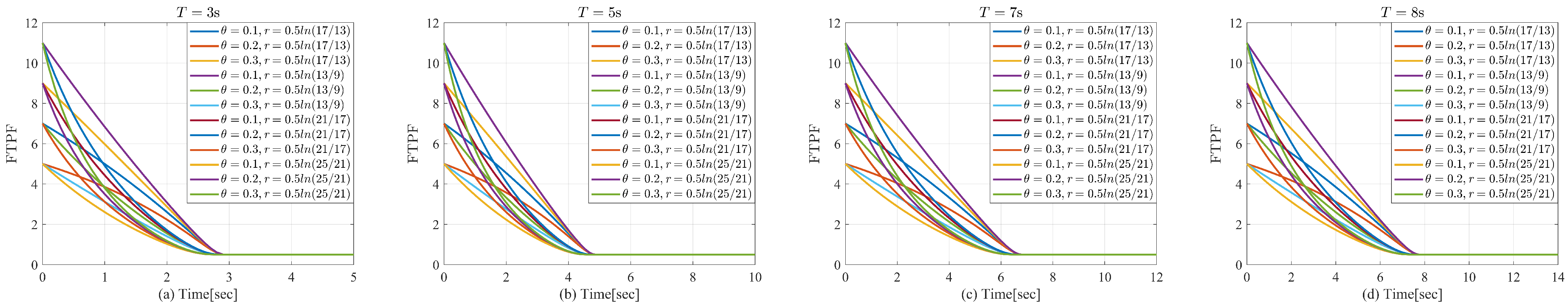
• To achieve fixed-time control for the multi-UAV system under full-state constraints, a novel fixed-time performance function (FTPF) is proposed. When combined with the improved segmented asymmetric tan-BLF, this approach overcomes the limitations of traditional fixed-time convergence methods, which are generally restricted to strict-feedback systems and impose rigid convergence conditions.

Notations.

${\mathbb{R}}^m$ and ${\mathbb{R}}^{m\times n}$ denote the real m-vector and real $m\times n$ matrices, respectively. $∥·∥$ is the Euclidean norm of a vector, ${\lambda }_{min}\left(\mathit{D}\right)$ and ${\lambda }_{max}\left(\mathit{D}\right)$ are the minimum and maximum eigenvalues of the matrix $\mathit{D}$, respectively, $\mathrm{SO}=\left\{\mathcal{R}\in {\mathbb{R}}^{3\times 3}:{\mathcal{R}}^{\mathrm{T}}\mathcal{R}=I_3,\right.$$\left.\det \left(\mathcal{R}\right)=1\right\}$ represents the third-order special orthogonal group. The notation $\mathrm{sig}\left(\mathit{A}\right)$ typically refers to the spectral norm of a diagonal matrix $\mathit{A}$, calculated as the square root of the eigenvalues of ${\mathit{A}}^{\mathrm{T}}\mathit{A}$.

The rest of the article is structured as follows: In Section 2, the dynamic model of UAV, graph theory, neural networks, and the control objectives are introduced. Section 3 discusses the process and stability proof of the adaptive fixed-time controller. In Section 4, the simulation results and their validation are presented. Finally, Section 5 provides the conclusions drawn from the study.

2. Problem Formulation and Preliminaries

2.1. UAV Kinematics and Dynamics

Consider a formation consisting of N 6-DOF fixed-wing UAVs sharing the same dynamic model. According to the Newton–Euler convention, the dynamic model for each UAV can be expressed as follows [9,10,11],

$$\begin{array}{cc}\hfill {\dot{\mathit{I}}}_i=& {\mathcal{R}}_1\left({\mathit{\phi }}_i\right){\mathit{v}}_i\hfill \end{array}$$

(1)

$$\begin{array}{cc}\hfill {\dot{\mathit{v}}}_i=& -\mathcal{X}\left({\mathit{\omega }}_i\right){\mathit{v}}_i+{\displaystyle \frac{{\mathcal{P}}_i}{m_i}}+{\mathcal{R}}_1^{\mathrm{T}}\left({\mathit{\phi }}_i\right)\mathit{g}+{\displaystyle \frac{{\mathcal{F}}_i}{m_i}}+{\mathcal{D}}_{vi}\hfill \end{array}$$

(2)

$$\begin{array}{cc}\hfill {\dot{\mathit{\phi }}}_i=& {\mathcal{R}}_2^{-1}\left({\mathit{\phi }}_i\right){\mathit{\omega }}_i\hfill \end{array}$$

(3)

$$\begin{array}{cc}\hfill {\mathcal{L}}_i{\dot{\mathit{\omega }}}_i=& -\mathcal{X}\left({\mathit{\omega }}_i\right){\mathcal{L}}_i{\mathit{\omega }}_i+{\mathcal{Z}}_i+\mathcal{C}\left({\mathit{\delta }}_i\right){\mathit{\delta }}_i+{\mathcal{L}}_i{\mathcal{D}}_{\omega i}\hfill \end{array}$$

(4)

where ${\mathit{I}}_i={[x_i,y_i,z_i]}^T$ represents the position relative to an inertial frame, ${\mathit{v}}_i={[u_i,v_i,w_i]}^T$ is the linear velocity, ${\mathit{\phi }}_i={[{\varphi }_i,{\theta }_i,{\psi }_i]}^T$ represents the angles of attitude, and ${\mathit{\omega }}_i={[p_i,q_i,r_i]}^T$ represents the angular velocity. Additionally, the thrust vector along the x-axis of the body frame is denoted by ${\mathcal{P}}_i={[P_{xi},0,0]}^T$, while ${\mathit{\delta }}_i={[{\delta }_{ai},{\delta }_{ei},{\delta }_{ri}]}^T$ represents the control input quantity. To facilitate the derivation, the cross product of matrices ${\mathit{\omega }}_i\times {\mathit{v}}_i$ is denoted as $\mathcal{X}\left({\mathit{\omega }}_i\right){\mathit{v}}_i$, and the cross product of matrices ${\mathit{\omega }}_i\times \mathcal{L}{\mathit{\omega }}_i$ is denoted as $\mathcal{X}\left({\mathit{\omega }}_i\right){\mathcal{L}}_i{\mathit{\omega }}_i$. In this context, ${\delta }_{ei},{\delta }_{ai},{\delta }_{ri}$ represent the deflections of the elevator, ailerons, and rudder, respectively. The gravity acceleration is given by $\mathit{g}={[0,0,g_z]}^T$, and the external disturbances are represented by ${\mathcal{D}}_{v_i}\in {\mathbb{R}}^3$ and ${\mathcal{D}}_{\omega i}\in {\mathbb{R}}^3$. The inertia tensor ${\mathcal{L}}_i$ is expressed as

$$\begin{array}{c}\hfill {\mathcal{L}}_i=\left[\begin{array}{ccc}{\mathcal{L}}_{xxi}& 0& {\mathcal{L}}_{xzi}\\ 0& {\mathcal{L}}_{yyi}& 0\\ {\mathcal{L}}_{zxi}& 0& {\mathcal{L}}_{zzi}\end{array}\right]\end{array}$$

(5)

Additionally, the matrix ${\mathcal{R}}_1\left({\mathit{\phi }}_i\right)\in \mathrm{SO}\left(3\right)$ is responsible for transforming coordinates from the body frame to the inertial frame. Meanwhile, the matrix ${\mathcal{R}}_2\left({\mathit{\phi }}_i\right)\in {\mathbb{R}}^{3\times 3}$ is used to convert the time derivative of the Euler angles into the non-inertial representation of angular velocity. The following provides the expressions for these matrices:

$$\begin{array}{cc}\hfill {\mathcal{R}}_1\left({\mathit{\phi }}_i\right)=& \left[\begin{array}{c}{C}_{\psi i}{C}_{\theta i}-S_{\psi i}{S}_{\varphi i}+C_{\psi i}{S}_{\theta i}{S}_{\varphi i}{S}_{\psi i}{s}_{\varphi i}+C_{\psi i}{S}_{\theta i}{C}_{\varphi i}\hfill \\ S_{\psi i}{C}_{\theta i}{C}_{\psi i}{C}_{\varphi i}+S_{\psi i}{S}_{\theta i}{S}_{\varphi i}-C_{\psi i}{S}_{\varphi i}+S_{\psi i}{S}_{\theta i}{C}_{\varphi i}\hfill \\ -S_{\theta i}{C}_{\theta i}{S}_{\varphi i}{C}_{\theta i}{C}_{\varphi i}\hfill \end{array}\right]\hfill \\ \hfill {\mathcal{R}}_2\left({\mathit{\phi }}_i\right)=& \left[\begin{array}{ccc}1& 0& -S_{\psi i}\\ 0& C_{\psi i}& S_{\psi i}{C}_{\theta i}\\ 0& -S_{\theta i}& C_{\psi i}{C}_{\theta i}\end{array}\right]\hfill \end{array}$$

(6)

where $S_a$ and $C_a$ represent $sin\left(a\right)$ and $cos\left(a\right)$, respectively. The aerodynamic forces, expressed as ${\mathcal{F}}_i={[F_{Xi},F_{Yi},F_{Zi}]}^T$, and the moments, given by ${\mathcal{Z}}_i={[F_{Li},F_{Mi},F_{Ni}]}^T$, are determined using aerodynamic coefficients.

$$\begin{array}{cc}\hfill {\mathcal{F}}_i=& {\overline{q}}_i{S}_i{\mathcal{R}}_3^{-1}\left({\alpha }_i,{\beta }_i\right){\left[-K_{Di},K_{Yi},-K_{Li}\right]}^{\mathrm{T}}\hfill \end{array}$$

(7)

$$\begin{array}{cc}\hfill {\mathcal{Z}}_i=& {\overline{q}}_i{S}_i{\left[b_i{K}_{li}^{\prime },{\overline{c}}_i{K}_{Mi}^{\prime },b_i{K}_{ni}^{\prime }\right]}^{\mathrm{T}}\hfill \end{array}$$

(8)

where ${\overline{q}}_i={\displaystyle \frac{1}{2}}\rho V_i^2$ is the dynamic pressure, ${\alpha }_i$ is the angle of attack, and ${\beta }_i$ is the sideslip angle. In addition, the air density $\rho$, wingspan $B_i$, wing surface area $S_i$, and mean aerodynamic chord ${\overline{c}}_i$ are considered constant values. The transformation matrix ${\mathcal{R}}_3({\alpha }_i,{\beta }_i)$ is defined as follows:

$$\begin{array}{c}\hfill {\mathcal{R}}_3\left({\alpha }_i,{\beta }_i\right)=\left[\begin{array}{ccc}{C}_{\alpha i}{C}_{\beta i}& S_{\beta i}& S_{\alpha i}{C}_{\beta i}\\ -C_{\alpha i}{S}_{\beta i}& C_{\beta i}& -S_{\alpha i}{S}_{\beta i}\\ -S_{\alpha i}& 0& C_{\alpha i}\end{array}\right]\end{array}$$

(9)

Finally, the dimensionless aerodynamic coefficients $K_{Di}$, $K_{Yi}$, $K_{Li}$, $K_{li}^{\prime }$, $K_{Mi}^{\prime }$, $K_{ni}^{\prime }$ are defined in the force/moment expressions. Detailed descriptions of these coefficients are provided in [31]. The matrix representing control effectiveness is expressed as

$$\begin{array}{c}\hfill \mathcal{C}\left({\mathit{\delta }}_i\right)=\left[\begin{array}{ccc}{\overline{q}}_i{S}_i{B}_i{C}_{l\delta ai}& 0& {\overline{q}}_i{S}_i{B}_i{C}_{l\delta ri}\\ 0& {\overline{q}}_i{S}_i{\overline{C}}_i{c}_{m\delta ei}& 0\\ {\overline{q}}_i{S}_i{B}_i{C}_{n\delta ai}& 0& {\overline{q}}_i{S}_i{B}_i{C}_{n\delta ri}\end{array}\right]\end{array}$$

(10)

2.2. A Control-Based Model Incorporating Actuator Failures and Modeling Uncertainties

As stated in [9,10,11], the system can be categorized into two interconnected subsystems: translational kinematics, described by Equations (1) and (2), and rotational kinematics, governed by Equations (3) and (4).

2.2.1. Translational Kinematics

From (2), the resultant velocity and its time derivative are given by

$$\begin{array}{c}\hfill {\dot{V}}_i={\displaystyle \frac{{\mathit{v}}_i^{\mathrm{T}}{\dot{\mathit{v}}}_i}{V_i}}={\displaystyle \frac{{\mathit{v}}_i^{\mathrm{T}}}{V_i}}\left(-\mathcal{X}\left({\mathit{\omega }}_i\right){\mathit{v}}_i+{\displaystyle \frac{{\mathcal{P}}_i}{m_i}}+{\mathcal{R}}_1^{\mathrm{T}}\left({\mathit{\phi }}_i\right)\mathit{g}+{\displaystyle \frac{{\mathcal{F}}_i}{m_i}}+{\mathcal{D}}_{vi}\right)\end{array}$$

(11)

where $V_i$ is the velocity vector and $v_i$ corresponds to the scalar velocity, satisfying $V_i=∥v_i∥=\sqrt{v_i^T{v}_i}$.

Using (11) and the definition ${\mathcal{P}}_i={[P_{xi},0,0]}^{\mathrm{T}}$ along with the property ${\mathit{v}}_i^{\mathrm{T}}\mathcal{X}\left({\mathit{\omega }}_i\right){\mathit{v}}_i=0$, we obtain

$$\begin{array}{c}\hfill {\dot{V}}_i={\displaystyle \frac{u_i{P}_{xi}}{m_i{V}_i}}+{\displaystyle \frac{{\mathit{v}}_i^{\mathrm{T}}}{V_i}}\left({\mathcal{R}}_1^{\mathrm{T}}\left({\mathit{\phi }}_i\right)\mathit{g}+{\displaystyle \frac{{\mathcal{F}}_i}{m_i}}+{\mathcal{D}}_{vi}\right)\end{array}$$

(12)

During flight, unknown faults in thrust can be modeled as

$$\begin{array}{c}\hfill P_{xi}={\ell }_{Pi}{P}_{xi0}+P_{xif}\end{array}$$

(13)

where $P_{xi0}$ represents the nominal control input, $0\le {\ell }_{Pi}\le 1$ is the thrust drive efficiency, and $P_{xif}$ is an additional bounded fault. And (13) implies four possible cases:

• ${\ell }_{Pi}=1$ and $P_{xif}=0$. The system is fault-free.
• $0<{\ell }_{Pi}<1$ and $P_{xif}=0$. This represents a partial failure.
• ${\ell }_{Pi}=1$ and $P_{xif}\ne 0$. A bias fault is present.
• ${\ell }_{Pi}=0$ and $P_{xif}\ne 0$. A complete malfunction with a bias fault.

Considering uncertainties in aerodynamic coefficients, direct measurement is often difficult, allowing only the values within ${\mathcal{F}}_i$ to be used in controller design. Thus, ${\mathcal{F}}_i$ is decomposed into a known component ${\mathcal{F}}_{i0}$ and an uncertain component $\Delta {\mathcal{F}}_i$ [9]. Consequently, the translational kinematics is reformulated as

$$\begin{array}{cc}\hfill {\dot{V}}_i=& {\displaystyle \frac{u_i{\rho }_{Pi}{P}_{xi0}}{m_i{V}_i}}+{\displaystyle \frac{u_i{P}_{xif}}{m_i{V}_i}}+{\displaystyle \frac{{\mathit{v}}_i^{\mathrm{T}}}{V_i}}\left({\mathcal{R}}_1^{\mathrm{T}}\left({\mathit{\phi }}_i\right)\mathit{g}+{\displaystyle \frac{{\mathcal{F}}_{i0}}{m_i}}+{\displaystyle \frac{\Delta {\mathcal{F}}_i}{m_i}}+{\mathcal{D}}_{vi}\right)\hfill \end{array}$$

(14)

2.2.2. Rotational Kinematics

Derived from Equations (3) and (4), the attitude dynamics within the inertial reference frame are represented by the following expression:

$$\begin{array}{cc}\hfill {\dot{\mathit{\phi }}}_i=& {\mathcal{R}}_2^{-1}\left({\mathit{\phi }}_i\right){\mathit{\omega }}_i\hfill \end{array}$$

(15)

$$\begin{array}{cc}\hfill {\dot{\mathit{\omega }}}_i=& {\mathcal{L}}_i^{-1}\mathcal{X}\left({\mathcal{L}}_i{\mathit{\omega }}_i\right){\mathit{\omega }}_i+{\mathcal{L}}_i^{-1}{\mathcal{Z}}_i+{\mathcal{L}}_i^{-1}\mathcal{C}\left({\mathit{\delta }}_i\right){\mathit{\delta }}_i+{\mathcal{D}}_{\omega i}\hfill \end{array}$$

(16)

During flight, the control surfaces can experience general faults, modeled as

$$\begin{array}{c}\hfill {\delta }_{ji}={\ell }_{\delta ji}{\delta }_{ji0}+{\delta }_{jif}\end{array}$$

(17)

where ${\delta }_{ji0}$ is the applied control input for the j-th surface (with $j\in \{a,e,r\}$), $0\le {\ell }_{\delta ji}\le 1$ is the actuator efficiency factor, and ${\delta }_{jif}$ is a stuck or bias fault. And (17) follows similar fault cases as (13).

• ${\ell }_{{\delta }_{ji}}=1$ and ${\delta }_{jif}=0$. The system is fault-free.
• $0<{\ell }_{{\delta }_{ji}}<1$ and ${\delta }_{jif}=0$. This represents a partial failure.
• ${\ell }_{{\delta }_{ji}}=1$ and ${\delta }_{jif}\ne 0$. A bias fault is present.
• ${\ell }_{{\delta }_{ji}}=0$ and ${\delta }_{jif}\ne 0$. A complete malfunction with a bias fault.

To simplify, the actuator fault model is reformulated as

$$\begin{array}{c}\hfill {\mathit{\delta }}_i={\ell }_{\delta i}{\mathit{\delta }}_{i0}+{\mathit{\delta }}_{if},\end{array}$$

(18)

where ${\mathit{\delta }}_{i0}={[{\delta }_{ai0},{\delta }_{ei0},{\delta }_{ri0}]}^{\mathrm{T}},{\ell }_{\delta i}=\mathrm{diag}\{{\ell }_{\delta ai},{\ell }_{\delta ei},{\ell }_{\delta ri}\}$, and ${\mathit{\delta }}_{if}={[{\delta }_{aif},{\delta }_{eif},{\delta }_{rif}]}^{\mathrm{T}}$ represent the control input, fault gain, and bias fault, respectively [5]. When actuator faults are present, the dynamics of angular velocity are redefined as follows:

$$\begin{array}{c}\hfill {\dot{\mathit{\omega }}}_i={\mathcal{L}}_{i0}^{-1}\mathcal{X}\left({\mathcal{L}}_{i0}{\mathit{\omega }}_i\right){\mathit{\omega }}_i+{\mathcal{L}}_{i0}^{-1}{\mathcal{Z}}_{i0}+{\mathcal{L}}_{i0}^{-1}{\mathcal{C}}_0\left({\mathit{\delta }}_i\right){\ell }_{\delta i}{\mathit{\delta }}_{i0}+{\mathit{\zeta }}_{\omega i}+{\mathcal{D}}_{\omega i}\end{array}$$

(19)

where ${\mathit{\zeta }}_{\omega i}=\Delta {\mathcal{L}}_i^{-1}\mathcal{X}\left({\mathcal{L}}_i{\mathit{\omega }}_i\right){\mathit{\omega }}_i+\Delta {\mathcal{L}}_i^{-1}{\mathcal{Z}}_{i0}+\Delta {\mathcal{L}}_i^{-1}\mathcal{C}\left({\mathit{\delta }}_i\right){\ell }_{\mathit{\delta }i}{\mathit{\delta }}_{i0}+\Delta {\mathcal{L}}_{i0}^{-1}{\mathcal{C}}_0\left({\mathit{\delta }}_i\right){\mathit{\delta }}_{if}$ is the aggregated uncertainty caused by actuator failure and modeling uncertainty.

Assumption 1

([9]). Parameter uncertainty terms ${\mathit{\zeta }}_{\omega i}$ and $\Delta {\mathcal{L}}_i^{-1}\mathcal{C}$, as well as the fault parameter matrix ${\ell }_{\delta i}$, are present and satisfy the conditions $∥\Delta {\mathcal{L}}_i^{-1}\mathcal{C}\left({\mathit{\delta }}_i\right){\ell }_{\delta i}({\mathcal{L}}_{i0}^{-1}$${{\mathcal{C}}_0\left({\mathit{\delta }}_i\right){\ell }_{\delta i}{)}^{-1}∥}_{\infty }<1$ and $\partial {\mathit{\zeta }}_{\omega i}/\phantom{\partial {\mathit{\zeta }}_{\omega i}\partial {\mathit{\delta }}_{i0}}\partial {\mathit{\delta }}_{i0}+{\mathcal{L}}_{i0}^{-1}{\mathcal{C}}_0\left({\mathit{\delta }}_i\right){\ell }_{\delta i}\ne 0$.

Assumption 2

([10]). There exists a constant $g_{i,min}$ such that ${\lambda }_{min}\left({\mathcal{L}}_{i0}^{-1}{\mathcal{C}}_0\left({\mathit{\delta }}_i\right)\right)\ge g_{i,min}>0$ where ${\lambda }_{min}(·)$ represents the minimum eigenvalue.

Since ${\mathit{\zeta }}_{\omega i}$ involves the control signal ${\mathit{\delta }}_{i0}$, the use of neural networks to approximate ${\mathit{\zeta }}_{\omega i}$ introduces algebraic loops. To resolve this problem, a low-pass filter method can be utilized to process ${\mathit{\delta }}_{i0}$ [32]. Consequently, ${\mathit{\zeta }}_{\omega i}={\mathit{\zeta }}_{\omega i}^{\prime }+{\mathit{\xi }}_{\omega i}$, where ${\mathit{\xi }}_{\omega i}\in {\mathbb{R}}^3$ represents the filtering error. At this stage, the angular velocity kinematics can be expressed as

$$\begin{array}{c}\hfill {\dot{\mathit{\omega }}}_i={\mathcal{L}}_{i0}^{-1}\mathcal{X}\left({\mathcal{L}}_{i0}{\mathit{\omega }}_i\right){\mathit{\omega }}_i+{\mathcal{L}}_{i0}^{-1}{\mathcal{Z}}_{i0}+{\mathcal{L}}_{i0}^{-1}{\mathcal{C}}_0\left({\mathit{\delta }}_i\right){\ell }_{\delta i}{\mathit{\delta }}_{i0}+{{\mathit{\zeta }}^{\prime }}_{\omega i}+{\mathit{\xi }}_{\omega i}+{\mathcal{D}}_{\omega i}\end{array}$$

(20)

Remark 1.

Assumptions 1 and 2 ensure the controllability of the angular velocity dynamics (19). This suggests that, despite the potential actuator failures as outlined in (19) and the presence of model uncertainties in each UAV, ${\delta }_{i0}$ maintains sufficient control authority, thereby enabling the implementation of fault-tolerant control. It is worth noting that $g_{i,min}$ is used exclusively for analysis purposes and is not required a prior.

2.3. Graph Theory

Let $\mathcal{H}=(\mathcal{N},\mathcal{L},\mathbf{A})$ denote an undirected graph that represents the interaction topology among UAVs. In this graph, $\mathcal{N}=\{n_1,n_2,\cdots ,n_m\}$ denotes the set of UAVs, while $\mathcal{L}\subseteq \mathcal{N}\times \mathcal{N}$ represents the set of links (edges), with each link $(n_i,n_j)$ connecting two nodes. The adjacency matrix $\mathbf{A}=\left[a_{ij}\right]\in {\mathbb{R}}^{m\times m}$ is defined such that $a_{ij}=a_{ji}=1$ when nodes $n_i$ and $n_j$ are connected, and $a_{ij}=a_{ji}=0$ otherwise. Self-loops are excluded so $a_{ii}=0$ for all i.

The weighted degree of a node $n_i$, denoted by ${\delta }_i$, is defined as the sum of the weights of the edges connected to $n_i$, expressed as ${\delta }_i={\sum }_{j=1}^m{a}_{ij}{w}_{ij}$, where $w_{ij}$ is the weight of the edge between $n_i$ and $n_j$. The degree matrix $\mathbf{\Delta }$ is then given as a diagonal matrix with entries ${\delta }_1,{\delta }_2,\cdots ,{\delta }_m$ along its diagonal, resulting in $\mathbf{\Delta }=\mathrm{diag}({\delta }_1,{\delta }_2,\cdots ,{\delta }_m)$. The graph Laplacian matrix is defined by $\Lambda =\mathbf{\Delta }-\mathbf{A}$. The set of neighbors of node $n_i$, denoted by ${\mathcal{M}}_i$, includes all nodes $n_j$ such that $(n_i,n_j)\in \mathcal{L}$.

For leader-following control problems, the graph is extended by introducing a leader node $n_0$. The augmented graph ${\mathcal{H}}^{\prime }=({\mathcal{N}}^{\prime },{\mathcal{L}}^{\prime },{\mathbf{A}}^{\prime })$ is defined where ${\mathcal{N}}^{\prime }=\mathcal{N}\cup \left\{n_0\right\}$. The leader’s influence on the follower nodes is modeled by the leader adjacency matrix $\mathit{C}=\mathrm{diag}(c_1,c_2,\cdots ,c_m)$, where $c_i>0$ indicates that follower i is influenced by the leader, while $c_i=0$ otherwise.

Assumption 3.

The multi-agent system is represented using a connected, undirected graph, where at least one follower node is influenced by the leader node.

Lemma 1

([33]). Consider a connected, undirected graph $\mathit{H}$ with Laplacian matrix Λ. If there exists at least one $c_i>0$, the augmented Laplacian matrix $\mathbf{\Lambda }+\mathbf{C}$ is guaranteed to be positive definite.

2.4. Neural Network Approximation

In this article, radial basis function neural networks (RBF NNs) are employed as a general approximation method to compensate for modeling uncertainties [32,34,35,36]. Let ${\mathbf{\Omega }}_{vi}={\left[{\mathit{v}}_i^{\mathrm{T}},{\mathit{\phi }}_i^{\mathrm{T}},{\mathit{\omega }}_i^{\mathrm{T}},{\mathit{\delta }}_{i0}^{\mathrm{T}}\right]}^{\mathrm{T}}\in {\mathbb{R}}^{12}$ and ${\mathbf{\Omega }}_{\omega i}={\left[{\mathit{v}}_i^{\mathrm{T}},{\mathit{\phi }}_i^{\mathrm{T}},{\mathit{\omega }}_i^{\mathrm{T}},{\mathit{\delta }}_{i0}^{\mathrm{T}}\right]}^{\mathrm{T}}\in {\mathbb{R}}^{12}$. For the unknown continuous functions ${\mathit{\zeta }}_{vi}\left({\mathbf{\Omega }}_{vi}\right)={[{\zeta }_{vi1},{\zeta }_{vi2},{\zeta }_{vi3}]}^{\mathrm{T}}$ and ${\mathit{\zeta }}_{\omega i}^{\prime }\left({\mathbf{\Omega }}_{\omega i}\right)={[{\zeta }_{\omega i1}^{\prime },{\zeta }_{\omega i2}^{\prime },{\zeta }_{\omega i3}^{\prime }]}^{\mathrm{T}}$, RBF NNs can be constructed such that

$$\begin{array}{cc}\hfill {\mathit{\zeta }}_{vij}\left({\mathbf{\Omega }}_{vi}\right)& ={\mathit{J}}_{vij}^{*\mathrm{T}}{\mathit{S}}_{vij}\left({\mathbf{\Omega }}_{vi}\right)+{\mathcal{O}}_{vij}\left({\mathbf{\Omega }}_{vi}\right)\hfill \\ \hfill {\mathit{\zeta }}_{\omega ij}^{\prime }\left({\mathbf{\Omega }}_{\omega i}\right)& ={\mathit{J}}_{\omega ij}^{*\mathrm{T}}{\mathit{S}}_{\omega ij}\left({\mathbf{\Omega }}_{\omega i}\right)+{\mathcal{O}}_{\omega ij}\left({\mathbf{\Omega }}_{\omega i}\right)\hfill \end{array}$$

(21)

where $j=1,2,3$, $o_{vij}\left({\mathbf{\Omega }}_{vi}\right)\in \mathbb{R}$ and $o_{\omega ij}\left({\mathbf{\Omega }}_{\omega i}\right)\in \mathbb{R}$ represent the bounded approximation errors. The idealized weight matrices, ${\mathit{J}}_{vij}^{*\mathrm{T}}\in {\mathbb{R}}^{N\times 1}$ and ${\mathit{J}}_{\omega ij}^{*\mathrm{T}}\in {\mathbb{R}}^{N\times 1}$, correspond to systems with N nodes. ${\mathit{S}}_{vij}\left({\mathbf{\Omega }}_{vi}\right)\in {[S_{vij}^1\left({\mathbf{\Omega }}_{vi}\right),...,S_{vij}^N\left({\mathbf{\Omega }}_{vi}\right)]}^T\in {\mathbb{R}}^N$ and ${\mathit{S}}_{\omega ij}\left({\mathbf{\Omega }}_{\omega i}\right)\in {[S_{\omega ij}^1\left({\mathbf{\Omega }}_{\omega i}\right),...,S_{\omega ij}^N\left({\mathbf{\Omega }}_{\omega i}\right)]}^T\in {\mathbb{R}}^N$ are known vectors consisted Gaussian basis functions $S_{vij}^m\left({\mathbf{\Omega }}_{vi}\right)$ and $S_{\omega ij}^m\left({\mathbf{\Omega }}_{\omega i}\right)$, $m=1,...,N$, commonly selected as the following exponential form:

$$\begin{array}{cc}\hfill S_{vij}^m\left({\mathbf{\Omega }}_{vi}\right)& =exp\left[-{\displaystyle \frac{{\left({\mathbf{\Omega }}_{vi}-{\mathit{\iota }}_{vi}\right)}^{\mathrm{T}}\left({\mathbf{\Omega }}_{vi}-{\mathit{\iota }}_{vi}\right)}{{\kappa }_{vi}^2}}\right]\hfill \\ \hfill S_{\omega ij}^m\left({\mathbf{\Omega }}_{\omega i}\right)& =exp\left[-{\displaystyle \frac{{\left({\mathbf{\Omega }}_{\omega i}-{\mathit{\iota }}_{\omega i}\right)}^{\mathrm{T}}\left({\mathbf{\Omega }}_{\omega i}-{\mathit{\iota }}_{\omega i}\right)}{{\kappa }_{\omega i}^2}}\right]\hfill \end{array}$$

(22)

where ${\mathit{\iota }}_{vi}\in {\mathbb{R}}^{12}$ and ${\mathit{\iota }}_{\omega i}\in {\mathbb{R}}^{12}$ denote the centers of the receptive field, while ${\kappa }_{vi}$ and ${\kappa }_{\omega i}$ correspond to the widths of the Gaussian basis functions.

2.5. Control Objective

Considering the presence of actuator faults, modeling uncertainties, and external disturbances, and taking into account the multi-UAV undirected graph topology with a leader, the desired tracking commands, $V_r$ and ${\phi }_r$, are assigned to each UAV. The objective is to design a distributed time-tracking controller to achieve the following:

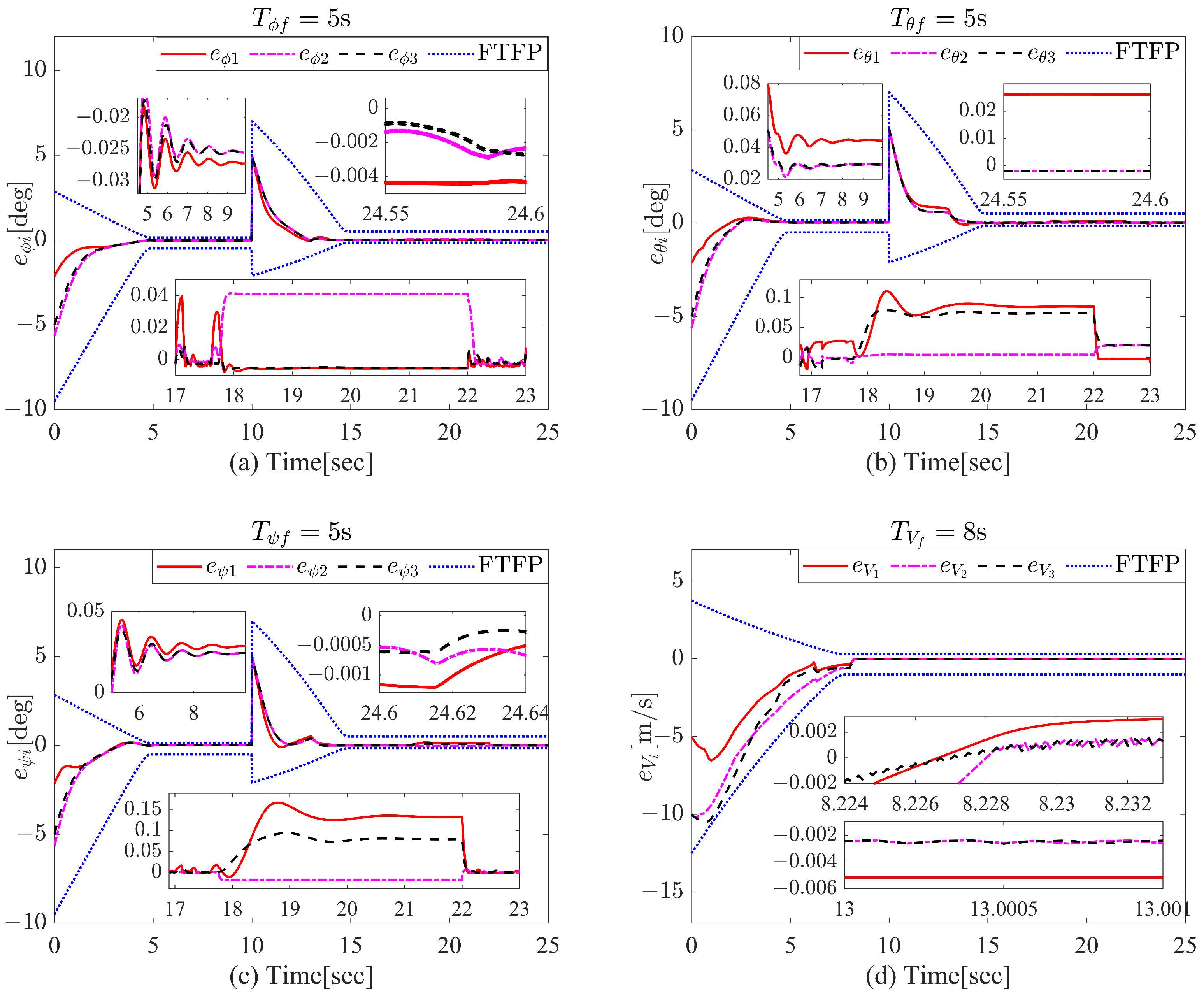
• All closed-loop signals are guaranteed to be SGUUB, and the synchronization tracking errors of both velocity and attitude are ensured to converge to a residual set around the origin within a fixed time.
• The velocity and attitude states remain within a set of time-varying asymmetric constraints. Specifically, for each UAV, both $V_i$ and ${\phi }_i$ satisfy the constraints ${\Gamma }_1=\left\{e_{vi}\right|-l_{vi}\left(t\right)<e_{vi}<h_{vi}\left(t\right),l_{vi}\left(t\right)>0\mathrm{and}{h}_{vi}\left(t\right)>0\}$ and ${\Gamma }_2=\left\{e_{mi}\right|-l_{mi}\left(t\right)<e_{mi}<h_{mi}\left(t\right),l_{mi}\left(t\right)>0\mathrm{and}{h}_{mi}\left(t\right)>0,m=\varphi ,\theta ,\psi \}$.

• For the convenience of derivation, the following definition and lemmas are needed.

Consider the following continuous nonlinear dynamic systems:

$$\dot{x}=f(t,x), x\left(t_0\right)=x_0$$

(23)

where $f(t,x):{\mathbb{R}}^{+}\times \mathbb{D}\to {\mathbb{R}}^n$ is a piecewise continuous function on ${\mathbb{R}}^{+}\times \mathbb{D}$ with respect to t, $f(t,x):{\mathbb{R}}^{+}\times \mathbb{D}\to {\mathbb{R}}^n$ is locally Lipschitz continuous with respect to x, and $\mathbb{D}\subset {\mathbb{R}}^n$ is the domain that contains the origin.

Definition 1.

The closed-loop signals of system (23) is said to be semi-globally uniformly ultimately bounded (SGUUB), if for a compact set $B_r\subset {\mathbb{R}}^n$ and any initial state $x_0= x\left(t_0\right)\in B_r$, there exist a positive constant p and continuously differentiable Lyapunov function $\mathcal{V}$, such that $\mathcal{V}\le p$, for $\forall t\ge 0$.

Assumption 4.

The reference signals, $V_r$, ${\mathit{\phi }}_r$, along with their second-order time derivatives, ${\ddot{V}}_r$, and ${\ddot{\mathit{\phi }}}_r$, are both continuous and bounded.

Lemma 2

([33]). For any scalars $c>0$ and $z\in \mathbb{R}$, the following equation is satisfied: $0\le \left|z\right|-{\displaystyle \frac{z^2}{\sqrt{z^2+c}}}\le \sqrt{c}$.

Lemma 3

([37]). For any scalars $c>0$ and $\vartheta \in \mathbb{R}$, the following equation holds $0\le \left|\vartheta \right|-\vartheta tanh\left({\displaystyle \frac{\vartheta }{c}}\right)\le 0.2785c$.

Lemma 4

([31]). For any two vectors $\mathit{x},\mathit{y}\in {\mathbb{R}}^N$, if there exist $c>0$ and $p, q \ge 1$ such that $(p-1)(q-1)=1$, then it holds that ${\mathit{x}}^{\mathrm{T}}\mathit{y}\le {\displaystyle \frac{c^p}{p}}{∥\mathit{x}∥}^p+{\displaystyle \frac{1}{q{c}^q}}{∥\mathit{y}∥}^q$.

3. Adaptive Fixed-Time Controller Design

3.1. Fixed-Time Performance Function

Definition 2.

A smooth function $\rho \left(t\right)$ is called fixed-time performance function (FTPF), if the following conditions are satisfied [38]:

• $\rho \left(t\right)$ is positive and decreasing over time for $t\in [0,T)$;
• $\rho \left(t\right)\equiv {\tau }_{\infty }>0$ for all $t\ge T$, where ${\tau }_{\infty }$ is a positive design parameter.

According to Definition 2, FTPF is constructed as

$$\begin{array}{c}\hfill \mathcal{K}\left(t\right)=\left\{\begin{array}{c}{\displaystyle \frac{e^{\theta \frac{t}{T-t}+r}+e^{-\theta \frac{t}{T-t}-r}}{e^{\theta \frac{t}{T-t}+r}-e^{-\theta \frac{t}{T-t}-r}}}-1+{\tau }_{\infty },t\in [0,T)\mathrm{s}\\ {\tau }_{\infty },t\in [T,+\infty )\mathrm{s}\end{array}\right.\end{array}$$

(24)

where ϑ and r are positive constants.

Proof. 

Referring to (24), it can be deduced that $\rho \left(T^{-}\right)={lim}_{t\to T^{-}}{\tau }_{\infty }-1+{\displaystyle \frac{e^{\theta \frac{t}{T-t}+r}+e^{-\theta \frac{t}{T-t}-r}}{e^{\theta \frac{t}{T-t}+r}-e^{-\theta \frac{t}{T-t}-r}}}={\tau }_{\infty }=\rho \left(T^{+}\right),$ which shows that $\rho \left(t\right)$ is continuous. Moreover, the time derivative of $\rho \left(t\right)$ when $t\in [0,T)$ is given by: $\dot{\rho }\left(t\right)=-{\displaystyle \frac{\vartheta }{T}}{\left({\displaystyle \frac{T}{T-t}}\right)}^2{\left({\displaystyle \frac{2}{e^{\theta \frac{t}{T-t}+r}-e^{-\theta \frac{t}{T-t}-r}}}\right)}^2,$ and $\dot{\rho }\left(t\right)=0$ when $t\in [T,+\infty )$. For simplicity, we define $x={\displaystyle \frac{t}{T-t}}$, and as $t\to T^{-}$, it holds that $x\to +\infty$. Thus, we obtain: ${lim}_{t\to T^{-}}\dot{\rho }\left(t\right)=-{\displaystyle \frac{\vartheta }{T}}{\left({\displaystyle \frac{T}{T-t}}\right)}^2{\left({\displaystyle \frac{2}{e^{\theta \frac{t}{T-t}+r}-e^{-\theta \frac{t}{T-t}-r}}}\right)}^2=\dot{\rho }\left(T^{+}\right).$ Additionally, the second derivative of ${\rho }^2\left(t\right)$ is given by: ${\displaystyle \frac{d{\rho }^2\left(t\right)}{d{t}^2}}=\sqrt{|\dot{\rho }\left(t\right)|}{\displaystyle \frac{4\sqrt{\vartheta /r}}{e^{\vartheta x+r}-e^{-\vartheta x-r}}}+{\displaystyle \frac{T}{4}}\dot{\rho }\left(t\right)\left(1+{\displaystyle \frac{2e^{-\vartheta x-r}}{e^{\vartheta x+r}-e^{-\vartheta x-r}}}\right).$ Therefore, it can be concluded that ${lim}_{t\to T^{-}}{\displaystyle \frac{d{\rho }^2\left(t\right)}{d{t}^2}}={\displaystyle \frac{d{\rho }^2\left(t\right)}{d{t}^2}}=0.$ Similarly, it follows that ${lim}_{t\to T^{-}}{\displaystyle \frac{d{\rho }^i\left(t\right)}{d{t}^2}}={\displaystyle \frac{d{\rho }^i\left(t\right)}{d{t}^2}}=0,i=3,\cdots ,n.$ This shows that $\rho \left(t\right)$ is a smooth function. Furthermore, $\dot{\rho }\left(t\right)\le 0$, and the function $\rho \left(t\right)$ remains continuous at T. Therefore, it can be concluded that $\rho \left(t\right)$ is an FTPF, which completes the proof. □

Figure 1 illustrates how parameter r adjusts the initial value of the FTPF, parameter $\theta$ controls the slope of the FTPF, parameter T determines the convergence time of the FTPF, and parameter ${\tau }_{\infty }$ affects the system’s convergence accuracy. The combined effect of the FTPF and tan-BLF is used to ensure that the tracking error does not exceed the FTPF boundary, while the preassigned convergence time does not exceed parameter T. Specifically, a smaller value of parameter r results in a smaller initial value, a smaller value of parameter $\theta$ leads to a smaller slope, and a smaller value of parameter T accelerates convergence. Furthermore, to apply the FTPF to each segment of the system’s control commands, $\left(t-a\right)$ can replace t in $\mathcal{K}\left(t\right)$, thereby imposing a state constraint on time $t\in [a,+\infty )$ and limiting the convergence time to within $[a,a+T]$. Additionally, considering that the definition of a closed-loop system signals being SGUUB requires the initial condition $x_0\left(t_0\right)\in B_r$, which corresponds to the initial error satisfying $-l\left(0\right)<e\left(0\right)<h\left(0\right)$, it is necessary to ensure that $\left|e\left(0\right)\right|<\mathcal{K}\left(0\right)$, i.e., $\left|e\left(0\right)\right|<\left(1+{\displaystyle \frac{2}{e^{2r}-1}}\right)$. For the convenience of evaluating $\left(1+2/\phantom{2\left(e^{2r}-1\right)}\left(e^{2r}-1\right)\right)$, let $\left(1+2/\phantom{2\left(e^{2r}-1\right)}\left(e^{2r}-1\right)\right)=m$, where $m>max\{1,e(0\left)\right\}$. From this, the following expression can be derived $r={\displaystyle \frac{In\left(\left(2/\phantom{2\left(m-1\right)}\left(m-1\right)\right)+1\right)}{2}}$. Therefore, it is sufficient to ensure that $\left|e\left(0\right)\right|<m$ and that $r={\displaystyle \frac{In\left(\left(2/\phantom{2\left(m-1\right)}\left(m-1\right)\right)+1\right)}{2}}$ in order to guarantee that the initial values of the system are not violated. The above discussion demonstrates that this performance function can accommodate any magnitude of initial error.

Remark 2.

While traditional fixed-time control (FTC) strategies overcome dependency on initial system states, a review of FTC approaches using constant exponential coefficients, such as in [28], shows that stability and convergence rates are dictated by terms like $l_1{\mathrm{sig}}^{r_1}\left(x\right)$ and $l_2{\mathrm{sig}}^{r_2}\left(x\right)$, with stability condition $V\left(x\right)⩽-a{V}^{r_1}\left(x\right)-b{V}^{r_2}\left(x\right)+\eta$, $a,b>0,r_1>0,r_2>0$. These terms limit flexibility in adjusting convergence rates and complicate controller design. Most studies focus on modifying the exponents $r_1$ and $r_2$ without eliminating reliance on them. For instance, in [27], Zhang et al. introduced an auxiliary variable $z_i$ along with two dynamic variables $r_1$ and $r_2$ to guarantee that the convergence time of the fixed-time control method meets the requirements for the exponential terms. In [29], Hao et al. proposed a multivariable timing control strategy based on a variable exponential function, where a single variable exponential function is sufficient to keep the exponential terms ${\alpha }_1$ and ${\alpha }_2$ within the required bounds. Nevertheless, despite the development of innovative exponential control functions, the dependence of the convergence time on the exponential terms ${\alpha }_1$ and ${\alpha }_2$ in traditional fixed-time control methods cannot be avoided. This, in turn, complicates the design of fixed-time control methods, making it difficult to develop simple and straightforward fixed-time controllers. Equation (24) introduces FTPF, removing the need for these terms. By integrating FTPF with a tan-type BLF, the convergence rate and time are more effectively controlled.

3.2. Controller Design and Stability Analysis

In this section, the controllers and adaptive laws for the translation and rotation of the ith UAV are designed using backstepping and adaptive control methods. By constructing a BLF, the tracking errors for translation and rotation are guaranteed to converge to the sets ${\Gamma }_1$ and ${\Gamma }_2$, respectively. Specifically, $T_{xi0}$ and ${\delta }_{i0}$ denote the controllers for the translation and rotation dynamics. Given the velocity reference trajectory $V_r$ and attitude reference trajectory ${\phi }_r$ for the ith UAV, the velocity and attitude tracking errors are defined as ${\tilde{V}}_i=V_i-V_r$ and ${\tilde{\phi }}_i={\phi }_i-{\phi }_r$, respectively. Based on the topological relationship between adjacent UAVs, the velocity and attitude adjacency errors $e_{vi}$ and $e_{\phi i}$ are defined as follows:

$$\begin{array}{cc}\hfill e_{vi}& ={\lambda }_{i1}{\tilde{V}}_i+{\lambda }_{i2}\sum _{j\in {\mathcal{M}}_i}{a}_{ij}\left({\tilde{V}}_i-{\tilde{V}}_j\right)\hfill \\ \hfill & =\left({\lambda }_{i1}+{\lambda }_{i2}\sum _{j\in {\mathcal{M}}_i}{a}_{ij}\right){\tilde{V}}_i-{\lambda }_{i2}\sum _{j\in {\mathcal{M}}_i}{a}_{ij}{\tilde{V}}_j\hfill \end{array}$$

(25)

$$\begin{array}{cc}\hfill {\mathit{e}}_{\phi i}& ={\lambda }_{i3}{\tilde{\mathit{\phi }}}_i+{\lambda }_{i4}\sum _{j\in {\mathcal{M}}_i}{a}_{ij}\left({\tilde{\mathit{\phi }}}_i-{\tilde{\mathit{\phi }}}_j\right)\hfill \\ & =\left({\lambda }_{i3}+{\lambda }_{i4}\sum _{j\in {\mathcal{M}}_i}{a}_{ij}\right){\tilde{\mathit{\phi }}}_i-{\lambda }_{i4}\sum _{j\in {\mathcal{M}}_i}{a}_{ij}{\tilde{\mathit{\phi }}}_j\hfill \end{array}$$

(26)

where ${\lambda }_{i1}$, ${\lambda }_{i2}$, ${\lambda }_{i3}$, and ${\lambda }_{i4}$ are positive constants regulating the velocity synchronization performance, and ${\mathit{e}}_{\phi i}={\left[e_{\varphi i},e_{\theta i},e_{\psi i}\right]}^{\mathrm{T}}$.

3.2.1. Translational Kinematics

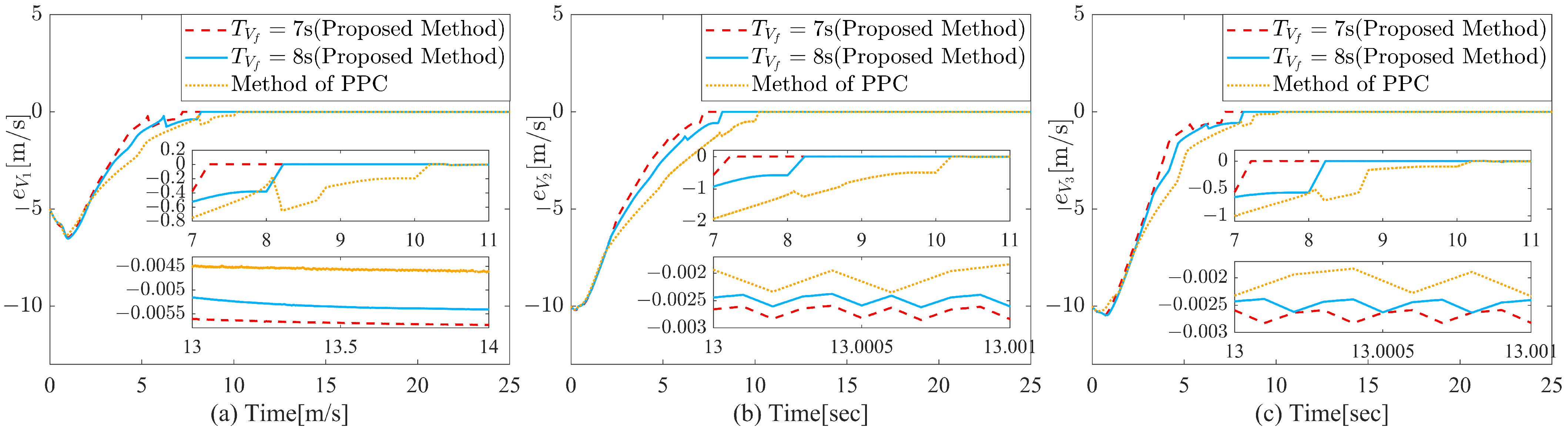
In this subsection, the FTPF is utilized to ensure that the UAV’s velocity converges within a fixed time. Furthermore, a modified segmented asymmetric tan-type BLF is designed to guarantee that the velocity adjacency error $e_{vi}$ remains within the set ${\Gamma }_1$ under asymmetric constraints. By differentiating $e_{vi}$, based on (12) and (25), the following expression is obtained:

$$\begin{array}{cc}\hfill {\dot{e}}_{vi}& =\left({\lambda }_{i1}+{\lambda }_{i2}\sum _{j\in {\mathcal{M}}_i}{a}_{ij}\right){\dot{\tilde{V}}}_i-{\lambda }_{i2}\sum _{j\in {\mathcal{M}}_i}{a}_{ij}{\dot{\tilde{V}}}_j\hfill \\ \hfill & ={\chi }_{vi}{\ell }_{Pi}{P}_{xi0}+{\chi }_{vi}{P}_{xif}+{\eta }_{vi}+{\Lambda }_1{\displaystyle \frac{v_i^{\mathrm{T}}}{V_i}}({\zeta }_{vi}+{\mathcal{D}}_{vi})\hfill \end{array}$$

(27)

where ${\Lambda }_1={\lambda }_{i1}+{\lambda }_{i2}{\displaystyle \sum _{j\in {\mathcal{M}}_i}}{a}_{ij}$, ${\chi }_{vi}={\displaystyle \frac{u_i{\Lambda }_{i1}}{m_i{V}_i}}$ and ${\eta }_{vi}={\Lambda }_1{\displaystyle \frac{{\mathit{v}}_i^T}{V_i}}\left({\mathcal{R}}_1^{\mathrm{T}}\left({\mathit{\phi }}_i\right)\mathit{g}+{\displaystyle \frac{{\mathcal{F}}_{i0}}{m_i}}\right)-{\Lambda }_1{\dot{V}}_r-{\lambda }_{i2}{\displaystyle \sum _{j\in {\mathcal{M}}_i}}{a}_{ij}{\dot{\tilde{V}}}_j$.

For the model uncertainty term ${\zeta }_{vi}$ in (27), a RBF NN is introduced to approximate ${\zeta }_{vi}$. Using Equation (21), we obtain

$$\begin{array}{cc}\hfill v_i^{\mathrm{T}}({\zeta }_{vi}+d_{vi})& =v_i^{\mathrm{T}}\left[\begin{array}{c}{\mathit{J}}_{vi1}^{*\mathrm{T}}{\mathit{S}}_{vi1}+{\mathcal{O}}_{vi1}+{\mathcal{D}}_{vi1}\\ {\mathit{J}}_{vi2}^{*\mathrm{T}}{\mathit{S}}_{vi2}+{\mathcal{O}}_{vi2}+{\mathcal{D}}_{vi2}\\ {\mathit{J}}_{vi3}^{*\mathrm{T}}{\mathit{S}}_{vi3}+{\mathcal{O}}_{vi3}+{\mathcal{D}}_{vi3}\end{array}\right]\hfill \\ \hfill & =\sum _{a=1}^3{v}_{ia}^T{\mathit{J}}_{via}^{*T}{\mathit{S}}_{via}+\sum _{a=1}^3{v}_{ia}^T({\mathcal{O}}_{via}+{\mathcal{D}}_{via})\hfill \end{array}$$

(28)

where $v_{ia}$ is an element of the vector $v_i$, represented as $v_i={\left[v_{i1},v_{i2},v_{i3}\right]}^{\mathrm{T}}$.

Using Lemma 4, we have

$$\begin{array}{cc}\hfill & {\displaystyle \frac{e_{vi}}{V_i}}{v}_{ia}^{\mathrm{T}}{\mathit{J}}_{via}^{*T}{\mathit{S}}_{via}\le {\displaystyle \frac{e_{vi}^2{v}_{ia}^2{\Phi }_{vi}{\mathit{S}}_{via}^{\mathrm{T}}{\mathit{S}}_{via}}{2{\varpi }_{v1}^2{V}_i^2}}+{\displaystyle \frac{{\varpi }_{v1}^2}{2}}\hfill \end{array}$$

(29)

$$\begin{array}{cc}\hfill & {\displaystyle \frac{e_{vi}}{V_i}}{v}_{ia}^{\mathrm{T}}({\tau }_{via}+{\mathcal{D}}_{via})\le {\displaystyle \frac{e_{vi}^2{v}_{ia}^2}{2{\varpi }_{v2}^2{V}_i^2}}+{\displaystyle \frac{{\varpi }_{v2}^2{\overline{\mathcal{D}}}_{via}^2}{2}}\hfill \end{array}$$

(30)

where ${\Phi }_{vi}=max\left\{{\mathit{J}}_{vi1}^{*\mathrm{T}}{\mathit{J}}_{vi1}^{*},{\mathit{J}}_{vi2}^{*\mathrm{T}}{\mathit{J}}_{vi2}^{*},{\mathit{J}}_{vi3}^{*\mathrm{T}}{\mathit{J}}_{vi3}^{*}\right\}$, and ${\mathcal{O}}_{via}+{\mathcal{D}}_{via}$ satisfies $\left|{\mathcal{O}}_{via}+{\mathcal{D}}_{via}\right|\le {\overline{\mathcal{D}}}_{via}$. Thus, we obtain:

$$\begin{array}{c}\hfill {\displaystyle \frac{e_{vi}}{V_i}}{\mathit{v}}_i^{\mathrm{T}}\left({\mathit{\zeta }}_{vi}+{\mathcal{D}}_{vi}\right)\le \sum _{a=1}^3\left({\displaystyle \frac{e_{vi}^2{v}_{ia}^2{\Phi }_{vi}{\mathit{S}}_{via}^{\mathrm{T}}{\mathit{S}}_{via}}{2{\varpi }_{vi1}^2{V}_i^2}}+{\displaystyle \frac{e_{vi}^2{v}_{ia}^2}{2{\varpi }_{vi2}^2{V}_i^2}}\right.+\left.{\displaystyle \frac{{\varpi }_{vi1}^2}{2}}+{\displaystyle \frac{{\varpi }_{vi2}^2{\overline{\mathcal{D}}}_{via}^2}{2}}\right)\end{array}$$

(31)

Define ${\mathbf{\Psi }}_{vi}=e_{vi}{[v_{i1}{\mathit{S}}_{vi1}^{\mathrm{T}}{\mathit{S}}_{vi1},v_{i2}{\mathit{S}}_{vi2}^{\mathrm{T}}{\mathit{S}}_{vi2},v_{i1}{\mathit{S}}_{vi3}^{\mathrm{T}}{\mathit{S}}_{vi3}]}^{\mathrm{T}}$. Then, when we substitute (31) into (27), one has

$$\begin{array}{c}\hfill e_{vi}{\dot{e}}_{vi}\le e_{vi}\left({\chi }_{vi}{\ell }_{Pi}{P}_{xi0}+{\chi }_{vi}{P}_{xif}+{\eta }_{vi}\right.+{\Lambda }_1{\displaystyle \frac{{\Phi }_{vi}{v}_i^{\mathrm{T}}{\mathbf{\Psi }}_{vi}}{2{\varpi }_{v1}^2{V}_i^2}}\left.+{\Lambda }_1{\displaystyle \frac{e_{vi}{v}_i^{\mathrm{T}}{v}_i}{2{\varpi }_{v2}^2{V}_i^2}}\right)+{\Lambda }_1\sum _{\mathrm{a}=1}^3\left({\displaystyle \frac{{\varpi }_{v1}^2}{2}}+{\displaystyle \frac{{\varpi }_{v2}^2{\overline{\mathcal{D}}}_{via}^2}{2}}\right)\end{array}$$

(32)

To address unknown actuator parameters, ${\wp }_{vi}=1/{\ell }_{Pi}$ and ${\Im }_{vi}={\wp }_{vi}{sup}_{t\ge 0}\left|P_{xif}\right|$ are defined. The unknown parameters ${\wp }_{vi}$, ${\Im }_{vi}$, and ${\Xi }_{vi}$ in (31) are handled through parameter update laws integrated into the controller $T_{xi0}$. This ensures fixed-time convergence of the UAV’s velocity despite uncertainties, external disturbances, and actuator failures. The parameter estimation errors are defined as ${\tilde{\wp }}_{vi}={\widehat{\wp }}_{vi}-{\wp }_{vi}$, ${\tilde{\Im }}_{vi}={\widehat{\Im }}_{vi}-{\Im }_{vi}$, and ${\tilde{\Xi }}_{vi}={\widehat{\Xi }}_{vi}-{\Xi }_{vi}$, where ${\widehat{\wp }}_{vi}$, ${\widehat{\Im }}_{vi}$, and ${\widehat{\Xi }}_{vi}$ are the estimated values.

The tan-type BLF is designed to ensure that the velocity adjacency error $e_{vi}\left(t\right)$ remains within the set ${\Gamma }_1=\left\{e_{vi}|-l_{vi}\left(t\right)<e_{vi}<h_{vi}\left(t\right),l_{vi}\left(t\right)>0,h_{vi}\left(t\right)\right.\left.>0\right\}$. To meet performance constraints, an improved segmented asymmetric tan-type BLF is constructed as follows:

$$\begin{array}{c}\hfill {\mathcal{V}}_1={\displaystyle \frac{l_{vi}^2\left(t\right)}{\pi }}{M}_{i,j}tan\left({\displaystyle \frac{\pi e_{vi}^2\left(t\right)}{2l_{vi}^2\left(t\right)}}\right)+{\displaystyle \frac{h_{vi}^2\left(t\right)}{\pi }}(1-M_{i,j})tan\left({\displaystyle \frac{\pi e_{vi}^2\left(t\right)}{2h_{vi}^2\left(t\right)}}\right)+{\displaystyle \frac{{\rho }_{Ti}}{2{\gamma }_{vi1}}}{\tilde{\wp }}_{vi}^2+{\displaystyle \frac{1}{2{\gamma }_{vi2}}}{\tilde{\Xi }}_{vi}^2+{\displaystyle \frac{{\rho }_{Ti}}{2{\gamma }_{vi3}}}{\tilde{\Im }}_{vi}^2\end{array}$$

(33)

where ${\mathcal{K}}_{vi}\left(t\right)$ is an FTPF defined in (24) and (33) satisfies

$$\left\{\begin{array}{c}{l}_{vi}\left(t\right)={\underline{\epsilon }}_{vi}{\mathcal{K}}_{vi}\left(t\right),\hfill \\ h_{vi}\left(t\right)={\overline{\epsilon }}_{vi}{\mathcal{K}}_{vi}\left(t\right),\hfill \end{array}\right.$$

$$\left\{\begin{array}{c}{\underline{\epsilon }}_{vi}=1\mathrm{and}0<{\overline{\epsilon }}_{vi}<1,\mathrm{if}{e}_{vi}\left(0\right)<0,\hfill \\ {\overline{\epsilon }}_{vi}=1\mathrm{and}0<{\underline{\epsilon }}_{vi}<1,\mathrm{if}{e}_{vi}\left(0\right)>0,\hfill \end{array}\right.$$

$$\left\{\begin{array}{c}{M}_{i,j}=1,e_{vi}\left(t\right)<0.\hfill \\ M_{i,j}=0,e_{vi}\left(t\right)>0.\hfill \end{array}\right.$$

For simplification, let ${{\rm Y}}_{vi1}={sec}^2\left({\displaystyle \frac{\pi e_{vi}^2}{2l_{vi}^2}}\right)$, ${{\rm Y}}_{vi2}={sec}^2\left({\displaystyle \frac{\pi e_{vi}^2}{2h_{vi}^2}}\right)$, and ${{\rm Y}}_{vi}=M_{vi}{{\rm Y}}_{vi1}+(1-M_{vi}){{\rm Y}}_{vi2}$. The partial derivative of $V_1$ is derived as follows:

$$\begin{array}{c}\hfill {\dot{\mathcal{V}}}_1={{\rm Y}}_{vi}{e}_{vi}{\dot{e}}_{vi}+{\displaystyle \frac{{\rho }_{Ti}}{{\gamma }_{vi1}}}{\tilde{\wp }}_{vi}{\dot{\widehat{\wp }}}_{vi}+{\displaystyle \frac{1}{{\gamma }_{vi2}}}{\tilde{\Xi }}_{vi}{\dot{\widehat{\Xi }}}_{vi}+{\displaystyle \frac{{\rho }_{Ti}}{{\gamma }_{vi3}}}{\tilde{\Im }}_{vi}{\dot{\widehat{\Im }}}_{vi}\end{array}$$

(34)

Remark 3.

The tan-type BLF is effectively used to address full-state constraints in dynamic systems by transforming state constraints into tracking error constraints through backstepping techniques. However, previous research has primarily concentrated on symmetric, time-invariant tan-type BLFs. In practical engineering, systems often require specific prescribed performance constraints, where tracking errors must converge to an arbitrarily small residual set at a rate exceeding a defined threshold. To achieve this, symmetric tan-type BLFs are typically combined with Prescribed Performance Control (PPC) to regulate tracking errors [39]. Nevertheless, the PPC performance function, $\rho \left(t\right)=\left({\tau }_{\rho }-{\tau }_{\infty }\right)exp\left(-l_{\rho }t\right)+{\tau }_{\infty }$, does not specify a convergence time, limiting its precision in performance control [14,18]. Additionally, the symmetry of the tan-type BLFs reduces flexibility in selecting initial conditions, making this approach overly conservative for addressing performance constraints. A segmented, asymmetric tan-type BLF with FTPF is thus proposed in Equation (33) to overcome these limitations.

Remark 4.

According to the form of the designed BLF in (33), when $l_{vi}$ and $h_{vi}$ tend to infinity, the following limit can be deduced: ${lim}_{k_{vi}\to \infty }\left(M_{vi}{\displaystyle \frac{l_{vi}^2}{\pi }}tan\left({\displaystyle \frac{\pi e_{vi}^2}{2l_{vi}^2}}\right)\right.$$\left.+(1-M_{vi}){\displaystyle \frac{h_{vi}^2}{\pi }}tan\left({\displaystyle \frac{\pi e_{vi}^2}{2h_{vi}^2}}\right)\right)={\displaystyle \frac{1}{2}}{e}_{vi}^2$ This indicates that the adjacency tracking error $e_{vi}\left(t\right)$ becomes unconstrained. Therefore, the analysis method proposed in this paper can be extended to unconstrained cases. Furthermore, since both the numerator and denominator powers are positive even numbers, it follows that $0<{\displaystyle \frac{\pi e_{vi}^2\left(t\right)}{2l_{vi}^2\left(t\right)}}<{\displaystyle \frac{\pi }{2}}$ and $0<{\displaystyle \frac{\pi e_{vi}^2\left(t\right)}{2h_{vi}^2\left(t\right)}}<{\displaystyle \frac{\pi }{2}}$, meaning that issues of singularity are absent, and the designed barrier Lyapunov function (BLF) remains effective as the error approaches zero.

Substituting (32) into (34), we obtain

$$\begin{array}{cc}\hfill {\dot{\mathcal{V}}}_1\le & {\Lambda }_1\sum _{\mathrm{a}=1}^3\left({\displaystyle \frac{{\varpi }_{v1}^2}{2}}+{\displaystyle \frac{{\varpi }_{v2}^2{\overline{d}}_{via}^2}{2}}\right)+{\displaystyle \frac{{\ell }_{Pi}}{{\gamma }_{vi1}}}{\tilde{\wp }}_{vi}{\dot{\widehat{\wp }}}_{vi}+{\displaystyle \frac{1}{{\gamma }_{vi2}}}{\tilde{\Xi }}_{vi}{\dot{\widehat{\Xi }}}_{vi}+{\displaystyle \frac{{\ell }_{Pi}}{{\gamma }_{vi3}}}{\tilde{\Im }}_{vi}{\dot{\widehat{\Im }}}_{vi}\hfill \\ & +{{\rm Y}}_{vi}{e}_{vi}\left({\chi }_{vi}{\ell }_{Pi}{P}_{xi0}+{\chi }_{vi}{P}_{xif}+{\eta }_{vi}+{\Lambda }_1{\displaystyle \frac{{\Phi }_{vi}{v}_i^{\mathrm{T}}{\mathbf{\Psi }}_{\mathit{vi}}}{2{\varpi }_{v1}^2{V}_i^2}}\right.\left.+{\Lambda }_1{\displaystyle \frac{e_{vi}{v}_i^{\mathrm{T}}{v}_i}{2{\varpi }_{v2}^2{V}_i^2}}\right)\hfill \end{array}$$

(35)

Let ${\alpha }_{vi}={\eta }_{vi}+{\Lambda }_1{\displaystyle \frac{{\widehat{\Phi }}_{vi}{v}_i^{\mathrm{T}}{\mathbf{\Psi }}_{\mathit{vi}}}{2{\varpi }_{v1}^2{V}_i^2}}+{\Lambda }_1{\displaystyle \frac{e_{vi}^2{v}_i^{\mathrm{T}}{v}_i}{2{\varpi }_{v2}^2{V}_i^2}}$, then (35) is reformulated as

$$\begin{array}{c}\hfill {\dot{\mathcal{V}}}_1\le {{\rm Y}}_{vi}{e}_{vi}\left({\chi }_{vi}{\ell }_{Pi}{P}_{xi0}+{\chi }_{vi}{P}_{xif}+{\alpha }_{vi}\right)+{\Lambda }_1\sum _{\mathrm{a}=1}^3\left({\displaystyle \frac{{\varpi }_{v1}^2}{2}}+{\displaystyle \frac{{\varpi }_{v2}^2{\overline{\mathcal{D}}}_{via}^2}{2}}\right)+{\displaystyle \frac{{\ell }_{Pi}}{{\gamma }_{vi1}}}{\tilde{\wp }}_{vi}{\dot{\widehat{\wp }}}_{vi}+{\displaystyle \frac{1}{{\gamma }_{vi2}}}{\tilde{\Xi }}_{vi}{\dot{\widehat{\Xi }}}_{vi}+{\displaystyle \frac{{\ell }_{Pi}}{{\gamma }_{vi3}}}{\tilde{\Im }}_{vi}{\dot{\widehat{\Im }}}_{vi}\end{array}$$

(36)

According to Lemma 3 and ${\Im }_{vi}={\wp }_{vi}{sup}_{t\ge 0}\left|P_{xif}\right|$, the term ${{\rm Y}}_{vi}{e}_{vi}{\chi }_{vi}{P}_{xif}$ satisfies

$$\begin{array}{c}\hfill {{\rm Y}}_{vi}{e}_{vi}{\chi }_{vi}{P}_{xif}\le {{\rm Y}}_{vi}{e}_{vi}{\chi }_{vi}{\ell }_{Pi}{\widehat{\Im }}_{vi}tanh\left({\displaystyle \frac{{{\rm Y}}_{vi}{e}_{vi}{\chi }_{vi}{\widehat{\Im }}_{vi}}{c_{vi}}}\right)+0.2785{\ell }_{Pi}{c}_{vi}-{{\rm Y}}_{vi}{e}_{vi}{\chi }_{vi}{\ell }_{Pi}{\tilde{\Im }}_{vi}\end{array}$$

(37)

where $c_{vi}>0$ is the parameter to be designed.

The thrust control law $P_{xi0}$ is designed as follows:

$$\begin{array}{cc}\hfill P_{xi0}=& -{\displaystyle \frac{{\mu }_{vi}{k}_{vi}^2}{\pi {\chi }_{vi}{\ell }_{Pi}{e}_{vi}}}(1-M_{vi})sin\left({\displaystyle \frac{\pi e_{vi}^2}{2h_{vi}^2}}\right)cos\left({\displaystyle \frac{\pi e_{vi}^2}{2h_{vi}^2}}\right)-{\widehat{\Im }}_{vi}tanh\left({\displaystyle \frac{{{\rm Y}}_{vi}{e}_{vi}{\chi }_{vi}{\widehat{\Im }}_{vi}}{c_{vi}}}\right)\hfill \\ \hfill & -{\displaystyle \frac{{\mu }_{vi}{k}_{vi}^2}{\pi {\chi }_{vi}{\ell }_{Pi}{e}_{vi}}}{M}_{vi}sin\left({\displaystyle \frac{\pi e_{vi}^2}{2l_{vi}^2}}\right)cos\left({\displaystyle \frac{\pi e_{vi}^2}{2l_{vi}^2}}\right)-{\displaystyle \frac{{\alpha }_{vi}{\widehat{\wp }}_{vi}}{{\chi }_{vi}}}tanh\left({\displaystyle \frac{e_{vi}{{\rm Y}}_{vi}{\alpha }_{vi}{\widehat{\wp }}_{vi}}{c_{vi}}}\right)\hfill \end{array}$$

(38)

For parameters ${\wp }_{vi}$, ${\Im }_{vi}$ and ${\Phi }_{vi}$, adaptive parameter update laws are defined as

$$\begin{array}{cc}\hfill {\dot{\widehat{\wp }}}_{vi}& ={\gamma }_{vi1}{{\rm Y}}_{vi}{e}_{vi}{\alpha }_{vi}-{\gamma }_{vi1}{\sigma }_{vi1}{\widehat{\wp }}_{vi}\hfill \end{array}$$

(39)

$$\begin{array}{cc}\hfill {\dot{\widehat{\Xi }}}_{vi}& ={\Lambda }_1{\displaystyle \frac{{\gamma }_{vi2}{{\rm Y}}_{vi}{e}_{vi}{v}_i^{\mathrm{T}}{\mathbf{\Psi }}_{\mathit{vi}}}{2{\varpi }_{v1}^2{V}_i^2}}-{\gamma }_{vi2}{\sigma }_{vi2}{\widehat{\Xi }}_{vi}\hfill \end{array}$$

(40)

$$\begin{array}{cc}\hfill {\dot{\widehat{\Im }}}_{vi}& ={\gamma }_{vi3}{{\rm Y}}_{vi}{e}_{vi}{\chi }_{vi}-{\gamma }_{vi3}{\sigma }_{vi3}{\widehat{\Im }}_{vi}\hfill \end{array}$$

(41)

where ${\gamma }_{vi1}$, ${\gamma }_{vi2}$, ${\gamma }_{vi3}$, ${\sigma }_{vi1}$, ${\sigma }_{vi2}$ and ${\sigma }_{vi3}$ are positive parameters to be designed.

Theorem 1.

Considering the translational kinematics with asymmetric time-varying constraints, and assuming that conditions 1-3 hold, the application of the controller designed in (38) and the adaptive laws in (39)–(41), for $-l_{vi}\left(0\right)<e\left(0\right)<h_{vi}\left(0\right)$, $\forall p_1>0$ and ${\mathcal{V}}_1\left(0\right)\le p$, the following properties hold:

• The closed-loop signals $e_{vi},{\tilde{\wp }}_{vi},{\tilde{\Xi }}_{vi}$ and ${\tilde{\Im }}_{vi}$ are guaranteed to be SGUUB and the synchronization tracking errors of velocity converges to a residual set around origin within a fixed time.
• The state of velocity is consistently within a set of time-varying asymmetric constraints.

Proof. 

According to Lemma 4 and (38), the term ${{\rm Y}}_{vi}{e}_{vi}{\chi }_{vi}{\rho }_{Ti}{T}_{xi0}$ satisfies

$$\begin{array}{cc}\hfill {{\rm Y}}_{vi}{e}_{vi}{\chi }_{vi}{\ell }_{Pi}{P}_{xi0}\le & -{{\rm Y}}_{vi}{e}_{vi}{\chi }_{vi}{\ell }_{Pi}{\widehat{\Im }}_{vi}tanh\left({\displaystyle \frac{{{\rm Y}}_{vi}{e}_{vi}{\chi }_{vi}{\rho }_{Pi}{\widehat{\Im }}_{vi}}{{\rho }_{Ti}{c}_{vi}}}\right)+0.2785{\ell }_{Pi}{c}_{vi}\hfill \\ & -{\displaystyle \frac{{\mu }_{vi}{h}_{vi}^2}{\pi }}(1-M_{vi})tan\left({\displaystyle \frac{\pi e_{vi}^2}{2h_{vi}^2}}\right)-{\displaystyle \frac{{\mu }_{vi}{l}_{vi}^2}{\pi }}{M}_{vi}tan\left({\displaystyle \frac{\pi e_{vi}^2}{2l_{vi}^2}}\right)\hfill \end{array}$$

(42)

Substituting (37) and (42) into (36), we obtain

$$\begin{array}{cc}\hfill {\dot{\mathcal{V}}}_1\le & -{\displaystyle \frac{{\mu }_{vi}{l}_{vi}^2}{\pi }}{M}_{vi}tan\left({\displaystyle \frac{\pi e_{vi}^2}{2l_{vi}^2}}\right)-{\displaystyle \frac{{\mu }_{vi}{h}_{vi}^2}{\pi }}(1-M_{vi})tan\left({\displaystyle \frac{\pi e_{vi}^2}{2h_{vi}^2}}\right)\hfill \\ & +{\displaystyle \frac{1}{{\gamma }_{vi2}}}{\tilde{\Xi }}_{vi}\left({\dot{\widehat{\Xi }}}_{vi}-{\Lambda }_1{\displaystyle \frac{{\gamma }_{vi2}{{\rm Y}}_{vi}{e}_{vi}{v}_i^{\mathrm{T}}{\mathbf{\Psi }}_{\mathit{vi}}}{2{\varpi }_{v1}^2{V}_i^2}}\right)\hfill \\ & +{\displaystyle \frac{{\ell }_{Ti}}{{\gamma }_{vi1}}}{\tilde{\wp }}_{vi}\left({\dot{\widehat{\wp }}}_{vi}-{\gamma }_{vi1}{{\rm Y}}_{vi}{e}_{vi}{\alpha }_{vi}\right)\hfill \\ & +{\displaystyle \frac{{\ell }_{Ti}}{{\gamma }_{vi3}}}{\tilde{\Im }}_{vi}\left({\dot{\widehat{\Im }}}_{vi}-{\gamma }_{vi3}{{\rm Y}}_{vi}{e}_{vi}{\chi }_{vi}\right)\hfill \\ & +{\Lambda }_1\sum _{\mathrm{a}=1}^3\left({\displaystyle \frac{{\varpi }_{v1}^2}{2}}+{\displaystyle \frac{{\varpi }_{v2}^2{\overline{\mathcal{D}}}_{via}^2}{2}}\right)\hfill \end{array}$$

(43)

Substituting (39)–(41) into (43), we obtain

$$\begin{array}{cc}\hfill {\dot{\mathcal{V}}}_1\le & -{\displaystyle \frac{{\mu }_{vi}{l}_{vi}^2}{\pi }}{M}_{vi}tan\left({\displaystyle \frac{\pi e_{vi}^2}{2l_{vi}^2}}\right)-{\displaystyle \frac{{\mu }_{vi}{h}_{vi}^2}{\pi }}(1-M_{vi})tan\left({\displaystyle \frac{\pi e_{vi}^2}{2h_{vi}^2}}\right)\hfill \\ & -{\ell }_{Pi}{\sigma }_{vi1}{\tilde{\wp }}_{vi}{\widehat{\wp }}_{vi}-{\ell }_{Pi}{\sigma }_{vi1}{\tilde{\Im }}_{vi}{\widehat{\Im }}_{vi}-{\sigma }_{vi1}{\tilde{\Xi }}_{vi}{\widehat{\Xi }}_{vi}\hfill \\ & +0.557{\ell }_{Pi}{c}_{vi}+{\Lambda }_1\sum _{\mathrm{a}=1}^3\left({\displaystyle \frac{{\varpi }_{v1}^2}{2}}+{\displaystyle \frac{{\varpi }_{v2}^2{\overline{\mathcal{D}}}_{via}^2}{2}}\right)\hfill \end{array}$$

(44)

Applying Lemma 4 to the term ${\tilde{\wp }}_{vi}{\widehat{\wp }}_{vi}$, ${\tilde{\Im }}_{vi}{\widehat{\Im }}_{vi}$ and ${\tilde{\Xi }}_{vi}{\widehat{\Xi }}_{vi}$, one has $-{\tilde{\wp }}_{vi}{\widehat{\wp }}_{vi}\le -{\displaystyle \frac{1}{2}}{\tilde{\wp }}_{vi}^2+{\displaystyle \frac{1}{2}}{\wp }_{vi}^2$, $-{\tilde{\Im }}_{vi}{\tilde{\Im }}_{vi}\le -{\displaystyle \frac{1}{2}}{\tilde{\Im }}_{vi}^2+{\displaystyle \frac{1}{2}}{\Im }_{vi}^2$ and $-{\tilde{\Xi }}_{vi}{\widehat{\Xi }}_{vi}\le -{\displaystyle \frac{1}{2}}{\tilde{\Xi }}_{vi}^2+{\displaystyle \frac{1}{2}}{\Xi }_{vi}^2$. Then it yields that

$$\begin{array}{cc}\hfill {\dot{\mathcal{V}}}_1\le & -{\displaystyle \frac{{\mu }_{vi}{l}_{vi}^2}{\pi }}{M}_{vi}tan\left({\displaystyle \frac{\pi e_{vi}^2}{2l_{vi}^2}}\right)-{\displaystyle \frac{{\mu }_{vi}{h}_{vi}^2}{\pi }}(1-M_{vi})tan\left({\displaystyle \frac{\pi e_{vi}^2}{2h_{vi}^2}}\right)\hfill \\ & +0.557{\ell }_{Pi}{c}_{vi}+{\Lambda }_1\sum _{\mathrm{a}=1}^3\left({\displaystyle \frac{{\varpi }_{v1}^2}{2}}+{\displaystyle \frac{{\varpi }_{v2}^2{\overline{\mathcal{D}}}_{via}^2}{2}}\right)\hfill \\ & -{\displaystyle \frac{{\ell }_{Pi}{\sigma }_{vi1}}{2}}{\tilde{\wp }}_{vi}^2-{\displaystyle \frac{{\sigma }_{vi2}}{2}}{\tilde{\Xi }}_{vi}^2-{\displaystyle \frac{{\ell }_{Pi}{\sigma }_{vi3}}{2}}{\tilde{\Im }}_{vi}^2\hfill \\ & +{\displaystyle \frac{{\ell }_{Pi}{\sigma }_{vi1}}{2}}{\wp }_{vi}^2+{\displaystyle \frac{{\sigma }_{vi2}}{2}}{\Xi }_{vi}^2+{\displaystyle \frac{{\ell }_{Pi}{\sigma }_{vi3}}{2}}{\Im }_{vi}^2\hfill \\ & \le -{\kappa }_{1i}{\mathcal{V}}_1+{\varsigma }_{1i}\hfill \end{array}$$

(45)

where ${\kappa }_{1i}=min\{{\mu }_{vi},{\gamma }_{vi1}{\sigma }_{vi1},{\gamma }_{vi2}{\sigma }_{vi2},{\gamma }_{vi3}{\sigma }_{vi3}\}$ and ${\varsigma }_{1i}={\displaystyle \frac{{\ell }_{Pi}{\sigma }_{vi1}}{2}}{\wp }_{vi}^2+{\displaystyle \frac{{\sigma }_{vi2}}{2}}{\Xi }_{vi}^2+{\displaystyle \frac{{\ell }_{Pi}{\sigma }_{vi3}}{2}}{\Im }_{vi}^2+0.557{\ell }_{Pi}{c}_{vi}+{\Lambda }_1{\displaystyle \sum _{\mathrm{a}=1}^3}\left({\displaystyle \frac{{\varpi }_{v1}^2}{2}}+{\displaystyle \frac{{\varpi }_{v2}^2{\overline{\mathcal{D}}}_{via}^2}{2}}\right)$.

From (45), it follows that

$$\begin{array}{c}\hfill 0\le {\mathcal{V}}_1\le [{\displaystyle \frac{{\varsigma }_{1i}}{{\kappa }_{1i}}}+{\mathcal{V}}_1\left(0\right)]e^{-{\kappa }_{1i}t}+{\displaystyle \frac{{\varsigma }_{1i}}{{\kappa }_{1i}}}\end{array}$$

(46)

Inequality (46) demonstrates that ${\mathcal{V}}_1$ is ultimately constrained by ${\displaystyle \frac{{\varsigma }_{1i}}{{\kappa }_{1i}}}$, and that ${\displaystyle \frac{{\varsigma }_{1i}}{{\kappa }_{1i}}}$ can be made arbitrarily small by simultaneously increasing ${\mu }_{vi},{\gamma }_{vi1}{\sigma }_{vi1},{\gamma }_{vi2}{\sigma }_{vi2},{\gamma }_{vi3}{\sigma }_{vi3}$ and decreasing $h_{vi1},h_{vi2},{\sigma }_{vi1},{\sigma }_{vi2},{\sigma }_{vi3},c_{vi}$. Moreover, by appropriately selecting the design parameters, ${\displaystyle \frac{{\varsigma }_{1i}}{{\kappa }_{1i}}}\le p_1$ can be achieved. When ${\mathcal{V}}_1=p_1$ is satisfied, Equation (45) leads to $\dot{{\mathcal{V}}_1}\le 0$, and when ${\displaystyle \frac{{\varsigma }_{1i}}{{\kappa }_{1i}}}\le p_1$ holds, ${\mathcal{V}}_1\le p_1$ holds for $\forall t\ge 0$. Consequently, the closed-loop signals $e_{vi},{\tilde{\wp }}_{vi},{\tilde{\Xi }}_{vi},{\tilde{\Im }}_{vi}$ in the translation subsystem are guaranteed to be SGUUB. This completes the proof of Theorem 1. □

3.2.2. Rotational Kinematics

In this subsection, the FTPF function is employed to ensure rapid convergence of the UAV’s attitude within a fixed time frame. Additionally, an improved tan-type barrier Lyapunov function (BLF) is designed to ensure that the attitude adjacency error ${\mathit{e}}_{\phi i}$ remains within the set ${\Gamma }_2$ under asymmetric constraints.

Step 1. Based on (16) and (26), differentiate ${\mathit{e}}_{\phi i}$ to obtain

$$\begin{array}{cc}\hfill {\dot{\mathit{e}}}_{\phi i}& =\left({\lambda }_{i3}+{\lambda }_{i4}\sum _{j\in {\mathcal{M}}_i}{a}_{ij}\right){\dot{\tilde{\mathit{\phi }}}}_i-{\lambda }_{i4}\sum _{j\in {\mathcal{M}}_i}{a}_{ij}{\dot{\tilde{\mathit{\phi }}}}_j\hfill \\ & ={\Lambda }_2({\mathcal{R}}_2^{-1}\left({\mathit{\phi }}_i\right){\mathit{\omega }}_i-{\dot{\mathit{\phi }}}_r)-{\lambda }_{i4}\sum _{j\in {\mathcal{M}}_i}{a}_{ij}{\dot{\tilde{\mathit{\phi }}}}_j\hfill \end{array}$$

(47)

To ensure that the attitude adjacency error $e_{\phi i}\left(t\right)$ remains within the set ${\Gamma }_2=\{e_{mi}\mid -l_{mi}\left(t\right)<e_{mi}<h_{mi}\left(t\right),l_{mi}\left(t\right)>0\mathrm{and}{h}_{mi}\left(t\right)>0,m=\varphi ,\theta ,\psi \}$, the following asymmetric BLF Lyapunov function is introduced:

$$\begin{array}{c}\hfill {\mathcal{V}}_2={\mathcal{V}}_{2\varphi }+{\mathcal{V}}_{2\theta }+{\mathcal{V}}_{2\psi }\end{array}$$

(48)

where for ${\mathcal{V}}_{2m}$, $m=\{\varphi ,\theta ,\psi \}$, there is

$$\begin{array}{c}\hfill {\mathcal{V}}_{2m}={\displaystyle \frac{h_{mi}^2\left(t\right)}{\pi }}(1-M_{mi})tan\left({\displaystyle \frac{\pi e_{mi}^2\left(t\right)}{2h_{mi}^2\left(t\right)}}\right)+{\displaystyle \frac{l_{mi}^2\left(t\right)}{\pi }}{M}_{mi}tan\left({\displaystyle \frac{\pi e_{mi}^2\left(t\right)}{2l_{mi}^2\left(t\right)}}\right)\end{array}$$

(49)

where ${\mathcal{K}}_{mi}\left(t\right)$ is an FTPF given in (24) and

$$\left\{\begin{array}{c}{l}_{mi}\left(t\right)={\underline{\epsilon }}_{mi}{\mathcal{K}}_{mi}\left(t\right),\hfill \\ h_{mi}\left(t\right)={\overline{\epsilon }}_{mi}{\mathcal{K}}_{mi}\left(t\right),\hfill \end{array}\right.$$

$$\left\{\begin{array}{c}{\underline{\epsilon }}_{mi}=1\mathrm{and}0<{\overline{\epsilon }}_{mi}<1,\mathrm{if}{e}_{mi}\left(0\right)<0,\hfill \\ {\overline{\epsilon }}_{mi}=1\mathrm{and}0<{\underline{\epsilon }}_{mi}<1,\mathrm{if}{e}_{mi}\left(0\right)>0,\hfill \end{array}\right.$$

$$\left\{\begin{array}{c}{M}_{mi}=1,\mathrm{if}{e}_{mi}\left(t\right)<0.\hfill \\ M_{mi}=0,\mathrm{if}{e}_{mi}\left(t\right)>0.\hfill \end{array}\right.$$

For the sake of simplicity in deduction, the following definition is introduced:

$$\begin{array}{c}\hfill {\mathit{{\rm Y}}}_{\phi i}={\mathit{M}}_{\phi i}{\mathit{{\rm Y}}}_{\phi i1}+(\mathit{I}-{\mathit{M}}_{\phi i}){\mathit{{\rm Y}}}_{\phi i2}\end{array}$$

(50)

where for ${\mathit{{\rm Y}}}_{\phi i1}=\mathrm{diag}\left[{{\rm Y}}_{\varphi i1},{{\rm Y}}_{\theta i1},{{\rm Y}}_{\psi i1}\right]$, there is ${{\rm Y}}_{mi1}={sec}^2\left({\displaystyle \frac{\pi e_{mi}^2}{2l_{mi}^2}}\right)$, and for ${\mathit{{\rm Y}}}_{\phi i2}=\mathrm{diag}\left[{{\rm Y}}_{\varphi i2},{{\rm Y}}_{\theta i2},{{\rm Y}}_{\psi i2}\right]$, there is ${{\rm Y}}_{mi2}={sec}^2\left({\displaystyle \frac{\pi e_{mi}^2}{2h_{mi}^2}}\right)$.

Using (48), (49), and (50), and by differentiating $V_2$, the following expression is derived:

$$\begin{array}{c}\hfill \begin{array}{c}\hfill {\dot{\mathcal{V}}}_2=\left({\mathit{H}}_{\phi i}^{\mathrm{T}}(\mathit{I}-{\mathit{M}}_{\phi i})+{\mathit{L}}_{\phi i}^{\mathrm{T}}{\mathit{M}}_{\phi i}\right){\mathit{{\rm Y}}}_{\phi i}{\mathit{E}}_{\phi i}\left({\Lambda }_2({\mathit{R}}_2^{-1}\left({\phi }_i\right){\mathit{\omega }}_i-{\dot{\mathit{\phi }}}_r)-{\lambda }_{i4}\sum _{j\in {\mathcal{M}}_i}{a}_{ij}{\dot{\tilde{\mathit{\phi }}}}_j\right)\end{array}\end{array}$$

(51)

where $\mathit{I}=\mathrm{diag}\{1,1,1\}$, ${\mathit{P}}_{\phi i}=\mathrm{diag}\{P_{\varphi i},P_{\theta i},P_{\psi i}\}$, ${\mathit{H}}_{\phi i}={[h_{\varphi },h_{\theta },h_{\psi }]}^{\mathrm{T}}$, ${\mathit{L}}_{\phi i}={[l_{\varphi },l_{\theta },l_{\psi }]}^{\mathrm{T}}$ and ${\mathit{E}}_{\phi i}=\mathrm{diag}\{e_{\varphi },e_{\theta },e_{\psi }\}$

Subsequently, the virtual control law is designed as follows:

$$\begin{array}{c}\hfill {\omega }_{di}={\displaystyle \frac{{\mathcal{R}}_2}{{\Lambda }_2}}\left(-{\displaystyle \frac{{\mathit{\mu }}_{\phi i}}{\pi }}{\mathit{\delta }}_{\phi i}{\mathit{M}}_{\phi i}{\mathit{S}}_{\phi i}{\mathit{C}}_{\phi i}{\mathit{L}}_{\phi i}-{\displaystyle \frac{{\mathit{\mu }}_{\phi i}}{\pi }}{\mathit{\delta }}_{\phi i}(\mathit{I}-{\mathit{M}}_{\phi i}){\mathit{S}}_{\phi i}^{\prime }{\mathit{C}}_{\phi i}^{\prime }{\mathit{H}}_{\phi i}\right.\left.+{\lambda }_{i4}\sum _{j\in {\mathcal{M}}_i}{a}_{ij}{\dot{\tilde{\phi }}}_j+{\Lambda }_2{\dot{\phi }}_r\right)\end{array}$$

(52)

where for ${\mathit{S}}_{\phi i}=\mathrm{diag}\left[S_{\varphi i},S_{\theta i},S_{\psi i}\right],{\mathit{C}}_{\phi i}=\mathrm{diag}\left[C_{\varphi i},C_{\theta i},C_{\psi i}\right]$, ${\mathit{\delta }}_{\phi i}=\mathrm{diag}\left[{\delta }_{\varphi i},{\delta }_{\theta i},\right.$$\left.{\delta }_{\psi i}\right]$, there is $S_{mi}=sin\left({\displaystyle \frac{\pi e_{mi}^2}{2l_{mi}^2}}\right)$, $C_{mi}=cos\left({\displaystyle \frac{\pi e_{mi}^2}{2l_{mi}^2}}\right)$, ${\delta }_{mi}={\displaystyle \frac{1}{e_{mi}}}$ and ${\mathit{\mu }}_{\phi i}\in {\mathbb{R}}^{3\times 3}$ are real diagonal matrices.

Similarly, for ${\mathit{S}}_{\phi i}^{\prime }=\mathrm{diag}\left[S_{\varphi i}^{\prime },S_{\theta i}^{\prime },S_{\psi i}^{\prime }\right],{\mathit{C}}_{\phi i}^{\prime }=\mathrm{diag}\left[C_{\varphi i}^{\prime },C_{\theta i}^{\prime },C_{\psi i}^{\prime }\right]$ in (52), there is $S_{mi}^{\prime }=sin\left({\displaystyle \frac{\pi e_{mi}^2}{2h_{mi}^2}}\right)$, $C_{mi}^{\prime }=cos\left({\displaystyle \frac{\pi e_{mi}^2}{2h_{mi}^2}}\right)$.

Let ${\mathit{e}}_{\omega i}={\mathit{\omega }}_i-{\mathit{\omega }}_{di}$, and by substituting (52) into (51), we obtain

$$\begin{array}{cc}\hfill {\dot{\mathcal{V}}}_2=& -{\left({\mathit{L}}_{\phi i}^{\mathrm{T}}{\mathit{M}}_{\phi i}+{\mathit{H}}_{\phi i}^{\mathrm{T}}(\mathit{I}-{\mathit{M}}_{\phi i})\right)}^{\mathrm{T}}(\mathit{I}-{\mathit{M}}_{\phi i}){\displaystyle \frac{{\mathit{\mu }}_{\phi i}}{\pi }}{\mathit{T}}_{\phi i}^{\prime }{\mathit{H}}_{\phi i}\hfill \\ \hfill & +\left({\mathit{H}}_{\phi i}^T(\mathit{I}-{\mathit{M}}_{\phi i})+{\mathit{L}}_{\phi i}^T{\mathit{M}}_{\phi i}\right){\mathit{{\rm Y}}}_{\phi i}{\mathit{E}}_{\phi i}{\Lambda }_2{\mathit{R}}_2^{-1}\left({\mathit{\phi }}_i\right){\mathit{e}}_{\omega i}\hfill \\ \hfill & -{\left({\mathit{L}}_{\phi i}^{\mathrm{T}}{\mathit{P}}_{\phi i}+{\mathit{H}}_{\phi i}^{\mathrm{T}}(\mathit{I}-{\mathit{M}}_{\phi i})\right)}^{\mathrm{T}}{\mathit{M}}_{\phi i}{\displaystyle \frac{{\mathit{\mu }}_{\phi i}}{\pi }}{\mathit{T}}_{\phi i}{\mathit{L}}_{\phi i}\hfill \end{array}$$

(53)

where for ${\mathit{T}}_{\phi i}=\mathrm{diag}\left[T_{\varphi i},T_{\theta i},T_{\psi i}\right]$, there is $T_{mi}=tan\left({\displaystyle \frac{\pi e_{mi}^2}{2l_{mi}^2}}\right)$, and for ${\mathit{T}}_{\phi i}^{\prime }=\mathrm{diag}\left[T_{\varphi i},T_{\theta i},T_{\psi i}\right]$, there is ${T^{\prime }}_{mi}=tan\left({\displaystyle \frac{\pi e_{mi}^2}{2h_{mi}^2}}\right)$.

Remark 5.

The variables defined in (50), (52), and (53), are introduced for the purpose of simplifying the derivation. These include $S_{mi}$, $C_{mi}$, ${S^{\prime }}_{mi}$, ${C^{\prime }}_{mi}$, ${\delta }_{mi}$, ${{\delta }^{\prime }}_{mi}$, $T_{mi}$, and ${T^{\prime }}_{mi}$, all of which hold for $m=\{\varphi ,\theta ,\psi \}$. This signifies that all attitude angles are accounted for in the derivation.

Step 2. Differentiate ${\mathit{e}}_{\omega i}$ and combine (16) with (53), one has

$$\begin{array}{c}\hfill {\dot{\mathit{e}}}_{\omega i}={\mathcal{L}}_{i0}^{-1}\mathcal{X}\left({\mathcal{L}}_{i0}{\mathit{\omega }}_i\right){\mathit{\omega }}_i+{\mathcal{L}}_{i0}^{-1}{\mathcal{Z}}_i+{\mathcal{L}}_{i0}^{-1}{\mathcal{C}}_0{\ell }_{{\delta }_{i0}}{\mathit{\delta }}_{i0}+{\mathit{\zeta }}_{\omega i}^{\prime }+{\mathit{d}}_{\omega i}-{\dot{\mathit{\omega }}}_{di}\end{array}$$

(54)

Next, the derivative of ${\displaystyle \frac{1}{2}}{\mathit{e}}_{\omega i}^{\mathrm{T}}{\mathit{e}}_{\omega i}$ along (16) is expressed as

$$\begin{array}{cc}\hfill {\mathit{e}}_{\omega i}^{\mathrm{T}}{\dot{\mathit{e}}}_{\omega i}=& {\mathit{e}}_{\omega i}^{\mathrm{T}}\left({\mathcal{L}}_{i0}^{-1}\mathcal{X}\left({\mathcal{L}}_{i0}{\mathit{\omega }}_i\right){\mathit{\omega }}_i+{\mathcal{L}}_{i0}^{-1}{\mathcal{Z}}_i+{\mathcal{L}}_{i0}^{-1}{\mathcal{C}}_0{\ell }_{{\delta }_{i0}}{\mathit{\delta }}_{i0}\right)\hfill \\ & +{\mathit{e}}_{\omega i}^{\mathrm{T}}\left({{\mathit{\zeta }}^{\prime }}_{\omega i}+{\mathit{\xi }}_{\omega i}+{\mathit{d}}_{\omega i}-{\dot{\mathit{\omega }}}_{di}\right)\hfill \end{array}$$

(55)

For the model uncertainty term ${\mathit{\zeta }}_{\omega i}^{\prime }$ in (55), RBF NNs are introduced to approximate ${\mathit{\zeta }}_{\omega i}^{\prime }$. According to Equation (21), the following holds:

$$\begin{array}{cc}\hfill & {\mathit{e}}_{\omega i}^{\mathrm{T}}({\mathit{\zeta }}_{\omega i}^{\prime }+{\mathit{\xi }}_{\omega i}+{\mathcal{D}}_{\omega i})={\mathit{e}}_{\omega i}^{\mathrm{T}}\left[\begin{array}{c}{\mathit{J}}_{\omega i1}^{*\mathrm{T}}{\mathit{S}}_{vi1}+{\mathcal{O}}_{\omega i1}+{\xi }_{\omega i1}+{\mathcal{D}}_{\omega i1}\\ {\mathit{J}}_{\omega i2}^{*\mathrm{T}}{\mathit{S}}_{vi2}+{\mathcal{O}}_{\omega i2}+{\xi }_{\omega i2}+{\mathcal{D}}_{\omega i2}\\ {\mathit{J}}_{\omega i3}^{*\mathrm{T}}{\mathit{S}}_{vi3}+{\mathcal{O}}_{\omega i3}+{\xi }_{\omega i3}+{\mathcal{D}}_{\omega i3}\end{array}\right]=\sum _{a=1}^3{e}_{\omega i}{\mathit{J}}_{\omega ia}^{*T}{\mathit{S}}_{\omega ia}+\sum _{a=1}^3{e}_{\omega i}({\mathcal{O}}_{\omega ia}+{\xi }_{\omega ia}+{\mathcal{D}}_{\omega i1a})\hfill \end{array}$$

(56)

Using Lemma 4, one has

$$\begin{array}{c}\hfill e_{\omega ia}{\mathit{J}}_{\omega ia}^{*T}{\mathit{S}}_{\omega ia}\le {\displaystyle \frac{e_{\omega ia}^2{\Phi }_{\omega i}{\mathit{S}}_{\omega ia}^{\mathrm{T}}{\mathit{S}}_{\omega ia}}{2{\varpi }_{\omega 1}^2{V}_i^2}}+{\displaystyle \frac{{\varpi }_{\omega 1}^2}{2}}\end{array}$$

(57)

$$\begin{array}{c}\hfill e_{\omega ia}({\mathcal{O}}_{\omega ia}+{\xi }_{\omega ia}+{\mathcal{D}}_{\omega ia})\le {\displaystyle \frac{e_{\omega ia}^2}{2{\varpi }_{\omega 2}^2}}+{\displaystyle \frac{{\varpi }_{\omega 2}^2{\overline{\mathcal{D}}}_{\omega ia}^2}{2}}\end{array}$$

(58)

where ${\Phi }_{\omega i}=max\left\{{\mathit{J}}_{\omega i1}^{*\mathrm{T}}{\mathit{J}}_{\omega i1}^{*},{\mathit{J}}_{\omega i2}^{*\mathrm{T}}{\mathit{J}}_{\omega i2}^{*},{\mathit{J}}_{\omega i3}^{*\mathrm{T}}{\mathit{J}}_{\omega i3}^{*}\right\}$ and ${\mathcal{O}}_{\omega ia}+{\xi }_{\omega ia}+{\mathcal{D}}_{\omega i1a}$ satisfies $\left|{\mathcal{O}}_{\omega ia}+{\xi }_{\omega ia}\right.$

$\left.+{\mathcal{D}}_{\omega i1a}\right|\le {\overline{\mathcal{D}}}_{\omega ia}$. Therefore, the inequality for ${\mathit{e}}_{\omega i}^{\mathrm{T}}\left({\mathit{\zeta }}_{\omega i}+{\mathit{\xi }}_{\omega i}+{\mathcal{D}}_{\omega i}\right)$ is given by

$$\begin{array}{c}\hfill {\mathit{e}}_{\omega i}^{\mathrm{T}}({\mathit{\zeta }}_{\omega i}^{\prime }+{\mathit{\xi }}_{\omega i}+{\mathcal{D}}_{\omega i})\le \sum _{\mathrm{a}=1}^3\left({\displaystyle \frac{e_{\omega ia}^2}{2{\varpi }_{\omega 2}^2}}+{\displaystyle \frac{e_{\omega ia}^2{\Phi }_{\omega i}{\mathit{S}}_{\omega ia}^{\mathrm{T}}{\mathit{S}}_{\omega ia}}{2{\varpi }_{\omega 1}^2{V}_i^2}}\right)+\sum _{\mathrm{a}=1}^3\left({\displaystyle \frac{{\varpi }_{\omega 2}^2{\overline{\mathcal{D}}}_{\omega ia}^2}{2}}+{\displaystyle \frac{{\varpi }_{\omega 1}^2}{2}}\right)\end{array}$$

(59)

Define ${\mathbf{\Psi }}_{\omega i}={[e_{\omega i1}{\mathit{S}}_{\omega i1}^{\mathrm{T}}{\mathit{S}}_{\omega i1},e_{\omega i2}{\mathit{S}}_{\omega i2}^{\mathrm{T}}{\mathit{S}}_{\omega i2},e_{\omega i3}{\mathit{S}}_{\omega i3}^{\mathrm{T}}{\mathit{S}}_{\omega i3}]}^{\mathrm{T}}$ and substitute (59) into (55), we will obtain

$$\begin{array}{cc}\hfill {\mathit{e}}_{\omega i}^{\mathrm{T}}{\dot{\mathit{e}}}_{\omega i}\le & {\mathit{e}}_{\omega i}^{\mathrm{T}}\left({\mathcal{L}}_{i0}^{-1}\mathcal{X}\left({\mathcal{L}}_{i0}{\mathit{\omega }}_i\right){\mathit{\omega }}_i+{\mathcal{L}}_{i0}^{-1}{\mathcal{Z}}_i+{\mathcal{L}}_{i0}^{-1}{\mathcal{C}}_0{\ell }_{{\delta }_{i0}}{\mathit{\delta }}_{i0}-{\dot{\mathit{\omega }}}_{di}\right)\hfill \\ & +{\mathit{e}}_{\omega i}^{\mathrm{T}}\left({\displaystyle \frac{{\Phi }_{\omega i}{\mathbf{\Psi }}_{\omega i}}{2{\varpi }_{\omega 1}^2}}+{\displaystyle \frac{e_{\omega ia}^2}{2{\varpi }_{\omega 2}^2}}\right)+\sum _{\mathrm{a}=1}^3\left({\displaystyle \frac{{\varpi }_{\omega 1}^2}{2}}+{\displaystyle \frac{{\varpi }_{\omega 2}^2{\overline{\mathcal{D}}}_{\omega ia}^2}{2}}\right)\hfill \end{array}$$

(60)

Step 3. Parameters ${\wp }_{\omega i}=1/g_{\omega i}$ and $g_{\omega i}={inf}_{t\ge 0}{\lambda }_{min}\left({\mathcal{L}}_{i0}^{-1}{\mathcal{C}}_0{\ell }_{{\delta }_{i0}}{\left({\mathcal{L}}_{i0}^{-1}{\mathcal{C}}_0\right)}^{\mathrm{T}}\right)$ are defined for the unknown actuator parameters in Equation (55). To manage the unknown parameters ${\wp }_{\omega i}$ and ${\Im }_{\omega i}$ effectively, the controller design ${\mathit{\delta }}_{i0}$ is integrated to estimate ${\wp }_{\omega i}$ and ${\Im }_{\omega i}$ via parameter update laws. This approach guarantees the fixed-time convergence of the UAV’s attitude in the presence of parameter uncertainty, external disturbances, and actuator failures. Next, the terms ${\tilde{\wp }}_{\omega i}={\widehat{\wp }}_{\omega i}-{\wp }_{\omega i}$ and ${\tilde{\Im }}_{\omega i}={\widehat{\Im }}_{\omega i}-{\Im }_{\omega i}$ are defined, where ${\widehat{\wp }}_{\omega i}$ and ${\widehat{\Im }}_{\omega i}$ represent the estimated values of the parameters ${\wp }_{\omega i}$ and ${\Im }_{\omega i}$, respectively.

The tan-type BLF is employed to ensure that the velocity adjacency error $e_{\omega i}$ is constrained within the set ${\Gamma }_2=\left\{e_{mi}\right|-l_{mi}\left(t\right)<e_{mi}<h_{mi}\left(t\right),l_{mi}\left(t\right)>0,h_{mi}\left(t\right)>0,m=\varphi ,\theta ,\psi \}$. To manage performance constraints using the fixed-time performance function, an improved segmented asymmetric tan-type BLF is constructed as

$$\begin{array}{c}\hfill {\mathcal{V}}_3={\mathcal{V}}_2+{\displaystyle \frac{1}{2}}{e}_{\omega i}^{\mathrm{T}}{e}_{\omega i}+{\displaystyle \frac{g_{\omega i}}{2{\gamma }_{\omega i1}}}{\tilde{\wp }}_{vi}^2+{\displaystyle \frac{1}{2{\gamma }_{\omega i2}}}{\tilde{\Im }}_{\omega i}^2\end{array}$$

(61)

where ${\gamma }_{\omega i1}$ and ${\gamma }_{\omega i2}$ are positive constants.

Let ${\mathit{\eta }}_{\omega i}={\mathit{\mu }}_{\omega i}{\mathit{e}}_{\omega i}+{\mathcal{L}}_{i0}^{-1}\mathcal{X}\left({\mathcal{L}}_{i0}{\mathit{\omega }}_i\right){\mathit{\omega }}_i+{\mathcal{L}}_{i0}^{-1}{\mathcal{Z}}_i+{\displaystyle \frac{{\widehat{\Im }}_{\omega i}{\mathbf{\Psi }}_{\omega i}}{2{\varpi }_{\omega 1}^2{V}_i^2}}+{\displaystyle \frac{{\mathit{e}}_{\omega i}}{2{\varpi }_{\omega 2}^2}}+{\mathit{{\rm Y}}}_{\phi i}{\mathit{E}}_{\phi i}{\Lambda }_2{\mathit{R}}_2^{-1}\left({\mathit{\phi }}_i\right)\left((\mathit{I}-{\mathit{M}}_{\phi i}){\mathit{H}}_{\phi i}+{\mathit{M}}_{\phi i}{\mathit{L}}_{\phi i}\right)-{\dot{\mathit{\omega }}}_{di}$, then the following is obtained:

$$\begin{array}{cc}\hfill {\dot{\mathcal{V}}}_3\le & -{\mathit{e}}_{\omega i}^{\mathrm{T}}{\mathit{\mu }}_{\omega i}{\mathit{e}}_{\omega i}+{\mathit{e}}_{\omega i}^{\mathrm{T}}{\mathit{J}}_{i0}^{-1}{\mathcal{C}}_0{\ell }_{{\delta }_{i0}}{\mathit{\delta }}_{i0}+{\mathit{e}}_{\omega i}^{\mathrm{T}}{\mathit{\eta }}_{\omega i}+{\displaystyle \frac{g_{\omega i}}{{\gamma }_{\omega i1}}}{\tilde{\wp }}_{\omega i}{\dot{\widehat{\wp }}}_{\omega i}\hfill \\ \hfill & -{\left({\mathit{L}}_{\phi i}^{\mathrm{T}}{\mathit{P}}_{\phi i}+{\mathit{H}}_{\phi i}^{\mathrm{T}}(\mathit{I}-{\mathit{P}}_{\phi i})\right)}^{\mathrm{T}}(\mathit{I}-{\mathit{P}}_{\phi i}){\displaystyle \frac{{\mathit{\mu }}_{\phi i}}{\pi }}{\mathit{T}}_{\phi i}^{\prime }{\mathit{H}}_{\phi i}\hfill \\ \hfill & -{\left({\mathit{L}}_{\phi i}^{\mathrm{T}}{\mathit{P}}_{\phi i}+{\mathit{H}}_{\phi i}^{\mathrm{T}}(\mathit{I}-{\mathit{P}}_{\phi i})\right)}^{\mathrm{T}}{\mathit{P}}_{\phi i}{\displaystyle \frac{{\mathit{\mu }}_{\phi i}}{\pi }}{\mathit{T}}_{\phi i}{\mathit{L}}_{\phi i}\hfill \\ \hfill & +{\displaystyle \frac{1}{{\gamma }_{\omega i2}}}{\tilde{\Im }}_{\omega i}\left({\dot{\widehat{\Im }}}_{\omega i}-{\gamma }_{\omega i2}{\displaystyle \frac{{\mathit{e}}_{\omega i}^{\mathrm{T}}{\mathbf{\Psi }}_{\omega i}}{2h_{\omega 1}^2}}\right)\hfill \\ \hfill & +\sum _{\mathrm{a}=1}^3\left({\displaystyle \frac{{\varpi }_{\omega 1}^2}{2}}+{\displaystyle \frac{{\varpi }_{\omega 2}^2{\overline{d}}_{\omega ia}^2}{2}}\right)\hfill \end{array}$$

(62)

The rudder control law ${\mathit{\delta }}_{i0}$ is designed as follows:

$$\begin{array}{c}\hfill {\mathit{\delta }}_{i0}=-{\left({\mathcal{L}}_{i0}^{-1}{\mathcal{C}}_0\right)}^{\mathrm{T}}{\mathit{e}}_{\omega i}{\displaystyle \frac{{\widehat{\wp }}_{\omega i}^2{\mathit{\eta }}_{\omega i}^{\mathrm{T}}{\mathit{\eta }}_{\omega i}}{\sqrt{{\widehat{\wp }}_{\omega i}^2{\mathit{e}}_{\omega i}^{\mathrm{T}}{\mathit{e}}_{\omega i}{\mathit{\eta }}_{\omega i}^{\mathrm{T}}{\mathit{\eta }}_{\omega i}+c_{\omega i}}}}\end{array}$$

(63)

The adaptive parameter update laws for the parameters ${\wp }_{\omega i}$ and ${\Phi }_{\omega i}$ are defined as

$$\begin{array}{c}\hfill {\dot{\widehat{\wp }}}_{\omega i}={\gamma }_{\omega i1}{\mathit{e}}_{\omega i}^{\mathrm{T}}{\mathit{\eta }}_{\omega i}-{\gamma }_{\omega i1}{\sigma }_{\omega i1}{\widehat{\wp }}_{\omega i}\end{array}$$

(64)

$$\begin{array}{c}\hfill {\dot{\widehat{\Im }}}_{\omega i}={\gamma }_{\omega i2}{\displaystyle \frac{{\mathit{e}}_{\omega i}^{\mathrm{T}}{\mathbf{\Psi }}_{\omega i}}{2{\varpi }_{\omega 1}^2}}-{\gamma }_{\omega i2}{\sigma }_{\omega i2}{\widehat{\Im }}_{\omega i}\end{array}$$

(65)

where ${\gamma }_{\omega i1}$, ${\gamma }_{\omega i1}$, ${\sigma }_{\omega i1}$ and ${\sigma }_{\omega i2}$ are positive parameters.

Remark 6.

The bounded estimation of adaptive parameters is handled using ${\wp }_{vi}=1/{\ell }_{Pi}$, ${\theta }_{vi}={\wp }_{vi}{sup}_{t\ge 0}\left|T_{xif}\right|$, ${\wp }_{\omega i}=1/g_{\omega i}$, and $g_{\omega i}={inf}_{t\ge 0}{\lambda }_{min}\left({\mathcal{L}}_{i0}^{-1}\right.\left.{\mathcal{C}}_0{\ell }_{{\delta }_{i0}}{\left({\mathcal{L}}_{i0}^{-1}{\mathcal{C}}_0\right)}^{\mathrm{T}}\right)$. These methods effectively address issues such as actuator faults and parameter uncertainties in both the translational and rotational control schemes. In controller design, the definitions ${{\rm Y}}_{vi}=M_{vi}{{\rm Y}}_{vi1}+(1-M_{vi}){{\rm Y}}_{vi2}$, and ${\mathit{{\rm Y}}}_{\phi i}={\mathit{M}}_{\phi i}{\mathit{{\rm Y}}}_{\phi i1}+(\mathit{I}-{\mathit{M}}_{\phi i}){\mathit{{\rm Y}}}_{\phi i2}$ are utilized to manage the tan term efficiently and to flexibly apply Lemmas 2, 3, and 4.

Theorem 2.

Considering rotational kinematics with asymmetric time-varying constraints, and assuming conditions 1–3 hold, the application of the controller from (63) and the adaptive laws (64)–(65), for $-l_{mi}\left(0\right)<e_{mi}\left(0\right)<h_{mi}\left(0\right),m=\varphi ,\theta ,\psi$, $\forall p_2>0$ and ${\mathcal{V}}_3\left(0\right)\le p_2$, the following properties hold:

• The closed-loop signals $e_{\varphi i},e_{\theta i},e_{\psi i},{\tilde{\wp }}_{\omega i},{\tilde{\Im }}_{\omega i}$ are guaranteed to be SGUUB and the synchronization tracking errors of velocity converge to a residual set around origin within a fixed time.
• The state of attitude is consistently constrained within a set of time-varying asymmetric constraints.

Proof. 

Using $g_{\omega i}={inf}_{t\ge 0}{\lambda }_{min}\left({\mathcal{L}}_{i0}^{-1}{\mathcal{C}}_0{\ell }_{{\delta }_{i0}}{\left({\mathcal{L}}_{i0}^{-1}{\mathcal{C}}_0\right)}^{\mathrm{T}}\right)$ and Lemma 2 for (63), one has

$$\begin{array}{cc}\hfill {\mathit{e}}_{\omega i}^{\mathrm{T}}{\mathcal{L}}_{i0}^{-1}{\mathit{C}}_0{\ell }_{{\delta }_{i0}}{\mathit{\delta }}_{i0}& \le -g_{\omega i}\left|{\widehat{\wp }}_{\omega i}\right|∥{\mathit{e}}_{\omega i}∥∥{\mathit{\eta }}_{\omega i}∥+g_{\omega i}\sqrt{c_{\omega i}}\hfill \\ & \le -{\mathit{e}}_{\omega i}^{\mathrm{T}}{\mathit{\eta }}_{\omega i}{g}_{\omega i}{\tilde{\wp }}_{\omega i}-{\mathit{e}}_{\omega i}^{\mathrm{T}}{\mathit{\eta }}_{\omega i}+g_{\omega i}\sqrt{c_{\omega i}}\hfill \end{array}$$

(66)

Using the Lemma 4, one has

$$\begin{array}{cc}\hfill -{\tilde{\wp }}_{\omega i}{\widehat{\wp }}_{\omega i}& \le -{\displaystyle \frac{1}{2}}{\tilde{\wp }}_{\omega i}^2+{\displaystyle \frac{1}{2}}{\beta }_{\omega i}^2\hfill \end{array}$$

(67)

$$\begin{array}{cc}\hfill -{\tilde{\Im }}_{\omega i}{\widehat{\Im }}_{\omega i}& \le -{\displaystyle \frac{1}{2}}{\tilde{\Im }}_{\omega i}^2+{\displaystyle \frac{1}{2}}{\Im }_{\omega i}^2\hfill \end{array}$$

(68)

Substituting (66)–(68) into (62), we obtain

$$\begin{array}{cc}\hfill {\dot{\mathcal{V}}}_3\le & -{\left({\mathit{L}}_{\phi i}^{\mathrm{T}}{\mathit{M}}_{\phi i}+{\mathit{H}}_{\phi i}^{\mathrm{T}}(\mathit{I}-{\mathit{M}}_{\phi i})\right)}^{\mathrm{T}}(\mathit{I}-{\mathit{M}}_{\phi i}){\displaystyle \frac{{\mathit{\mu }}_{\phi i}}{\pi }}{\mathit{T}}_{\phi i}^{\prime }{\mathit{H}}_{\phi i}-{\mathit{e}}_{\omega i}^{\mathrm{T}}{\mathit{\mu }}_{\omega i}{\mathit{e}}_{\omega i}-{\displaystyle \frac{g_{\omega i}{\sigma }_{\omega i1}}{2}}{\tilde{\wp }}_{\omega i}^2\hfill \\ \hfill & +{\displaystyle \frac{{\sigma }_{\omega i2}}{2}}{\tilde{\Im }}_{\omega i}^2+{\displaystyle \frac{g_{\omega i}{\sigma }_{\omega i1}}{2}}{\wp }_{\omega i}^2-{\left({\mathit{L}}_{\phi i}^{\mathrm{T}}{\mathit{M}}_{\phi i}+{\mathit{H}}_{\phi i}^{\mathrm{T}}(\mathit{I}-{\mathit{M}}_{\phi i})\right)}^{\mathrm{T}}{\mathit{P}}_{\phi i}{\displaystyle \frac{{\mathit{\mu }}_{\phi i}}{\pi }}{\mathit{T}}_{\phi i}{\mathit{L}}_{\phi i}\hfill \\ \hfill & +{\displaystyle \frac{{\sigma }_{\omega i2}}{2}}{\Im }_{\omega i}^2+\sum _{\mathrm{a}=1}^3\left({\displaystyle \frac{{\varpi }_{\omega 1}^2}{2}}+{\displaystyle \frac{{\varpi }_{\omega 2}^2{\overline{\mathcal{D}}}_{\omega ia}^2}{2}}\right)+g_{\omega i}\sqrt{c_{\omega i}}\hfill \\ \hfill \le & -{\kappa }_{3i}{\mathcal{V}}_3+{\varsigma }_{3i}\hfill \end{array}$$

(69)

where ${\kappa }_{3i}=min\{{\lambda }_{min}\left((\mathit{I}-{\mathit{M}}_{\phi i}){\mathit{\mu }}_{\phi i}\right)$, ${\lambda }_{min}\left({\mathit{\mu }}_{\phi i}\right)$, ${\lambda }_{min}\left({\mathit{\mu }}_{\omega i}\right)$, ${\gamma }_{\omega i1}{\sigma }_{\omega i1},{\gamma }_{\omega i2}{\sigma }_{\omega i2}\}$ and ${\varsigma }_{3i}={\displaystyle \frac{g_{\omega i}{\sigma }_{\omega i1}}{2}}{\wp }_{\omega i}^2+{\displaystyle \frac{{\sigma }_{\omega i2}}{2}}{\Im }_{\omega i}^2+{\displaystyle \sum _{\mathrm{a}=1}^3}\left({\displaystyle \frac{{\varpi }_{\omega 1}^2}{2}}+{\displaystyle \frac{{\varpi }_{\omega 2}^2{\overline{\mathcal{D}}}_{\omega ia}^2}{2}}\right)+g_{\omega i}\sqrt{c_{\omega i}}$.

In an alternative form, (69) can be expressed as

$$\begin{array}{cc}\hfill {\dot{\mathcal{V}}}_3\le & -\left(l_{\psi i}{M}_{\psi i}+h_{\psi i}(1-M_{\psi i})\right)(1-M_{\psi i}){\displaystyle \frac{{\mu }_{\psi i}}{\pi }}tan\left({\displaystyle \frac{\pi e_{\psi i}^2}{2h_{\psi i}^2}}\right)h_{\psi i}\hfill \\ \hfill & -\left(l_{\varphi i}{M}_{\varphi i}+h_{\varphi i}(1-M_{\varphi i})\right)(1-M_{\varphi i}){\displaystyle \frac{{\mu }_{\varphi i}}{\pi }}tan\left({\displaystyle \frac{\pi e_{\varphi i}^2}{2h_{\varphi i}^2}}\right)h_{\varphi i}\hfill \\ \hfill & -\left(l_{\theta i}{M}_{\theta i}+h_{\theta i}^{\mathrm{T}}(1-M_{\theta i})\right)(1-M_{\theta i}){\displaystyle \frac{{\mu }_{\theta i}}{\pi }}tan\left({\displaystyle \frac{\pi e_{\theta i}^2}{2h_{\theta i}^2}}\right)h_{\theta i}\hfill \\ \hfill & -{\mathit{e}}_{\omega i}^{\mathrm{T}}{\mathit{\mu }}_{\omega i}{\mathit{e}}_{\omega i}-{\displaystyle \frac{g_{\omega i}{\sigma }_{\omega i1}}{2}}{\tilde{\wp }}_{\omega i}^2+{\displaystyle \frac{{\sigma }_{\omega i2}}{2}}{\tilde{\Im }}_{\omega i}^2+{\displaystyle \frac{g_{\omega i}{\sigma }_{\omega i1}}{2}}{\wp }_{\omega i}^2\hfill \\ \hfill & -\left(l_{\psi i}{M}_{\psi i}+h_{\psi i}(1-M_{\psi i})\right)M_{\psi i}{\displaystyle \frac{{\mu }_{\psi i}}{\pi }}tan\left({\displaystyle \frac{\pi e_{\psi i}^2}{2l_{\psi i}^2}}\right)l_{\psi i}\hfill \\ \hfill & -\left(l_{\varphi i}{M}_{\varphi i}+h_{\varphi i}(1-M_{\varphi i})\right)M_{\varphi i}{\displaystyle \frac{{\mu }_{\varphi i}}{\pi }}tan\left({\displaystyle \frac{\pi e_{\varphi i}^2}{2l_{\varphi i}^2}}\right)l_{\varphi i}\hfill \\ \hfill & -\left(l_{\theta i}{M}_{\theta i}+h_{\theta i}(1-M_{\theta i})\right)M_{\theta i}{\displaystyle \frac{{\mu }_{\theta i}}{\pi }}tan\left({\displaystyle \frac{\pi e_{\theta i}^2}{2l_{\theta i}^2}}\right)l_{\theta i}\hfill \\ \hfill & +{\displaystyle \frac{{\sigma }_{\omega i2}}{2}}{\Im }_{\omega i}^2+\sum _{\mathrm{a}=1}^3\left({\displaystyle \frac{{\varpi }_{\omega 1}^2}{2}}+{\displaystyle \frac{{\varpi }_{\omega 2}^2{\overline{\mathcal{D}}}_{\omega ia}^2}{2}}\right)+g_{\omega i}\sqrt{c_{\omega i}}\hfill \\ \hfill \le & -{\kappa }_{3i}{\mathcal{V}}_3+{\varsigma }_{3i}\hfill \end{array}$$

(70)

From (70), it follows that

$$\begin{array}{c}\hfill 0\le {\mathcal{V}}_3\le [{\displaystyle \frac{{\varsigma }_{3i}}{{\kappa }_{3i}}}+{\mathcal{V}}_3\left(0\right)]e^{-{\kappa }_{3i}t}+{\displaystyle \frac{{\varsigma }_{3i}}{{\kappa }_{3i}}}\end{array}$$

(71)

Inequality (71) demonstrates that ${\mathcal{V}}_3$ is ultimately constrained by ${\displaystyle \frac{{\varsigma }_{3i}}{{\kappa }_{3i}}}$, and that ${\displaystyle \frac{{\varsigma }_{3i}}{{\kappa }_{3i}}}$ can be made arbitrarily small by simultaneously increasing ${\lambda }_{min}\left((\mathit{I}-{\mathit{M}}_{\phi i}){\mathit{\mu }}_{\phi i}\right)$, ${\lambda }_{min}\left({\mathit{\mu }}_{\phi i}\right)$, ${\lambda }_{min}\left({\mathit{\mu }}_{\omega i}\right)$, ${\gamma }_{\omega i1}{\sigma }_{\omega i1}$, and ${\gamma }_{\omega i2}{\sigma }_{\omega i2}$ and decreasing $h_{\omega i1}$, $h_{\omega i2}$, ${\sigma }_{\omega i1}$, ${\sigma }_{\omega i2}$, $c_{\omega i}$. Moreover, by appropriately selecting the design parameters, ${\displaystyle \frac{{\varsigma }_{3i}}{{\kappa }_{3i}}}\le p_2$ can be achieved. When ${\mathcal{V}}_3=p_2$ is satisfied, Equation (45) leads to $\dot{{\mathcal{V}}_3}\le 0$, and when ${\displaystyle \frac{{\varsigma }_{3i}}{{\kappa }_{3i}}}\le p_2$ holds, ${\mathcal{V}}_3\le p_2$ holds for $\forall t\ge 0$. Consequently, the closed-loop signals $e_{\varphi i},e_{\theta i},e_{\psi i},{\tilde{\wp }}_{\omega i},{\tilde{\Im }}_{\omega i}$ in the translation subsystem are guaranteed to be SGUUB. This completes the proof of Theorem 2. □

Remark 7.

Compared with other constraint enforcement methods, such as those using predefined performance functions in [28,29] that result in complex mathematical formulations, the segmented tan-type BLF (33) and (49) proposed herein simplifies the implementation of envelope constraints on system states. Additionally, while traditional tan-type BLFs are limited to symmetric constraints, the improved tan-type BLF introduced here addresses asymmetric constraints effectively. Coupled with the proposed FTPF, it enables the asymptotic convergence of UAV velocity and attitude errors within a fixed time under asymmetric constraint conditions.

4. Simulation Results and Analysis

In this section, a multi-UAV system consisting of one leader UAV (UAV 1) and two follower UAVs (UAV 2–3) is established. The objective is to validate the effectiveness and superiority of the designed distributed control algorithm in achieving the preassigned convergence time for the multi-UAV system, enforcing full-state constraints, and providing fault-tolerant control. The communication topology of the established multi-UAV system is shown in Figure 2a, and the corresponding Laplacian matrix is presented as follows:

$$\begin{array}{c}\hfill {\mathcal{L}}^{\prime }=\left[\begin{array}{ccc}2& -1& -1\\ -1& 1& 0\\ -1& 0& 1\end{array}\right]\end{array}$$

(72)

To enforce full-state constraints on the UAV system and allocate the convergence time in advance, the piecewise FTPFs are defined as follows:

$$\begin{array}{c}\hfill \begin{array}{c}{\mathcal{K}}_{{\phi }_f}\left(t\right)\\ (T_{{\phi }_f}=5\mathrm{s})\end{array}=\left\{\begin{array}{cc}{\displaystyle \frac{e^{\frac{0.1t}{5-t}+\frac{1}{2}In\left(\frac{11}{9}\right)}+e^{-\frac{0.1t}{5-t}-\frac{1}{2}In\left(\frac{11}{9}\right)}}{e^{\frac{0.1t}{5-t}+\frac{1}{2}In\left(\frac{11}{9}\right)}-e^{-\frac{0.1t}{5-t}-\frac{1}{2}In\left(\frac{11}{9}\right)}}}-0.5,& t\in [0,5)\mathrm{s}\\ 0.5& t\in [5,10)\mathrm{s}\\ {\displaystyle \frac{e^{\frac{0.1t}{15-t}+\frac{1}{2}In\left(\frac{17}{13}\right)}+e^{-\frac{0.1t}{15-t}-\frac{1}{2}In\left(\frac{17}{13}\right)}}{e^{\frac{0.1t}{15-t}+\frac{1}{2}In\left(\frac{17}{13}\right)}-e^{-\frac{0.1t}{15-t}-\frac{1}{2}In\left(\frac{17}{13}\right)}}}-0.5,& t\in [10,15)\mathrm{s}\\ 0.5& t\in [15,+\infty )\mathrm{s}\end{array}\right.\\ \hfill \begin{array}{c}{\mathcal{K}}_{{\phi }_f}\left(t\right)\\ (T_{{\phi }_f}=3\mathrm{s})\end{array}=\left\{\begin{array}{cc}{\displaystyle \frac{e^{\frac{0.1t}{3-t}+\frac{1}{2}In\left(\frac{17}{13}\right)}+e^{-\frac{0.1t}{3-t}-\frac{1}{2}In\left(\frac{17}{13}\right)}}{e^{\frac{0.1t}{3-t}+\frac{1}{2}In\left(\frac{17}{13}\right)}-e^{-\frac{0.1t}{3-t}-\frac{1}{2}In\left(\frac{17}{13}\right)}}}-0.5,& t\in [0,3)\mathrm{s}\\ 0.5,& t\in [3,10)\mathrm{s}\\ {\displaystyle \frac{e^{\frac{0.1t}{13-t}+\frac{1}{2}In\left(\frac{17}{13}\right)}+e^{-\frac{0.1t}{13-t}-\frac{1}{2}In\left(\frac{17}{13}\right)}}{e^{\frac{0.1t}{13-t}+\frac{1}{2}In\left(\frac{17}{13}\right)}-e^{-\frac{0.1t}{13-t}-\frac{1}{2}In\left(\frac{17}{13}\right)}}}-0.5,& t\in [10,13)\mathrm{s}\\ 0.5.& t\in [13,+\infty )\mathrm{s}\end{array}\right.\\ \hfill \begin{array}{c}{\mathcal{K}}_{V_f}\left(t\right)\\ (T_{V_f}=7\mathrm{s})\end{array}=\left\{\begin{array}{cc}{\displaystyle \frac{e^{\frac{0.1t}{7-t}+\frac{1}{2}In\left(\frac{27}{23}\right)}+e^{-\frac{0.1t}{7-t}-\frac{1}{2}In\left(\frac{27}{23}\right)}}{e^{\frac{0.1t}{7-t}+\frac{1}{2}In\left(\frac{27}{23}\right)}-e^{-\frac{0.1t}{7-t}-\frac{1}{2}In\left(\frac{27}{23}\right)}}}-0.5,& t\in [0,7)\mathrm{s}\\ 0.5,& t\in [7,+\infty )\mathrm{s}\end{array}\right.\\ \hfill \begin{array}{c}{\mathcal{K}}_{V_f}\left(t\right)\\ (T_{V_f}=8\mathrm{s})\end{array}=\left\{\begin{array}{cc}{\displaystyle \frac{e^{\frac{0.1t}{8-t}+\frac{1}{2}In\left(\frac{27}{23}\right)}+e^{-\frac{0.1t}{8-t}-\frac{1}{2}In\left(\frac{27}{23}\right)}}{e^{\frac{0.1t}{8-t}+\frac{1}{2}In\left(\frac{27}{23}\right)}-e^{-\frac{0.1t}{8-t}-\frac{1}{2}In\left(\frac{27}{23}\right)}}}-0.5,& t\in [0,8)\mathrm{s}\\ 0.5,& t\in [8,+\infty )\mathrm{s}\end{array}\right.\end{array}$$

(73)

The initial velocities of the three fixed-wing UAVs are set to $V_1=45$ m/s and $V_2=V_3=40$ m/s, with their initial attitude angles defined as ${\mathit{\phi }}_1={[1.27,1.27,1.27]}^{\mathrm{T}}deg$, ${\mathit{\phi }}_2={[0.32,0.32,0.32]}^{\mathrm{T}}deg$, and ${\mathit{\phi }}_3={[0.64,0.64,0.64]}^{\mathrm{T}}deg$, and initial angular velocities as ${\mathit{\omega }}_1={\mathit{\omega }}_2={\mathit{\omega }}_3={[0,0,0]}^{\mathrm{T}}deg$/s. UAVs 2 and 3 are subjected to external disturbances ${\mathcal{D}}_{\omega i}={[0.1cos\left(2t\right),0.3sin\left(4t\right),0.2sin\left(t\right)]}^{\mathrm{T}}$ and ${\mathcal{D}}_{vi}={[0.2cos\left(t\right),0.1sin\left(2t\right),0.3sin\left(t\right)]}^{\mathrm{T}}$, respectively. Additionally, UAV 2 experiences an actuator failure ${\ell }_{\delta 2}=\mathrm{diag}\left\{1,0.8,1\right\},{\mathit{\delta }}_{2f}=\mathrm{diag}\left\{0,0,0.8\right\}$ within [17, 22]s. The specific parameters of the UAV system are presented in

Table 1. UAV structure and aerodynamic parameters.

Parameter	Value/Unit	Parameter	Value/Unit	Parameter	Value/Unit
$m_i$	20.64/kg	$B_i$	1.96/m	$S_i$	1.37/m2
${\overline{C}}_i$	0.76/m	$\rho$	1.29/$\mathrm{kg}·{\mathrm{m}}^{-3}$	g	9.8/$\mathrm{m}·{\mathrm{s}}^{-2}$
${\mathcal{L}}_{xzi}$	0.59/$\mathrm{kg}·{\mathrm{m}}^2$	$C_{L0i}$	0.1 (constant)	$C_{L\alpha i}$	0.25/$\mathrm{ra}{\mathrm{d}}^{-1}$
$C_{D0i}$	0.5 (constant)	$C_{Y\beta i}$	−0.1/$\mathrm{ra}{\mathrm{d}}^{-1}$	$C_{l0i}$	−0.001 (constant)
$C_{l\beta i}$	−0.038 (constant)	$C_{lpi}$	−0.213/$\mathrm{ra}{\mathrm{d}}^{-1}·\mathrm{s}$	$C_{lri}$	0.114/$\mathrm{ra}{\mathrm{d}}^{-1}·\mathrm{s}$
$C_{l\delta ai}$	−0.056/$\mathrm{ra}{\mathrm{d}}^{-1}$	$C_{l\delta ri}$	0.014/$\mathrm{ra}{\mathrm{d}}^{-1}$	$C_{m0i}$	0.022 (constant)
$C_{m\alpha i}$	−0.473/$\mathrm{ra}{\mathrm{d}}^{-1}$	$C_{mqi}$	−3.449/$\mathrm{ra}{\mathrm{d}}^{-1}·\mathrm{s}$	$C_{m\delta ei}$	-0.364/$\mathrm{ra}{\mathrm{d}}^{-1}·\mathrm{s}$
$C_{n0i}$	0.022 (constant)	$C_{n\beta i}$	0.036/$\mathrm{ra}{\mathrm{d}}^{-1}$	$C_{npi}$	−0.151/$\mathrm{ra}{\mathrm{d}}^{-1}·\mathrm{s}$
$C_{nri}$	−0.195/$\mathrm{ra}{\mathrm{d}}^{-1}·\mathrm{s}$	$C_{n\delta ai}$	−0.036/$\mathrm{ra}{\mathrm{d}}^{-1}$	$C_{n\delta ri}$	−0.055/$\mathrm{ra}{\mathrm{d}}^{-1}$

.

Assume that a multi-UAV system is tasked with executing a coordinated turn and climb mission. On one hand, the speed is required to increase to 50 m/s within a fixed time. On the other hand, the aircraft’s attitude must be tracked within a fixed time, with the fixed times designated as $T_{V_f}=8s$ and $T_{{\varphi }_f}=T_{{\theta }_f}=T_{{\psi }_f}=5s$, respectively. The desired trajectory is as follows:

$$\begin{array}{c}\hfill {\mathit{\phi }}_r={\left[{\varphi }_r,{\theta }_r,{\psi }_r\right]}^{\mathrm{T}}=\left\{\begin{array}{cc}{[5\mathrm{deg},5\mathrm{deg},5\mathrm{deg}]}^{\mathrm{T}}& 0\mathrm{s}\le t<10\mathrm{s}\\ {[0\mathrm{deg},0\mathrm{deg},0\mathrm{deg}]}^{\mathrm{T}}& t\ge 10\mathrm{s}\end{array}\right.\end{array}$$

(74)

Furthermore, the design parameters are selected as ${\mathit{\mu }}_{v1}={\mathit{\mu }}_{v2}={\mathit{\mu }}_{v3}=40(0\mathrm{s}\le t<8\mathrm{s})$, ${\mathit{\mu }}_{v1}={\mathit{\mu }}_{v2}={\mathit{\mu }}_{v3}=30(t\ge 8\mathrm{s})$, ${\mathit{\mu }}_{\phi 1}=\mathrm{diag}\{25,20,25\}$, ${\mathit{\mu }}_{\phi 3}=\mathrm{diag}\{18,20,20\}$, ${\mathit{\mu }}_{\omega 1}=\mathrm{diag}\{20,30,20\}$, ${\mathit{\mu }}_{\omega 3}=\mathrm{diag}\{16,30,15\}(t\ge 0\mathrm{s})$, ${\mathit{\mu }}_{\omega 2}=\mathrm{diag}\{20,30,20\}(0\mathrm{s}\le t<17\mathrm{s},t\ge 22\mathrm{s})$, ${\mathit{\mu }}_{\omega 2}=\mathrm{diag}\{32,60,30\}(17\mathrm{s}\le t<22\mathrm{s})$, ${\varpi }_{v1}={\varpi }_{v2}=5$, ${\gamma }_{vi1}={10}^{-2}$, ${\gamma }_{vi2}={\gamma }_{vi3}={10}^{-3}$, ${\sigma }_{vi1}={\sigma }_{vi2}={\sigma }_{vi3}={10}^{-2}$, $c_{v1}=c_{v2}=c_{v3}=0.1$, ${\varpi }_{\omega 1}={\varpi }_{\omega 2}=10$, ${\gamma }_{\omega i1}={10}^{-3}$, ${\gamma }_{\omega i2}={10}^{-2}$, $c_{\omega 1}=c_{\omega 2}=c_{\omega 3}=1.5\left(t\ge 0\mathrm{s}\right)$. Additionally, for $i=1,2,3$, the asymmetric constraints are set as ${\overline{\epsilon }}_{vi}=1,{\overline{\epsilon }}_{vi}=0.5(t\ge 0\mathrm{s})$, ${\overline{\epsilon }}_{\omega i}=1,{\overline{\epsilon }}_{\omega i}=0.3(0\mathrm{s}\le t<17\mathrm{s})$, and ${\overline{\epsilon }}_{\omega i}=1,{\overline{\epsilon }}_{\omega i}=0.1(t\ge 22\mathrm{s})$.

The response curves of the adaptive parameter estimates shown in Figure 2b,c are clearly bounded, indicating that actuator faults are controllable. The attitude angles and velocity tracking errors of each UAV, as depicted in Figure 3a–d, consistently remain within the predefined FTPFs boundaries. By constraining the errors, the full-state constraints of the UAV system are indirectly enforced, demonstrating the effectiveness of the proposed algorithm in achieving full-state constraints. Figure 3a–d also show that, after completing the command tracking, the multi-UAV system exhibits some steady-state errors; however, these errors are minimal and do not significantly impact the overall flight process. Moreover, both Figure 3a–d and Figure 4a–d indicate that although actuator faults (occuring within $\left[17,22\right]$$\mathrm{s}$) cause noticeable disturbances in the tracking of attitude angles, these disturbances never exceed the FTPFs boundaries. This suggests that the designed algorithm is capable of effectively mitigating disturbances caused by actuator faults. Combined with the flight trajectory of the multi-UAV system shown in Figure 2d, it is evident that the system can effectively withstand the impacts of external disturbances and actuator faults.

To validate the effectiveness and superiority of the designed control strategy in preassigned convergence time and fault-tolerant control, the parameters, except for parameter T in the FTPF, are kept the same as those in the previous section for the control group, and the same maneuvering climb task is executed. Figure 5, Figure 6, Figure 7 and Figure 8 show that the convergence times of the multi-UAV system’s attitude and velocity are controlled by the parameter T in the FTPF. Specifically, when the attitude angle parameter $T_{{\phi }_f}$, $\mathit{\phi }=\{\varphi ,\theta ,\psi \}$ is set to 3 s, the convergence time is significantly shorter than when it is set to 5 s. Similarly, when the velocity parameter $T_{V_f}$ is set to 7 s, the convergence time is notably shorter than when it is set to 8 s. This demonstrates the effectiveness of the proposed control strategy in pre-assigning convergence time. Furthermore, a comparison between the proposed control strategy and the PPC control method presented in [39] is made in Figure 5, Figure 6, Figure 7 and Figure 8. While the PPC method also ensures asymptotic convergence of attitude and velocity, its convergence speed is significantly slower than the proposed method, and it cannot preassign convergence times. This highlights the superiority of the proposed control strategy in pre-assigning convergence times. Additionally, although a higher-order tan-BLF method was proposed in [39] and combined with the PPC method to enforce state constraints, Figure 5, Figure 6, Figure 7 and Figure 8 clearly indicate that the proposed method is not effective in mitigating external disturbances and actuator faults, and the system’s stability is significantly weaker than that of the proposed method. This further substantiates the effectiveness and superiority of the fault-tolerant control strategy designed in this paper.

To further validate the effectiveness of the algorithm proposed in this paper, a hardware-in-the-loop (HIL) simulation platform was employed for experimental verification of the designed control algorithm. The HIL platform adopts a “master-slave” architecture, in which the master computer, running a Windows operating system, is responsible for constructing the flight control system and designing the control algorithm. The slave computer is dedicated to running the 6-DOF dynamics model of the fixed-wing UAV and connects to the flight control computer via I/O channels. The overall architecture of the HIL simulation platform is shown in Figure 9a.

Based on the hardware-in-the-loop (HIL) framework shown in Figure 9a, the semi-physical simulation verification platform, depicted in Figure 9b, was constructed. During the experimental process, the multi-UAV kinematic model and its control algorithm were first developed. The model and algorithm were then transmitted via Ethernet to the real-time simulation machine for deployment. Simultaneously, the control algorithm was uploaded to the flight controller via USB, where it calculated the speed and attitude commands in real-time. These commands were sent to the simulation machine as control input signals via an RS232 serial connection. The simulation machine, in turn, utilized the pre-established model to compute the UAV’s flight state data and sent the feedback signals back to the flight controller through the RS232 serial port. Meanwhile, the simulation machine transmitted the UAV’s speed, attitude, geographic position (latitude and longitude), and flight altitude to the monitoring computer via Ethernet. The visualization software, installed on the monitoring computer, provided real-time dynamic flight displays of the UAV. Figure 10 illustrates the flight trajectories at various stages of the cooperative rotational climb task. Specifically, Figure 10a corresponds to the trajectory during the execution of the cooperative turn climb task, while Figure 10b represents the trajectory after the completion of the task. Moreover, the flight trajectories shown in Figure 10 are consistent with those presented in Figure 2d, and the UAV formation remains stable throughout the entire flight. This further corroborates the effectiveness of the proposed method.

5. Conclusions

This study addresses the cooperative control problem of multiple 6-DOF fixed-wing UAVs. To better align with practical scenarios, a rational adaptive update law is developed using the backstepping method to accommodate external disturbances, actuator failures, and parameter uncertainties. When managing simultaneous asymmetric full-state constraints across various state quantities of fixed-wing UAVs, this paper refines and applies a novel segmented asymmetric tan-type Lyapunov function, in conjunction with FTPF, to ensure compliance with asymmetric constraints on the system’s full state quantities without violating boundedness. The simulation results confirm the effectiveness and superiority of this approach. Moreover, the application of tan-type Lyapunov functions for full-state and asymmetric constraints in higher-order multi-agent systems offers a promising direction for future research.

References

1. Huang, Y.; Meng, Z. Bearing-based distributed formation control of multiple vertical take-off and landing unmanned aerial vehicles. IEEE Trans. Control Netw. Syst. 2021, 8, 1281–1292. [Google Scholar]
2. Zou, Y.; Xia, K.; He, W. Adaptive fault-tolerant distributed formation control of clustered vertical takeoff and landing UAVs. IEEE Trans. Aerosp. Electron. Syst. 2022, 58, 1069–1082. [Google Scholar] [CrossRef]
3. Wang, R.; Lungu, M.; Zhou, Z.; Zhu, X.; Ding, Y.; Zhao, Q. Least global position information based control of fixed-wing unmanned aerial vehicles formation flight: Flight tests and experimental validation. Aerosp. Sci. Technol. 2023, 140, 108473. [Google Scholar]
4. Xu, L.; Qi, G. Function observer based on model compensation control for a fixed-wing unmanned aerial vehicle. Aerosp. Sci. Technol. 2024, 152, 109325. [Google Scholar]
5. Zhuang, X.; Li, D.; Wang, Y.; Liu, X.; Li, H. Optimization of high-speed fixed-wing unmanned aerial vehicle penetration strategy based on deep reinforcement learning. Aerosp. Sci. Technol. 2024, 148, 109089. [Google Scholar]
6. Qian, M.; Wu, Z.; Jiang, B. Cerebellar model articulation neural network-based distributed fault tolerant tracking control with obstacle avoidance for fixed-wing unmanned aerial vehicles. IEEE Trans. Aerosp. Electron. Syst. 2023, 59, 6841–6852. [Google Scholar]
7. Yang, L.; Liu, Z.; Zhang, X.; Wang, X.; Shen, L. Image-based distributed predictive visual servo control for cooperative tracking of multiple fixed-wing unmanned aerial vehicles. IEEE Robot. Autom. Lett. 2024, 9, 7779–7786. [Google Scholar]
8. Choi, J.; Seo, M.; Shin, H.-S.; Oh, H. Adversarial swarm defence using multiple fixed-wing unmanned aerial vehicles. IEEE Trans. Aerosp. Electron. Syst. 2022, 58, 5204–5219. [Google Scholar]
9. Zhang, B.; Sun, X.; Liu, S.; Lv, M.; Deng, X. Event-triggered adaptive fault-tolerant synchronization tracking control for multiple six-degree-of-freedom fixed-wing unmanned aerial vehicles. IEEE Trans. Veh. Technol. 2022, 71, 148–161. [Google Scholar]
10. Wang, Y.; Wang, H.; Liu, Y.; Wu, J.; Lun, Y. Six-degree-of-freedom unmanned aerial vehicle path planning and tracking control for obstacle avoidance: A deep learning-based integrated approach. Aerosp. Sci. Technol. 2024, 151, 109320. [Google Scholar]
11. Lv, M.; Ahn, C.K.; Zhang, B.; Fu, A. Fixed-time anti-saturation cooperative control for networked fixed-wing unmanned aerial vehicles considering actuator failures. IEEE Trans. Aerosp. Electron. Syst. 2023, 59, 8812–8825. [Google Scholar] [CrossRef]
12. Zhang, Q.; He, D. Adaptive fuzzy sliding exact tracking control based on high-order log-type time-varying barrier Lyapunov functions for high-order nonlinear systems. IEEE Trans. Fuzzy Syst. 2023, 31, 14–24. [Google Scholar] [CrossRef]
13. Feng, Z.; Li, R.-B.; Zhang, N.; Wu, L. Event-based asymptotic tracking control for constrained multi-input-multioutput nonlinear systems via a single-parameter adaptation method. IEEE Trans. Syst. Man Cybern. Syst. 2023, 53, 7758–7768. [Google Scholar] [CrossRef]
14. Liu, L.; Li, Z.; Chen, Y.; Wang, R. Disturbance observer-based adaptive intelligent control of marine vessel with position and heading constraint condition related to desired output. IEEE Trans. Neural Netw. Learn. Syst. 2024, 35, 5870–5879. [Google Scholar] [CrossRef]
15. Wang, L.; Dong, J. Integral concurrent learning control Lyapunov functions and high order control barrier functions and application to adaptive cruise control. IEEE Trans. Intell. Transp. Syst. 2024, 25, 3714–3723. [Google Scholar] [CrossRef]
16. Zhang, X.-Y.; Xie, X.; Park, J.H.; Liu, Y.; Sun, J. Integral barrier Lyapunov function-based adaptive dynamic event-triggered boundary control for a flexible riser system. IEEE Trans. Cybern. 2024, 54, 5555–5564. [Google Scholar] [CrossRef] [PubMed]
17. Li, J.; Wang, X.; Jiao, R.; Dong, M. Asymmetric integral barrier Lyapunov function-based human–robot interaction control for human-compliant space-constrained muscle strength training. IEEE Trans. Syst. Man Cybern. Syst. 2024, 54, 4305–4317. [Google Scholar] [CrossRef]
18. Sun, W.; Su, S.-F.; Wu, Y.; Xia, J.; Nguyen, V.-T. Adaptive fuzzy control with high-order barrier Lyapunov functions for high-order uncertain nonlinear systems with full-state constraints. IEEE Trans. Cybern. 2020, 50, 3424–3432. [Google Scholar] [CrossRef]
19. Chen, H.; Wang, P.; Tang, G. Prescribed-time control for hypersonic morphing vehicles with state error constraints and uncertainties. Aerosp. Sci. Technol. 2023, 142, 108671. [Google Scholar] [CrossRef]
20. Liu, L.; Cui, Y.; Liu, Y.-J.; Tong, S. Adaptive event-triggered output feedback control for nonlinear switched systems based on full state constraints. IEEE Trans. Circuits Syst. II Express Briefs 2022, 69, 3779–3783. [Google Scholar] [CrossRef]
21. Khadhraoui, A.; Zouaoui, A.; Saad, M. Barrier Lyapunov function and adaptive backstepping-based control of a quadrotor UAV. Robotica 2023, 41, 2941–2963. [Google Scholar]
22. Habibi, H.; Safaei, A.; Voos, H.; Darouach, M.; Sanchez-Lopez, J.L. Safe navigation of a quadrotor UAV with uncertain dynamics and guaranteed collision avoidance using barrier Lyapunov function. Aerosp. Sci. Technol. 2023, 132, 108064. [Google Scholar]
23. Wang, X.; Niu, B.; Zhang, J.; Wang, H.; Jiang, Y.; Wang, D. Adaptive event-triggered consensus tracking control schemes for uncertain constrained nonlinear multi-agent systems. IEEE Trans. Autom. Sci. Eng. 2023, 21, 7325–7335. [Google Scholar]
24. Liu, M.; Wu, K.; Wu, Y. Event-triggered adaptive tracking control for disturbed nonholonomic systems with asymmetric state constraints. IEEE Trans. Circuits Syst. II Express Briefs 2024, 71, 3850–3854. [Google Scholar]
25. Li, Z.; Li, S.; Liu, Y.-J.; Liu, L. Event-triggered neural control for time-varying delay switched systems with constraints related to historical states under average dwell time. IEEE Trans. Syst. Man Cybern. Syst. 2024, 54, 1427–1437. [Google Scholar] [CrossRef]
26. Nguyen, N.P.; Oh, H.; Moon, J.; Kim, Y. Multivariable disturbance observer-based finite-time sliding mode attitude control for fixed-wing unmanned aerial vehicles under matched and mismatched disturbances. IEEE Control Syst. Lett. 2023, 7, 1999–2004. [Google Scholar]
27. Zhang, C.H.; Chang, L.; Xing, L.T.; Zhang, X.F. Fixed-time stabilization of a class of strict-feedback nonlinear systems via dynamic gain feedback control. IEEE/CAA J. Autom. Sin. 2023, 10, 403–410. [Google Scholar] [CrossRef]
28. Sui, S.; Xu, H.; Chen, C.L.P.; Tong, S. Nonsingular fixed-time control of nonstrict feedback multi-input-multioutput nonlinear system with asymptotically convergent tracking error. IEEE Trans. Fuzzy Syst. 2023, 31, 1689–1702. [Google Scholar] [CrossRef]
29. Hao, Z.; Peng, W.; Guojian, T.; Weimin, B. Fixed-time attitude control for hypersonic morphing vehicles: A dynamic memory event-triggering approach. Aerosp. Sci. Technol. 2024, 155, 109577. [Google Scholar]
30. Baranwal, M.; Budhraja, P.; Raj, V.; Hota, A.R. Generalized gradient flows with provable fixed-time convergence and fast evasion of non-degenerate saddle points. IEEE Trans. Autom. Control 2024, 69, 2281–2293. [Google Scholar]
31. Castaneda, H.; Salas-Pena, O.S.; Leon-Morales, J. Extended observer based on adaptive second order sliding mode control for a fixed wing unmanned aerial vehicle. ISA Trans. 2017, 66, 226–232. [Google Scholar] [PubMed]
32. Drummond, R.; Turner, M.C.; Duncan, S.R. Reduced-order neural network synthesis with robustness guarantees. IEEE Trans. Neural Netw. Learn. Syst. 2024, 35, 1182–1191. [Google Scholar]
33. Xiao, W.-X.; Jiang, G.-R.; Mao, J.-K.; Xie, F.; Zhang, B.; Qiu, D.; Chen, Y.-F. Adaptive logarithmic state feedback control with quasi one-switching-cycle response characteristic for three-phase inverter. IEEE Trans. Circuits Syst. II Express Briefs 2024, 71, 3046–3050. [Google Scholar]
34. Daubechies, I.; Devore, R.; Dym, N.; Faigenbaum-Golovin, S.; Kovalsky, S.Z.; Lin, K.C.; Park, J.; Petrova, G.; Sober, B. Neural network approximation of refinable functions. IEEE Trans. Inf. Theory 2023, 69, 482–495. [Google Scholar]
35. Shao, S.; Chen, M.; Zhang, Y. Adaptive discrete-time flight control using disturbance observer and neural networks. IEEE Trans. Neural Netw. Learn. Syst. 2019, 30, 3708–3721. [Google Scholar] [PubMed]
36. Hong, W.; Tao, G.; Wang, H.; Wang, C. Traffic signal control with adaptive online-learning scheme using multiple-model neural networks. IEEE Trans. Neural Netw. Learn. Syst. 2023, 34, 7838–7850. [Google Scholar]
37. Xu, H.; Yu, D.; Sui, S.; Chen, C.L.P. An event-triggered predefined time decentralized output feedback fuzzy adaptive control method for interconnected systems. IEEE Trans. Fuzzy Syst. 2023, 31, 631–644. [Google Scholar]
38. Wang, N.; Wang, Y. Fuzzy adaptive quantized tracking control of switched high-order nonlinear systems: A new fixed-time prescribed performance method. IEEE Trans. Circuits Syst. II: Express Briefs 2022, 69, 3279–3283. [Google Scholar]
39. Sun, W.; Su, S.-F.; Wu, Y.; Xia, J. Adaptive fuzzy event-triggered control for high-order nonlinear systems with prescribed performance. IEEE Trans. Cybern. 2022, 52, 2885–2895. [Google Scholar]
Figure 1. Time response of different FTPFs. (a) T = 3 s; (b) T = 5 s; (c) T = 7 s; (d) T = 8 s.
Drones 09 00268 g001
Figure 2. (a) Communication topology; (b) time response of adaptive parameter ^ ω i ; (c) time response of adaptive parameter ^ ω i ; (d) multi-UAV trajectory.
Drones 09 00268 g002
Figure 3. Multi-UAV state tracking error trajectories. (a) Roll angle tracking error trajectories; (b) pitch angle tracking error trajectories; (c) yaw angle tracking error trajectories; (d) speed tracking error trajectories.
Drones 09 00268 g003
Figure 4. Multi-UAV state trajectories. (a) Roll angle trajectories; (b) pitch angle trajectories; (c) yaw angle trajectories; (d) speed trajectories.
Drones 09 00268 g004
Figure 5. Comparison of roll angle tracking error trajectories. (a) Error trajectories of UAV 1; (b) error trajectories of UAV 2; (c) error trajectories of UAV 3.
Drones 09 00268 g005
Figure 6. Comparison of pitch angle tracking error trajectories. (a) Error trajectories of UAV 1; (b) error trajectories of UAV 2; (c) error trajectories of UAV 3.
Drones 09 00268 g006
Figure 7. Comparison of yaw angle tracking error trajectories. (a) Error trajectories of UAV 1; (b) error trajectories of UAV 2; (c) error trajectories of UAV 3.
Drones 09 00268 g007
Figure 8. Comparison of speed tracking error trajectories. (a) Error trajectories of UAV 1; (b) error trajectories of UAV 2; (c) error trajectories of UAV 3.
Drones 09 00268 g008
Figure 9. (a) Software–hardware relationship diagram; (b) hardware-in-the-loop simulation platform.
Drones 09 00268 g009
Figure 10. Real-time scene capture image. (a) Coordinated turn and climb mission in process (t = 16 s); (b) complete the turn and climb mission (t = 25 s).
Drones 09 00268 g010