Article

The Equal-Time Waypoint Method: A Multi-AUV Path Planning Approach That Is Based on Velocity Variation

1
State Key Laboratory of Robotics, Shenyang Institute of Automation, Chinese Academy of Sciences, Shenyang 110169, China
2
University of Chinese Academy of Sciences, Beijing 101408, China
*
Author to whom correspondence should be addressed.
Drones 2025, 9(5), 336; https://doi.org/10.3390/drones9050336
Submission received: 27 March 2025 / Revised: 24 April 2025 / Accepted: 24 April 2025 / Published: 29 April 2025
(This article belongs to the Special Issue Path Planning, Trajectory Tracking and Guidance for UAVs: 2nd Edition)

Abstract

:
In collaborative operations of multiple autonomous underwater vehicles (AUVs), the complexity of underwater environments and limited onboard energy make environmental adaptation and energy efficiency critical metrics for evaluating path quality. This paper addresses path conflict resolution in multi-AUV path planning by proposing an equal-time waypoint planning method. The approach involves randomly selecting equal-time waypoints in free space and generating path encoding sequences for each AUV. These path encodings are then optimized through four modules, considering both path smoothness and adaptability to ocean currents. The resulting paths comply with kinematic constraints while achieving reduced energy consumption. The method enables velocity adjustments across different segments to prevent conflicts. Simulation results demonstrate the feasibility of this approach in resolving multi-AUV path conflicts with low energy expenditure.

1. Introduction

Autonomous underwater vehicles (AUVs), characterized by their low cost and advanced intelligence, have emerged as the preferred underwater exploration equipment, playing a pivotal role in the exploration of ocean depths [1]. Compared with single AUV operations, multi-AUV systems can effectively save working time and enhance efficiency in large-scale and extensive marine exploration, military reconnaissance, and underwater search and rescue missions [2].
Multiagent path finding (MAPF) refers to the planning of paths for multiple agents from their respective starting positions to their target destinations without any collisions while also ensuring a certain level of path quality [3]. For the multiagent path planning problem, safe interval path planning (SIPP) is a path planning method specifically designed for dynamic environments, it treats other robots as dynamic obstacles during the path generation process [4]. The conflict-based search (CBS) two-level search algorithm employs a hierarchical approach to address path conflicts, and the high-level layer is responsible for detecting and resolving conflicts, generating new branches. The low-level layer conducts path searches, creating paths for each branch [5]. The bioinspired enhanced genetic algorithm (EGA) begins by constructing an initial path based on the artificial potential field method (APF) and then enhances and improves upon the traditional genetic algorithm (GA) by designing a new crossover and mutation method, this method aims to optimize path length, safety, and smoothness as objectives for path generation [6].
Research in the field of underwater multi-AUV path planning has focused on two core aspects: avoiding potential conflicts and enhancing adaptability to the characteristics of the underwater environment [7].
Research on improving path planning methods for underwater environments has reached a relatively mature stage [2,8]. By comparing the application of common path planning algorithms, including the A* algorithm, Rapidly explored Random Tree (RRT) and its improved versions RRT*, the Genetic Algorithm (GA), Particle Swarm Optimization (PSO), and Quantum-behaved Particle Swarm Optimization (QPSO, an enhanced version of PSO) in underwater environments, it is found that QPSO exhibits superior performance under ocean current conditions [9]. The field of biological neural networks has introduced an innovative algorithm based on the Glasius bioinspired neural network (GBNN), which has exceptional problem-solving capabilities in full-coverage detection tasks and dynamic obstacle environments [10,11]. Deep Q-networks and reinforcement learning can enhance the path planning capabilities of underwater robots in unknown environments and their resistance to ocean current disturbances, especially in the case of underactuated situations [12]. While these methods are designed with the impact of the ocean environment on AUVs in mind, the challenge in extending single AUV path planning to multi-AUV collaborative operations lies in effectively avoiding path conflicts among AUVs during the planning process [13].
An improved ‘min–max’ multiple travelling salesman problem (MTSP) robust path planning model uses a genetic algorithm to obtain a set of optimal paths for multiple underwater robots, ensuring that the paths maintain good robustness even under the worst conditions [14]. In ocean current environments, offline methods employ the global Legendre Pseudospectral Method to design AUV paths, whereas the online algorithm considers dynamic obstacles and uses local replanning to modify the final path obtained from offline planning, thereby achieving obstacle avoidance [15]. To address the multiobjective path planning problem, a cooperative evolutionary computation algorithm (CEA) transforms the path planning problem into a dynamic multiobjective optimization problem, modifies the encoding and mutation methods and creates a recombination sampling strategy to integrate information from multiple populations, thereby improving the convergence speed [16].
A common strategy to address multirobot path collision issues involves initially generating movement trajectories for each robot independently, without considering the presence of other robots. The conflicts detected along these trajectories are subsequently resolved through modifications or by treating the paths of existing robots as dynamic obstacles when generating new paths for other robots [4]. In priority-based methods, lower-priority robots pause their operations and wait for higher-priority robots to navigate out of the conflict zone before resuming normal activities. In contrast, in methods based on new path generation, creating new paths can lead to additional energy consumption, particularly for AUVs, and frequent stops and reaccelerations can lead to significant energy losses. The conflict-based search (CBS) method is effective for path planning by resolving conflicts in the path planning process [5]; however, the concentration of conflicts between a larger number of robots can significantly increase the computational time and resource requirements of the CBS method. ECBS [17] and EECBS methods [18], which are based on the CBS approach, accelerate the search process by incorporating an explicit estimation search (EES). Hierarchical methods are quite common in solving path conflict problems: A two-layer path planning algorithm, where the upper layer reduces robot conflicts during task allocation through task assignment methods, and the lower layer uses the D*Lite algorithm to directly generate paths and correct conflicting segments within the path via a correction algorithm [19]. In path planning for multiple drones in confined spaces, the upper layer is a module that prevents conflicts in the movement routes of the drones, whereas the lower layer is responsible for path planning for the drones [20]. A common drawback of the above methods is that the systems assume that the robots maintain a stable cruising speed during normal operation.
The AA-SIPP method builds upon the SIPP approach by incorporating factors such as the volume of robots and kinematic constraints, further refining the paths obtained through SIPP to enable robots to resolve conflicts by varying their speeds [21]. However, our objective is not to rely on postprocessing to adjust the robot’s speed but rather to ensure that the path itself contains speed information for the robot on each segment during the path generation phase.
This paper introduces a path planning and trajectory tracking method for multiple underwater vehicles (AUVs), designed to address path conflict issues in collaborative multi-AUV operations while considering ocean current environments, thereby enhancing the adaptability of underwater vehicles in such conditions. The specific contributions include the following:
1.
Direct Generation of Conflict-Free Trajectories: Unlike existing methods that first generate robot trajectories and then refine them [11,19,21,22,23,24], our proposed new method directly generates conflict-free multi-AUV trajectories based on temporal conflicts.
2.
Consideration of Ocean Current Effects: Compared to the underwater vehicle trajectory tracking methods presented in [10,11,16,25,26], the influence of ocean currents on AUV maneuverability and energy consumption is extensively considered, resulting in trajectories that are more adaptable to ocean currents.
3.
NMPC Controller Adaptation: When designing the NMPC (Nonlinear Model Predictive Control) controller, waypoints are interpolated to allow the NMPC controller’s rolling optimization strategy to roll simultaneously with the reference positions at each time step, thereby enhancing the NMPC controller’s trajectory tracking capabilities.
The remainder of the article is structured as follows: In Section 2, the mathematical model underpinning the new method is introduced. The specific details of the equal-time waypoint method are described in Section 3. In Section 4, various operational environments for multiple AUVs are simulated, and the outcomes of path generation via the equal-time path point method in these diverse environments are scrutinized. In Section 5, we utilize an NMPC controller on a high-fidelity simulation platform to perform the validation of the trajectories generated by the proposed method, followed by an analysis of the validation results. The concluding Section 6 encapsulates the content of the entire text and proposes directions for future research and modifications.

2. Preparation Work

2.1. AUV Module

Multiple AUVs, starting from different locations in an underwater environment that includes obstacles and ocean currents, need to reach various target locations. The AUVs move within the map space O, and their operational range does not exceed the boundaries of this space. The map space O is scattered with a set of obstacles M = m 1 , m 2 , m 3 m i , each with a different shape. The areas within the map space not covered by obstacles are referred to as free regions O f r e e , where AUVs can move freely.
In the execution of this task, the number of AUVs is n, represented by the set A = A 1 , A 2 , A 3 A n . In the scenario we are currently discussing, all the AUVs used are identical.

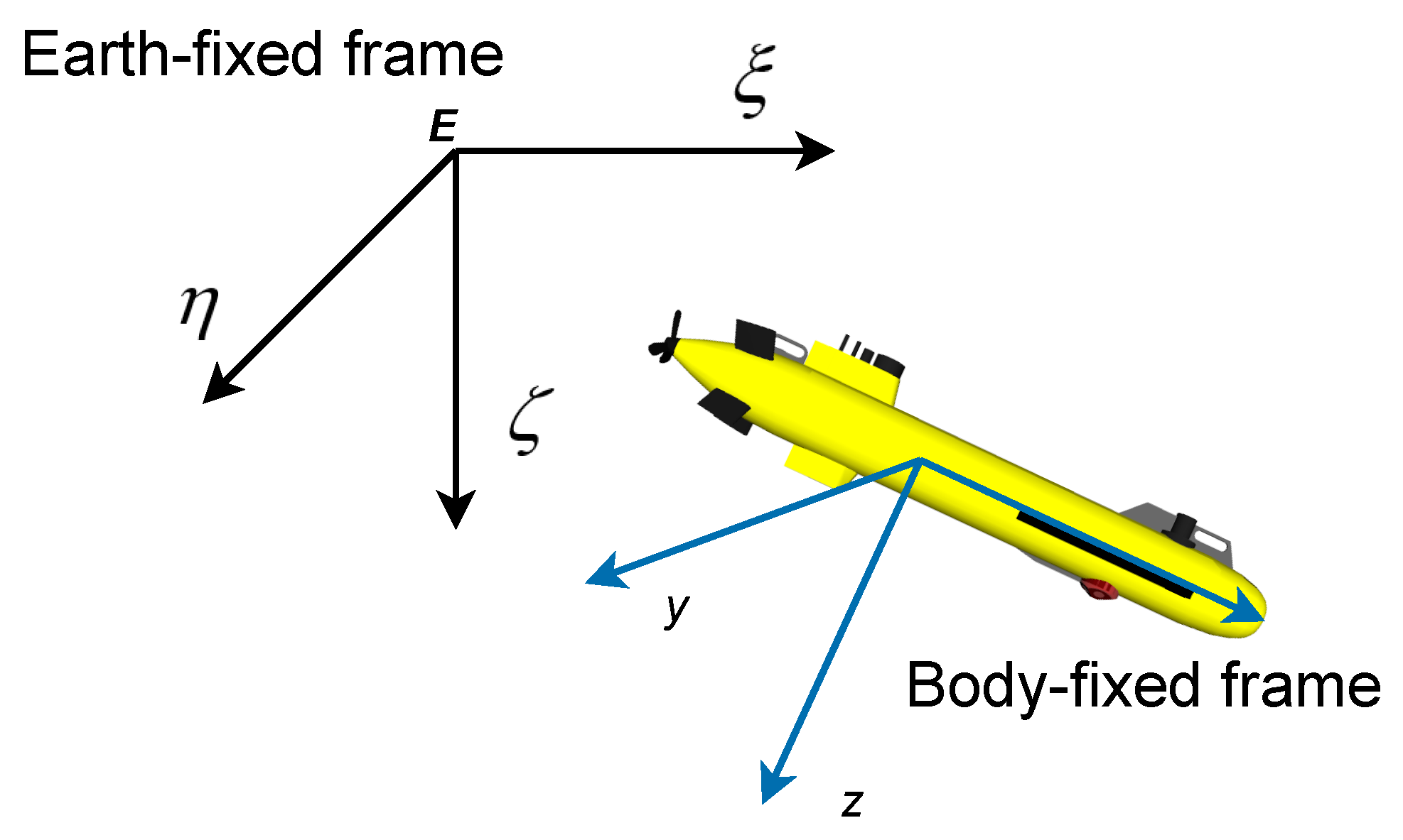
2.1.1. Coordinate Systems

When discussing issues related to AUV kinematics, the Earth-fixed frame ( E ξ η ζ ) is used as the inertial reference frame, with the center of the map space taken as the origin. The position and attitude of the AUV can be represented by the position vector of the Body-fixed frame ( o x y z ) relative to the Earth-fixed frame. The E ζ axis points to the geocenter in the positive direction, E η points to the geographical north, and E ξ points to the east (Figure 1).
Given that the research subject is an underactuated Autonomous Underwater Vehicle, the dynamic coupling between its degrees of freedom induced by underactuation necessitates that the generated trajectories account for the AUV’s maneuverability constraints. Specifically, the kinematic model incorporates saturation limits of translational and angular velocities and their interdependencies as critical constraints for path generation.
Regarding the roll axis, the axisymmetric underactuated AUV lacks direct control inputs. Owing to minimal environmental disturbances and the dominance of hydrostatic restoring moments, the roll motion exhibits negligible amplitude and can thus be disregarded in both modeling and trajectory planning [27].
The position and orientation of an underwater robot can be represented by the position vector of the origin of the body-fixed frame relative to the earth-fixed frame, where ( ξ , η , ζ ) denote the three components of the origin o of the body-fixed frame in the earth-fixed frame. The orientation vector ( θ , ψ ) consists of θ (pitch angle) and ψ (yaw angle). The transformation matrix R from the body-fixed frame to the earth-fixed frame is given by the following [8]:
R = R 1 0 3 × 2 0 2 × 3 R 2
Here, R is the transformation matrix from the body-fixed frame to the earth-fixed frame, where R 1 is the rotation matrix and R 2 is defined as follows:
R 1 = cos θ cos ψ sin ψ sin θ cos ψ cos θ sin ψ cos ψ sin θ sin ψ sin θ 0 cos θ
R 2 = 1 0 0 1 cos θ

2.1.2. Model of Motion

AUVs exhibit characteristics such as strong coupling, high nonlinearity, and high complexity during actual underwater navigation. Therefore, when considering AUV path planning, it is necessary to account for the mutual constraints among the five degrees of freedom to avoid generating paths that exceed the AUV’s maneuvering capabilities [28].
The mathematical model for 5-degree-of-freedom motion is as follows [29]:
p ˙ = R ( p i ) v i M ϖ i ˙ + C ( ϖ i ) ϖ i + D ϖ i + G ( η i ) = τ i
In the above equation, p i = [ ξ i , η i , ζ i , θ i , ψ i ] T is the pose vector of A i in the earth-fixed frame, where ξ i , η i , ζ i , θ i , and ψ i represent the north position, east position, vertical position, pitch angle, and yaw angle of A i , respectively; ϖ i = [ u i , v i , w i , q i , r i ] T is the velocity vector of A i in the body-fixed coordinate system, where u i , v i , w i , q i , and r i represent the surge velocity, sway velocity, heave velocity, pitch angular velocity, and yaw angular velocity of A i , respectively.
M = diag ( m 11 , m 22 , m 33 , m 44 , m 55 ) is the inertia matrix of the AUV, where the elements m j j ( j = 1 , 2 , , 5 ) are the mass and moment of inertia coefficients of the AUV. D = diag ( d 11 , d 22 , d 33 , d 44 , d 55 ) is the damping matrix of the AUV, where the elements d j j ( j = 1 , 2 , , 5 ) are the damping coefficients of the AUV.
C ( v ) is the Coriolis force matrix of the AUV, G ( η ) = [ 0 , 0 , 0 , Δ g G M L sin ( θ ) , 0 ] T is the restoring force matrix, where g G M L is the restoring moment coefficient of the AUV, Δ is the displacement, g is the gravitational acceleration, and M L is the metacentric height of the AUV.
τ i is the control force vector of A i . τ = [ X , Y , Z , M , N ] T = τ u + τ r + τ s represents the forces and moments applied to each degree of freedom of the underactuated AUV. Here, X, Y, and Z denote the surge, sway, and heave forces defined in the body-fixed frame O- x y z , respectively, while M and N denote the pitch and yaw moments in the body-fixed frame O- x y z . These include the thrust (moment) generated by the thrusters as well as the moments produced by the horizontal and steering rudders. The thrust (moment) τ u = [ X 1 , Y 1 , Z 1 , M 1 , N 1 ] T can be expressed as follows:
τ u = X 1 Y 1 Z 1 M 1 N 1 = T 0 0 0 0 = K T ρ n p 2 D p 4 0 0 0 0
where n p is the rotational speed of the thruster, D p is the propeller diameter, K T and K Q denote the thrust coefficient and torque coefficient, respectively. The moments generated by the steering rudder and horizontal rudder, τ r = [ X 2 , Y 2 , Z 2 , M 2 , N 2 ] T and τ s = [ X 3 , Y 3 , Z 3 , M 3 , N 3 ] T , can be expressed as follows:
τ r = X 2 Y 2 Z 2 M 2 N 2 = D R L R 0 0 x r L R = 0.5 C D R ρ A r u r 2 0.5 C L R ρ A r u r 2 0 0 0.5 x r C L R ρ A r u r 2
τ s = X 3 Y 3 Z 3 M 3 N 3 = D S 0 L S x r L S 0 = 0.5 C D S ρ A r u r 2 0 0.5 C L S ρ A r u r 2 0.5 x r C L S ρ A r u r 2 0
where L denotes the lift force of the rudder, D denotes the drag force, R and S represent the steering rudder and the horizontal rudder, respectively, x r is the distance between the rudder and the center of buoyancy of the underactuated AUV, ρ is the fluid density, A r is the surface area of the rudder, and u r is the relative velocity of the AUV in the fluid.
Due to the limitations of the AUV’s propeller rotational speed and the area of the steering rudder, the AUV is subject to constraints on its velocity and maneuverability during operation. These constraints include the coupling between the surge velocity and the angular velocity of the AUV. Such velocity constraints will serve as conditions in the subsequent path optimization process to ensure that the generated path conforms to the maneuvering capabilities of the AUV.

2.2. Ocean Current Modeling with Eddy

Autonomous underwater vehicles (AUVs) traveling underwater are subject to currents, which can lead to increased energy consumption and flight path deflection. Therefore, it is crucial to consider the ocean current factor when planning routes. In this paper, we consider spatially variable but time-constant currents that have different directions and strengths at different locations but remain constant in the time series.
Assuming that a bounded area containing known static obstacles is filled with ocean current fields of varying velocity, the AUV must navigate around the obstacles and adapt to the changing currents, ensuring safe arrival at the destination with minimal energy consumption. Equation (8) represents the mathematical model of a single viscous vortex field [30].
V ξ ( r ) = k c · η η 0 2 π ( r r 0 ) 2 1 e ( r r 0 ) 2 δ 2 V η ( r ) = k c · ξ ξ 0 2 π ( r r 0 ) 2 1 e ( r r 0 ) 2 δ 2 V ζ ( r ) = k c π δ 2 · e ( r r 0 ) 2 δ 2
where V ξ ( r ) , V η ( r ) , and V ζ ( r ) represent the speed in the longitude, latitude, and depth directions, respectively. Therefore, the ocean current vector at each position can be expressed as V ( r ) = V ξ ( r ) , V η ( r ) , V ζ ( r ) , where r 0 is the position vector of the vortex center, k c is the vortex radius, and δ is the eddy current strength. In this work, the actual motion vector of the AUV is considered as the combined effect of the AUV’s velocity in still water and the ocean current vector.
Multiple eddies acting together can simulate the complex ocean current environment. As shown in Figure 2, the situation of ocean currents under the combined action of three eddies is simulated.

3. Path Planning Method Based on Equal-Time Waypoint

During the navigation of an AUV, the propeller at its tail generates a backward wake, which can interfere with the navigation of other AUVs. Therefore, when designing paths for multiple AUVs, it is necessary to ensure that there is no conflict between any two AUVs. Motion conflicts between AUVs occur only when the distance between two AUVs is below the danger distance at the same time point. Even if two AUV paths have completely overlapping segments, as long as the two AUVs travel in a queue one after the other and maintain a distance greater than the danger distance, no conflict will occur.
To address the issue of multirobot conflicts, it is essential to obtain the path position information of each robot at different time points. Therefore, we have innovatively introduced the concept of equal-time waypoint.

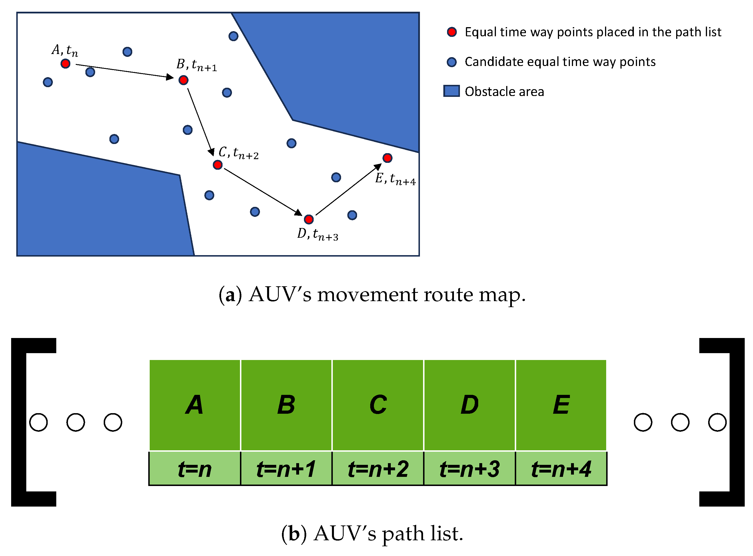
3.1. Equal-Time Waypoint

The concept of equal-time waypoint is based on the adaptive intermediate node insertion method [15] and the optimal path time planning (OPTP) method [31]. Both simplify continuous paths into multiple discrete nodes and solve the optimization problem through interpolation.
The equal-time waypoint method means that the time required for the AUV to travel between two adjacent equal-time waypoints in the path list is the same. When the AUV starts traveling, it first departs from the starting point and travels in a straight line to the position of the first equal-time waypoint in the path list. Then, it travels in a straight line to the next equal-time waypoint in the path list in sequence until it reaches the last equal-time waypoint and finally travels in a straight line to the destination. The time required for the AUV to travel between two adjacent equal-time waypoints in the path list is the same, which is the equal-time interval t i n t e r . Starting from the initial point, the AUV will reach the next equal-time waypoint at each fixed time interval t i n t e r until it reaches the destination. Therefore, a path list composed of equal-time waypoints corresponding to each AUV can represent both the path of the AUV and the time required to reach each position point. Since the distance between two adjacent equal-time waypoints is different, the time the AUV takes to travel between two adjacent equal-time waypoints is the same, and the running speed of the AUV on the segment between adjacent equal-time waypoints can be calculated.
For example, for an AUV ( A i ) with a path list of equal time waypoints P i = p i 1 , p i 2 , p i 3 p i n , the position coordinates of each equal time waypoint p i t in free space are p i t = ( ξ i t , η i t , ζ i t ) , where t < n . The next adjacent equal time waypoint is p i t + 1 = ( ξ i t + 1 , η i t + 1 , ζ i t + 1 ) . Therefore, we can calculate the speed of ϖ i t of the AUV on segment ( p i t , p i t + 1 ) via Equation (9).
ϖ i t = ( ξ i t + 1 ξ j t ) 2 + ( η i t + 1 η j t ) 2 + ( ζ i t + 1 ζ j t ) 2 t i n t e r
Since the travel time between two waypoints is the same, the greater the Euclidean distance between two equal-time waypoints is, the faster the AUV travels on segment l i t . In this way, when two adjacent equal time waypoints in the path list are the same equal time waypoint, A i remains stationary for the time interval t i n t e r starting from the time point t.
The generation of equal-time waypoints is based on the probabilistic road maps (PRM) method [32]. In the free space of a given graph, points P c a n d are randomly scattered. These points are referred to as landmarks in the PRM method, but in this paper, they serve as candidates for equal-time waypoints. The actual equal-time waypoints used are selected from these candidates and arranged in sequence to form a path list. A list composed of multiple equal-time waypoints represents the action path of each AUV (Figure 3).

3.2. Optimization of Path List

The initial path list generated via the above random method still needs further optimization. This paper proposes a path list optimization method based on four modules: delete, replace, exchange, and add. All four modules play important roles in the path optimization process.

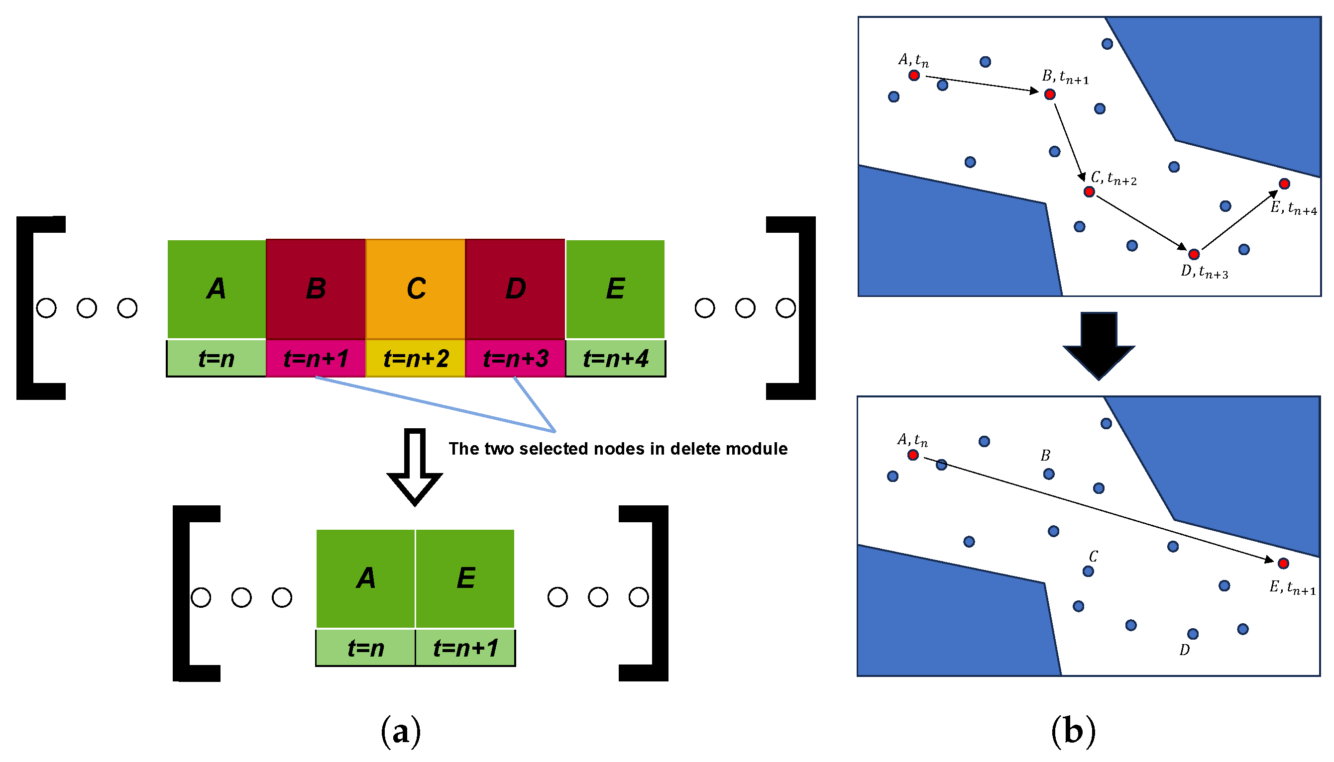
3.2.1. Delete Module

The delete operation aims to retain the useful parts of the path list. First, two elements in the list are randomly selected, and these two elements, along with the elements in between, are all deleted from the list, leaving the remaining parts to be concatenated into a new list. In practice, the delete module is divided into two modes, A and B, each of which plays a different role in path optimization.
In mode A, the newly formed list does not consider changes in the fitness function and directly checks that the new path is not blocked by obstacles. The delete operation in mode A does not necessarily improve the fitness function of the path list, which may lead to nonconvergence. However, this mode has an excellent ability to escape local optima.
In mode B, the algorithm evaluates the fitness of the newly generated path and compares the fitness value of the new path with that of the original path. If the new path shows lower fitness, it will replace the original list. Otherwise, the original list is retained. Mode B is a necessary operation to ensure the convergence of the algorithm. Figure 4 shows the working principle of the delete module.

3.2.2. Replace Module

The replace module performs replacement operations on elements in the path list with other candidate equal-time waypoints. A candidate equal-time waypoint is randomly selected and replaced with a randomly selected equal-time waypoint in the list, forming a new list.
Then, it checks whether the new path will cause conflicts and whether the straight-line connections formed between the new equal-time waypoint after replacement are blocked by obstacles. If there is an obstruction, the original list is retained.
Finally, the fitness of the new path is calculated. If the objective function of the new list is lower than that of the original list, the newly generated list will replace the original list; otherwise, the original list is retained. Figure 5 shows the working principle of the replace module.

3.2.3. Exchange Module
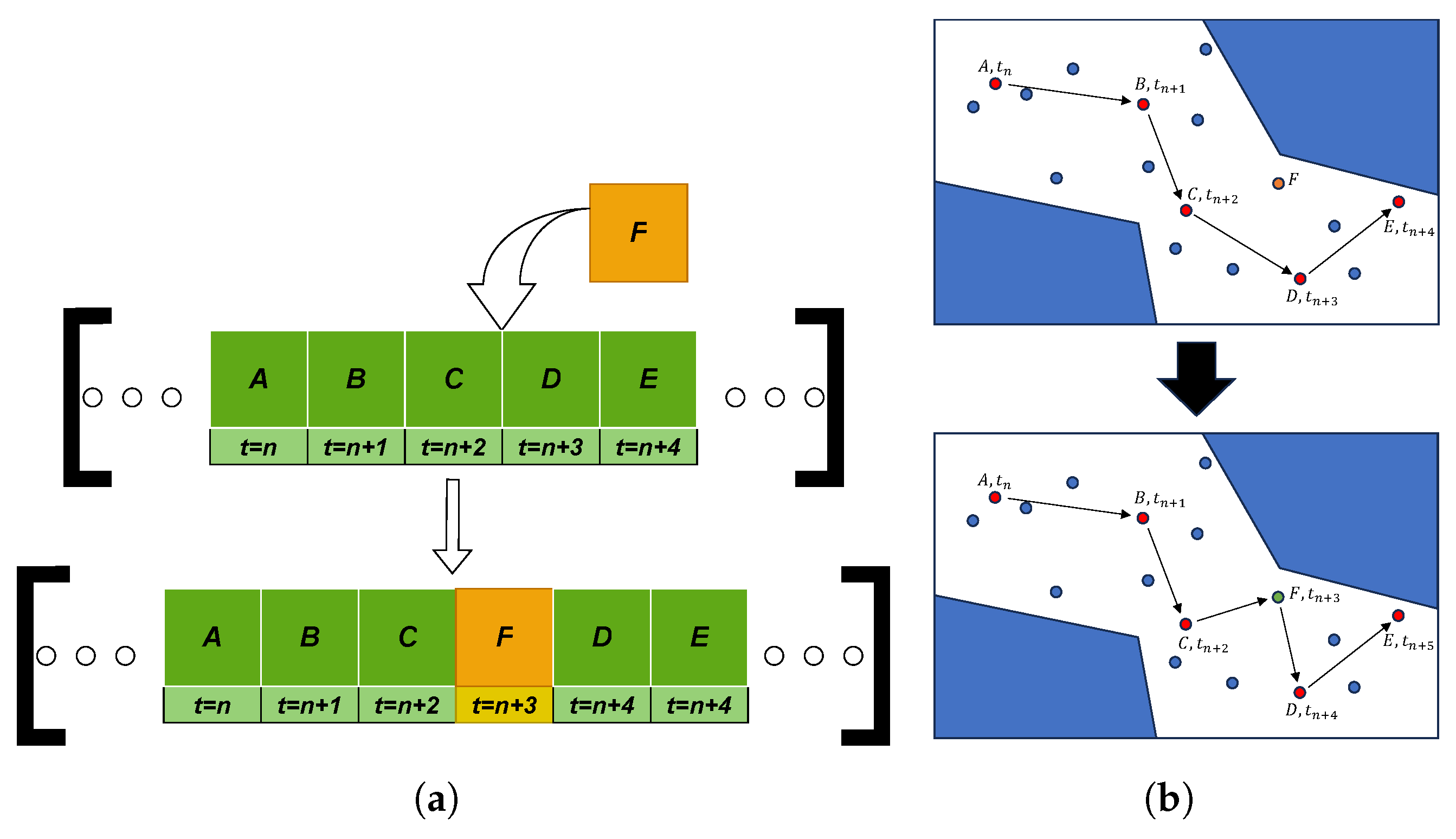
The order of equal-time waypoints in the path list also has a significant effect on fitness. Therefore, the exchange operation is used to obtain a better arrangement of equal-time waypoints.
In the exchange module, two equal-time waypoints in the list are randomly selected, and their positions are swapped. Then, it checks whether the new path list obtained after the exchange operation has any path obstructions. After confirming that there are no obstacles, the fitness value of the new path needs to be calculated to determine whether it has decreased compared with the original path. If there is an improvement, the new list will replace the original list; otherwise, the original list is retained.
The exchange operation, in conjunction with other operations, plays a decisive role in the convergence of the algorithm. Figure 6 shows the working principle of the exchange module.

3.2.4. Add Module

The add operation ensures that the number of elements in the path list remains at a reasonable level.
In the add module, a candidate equal-time waypoint is randomly selected from the set of candidate waypoints and randomly inserted into any position in the path list. Subsequently, it checks whether the new list is obstructed by obstacles.
If there are no obstructions, the fitness value of the new path list is calculated. If the fitness value of the new list decreases compared with that of the original list, the new list will replace the original path list; otherwise, the original path list is retained, and subsequent operations are performed. Figure 7 shows the working principle of the add module.

3.3. Objective Function

To ensure that the generated paths have low energy consumption and that there are no path conflicts between multiple AUVs, we design an objective function on the basis of the total path length, AUV speed variation, path smoothness, degree of ocean current influence, and multi-AUV collision risk coefficient. This objective function is used to evaluate the quality of the path list and optimize the path list on the basis of the fitness function.

3.3.1. The Total Path Length

For any AUV A i , there exists a path P i . Therefore, the set of paths for all AUVs is P = P 1 , P 2 , P 3 P n (where n is the total number of AUVs). Each path P i ( i n ) consists of several equal time waypoints, as well as a starting point and an endpoint. The number of equal time waypoints is determined by the actual situation. Thus, P i = p i 1 , p i 2 , p i 3 p i m , where p i k ( k m ) represents the position of the waypoint in free space such as p i k = ( ξ i k , η i k , ζ i k ) . For each path P i , p i 1 is the starting point of the AUV, and the last equal-time waypoint in the path, p i m is the endpoint of the path. Here, l i t represents the distance between the t-th equal-time waypoint and the ( t 1 ) -th equal-time waypoint in path P i of the i-th AUV. The objective function f t based on the total path length can be expressed as Equation (10).
l i t = ( ξ i t ξ i t 1 ) 2 + ( η i t η i t 1 ) 2 + ( ζ i t ζ i t 1 ) 2 f l = i = 1 n m a x t = 2 t m a x i l i t
where n m a x is the total number of AUVs, t m a x i is the number of equal time waypoints in path P i , and l i t is the distance between the t-th and ( t 1 ) -th equal time waypoints in path P i .

3.3.2. Influence of Ocean Currents on Paths

The direction and magnitude of ocean currents affect the movement of AUVs. When the movement of the AUV aligns with the direction of the ocean current, it can achieve energy savings. Conversely, when the movement of the AUV significantly differs from the direction of the ocean current, it can result in substantial energy loss.
Here, the vector V i t represents the velocity of the ocean current on the segment between p i t 1 and p i t . By Equation (11), the calculated vector l i t represents the path vector on the segment between p i t 1 and p i t , and the objective function f t based on the ocean currents can be expressed as Equation (12).
In practice, the ocean current velocity varies with position along the segment from p i t 1 to p i t . For computational convenience, the ocean current vector V i t is approximated by the current velocity at the midpoint of this segment.
l i t = p i t p i t 1
The relationship between the generated path and the ocean current is evaluated using the objective function defined in Equation (12).
f t = i = 1 n max t = 2 t max i V i t cos θ i t
where θ i t denotes the angle between the ocean current vector V i t and the path segment vector l i t at time t for the i-th AUV. The term cos θ i t measures the alignment between the ocean current and the path direction: a value of 1 indicates that the current is in the same direction as the path (assisting motion), 1 indicates the opposite direction (hindering motion), and 0 indicates that the current is perpendicular to the path.

3.3.3. Speed Offset

Since the movement speed of the AUV varies with different paths in this method, in practical operations, the movement speed of the AUV should neither be too fast nor too slow. If the AUV moves too fast, it needs to overcome more water resistance, increasing energy consumption. On the other hand, if the AUV moves too slowly, the time required to complete the total journey will be extended, increasing energy losses from AUV control equipment and sensors.
Without considering conflicts between AUVs, the AUV needs to maintain an optimal operating speed v b e s t . By the optimal operating speed and equal time interval, a reference equal time waypoint interval l r e f e r can be obtained via Equation (13).
l r e f e r = ϖ b e s t · t i n t e r
In the equal-time waypoint method, the speed of the AUV must change at different times to avoid mutual conflicts during movement. However, the AUV still needs to maintain the optimal operating speed as much as possible. By comparing the interval between equal-time waypoints in the path list with the reference equal time waypoint interval, the objective function f v can be obtained via Equation (14), where c o v e r and c b e l o w are the over-speed-loss factor and below-speed-loss factor, respectively.
f v = i = 1 n m a x t = 2 t m a x i ( l i t l r e f e r ) 2 · c o v e r , l i t > l r e f e r l r e f e r l i t · c b e l o w , l i t l r e f e r

3.3.4. Smoothness of the Path

Considering that AUVs incur more energy loss during turning operations than they do during straight-line travel, the actual AUV path planning process should minimize turning operations as much as possible. To increase the smoothness and continuity of the AUV path, the objective function, which is based on path smoothness, can be calculated via the direction vectors of the AUV on different segments. The objective function f s based on path smoothness can be calculated via Equation (15).
f s = i = 1 n m a x t = 2 t m a x i l i t 1 · l i t l i t 1 · l i t
The smoothness objective function is obtained by summing the negative cosine values of the angles between two adjacent segments. The value of the objective function decreases as the movement directions of two adjacent path segments become more similar.

3.3.5. Multiple AUV Collisions

To ensure that multiple AUVs do not approach each other within an unsafe distance at the same time node, their movement paths must maintain a distance greater than the safety threshold at the same time point. We use the axis-aligned bounding box (AABB) method to calculate the distance between each pair of AUVs at the same time point [33]. AABB is a simple bounding volume commonly used in computer graphics and physical simulations. By considering the equal-time waypoint coordinates of each AUV at the same time point, we can obtain the minimum distance c i , j t between AUVs on that segment with a relatively low computational cost via Equation (16).
D m i n i , j , t = min ξ i t , ξ i t + 1 , ξ j t , ξ j t + 1 , η i t , η i t + 1 , η j t , η j t + 1 , ζ i t , ζ i t + 1 , ζ j t , ζ j t + 1 , t t m a x 1 D m a x i , j , t = max ξ i t , ξ i t + 1 , ξ j t , ξ j t + 1 , η i t , η i t + 1 , η j t , η j t + 1 , ζ i t , ζ i t + 1 , ζ j t , ζ j t + 1 , t t m a x 1 c i , j t = D m i n i , j , t + D m a x i , j , t 2
Here, i and j represent the path lists of different AUVs, t denotes the t-th element in the path list. ξ , η and ζ are the horizontal and vertical coordinates of the waypoint, respectively.
The objective function f p , which is based on the collisions of AUVs, is described by Equation (17). When the distance between the movement paths of any two AUVs during the same time period is less than the safety distance c s a f e , a large penalty function is generated. In practice, we set this penalty to a sufficiently large numeric value, and our experiments show that the results are not sensitive to the specific value chosen, as long as it is large enough. If there is no possibility of collision on any segment for the AUVs, the collision penalty will not affect the objective function.
f p = + 100 , c i , j t < c s a f e ( 0 < t < t m a x , 0 < i < n m a x , 0 < j < n m a x , i j ) 0 , e l s e

3.3.6. Fitness Function

To guide the path search process of each AUV in a better direction, the total fitness function F can be summarized from the aforementioned objective functions, resulting in Equation (18).
F = c 1 · f l + c 2 · f t + c 3 · f v + c 4 · f s + f p
The parameters c 1 , c 2 , c 3 and c 4 represent the contribution of each penalty function branch and can be adjusted according to the actual situation. For example, to increase the smoothness of the AUV, the parameter c 4 of the smoothness penalty factor f s can be increased accordingly. During the optimization process, the kinematic constraints of the underactuated AUV described in Section 2.1.2, together with the maximum propeller rotational speed and the maximum effective area of the rudder, are incorporated as constraint conditions for optimization.

3.4. Multi-AUV Path Planning Method Based on Equal-Time Waypoint

The four modules work together to provide a good ability to escape local optima and achieve good convergence. The path list optimization method based on these four modules can be summarized in the following steps:
For each AUV, first generate an initial path list via the RPM-based method. For each initial path list, iterative path optimization operations are performed.
First, an AUV is selected, and operations are performed on its path list in the order of delete, replace, exchange, and add. The next AUV is selected, and the delete, replace, exchange, and add operations are repeated. The cycle is repeated until all AUVs have been processed.
For the choice between mode A and mode B in the delete operation, since the delete operation in mode A has a good ability to escape local optima, it is suitable for the early stages of optimization to find local optima. However, the delete operation in mode A can lead to nonconvergence of the algorithm. Therefore, after a good local optimum is found, the delete operation in mode A needs to be switched to mode B.
This method refers to the simulated annealing method, which controls the operation mode of the delete module by gradually lowering the temperature [34]. When the number of iterations is below the threshold T r e f e r , the delete module operates in mode A; when the number of iterations is above the threshold T r e f e r , the delete module operates entirely in mode B.
As the iteration progresses, the fitness of each AUV’s path list continuously decreases. When the fitness decreases to a certain level and no further reduction is observed after multiple iterations, the optimization is terminated, and the iterative process is completed.
To ensure the smoothness of the path, Gaussian smoothing can be applied to the data in the path list at the end. Gaussian smoothing is a convolution operation based on the Gaussian function. It achieves the effect of smoothing the path by performing a weighted average on each equal-time waypoint and its neighbouring equal-time waypoints. The kernel function is given in Equation (19), where ξ and η are the horizontal and vertical coordinates of each equal-time waypoint, respectively, and σ is the standard deviation of the Gaussian function. In practice, the smoothed path generally satisfies the kinematic constraints. As for optimality, the value of the objective function does increase slightly after smoothing; however, this increase remains within an acceptable range. The overall process of the method is shown in Figure 8.
G ξ , η , σ = 1 2 π σ 2 e ξ 2 + η 2 2 σ 2

4. Simulation Results and Analysis

To verify the ability of the equal-time waypoint method to solve multi-AUV cooperative path planning in terms of energy consumption and path conflict issues, we simulate different multi-AUV working environments in a 1000 m * 1000 m square area. Different environments have different characteristics of ocean currents and obstacle distributions.
First, a simulation experiment was conducted without considering the effects of ocean currents; three AUVs started from positions close to each other and reached different endpoints. The coordinates of the starting points and destination for the three robots are shown in Table 1.
In this basic environment, the parameters of the equal-time waypoint method are shown in Table 2, and the simulation results are shown in Figure 9.
The equal-time waypoint method will choose a shorter path, with equal-time waypoints evenly distributed along each path, with intervals of approximately 30 m. This indicates that the three AUVs essentially do not need to change speed to avoid conflicts, thus ensuring movement at the optimal operating speed.
This simulation experiment demonstrates that the equal-time waypoint method performs well in general working environments and has good universality.

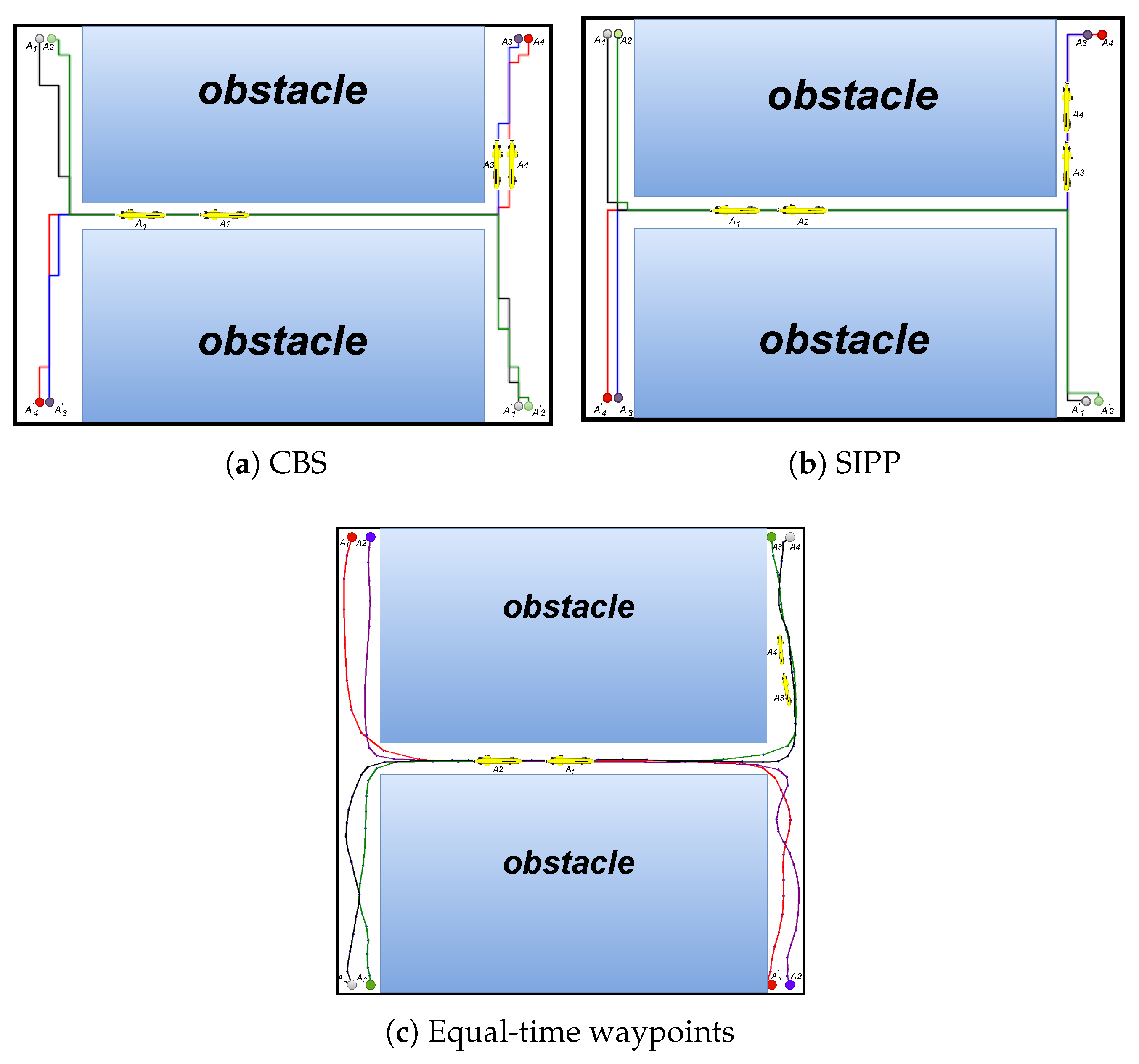
4.1. Comparative Experiments in Confined Spaces

To explore the ability of the equal-time waypoint method to solve path conflicts, we simulate an extreme scenario where four AUVs move in a map with a narrow track that allows only a single AUV to pass through at a time. Under these conditions, we verify the ability of the equal-time waypoint method to avoid conflicts in multiagent path planning.
In this map environment, the four AUVs start from A 1 , A 2 , A 3 , and A 4 , and their destinations are A 1 , A 2 , A 3 , and A 4 , respectively. The four AUVs need to navigate through narrow passages between obstacles to reach the destination areas on the other side. The narrow passage in the middle is set to allow only one AUV to pass through at a time. In this environment, the influence of ocean currents on AUV movement is not considered. The two-dimensional starting points and endpoints coordinates for the four AUVs, denoted as A 1 , A 2 , A 3 , and A 4 , are shown in Table 3.
We compare the equal-time waypoint method with the CBS method [5] and the SIPP method [4]. CBS (Conflict-Based Search) is a method where each agent is treated as an independent entity, aiming to find a feasible path to reach its target location while attempting to avoid conflicts with the paths of other agents. SIPP (Safe Interval Path Planning), on the other hand, is a single-agent planning algorithm that accounts for the trajectories of dynamic obstacles. In a multi-robot system, it prioritizes the robots and treats the trajectories of earlier planned robots as dynamic obstacle trajectories for the robots planned later. Both methods are utilized to resolve path conflicts in multi-robot path planning.
Figure 10a illustrates the process of the CBS method in addressing this issue, where A 1 and A 2 pass through a narrow channel while A 3 and A 4 wait side by side at the exit. As A 1 and A 2 are about to traverse the channel, A 3 and A 4 start from their waiting positions to pass through the channel.
Figure 10b shows that the results obtained via the SIPP method are similar to those of CBS. While A 1 and A 2 are navigating through the narrow channel, A 3 and A 4 queue up and wait at the exit of the narrow channel. Once A 1 and A 2 have passed through the channel, A 3 and A 4 immediately start queuing to pass through the narrow channel.
Figure 10c shows that the equal-time waypoints for A 1 and A 2 are more densely packed on the starting segment, whereas for A 3 and A 4 , the equal-time waypoints are more spread out on the starting path. In areas where equal-time waypoints are dense, the AUVs move more slowly, and when they are sparse, the AUVs move faster. On the basis of the information from the above figure, when the AUVs begin their operation, A 1 and A 2 start at a faster speed and quickly exit the narrow channel, whereas during the period when A 1 and A 2 are moving quickly, A 3 and A 4 move at a slower speed. As A 1 and A 2 are about to exit the channel, A 3 and A 4 just reach the entrance of the narrow channel. A 1 , A 2 , A 3 , and A 4 subsequently proceed to the endpoint at the reference speed.
In the CBS and SIPP methods, A 3 and A 4 of the AUV are required to stop and wait at the entrance of the narrow passage until A 1 and A 2 have passed through, after which they proceed to their destinations. However, for underactuated AUVs, especially in environments with ocean currents, it is difficult to maintain a completely stationary state. The motion degrees of freedom of the AUV are strongly coupled, making it challenging to control a single degree of freedom independently. Therefore, if disturbances such as ocean currents cause lateral drift during the waiting process, returning directly to the designated waiting position requires a series of complex maneuvers, which also significantly increases the risk of collision.
In contrast, in my method, A 3 and A 4 do not come to a complete stop, but instead move at a reduced speed, allowing them to avoid A 1 and A 2 as they traverse the narrow space. By maintaining motion, the new method can partially compensate for disturbances such as ocean currents.
Furthermore, due to the use of variable speed, my method offers a runtime advantage over the CBS and SIPP methods. Before a conflict occurs, the AUVs travel at speeds higher than the reference cruising speed, allowing them to quickly exit the conflict area. As a result, in the equal-time waypoint method, the travel times of A 1 and A 2 are only 61.7% and 65.6% of those in the previous two methods, respectively. The acceleration of A 1 and A 2 also enables A 3 and A 4 to enter the narrow passage more quickly, reducing their travel times to 67.5% and 69% of those in the previous methods, thus achieving the goal of time savings.

4.2. The Impact of Ocean Currents on AUV Paths

This section focuses on the impact of ocean currents on AUV paths. Theoretically, AUVs moving in the direction of ocean currents can achieve energy savings. In practice, simulation experiments have shown that the influence of ocean currents on AUV paths is quite limited, but AUVs do have the ability to save energy by moving in the direction of ocean currents, a conclusion also supported by previous research [35]. The specific effects of ocean currents on the proposed method can be observed in the selection of paths and certain changes in path details.

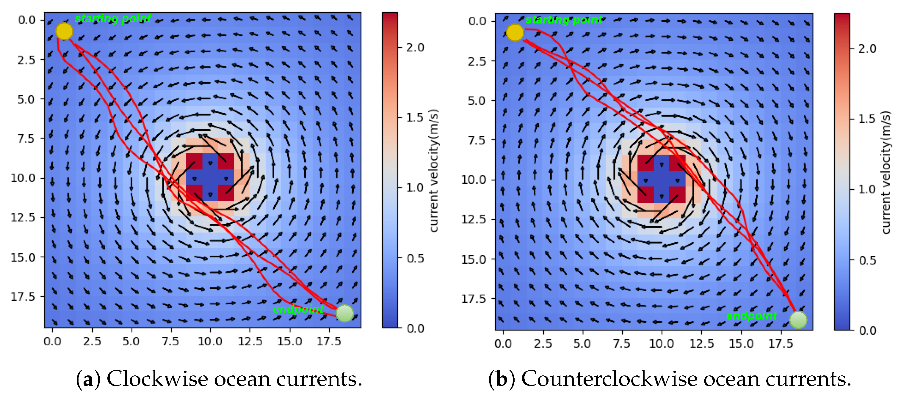
4.2.1. Selectivity of Ocean Currents on Paths

In a relatively open environment, there is an obstacle in the center of the map. Now, there is a vortex centered at the center of the map.
Three AUVs start from the upper left corner of the map and reach the lower right corner; their starting and ending coordinates are shown in Table 4. The cost of navigating around the obstacle (located near the center of the map) is the same, whether the AUVs choose to pass above it clockwise or counterclockwise. When the influence of ocean currents is taken into account, the AUVs will tend to move in the direction of the currents, similar to the path choice illustrated in Figure 11.
When the ocean current flows clockwise around the obstacle, the AUVs will correspondingly navigate around the obstacle in a clockwise direction. Conversely, if the ocean current flows counterclockwise around the obstacle, the AUVs follow the ocean current and navigate around the obstacle in a counterclockwise direction. In the equal-time waypoint method, ocean currents have a selective influence on AUV paths.

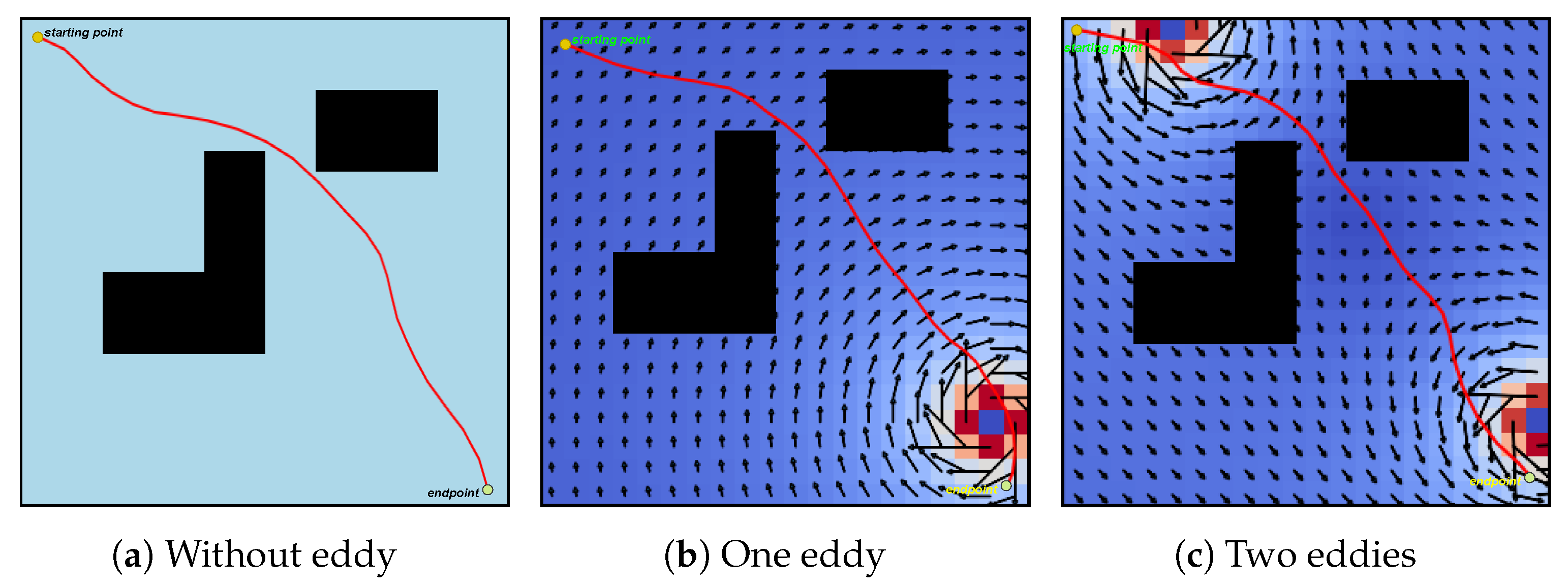
4.2.2. The Impact of Ocean Currents on Pathways

We simulate the path changes of a single AUV under conditions of no ocean current, a single vortex field, and a double vortex field. A single AUV starts from the top-left corner of the map and reaches the bottom-right corner. Without the influence of the ocean current, the AUV chooses a shorter path that avoids all obstacles and is sufficiently smooth. Next, we set up an eddy near the endpoint to observe the influence of the vortex on the AUV paths, and the AUV paths deviate due to the eddy. The AUVs move clockwise around the vortex. The same behavior can be observed in the influence of two eddies on the AUV; we set up two eddies near both the starting point and the endpoint of the AUVs. The vortex fields have a certain impact on the AUV paths. The specific situation can be found in Figure 12.
A comparative analysis was conducted to evaluate the fitness of current-agnostic paths versus current-aware paths in adapting to ocean current dynamics. Multiple experimental trials were performed to compute the minimum, mean, and variance of the fitness function, as summarized in Table 5.
The experimental results indicate that, in both the single-vortex and dual-vortex scenarios, the difference between the paths generated with and without current awareness is relatively small in the single-vortex environment. However, in the dual-vortex environment, there is a significant difference in the current adaptability function between the current-aware and current-agnostic paths. In this case, the paths generated with current awareness make greater use of the ocean currents, resulting in improved adaptability to the flow field.
Figure 13 presents a simulation-based evaluation of the energy-saving performance of vortex-aware path planning within the same vortical flow field. During the interval from 240 s to 300 s, corresponding to the period when the AUV traverses the vortex-affected region, the propeller rotational speed under the current-aware strategy was substantially lower than that of the current-agnostic path. Overall, the total propeller energy consumption was reduced by 4.8%, empirically demonstrating the energy-saving potential of vortex-adaptive path planning.

5. NMPC Control Simulation Results

AUV localization and velocity estimation capabilities need to be taken into account if the planning needs to modulate the vehicle’s velocity as a function of its position or proximity to obstacles.
The algorithm was simulated on the ROS platform, with a hardware platform equipped with an Intel Core i7-9750H@2.60 GHz CPU and 16G RAM. The simulation was conducted using the Gazebo platform, which has a realistic physics engine and a visualized simulation interface, with a simulation frequency of 10 Hz.
The simulation involved trajectory tracking of paths generated by the equal-time waypoint method to verify its effectiveness in avoiding conflicts. Trajectory tracking requires the AUV to follow a predefined path while accurately tracking a specific time-dependent curve.
To achieve good cooperation between the equal-time waypoint method and the NMPC controller, certain adaptations were made to the control method. Waypoints were interpolated using cubic spline interpolation to match the control cycle of the NMPC method.
First, using cubic spline interpolation, we insert the same number of waypoints between each pair of equal-time waypoints along the newly generated trajectory. To enhance control effectiveness, the number of interpolated waypoints between two adjacent equal-time waypoints should match the control horizon of the NMPC method. Specifically, the theoretical travel time of the AUV between two consecutive waypoints should equal the NMPC control cycle. This ensures that during the receding horizon optimization process, the newly generated waypoint list can roll forward synchronously with the control horizon. By coordinating the reference waypoints and travel times across different time intervals in this rolling manner, temporal errors in trajectory tracking are effectively managed.
A typical trajectory generated by the equal-time waypoint method was selected for simulation control experiments. This trajectory features frequent heading and speed variations, making it a representative case for validating the feasibility of the new approach.
From a purely trajectory perspective, the actual path demonstrates good conformity with the reference path (Figure 14). During the initial activation phase of the vehicle, significant discrepancies exist between the actual and reference trajectories, but these errors tend to stabilize over time. However, when the AUV undergoes substantial velocity changes, tracking errors increase. Generally, even under large error conditions, positional discrepancies on the x-axis and y-axis exhibit a complementary pattern; when one coordinate shows significant deviation, the other maintains relatively low error. In the absence of major disturbances, errors progressively diminish over time. Even at peak error instances, the positional discrepancy between actual and the mean Dynamic Time Warping (DTW) distance is less than 2.08 m, which remains within the acceptable range for equal-time waypoint methods.
It should be noted that the simplified model employed in this NMPC implementation differs from the actual AUV dynamics, introducing certain prediction inaccuracies. Additionally, considering the high computational demands of NMPC controllers, this simulation adopts a relatively long control horizon to ensure effective control under limited hardware capabilities. These factors collectively contribute to increased tracking errors. The proposed method is expected to exhibit improved performance in real-world implementations with optimized models and computational resources.

6. Conclusions and Future Work

This paper proposes a new solution to the problem of path conflicts in multi-AUV path planning. First, we innovatively introduce the concept of the equal-time waypoint, avoiding path conflicts between AUVs by controlling their speeds on different segments. The generated path list is then optimized through four modules: delete, replace, exchange, and add. An objective function is constructed on the basis of the path length, path smoothness, ocean current adaptability, and collision probability between AUVs for each AUV path list. Finally, the generated paths are smoothed via a Gaussian smoothing method, resulting in paths with good smoothness that effectively avoid collisions between AUVs through speed differences.
In the simulation experiments, the paths generated by the equal-time waypoint method showed selectivity toward ocean currents, and eddies had a certain impact on the AUV paths.
However, the equal-time waypoint method still has some shortcomings. Its computational time complexity increases with the number of agents, which may result in significant time consumption when handling large-scale multiagent path planning problems. Our future work will focus on reducing the algorithm’s complexity while enhancing the ability of the equal-time waypoint method to escape local optima. Additionally, we expand the workspace to more complex oceanographic conditions and add moving obstacles to simulate more complex AUV working environments.

Author Contributions

Conceptualization, C.Y. and K.S.; methodology, C.Y., K.S. and H.W.; investigation, C.Y. and K.S.; data curation, C.Y.; formal analysis, C.Y.; validation, C.Y.; visualization, C.Y.; writing—original draft preparation, C.Y.; writing—review and editing, K.S.; project administration, K.S. and H.W.; resources, K.S. and H.W.; supervision, K.S. and H.W.; software, H.W.; funding acquisition, H.W. All authors have read and agreed to the published version of the manuscript.

Funding

This research was funded by the National Natural Science Foundation of China under Grant No. 42206196.

Informed Consent Statement

Informed consent was obtained from all subjects involved in the study.

Data Availability Statement

The data presented in this study are available on request from the first author. The data are not publicly available due to privacy.

Conflicts of Interest

The authors declare no conflicts of interest.

References

  1. Sun, L.; Wang, Y.; Hui, X.; Ma, X.; Bai, X.; Tan, M. Underwater Robots and Key Technologies for Operation Control. Cyborg Bionic Syst. 2024, 5, 0089. [Google Scholar] [CrossRef] [PubMed]
  2. Wang, L.; Zhu, D.; Pang, W.; Zhang, Y. A survey of underwater search for multi-target using Multi-AUV: Task allocation, path planning, and formation control. Ocean. Eng. 2023, 278, 114393. [Google Scholar] [CrossRef]
  3. Gao, J.; Li, Y.; Li, X.; Yan, K.; Lin, K.; Wu, X. A review of graph-based multi-agent pathfinding solvers: From classical to beyond classical. Knowl.-Based Syst. 2024, 283, 111121. [Google Scholar] [CrossRef]
  4. Phillips, M.; Likhachev, M. SIPP: Safe interval path planning for dynamic environments. In Proceedings of the 2011 IEEE International Conference on Robotics and Automation, Shanghai, China, 9–13 May 2011; pp. 5628–5635. [Google Scholar] [CrossRef]
  5. Sharon, G.; Stern, R.; Felner, A.; Sturtevant, N.R. Conflict-based search for optimal multi-agent pathfinding. Artif. Intell. 2015, 219, 40–66. [Google Scholar] [CrossRef]
  6. Nazarahari, M.; Khanmirza, E.; Doostie, S. Multi-objective multi-robot path planning in continuous environment using an enhanced genetic algorithm. Expert Syst. Appl. 2019, 115, 106–120. [Google Scholar] [CrossRef]
  7. Qin, H.; Shao, S.; Wang, T.; Yu, X.; Jiang, Y.; Cao, Z. Review of Autonomous Path Planning Algorithms for Mobile Robots. Drones 2023, 7, 211. [Google Scholar] [CrossRef]
  8. Cheng, C.; Sha, Q.; He, B.; Li, G. Path planning and obstacle avoidance for AUV: A review. Ocean Eng. 2021, 235, 109355. [Google Scholar] [CrossRef]
  9. Zeng, Z.; Sammut, K.; Lian, L.; He, F.; Lammas, A.; Tang, Y. A comparison of optimization techniques for AUV path planning in environments with ocean currents. Robot. Auton. Syst. 2016, 82, 61–72. [Google Scholar] [CrossRef]
  10. Sun, B.; Zhu, D.; Tian, C.; Luo, C. Complete Coverage Autonomous Underwater Vehicles Path Planning Based on Glasius Bio-Inspired Neural Network Algorithm for Discrete and Centralized Programming. IEEE Trans. Cogn. Dev. Syst. 2019, 11, 73–84. [Google Scholar] [CrossRef]
  11. Zhu, D.; Zhou, B.; Yang, S.X. A Novel Algorithm of Multi-AUVs Task Assignment and Path Planning Based on Biologically Inspired Neural Network Map. IEEE Trans. Intell. Veh. 2021, 6, 333–342. [Google Scholar] [CrossRef]
  12. Chu, Z.; Wang, F.; Lei, T.; Luo, C. Path Planning Based on Deep Reinforcement Learning for Autonomous Underwater Vehicles Under Ocean Current Disturbance. IEEE Trans. Intell. Veh. 2023, 8, 108–120. [Google Scholar] [CrossRef]
  13. Wang, C.; Mei, D.; Wang, Y.; Yu, X.; Sun, W.; Wang, D.; Chen, J. Task allocation for Multi-AUV system: A review. Ocean Eng. 2022, 266, 112911. [Google Scholar] [CrossRef]
  14. Yin, L.; Yan, Z.; Tian, Q.; Li, H.; Xu, J. A novel robust algorithm for path planning of multiple autonomous underwater vehicles in the environment with ocean currents. Ocean Eng. 2024, 312, 119260. [Google Scholar] [CrossRef]
  15. Zhuang, Y.; Huang, H.; Sharma, S.; Xu, D.; Zhang, Q. Cooperative path planning of multiple autonomous underwater vehicles operating in dynamic ocean environment. ISA Trans. 2019, 94, 174–186. [Google Scholar] [CrossRef]
  16. Liu, X.F.; Fang, Y.; Zhan, Z.H.; Jiang, Y.L.; Zhang, J. A Cooperative Evolutionary Computation Algorithm for Dynamic Multiobjective Multi-AUV Path Planning. IEEE Trans. Ind. Inform. 2024, 20, 669–680. [Google Scholar] [CrossRef]
  17. Barer, M.; Sharon, G.; Stern, R.; Felner, A. Suboptimal variants of the conflict-based search algorithm for the multi-agent pathfinding problem. In Proceedings of the International Symposium on Combinatorial Search, Prague, Czech Republic, 15–17 August 2014; Volume 5, pp. 19–27. [Google Scholar]
  18. Li, J.; Ruml, W.; Koenig, S. EECBS: A Bounded-Suboptimal Search for Multi-Agent Path Finding. In Proceedings of the 35th AAAI Conference on Artificial Intelligence, AAAI 2021, Virtual, 2–9 February 2021; Volume 14A, pp. 12353–12362. [Google Scholar]
  19. Mei, Y.; Li, S.; Chen, C.; Han, A. A Multi-robot Task Allocation and Path Planning Method for Warehouse System. In Proceedings of the 2021 40th Chinese Control Conference (CCC), Shanghai, China, 26–28 July 2021; pp. 1911–1916. [Google Scholar] [CrossRef]
  20. Feng, S.; Zeng, L.; Liu, J.; Yang, Y.; Song, W. Multi-UAVs Collaborative Path Planning in the Cramped Environment. IEEE/CAA J. Autom. Sin. 2024, 11, 529–538. [Google Scholar] [CrossRef]
  21. Yakovlev, K.; Andreychuk, A.; Vorobyev, V. Prioritized Multi-agent Path Finding for Differential Drive Robots. In Proceedings of the 2019 European Conference on Mobile Robots (ECMR), Prague, Czech Republic, 4–6 September 2019; pp. 1–6. [Google Scholar] [CrossRef]
  22. García, E.; Villar, J.R.; Tan, Q.; Sedano, J.; Chira, C. An efficient multi-robot path planning solution using A* and coevolutionary algorithms. Integr. Comput.-Aided Eng. 2023, 30, 41–52. [Google Scholar] [CrossRef]
  23. Kumar, S.; Sikander, A. A novel hybrid framework for single and multi-robot path planning in a complex industrial environment. J. Intell. Manuf. 2024, 35, 587–612. [Google Scholar] [CrossRef]
  24. Sandström, R.; Uwacu, D.; Denny, J.; Amato, N.M. Topology-Guided Roadmap Construction with Dynamic Region Sampling. IEEE Robot. Autom. Lett. 2020, 5, 6161–6168. [Google Scholar] [CrossRef]
  25. Zhang, M.; Chen, H.; Cai, W. Hunting Task Allocation for Heterogeneous Multi-AUV Formation Target Hunting in IoUT: A Game Theoretic Approach. IEEE Internet Things J. 2024, 11, 9142–9152. [Google Scholar] [CrossRef]
  26. Xiong, M.; Xie, G. Swarm Game and Task Allocation for Autonomous Underwater Robots. J. Mar. Sci. Eng. 2023, 11, 148. [Google Scholar] [CrossRef]
  27. Li, J.H. 3D trajectory tracking of underactuated non-minimum phase underwater vehicles. Automatica 2023, 155, 111149. [Google Scholar] [CrossRef]
  28. Ebrahimpour, M.; Lungu, M. Finite-Time Path-Following Control of Underactuated AUVs with Actuator Limits Using Disturbance Observer-Based Backstepping Control. Drones 2025, 9, 70. [Google Scholar] [CrossRef]
  29. Patil, P.V.; Khan, M.K.; Korulla, M.; Nagarajan, V.; Sha, O.P. Design optimization of an AUV for performing depth control maneuver. Ocean Eng. 2022, 266, 112929. [Google Scholar] [CrossRef]
  30. Garau, B.; Alvarez, A.; Oliver, G. AUV navigation through turbulent ocean environments supported by onboard H-ADCP. In Proceedings of the 2006 IEEE International Conference on Robotics and Automation, 2006, ICRA 2006, Orlando, FL, USA, 15–19 May; 2006; pp. 3556–3561. [Google Scholar] [CrossRef]
  31. Zhang, C.; Li, Y.; Zhou, L. Optimal Path and Timetable Planning Method for Multi-Robot Optimal Trajectory. IEEE Robot. Autom. Lett. 2022, 7, 8130–8137. [Google Scholar] [CrossRef]
  32. Kavraki, L.; Svestka, P.; Latombe, J.C.; Overmars, M. Probabilistic roadmaps for path planning in high-dimensional configuration spaces. IEEE Trans. Robot. Autom. 1996, 12, 566–580. [Google Scholar] [CrossRef]
  33. Smith, A.; Kitamura, Y.; Takemura, H.; Kishino, F. A simple and efficient method for accurate collision detection among deformable polyhedral objects in arbitrary motion. In Proceedings of the Virtual Reality Annual International Symposium ’95, Research Triangle Park, NC, USA, 11–15 March 1995; pp. 136–145. [Google Scholar] [CrossRef]
  34. Romeo, F.; Sangiovanni-Vincentelli, A. A theoretical framework for simulated annealing. Algorithmica 1991, 6, 302–345. [Google Scholar] [CrossRef]
  35. Sun, B.; Niu, N. Multi-AUVs cooperative path planning in 3D underwater terrain and vortex environments based on improved multi-objective particle swarm optimization algorithm. Ocean Eng. 2024, 311, 118944. [Google Scholar] [CrossRef]
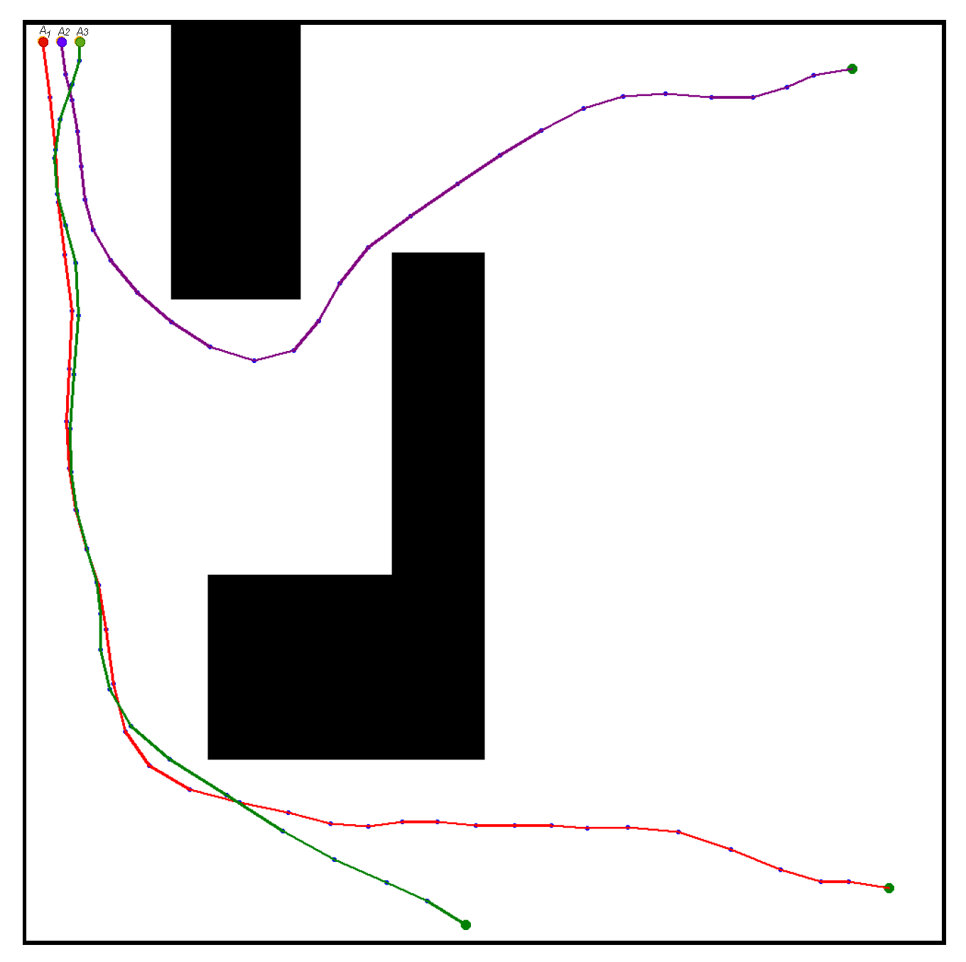
Figure 1. Earth-fixed frame and body-fixed frame.
Drones 09 00336 g001
Figure 2. Simulated the ocean current conditions under the combined influence of three eddies.
Drones 09 00336 g002
Figure 3. The relationship between the path list and the movement route.
Drones 09 00336 g003
Figure 4. Changes in the path list and AUV movement path under the delete module operation. (a) Changes in the path list under the delete module. (b) Changes in the path under the delete module.
Drones 09 00336 g004
Figure 5. Changes in the path list and AUV movement path under the replace module operation. (a) Changes in the path list under the replace module. (b) Changes in the path under the replace module.
Drones 09 00336 g005
Figure 6. Changes in the path list and AUV movement path under the exchange module operation. (a) Changes in the path list under the exchange module. (b) Changes in the path under the exchange module.
Drones 09 00336 g006
Figure 7. Changes in the path list and AUV movement path under the add module operation. (a) Changes in the path list under the add module. (b) Changes in the path under the exchange module.
Drones 09 00336 g007
Figure 8. Flowchart of the equal-time waypoint method for generating paths for multiple AUVs.
Drones 09 00336 g008
Figure 9. Simulation results showing the movement paths of three AUVs, with different colors representing the paths of different AUVs.
Drones 09 00336 g009
Figure 10. Path planning results of the equal-time waypoint method, CBS method, and SIPP method in narrow spaces.
Drones 09 00336 g010
Figure 11. Equal-time waypoint method has selectivity in path generation under both clockwise and counterclockwise ocean currents.
Drones 09 00336 g011
Figure 12. Differences in the paths of the equal-time waypoint method under varying numbers of eddies.
Drones 09 00336 g012
Figure 13. At approximately 240 s, the AUV enters the region affected by the eddy. Compared to the path generated without considering ocean currents, the path generated with current consideration results in lower propeller rotational speeds within the vortex-affected region.
Drones 09 00336 g013
Figure 14. Comparison of reference and actual trajectories in the simulation environment.
Drones 09 00336 g014
Table 1. Starting points and endpoints of multiple AUVs in a simulation experiment.
AUV NumberCoordinate of Starting PointCoordinate of Endpoint
A 1 (20, 20)(940, 940)
A 2 (40, 20)(900, 50)
A 3 (60, 20)(480, 980)
Table 2. Simulation experiment parameters for the equal-time waypoint method under a basic map.
SymbolParameterParameter Value
P c Number of random candidate equal-time waypoints1000
t inter Equal interval50 s
v best Optimal running speed1 m/s
c safe Safety distance5 m
T refer Temperature threshold3000
c over Over-speed-loss factor1
c below Below-speed-loss factor0.1
c 1 Path length influence factor1
c 2 Current influence factor2
c 3 Velocity offset influence factor1
c 4 Path smoothness influence factor1
σ Standard deviation of Gaussian function1
Table 3. Starting and ending coordinates of four AUVs in a confined space.
AUV NumberCoordinate of Starting PointCoordinate of Endpoint
A 1 (20, 20)(980, 980)
A 2 (40, 20)(960, 980)
A 3 (60, 20)(40, 980)
A 4 (60, 20)(20, 980)
Table 4. Starting and ending coordinates of three AUVs under the influence of a central vortex.
AUV NumberCoordinate of Starting PointCoordinate of Endpoint
A 1 (20, 20)(920, 920)
A 2 (40, 40)(940, 940)
A 3 (60, 60)(960, 960)
Table 5. Comparison of Fitness Function Metrics with and without Current Consideration.
Experimental ScenarioCurrent ConsiderationMeanMaxMinStd Dev
Single VortexWithout Current5.1311.95−5.354.92
With Current−3.782.46−11.785.07
Dual VorticesWithout Current−29.6295.27−99.3573.69
With Current−530.02−97.42−1888.01506.96
Disclaimer/Publisher’s Note: The statements, opinions and data contained in all publications are solely those of the individual author(s) and contributor(s) and not of MDPI and/or the editor(s). MDPI and/or the editor(s) disclaim responsibility for any injury to people or property resulting from any ideas, methods, instructions or products referred to in the content.

