High-Precision Landing on a Moving Platform Based on Drone Vision Using YOLO Algorithm

Abstract

High-precision landing is a key technical problem that Unmanned Aerial Vehicles (UAVs) will encounter in all application fields, especially for the landing of moving targets. This paper focuses on developing a landing system designed to achieve real-time precise navigation by integrating the Global Navigation Satellite System (GNSS) with the quadcopter’s vision data. To overcome the challenge of the flight altitude being too high to detect the landing target, this paper first detects large-volume targets, followed by the precise identification of smaller targets, achieving enhanced recognition accuracy and speed through an improved YOLOv8 OBB algorithm. To maintain the UAV’s safety and stability throughout the landing process, this paper applies a position control approach using a reference model-based sliding mode controller (RMSMC). The quadcopter’s position is then controlled by the RMSMC throughout the entire landing procedure. The reference value of each state is determined by the reference model, which improves the stability and safety of the entire position control system. During the final experiment, the results demonstrate that the enhanced YOLOv8 OBB identification model increases the mAP0.5:0.95 index for landing target point detection by 2.22 percentage points compared to the original YOLOv8 OBB model, running at 53 FPS on Nvidia AGX. Through multiple actual flights, the proposed landing system consistently achieves an average position error of just 0.07 m.

1. Introduction

With the advancement in quadcopter technology, quadcopters have quickly become a popular flying platform across various application fields. Their simple design, adaptability in control, and ability to perform vertical flight maneuvers have made them widely adopted. They are not limited only to traditional military reconnaissance and geographic mapping, but also play an important role in logistics and transportation, environmental monitoring, agricultural management, and emergency rescue [1,2,3]. However, due to the limitations of a quadcopter’s batteries, quadcopters cannot sustain prolonged flight and must land frequently. Ensuring a safe and stable landing in various conditions is thus a critical challenge in enhancing the autonomy of quadcopter missions. Particularly in dynamic environments, autonomously identifying and accurately locking onto a landing point without human intervention presents a significant challenge for quadcopter systems. Therefore, intelligent recognition systems and precise autonomous guidance strategies are crucial. They not only ensure the safety of quadcopter landings but also directly impact the success rate of the mission [4,5].

In the early days, many scientists used traditional guidance strategies based only on GNSS [6,7]. However, GNSS signals are often blocked or interfered with in complex or restricted environments, leading to significant positioning errors. As a result, GNSS alone cannot meet the requirements for the high-precision fixed-point landings of quadcopters. With the advancement in image recognition technology, vision-based and image processing techniques have gradually emerged, offering a more accurate and reliable solution. This approach improves the precision of quadcopter landings while minimizing dependence on external positioning systems, fostering the further development of autonomous quadcopter mission capabilities. Landing based on drone vision is usually affected by two factors: target recognition accuracy and landing control stability.

For target recognition, while traditional edge detection algorithms can identify the outlines of landing targets in simple environments, they have significant limitations in more complex environments. Edge detection algorithms are highly susceptible to changes in lighting, noise interference, and background complexity, which can lead to reduced target recognition accuracy [8,9,10]. Additionally, in our previous experiments, during high-altitude flight, the landing target appears too small in the field of view, making it challenging for the edge detection algorithm to identify it accurately [11]. In such cases, traditional edge recognition algorithms struggle to effectively identify larger secondary targets, such as dynamic objects like vehicles, and are unable to perform pre-tracking and positioning to assist with landing. Mainstream approaches are now categorized into one-stage and two-stage detection methods as a response to the rapid development of object detection technologies and the challenges in target recognition. First, the two-stage methods, for example, Faster R-CNN [12], offer high accuracy but are slow and computationally intensive. In contrast, one-stage methods, including well-known approaches like YOLO and SSD, significantly improve detection speed by integrating target positioning and classification tasks, making them particularly suited for real-time scenarios [13,14,15,16]. With advancements in algorithm and architecture optimization, YOLO’s accuracy has been significantly improved, even surpassing two-stage methods in some scenarios, making it the preferred solution for complex target detection tasks. Lee et al. developed a deep learning-driven solution for automatic landing area positioning and obstacle detection for quadcopters. However, this approach is susceptible to false detections due to perspective changes and the presence of obstacles [17]. Leijian Yu et al. integrated the improved SqueezeNet architecture into YOLO to detect landing landmarks and make it robust to different lighting conditions. However, it was not tested in dynamic and complex environments [18]. BY Suprapto et al. used Mean-Shift and Tiny YOLO VOC to detect falling targets, but the Mean-Shift method had a poor detection effect on moving objects and, although Tiny YOLO VOC had high detection speed and accuracy, its detection performance would decrease at higher altitudes [19]. Ying Xu et al. developed an advanced A-YOLOX algorithm, incorporating an attention mechanism to enhance the autonomous landing capabilities of quadcopters, particularly improving the recognition of small and mid-sized objects as well as adapting to varying lighting conditions. However, the article mentioned that the control algorithm still needs to be further optimized to enhance the safety of landing [20]. Tilemahos Mitroudas et al. compared the YOLOv7 and YOLOv8 algorithms in a quadcopter safe landing experiment and found that the performance improvement of YOLOv8 made detection and data more reliable [21]. Kanny Krizzy D. Serrano et al. compared four generations of algorithms from YOLOv5 to YOLOv8 to ensure the safe landing of quadcopters, and found that YOLOv8 achieved the highest average accuracy, outperforming other YOLO architecture models [22]. During the dynamic landing of UAVs, factors such as complex background environment, changes in lighting conditions, and local blur of targets will affect the accuracy of target recognition, and the difficulty in detecting small targets at high altitudes further exacerbates this challenge. Therefore, improving the performance of the recognition algorithm, enhancing the ability to extract key features, enabling UAVs to accurately focus on the target area under complex background conditions and improving the compatible detection capabilities of multi-scale targets are of great significance to improving the success rate in the stable landing of UAVs.

In conclusion, once the target is identified, it is essential to implement a controller that guarantees the stability throughout the landing procedure [20]. Lin et al. proposed a visual servo-based landing controller (PBVS) for landing on a mobile platform. The controller has low computational complexity and strong robustness, but it relies on the camera’s field of view and has high requirements for parameter adjustment [23]. Wu et al. proposed a RL-PID controller that can automatically adjust the PID parameters during the landing process, but its landing accuracy is greatly affected by environmental changes [24]. Alireza Mohammadi et al. employed the extended Kalman filter for position estimation using UAV vision, while utilizing an MPC controller to achieve dynamic landing. But, the calculation complexity was high and it was more dependent on the model [25]. In addition to the methods mentioned, various controllers like PID control [26,27], backstepping control [23,28], and adaptive control [29,30] have also been used for quadcopter landing. Among them, the sliding mode controller excels in dynamic landing due to its strong robustness and adaptability to uncertainty and disturbances. It can effectively handle environmental changes and uncertainties in system models [31,32,33], and therefore can help improve landing accuracy and stability during landing to a certain extent. Therefore, this paper selects a sliding mode controller to enhance the stability of the UAV in dealing with disturbances during landing.

Based on the previous discussion, to achieve the precise dynamic landing of quadcopters, the landing target detection system in this paper is built upon the advanced YOLOv8 OBB algorithm. Additionally, RMSMC is utilized during the landing process to ensure both stability and accuracy in landing control. The primary contributions of this paper include the following:

• To ensure precise positioning of the landing point, we enhanced the YOLOv8 OBB algorithm and deployed the optimized model on the quadcopter. By combining pixel error conversion with attitude angle compensation, we were able to obtain accurate distance errors, enabling the quadcopter to precisely identify the landing point. The accuracy and feasibility of this method were validated through experiments.
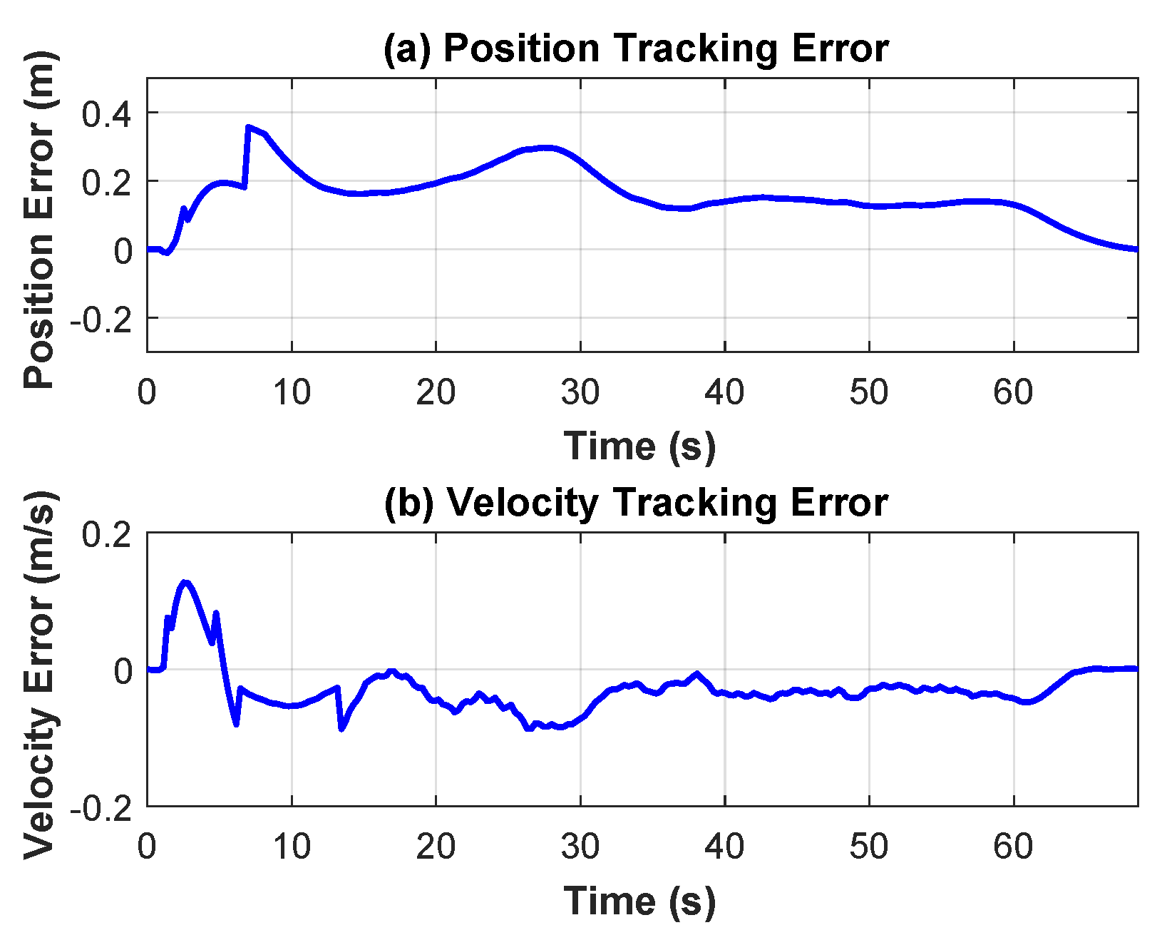
• The performance and accuracy of the landing system were verified through flight tests. The results show that the improved YOLOv8 OBB algorithm improves mAP@0.5 by 3.1% and mAP@0.5:0.95 by 2.61% on the VisDrone/DroneVehicle datasets, and mAP@0.5 by 0.5% and mAP@0.5:0.95 by 2.1% on private datasets, compared with the latest version of YOLOv8 OBB. In addition, when the proposed controller is deployed, the maximum position tracking error is kept within 0.23 m and the maximum landing error is kept within 0.12 m. The experimental video can be found at https://doi.org/10.6084/m9.figshare.28600868.v1 (accessed on 26 March 2025).

The structure of this paper is as follows: Section 2 and Section 3 provide an overview of the system architecture, including the design of the vision algorithm and controller. Section 4 describes the experimental setup and presents the results. Finally, Section 5 concludes the paper and outlines future work.

2. Visual Identification System Design

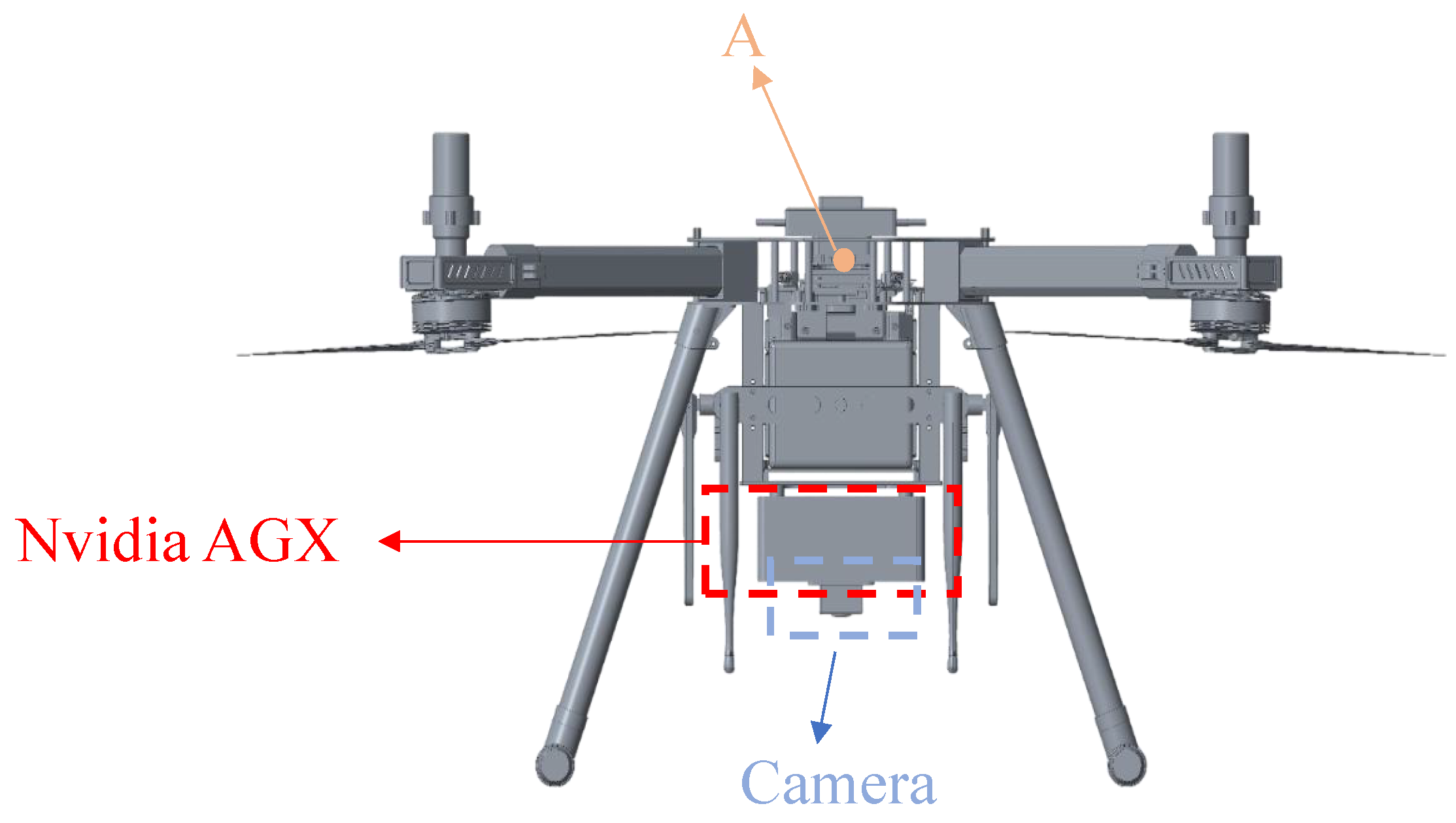
The quadcopter used in this system was independently developed by our team, as shown in Figure 1.

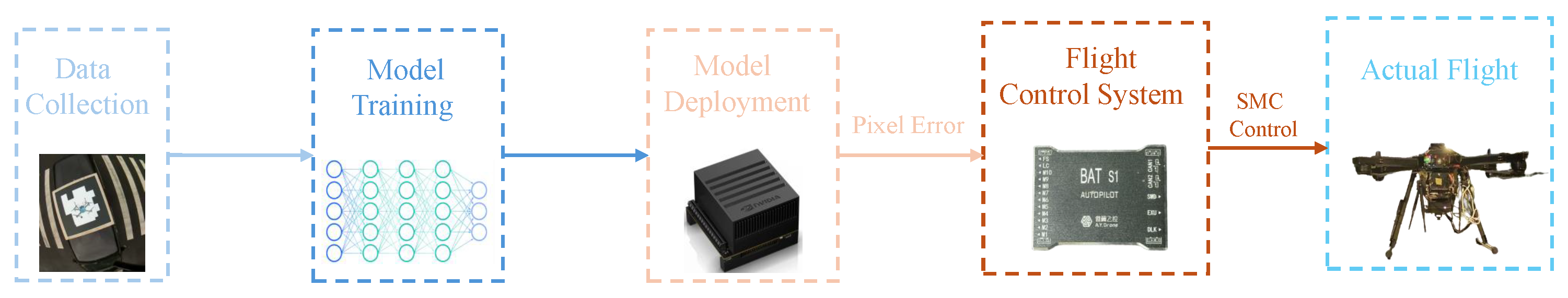
Figure 2 illustrates the system structure. First, quadcopters are used to collect the necessary experimental data. Then, the landing target recognition model is trained on an external computer before being deployed to the onboard Nvidia AGX platform. The overall system workflow is as follows: the image captured by the camera in real time is transmitted to the Nvidia AGX for recognition processing. Specifically, Nvidia AGX calculates the pixel error, converts it into the actual distance error based on the recognition results, and feeds this information back to the flight control system. Finally, the quadcopter adjusts its position using position and altitude control to ensure that the landing point remains centered beneath the quadcopter. The bottom layer of the system consists of the camera driver and quadcopter sensors. The framework layer includes open-source libraries such as Robot Operating System (ROS), PyTorch, and OpenCV. The application layer handles the flight control and dynamic landing of the quadcopter.

2.1. YOLOv8 OBB Algorithm

To improve landing adaptability, this paper adopts the YOLOv8 OBB algorithm, which incorporates the target’s rotation angle as part of the landing recognition process. YOLOv8 OBB integrates an oriented bounding box (OBB) mechanism into the YOLOv8 framework to enhance detection of objects with strong directional features. To enhance the input data, some advanced augmentation methods, including cropping accompanied by certain rotation operations, are applied, achieving a 3.1% accuracy improvement on the COCO dataset. During training, the model stabilizes learning by refining the data augmentation strategy in the final epochs, enabling efficient training from scratch without requiring pre-trained models. Structurally, YOLOv8 and YOLOv8 OBB share the same backbone (EfficientNet) and neck, which combines a feature pyramid network (FPN) with a spatial attention module (SAM).

YOLOv8 OBB builds upon YOLOv8 by modifying the output layer to include an oriented bounding box detection head, enhancing rotated object detection accuracy and speeding up convergence, albeit with slightly higher computational demands. To optimize performance and efficiency, it uses a 1 × 1 convolution in the output layer for dimensionality reduction and employs a 5 × 5 convolution in subsequent layers to control parameter expansion, ensuring high-precision detection is preserved.

2.2. Improved YOLOv8 OBB Algorithm

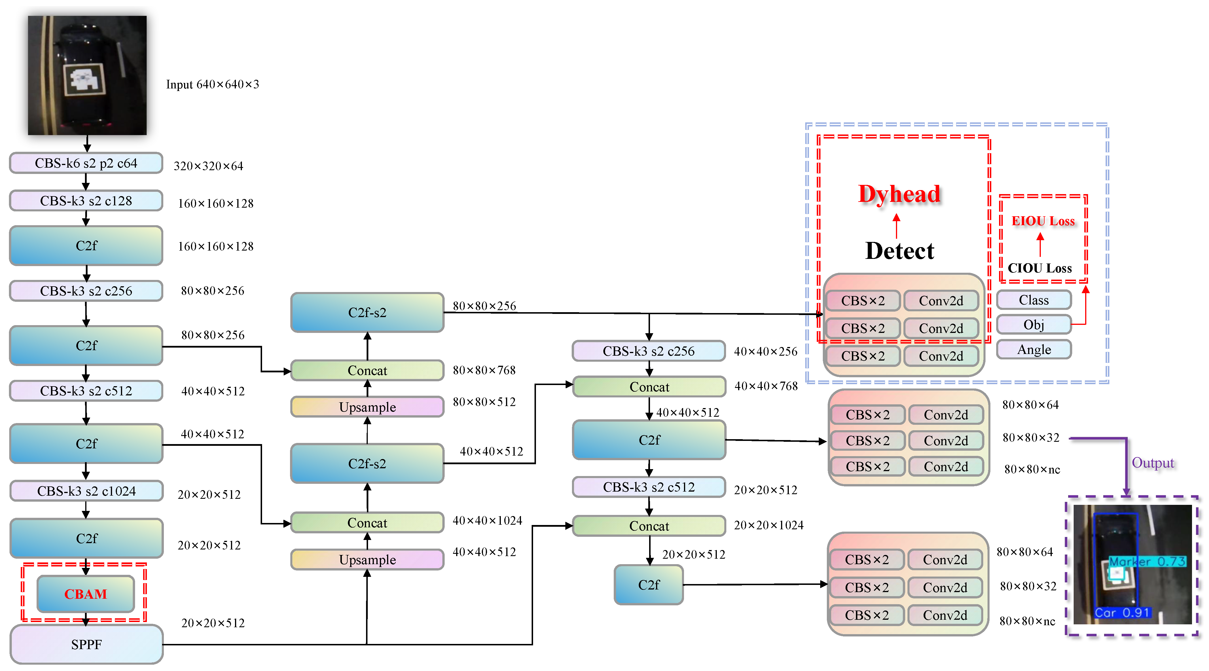
The accuracy of landing target recognition is crucial to ensure the safety and precision of the landing process. Factors such as complex backgrounds and lighting changes can significantly affect recognition performance, and the difficulty in detecting small targets at high flight altitudes further increases the challenge. To enhance recognition accuracy, this paper improves the baseline YOLOv8 OBB model by integrating three key components: the Convolutional Block Attention Module (CBAM) [34], Dyhead [35], and EIoU loss.

First, a CBAM is incorporated following the last layer of the backbone to capture spatial information while preserving precise positional data. This integration improves the model’s focus on critical areas within complex scenes, enabling accurate landings across diverse environments. Second, the Dyhead module is employed to dynamically refine feature representations across multiple scales and directions, enhancing the receptive field and robustness to objects of varying orientations and sizes. This further improves recognition accuracy and model stability. Additionally, in the dynamic quadcopter landing task, where large vehicles are identified before smaller landing spots, the original CIoU loss is replaced with EIoU loss. This adjustment enhances accuracy, ensuring the quadcopter reliably identifies landing targets even in challenging environments. Together, these modifications significantly improve detection performance, particularly in dense and directionally complex scenes. The improved YOLOv8 OBB structure is illustrated in Figure 3.

2.3. Convolutional Block Attention Module

In the realm of object detection, the attention module is commonly employed to improve the model’s ability to focus on important features, boosting both selectivity and sensitivity. Common attention mechanisms include compressed excitation network (SENet) [36], coordinated attention (CA) [37], efficient channel attention (ECA) [38], and CBAM [34]. SENet improves the importance of features by compressing feature maps along spatial dimensions using global average pooling to generate global descriptors, followed by a scaling step that amplifies key features and reduces the influence of less relevant ones. ECA improves the attention of the channel by replacing SENet’s fully connected layer with a 1 × 1 convolution, eliminating dimensionality reduction and reducing parameters while maintaining efficiency and accuracy. CBAM extends SENet by incorporating spatial attention alongside channel attention, enabling more precise feature processing. In the dynamic landing task, the integration of CBAM can significantly improve the recognition accuracy of vehicles and landing targets by adaptively refining feature representations through channel and spatial attention mechanisms [39]. The channel attention module prioritizes the most informative features by reweighting feature maps, while the spatial attention module focuses on key spatial regions to improve the detection of small targets or partially occluded targets. Moreover, its lightweight design minimizes computational overhead, making CBAM particularly suitable for resource-constrained UAV systems that require real-time processing. In addition, it can enhance feature discrimination capabilities under different lighting conditions and complex backgrounds to ensure robust performance, which is critical for the safety and reliability of UAV dynamic landing operations.

To improve recognition accuracy, CBAM optimizes convolutional neural networks for better recognition accuracy by leveraging both channel and spatial attention features. It first employs a channel attention module, using global average and maximum pooling to generate importance weights that emphasize critical features. Next, the spatial attention module processes the feature map using pooling followed by convolution operations, concentrating on key spatial regions.

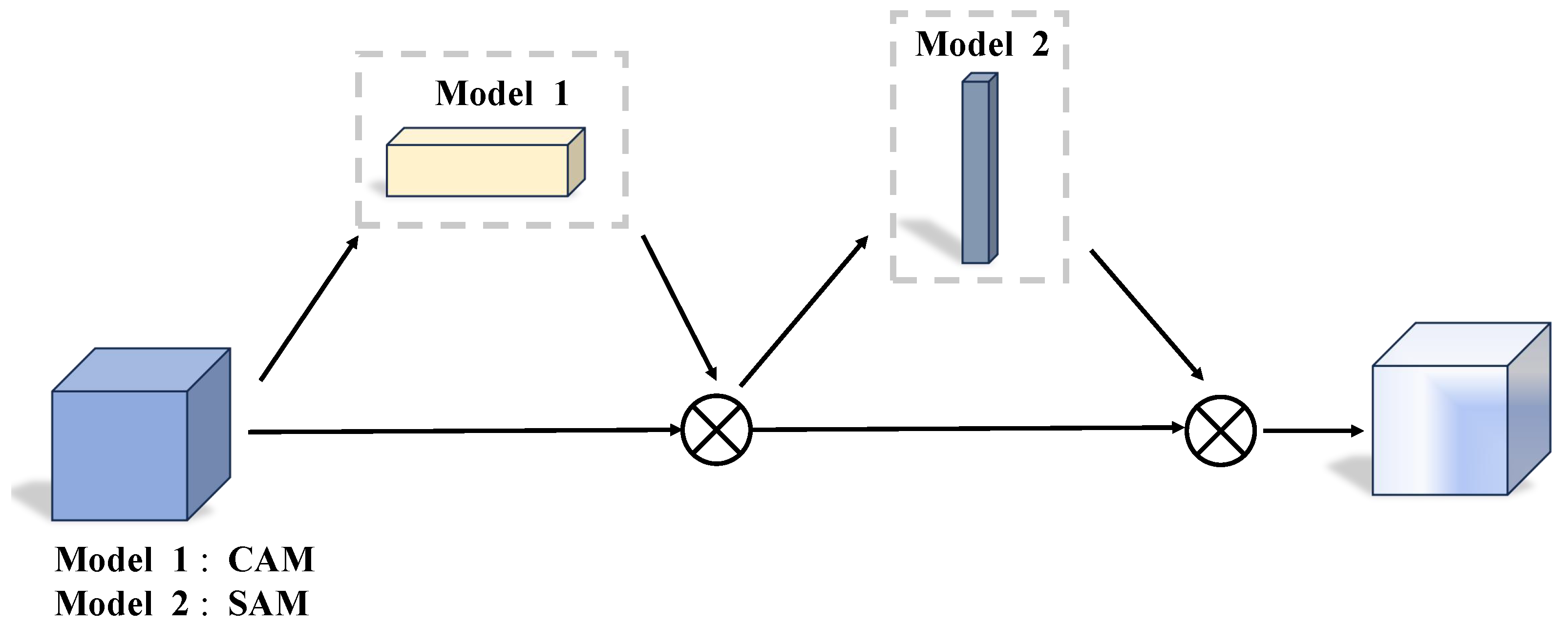
In summary, CBAM is made up of two parts: the channel attention module (CAM) and the spatial attention module (SAM), with their outputs fused through element-wise multiplication to generate the final result. The overall structure is shown in Figure 4:

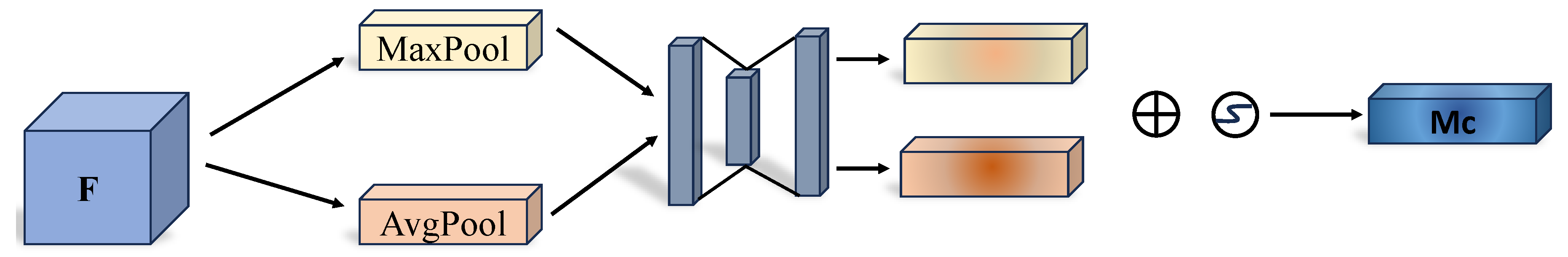
Figure 5 depicts the design of the channel attention module (CAM). The feature map F is first processed using both global average and maximum pooling operations. The pooled results are subsequently fed into a multi-layer perceptron (MLP) to generate the channel attention weights $M_C$. These weights are then applied to the original feature map F to emphasize the most relevant feature channels, and the final output is obtained by applying a sigmoid activation.

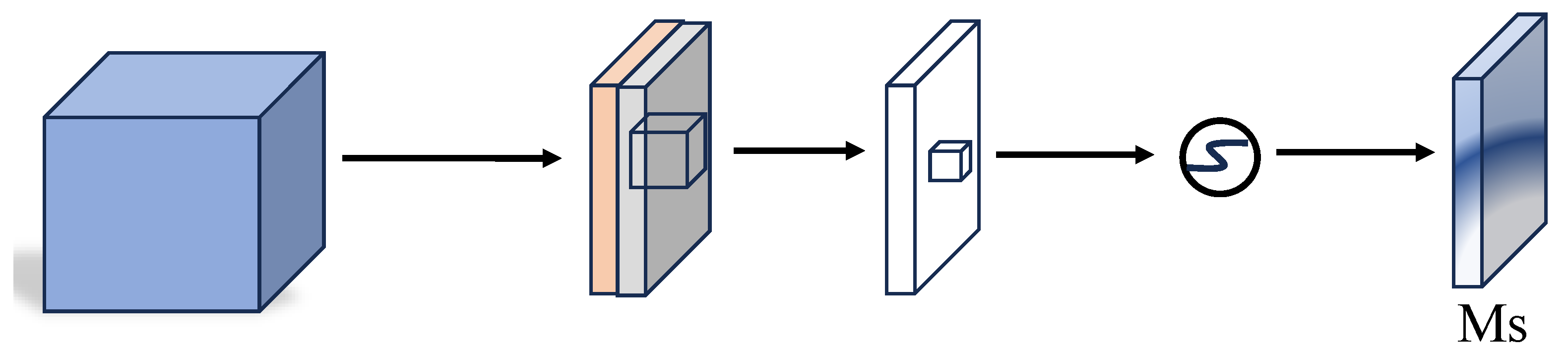
Figure 6 illustrates the design of the SAM. The module takes as input the feature map produced by the CAM, from which two separate feature maps are generated using global maximum and average pooling operations to capture spatial importance. These pooled maps are then concatenated along the channel axis and passed through a convolutional layer to compute the spatial attention map $M_S$. This attention map is then element-wise multiplied with the input feature map, producing the final output of the SAM.

2.4. Dynamic Head

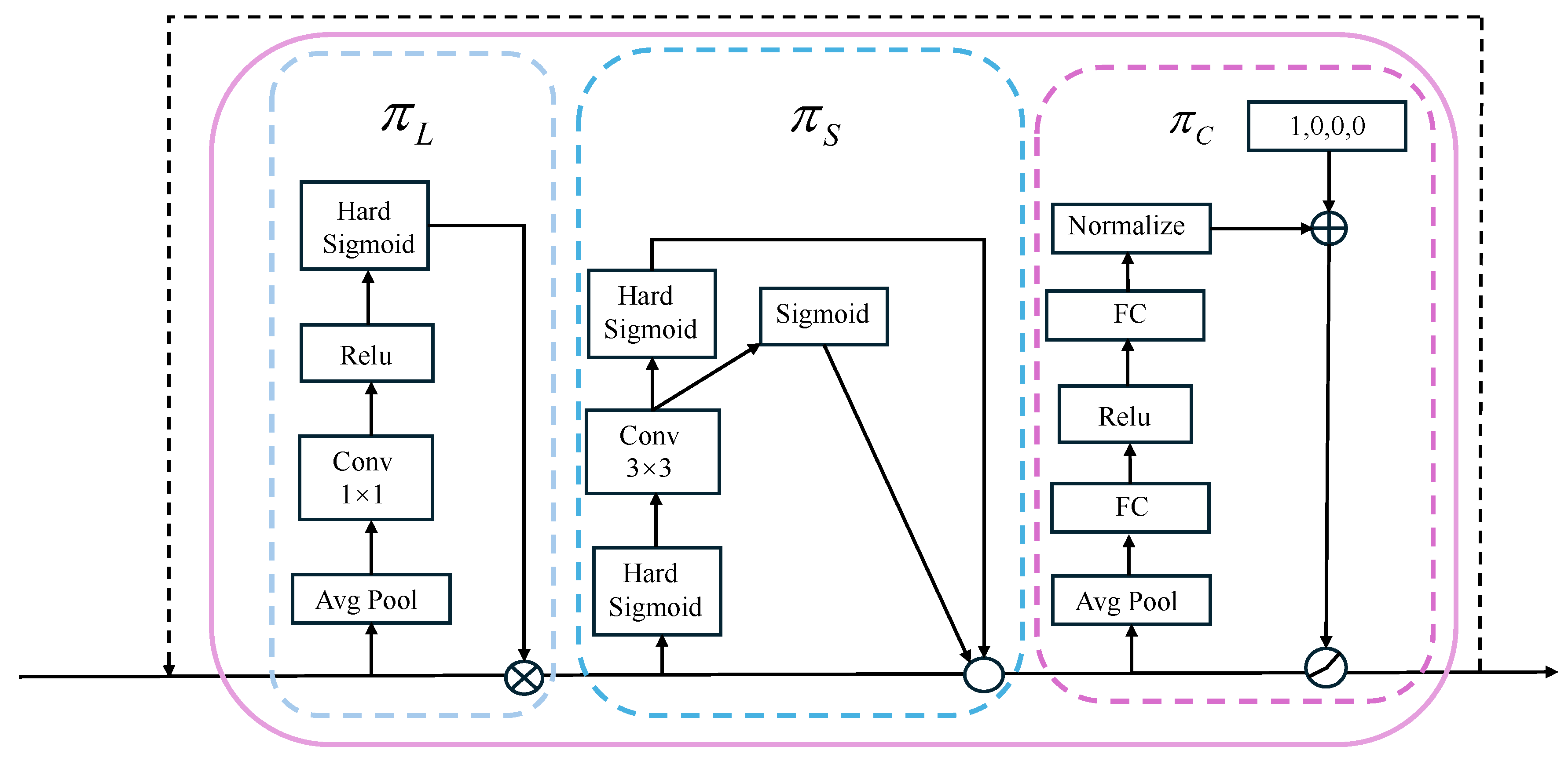
In dynamic landing tasks, when the flight altitude is high, the landing target is usually smaller, and the detection difficulty increases accordingly. In recent years, Dyhead, as a novel dynamic detection head framework, has significantly improved the performance of small target detection and object detection in complex scenes [40]. Dyhead improves the capability of the detection head by incorporating several self-attention layers, which allows for better feature representation and enhanced focus on important regions within the input data, combining the scale, space, and task perception mechanisms of different feature layers, spatial positions, and task-related channels to achieve more efficient feature representation. More importantly, this optimization does not increase significant computational overhead. Its architecture is shown in Figure 7:

In Figure 7, from left to right, the first is ${\pi }_L$, which is the scale-aware attention mechanism and can be expressed as follows:

$${\pi }_L\left(\mathcal{F}\right)\mathcal{F}=\sigma \left(f\left({\displaystyle \frac{1}{S}}{\displaystyle \frac{1}{C}}\sum _{s=1}^S\sum _{c=1}^C{\mathcal{F}}_{s,c}\right)\right)\mathcal{F}$$

(1)

In Equation (1), $\mathcal{F}\in {\mathbb{R}}^{L\times H\times W\times C}$ refers to a tensor with four dimensions representing the feature pyramid. The first dimension, L, corresponds to the total number of levels, while H and W capture the height and width of the spatial structure, respectively. Finally, C denotes the quantity of channels within each feature map. For computational efficiency, the tensor is reshaped into a three-dimensional structure $\mathcal{F}\in {\mathbb{R}}^{L\times S\times C}$, where S is the total spatial dimension of each layer, calculated as the product of height and width $S=H\times W$. The operation $f(·)$ performs a linear mapping, which is approximated using a $1\times 1$ convolution layer. Additionally, the hard sigmoid activation $\sigma \left(x\right)$ is defined as $max(0,min(1,x+{\displaystyle \frac{x+1}{2}}))$ and is applied to map the output values to the range [0, 1]. This simple yet efficient nonlinear activation function helps reduce the computational burden while improving performance by providing a smooth, bounded output.

The second one is ${\pi }_S$, which is the spatial perception attention, and its equation can be written as follows:

$${\pi }_S\left(\mathcal{F}\right)\mathcal{F}={\displaystyle \frac{1}{L}}\sum _{l=1}^L\left[\sum _{k=1}^K{w}_{l,k}\mathcal{F}(l,p_k+\Delta p_k,c)\Delta m_k\right]$$

(2)

Method ${\pi }_S$ involves two main steps: sparse attention learning and cross-layer feature aggregation at the same spatial position. First, the method performs sparse sampling at k positions, where each position is denoted as $p_k$. A self-learned spatial offset, $\Delta p_k$, shifts the sampling position from $p_k$ to $p_k+\Delta p_k$. This modification enables the model to concentrate more accurately on the discriminative regions within the feature map. Additionally, $\Delta m_k$ is a scalar representing the importance of the feature at the adjusted position $p_k+\Delta p_k$, and is learned through the training process. At the intermediate layer of $\mathcal{F}$, the feature activations are used to generate both $\Delta p_k$ and $\Delta m_k$.

By leveraging these learned spatial offsets and importance scalars, the method enables the model to selectively attend to the most relevant areas within the input feature maps. It can allocate varying significance to each spatial position, thereby improving the overall detection performance by focusing on critical areas of the feature map.

Finally, ${\pi }_C$ represents the attention mechanism tailored to the task at hand, and its equation can be expressed as follows:

$${\pi }_C\left(\mathcal{F}\right)\mathcal{F}=max\left[\left({\alpha }^1\left(\mathcal{F}\right){\mathcal{F}}_c+{\beta }^1\left(\mathcal{F}\right)\right),\left({\alpha }^2\left(\mathcal{F}\right){\mathcal{F}}_c+{\beta }^2\left(\mathcal{F}\right)\right)\right]$$

(3)

Equation (3) divides the feature map into two key terms to separately capture and adjust different contributions or interactions, $F_c$ represents the portion of the feature map linked to the c-th channel. The vector $[{\alpha }^1;{\beta }^1;{\alpha }^2;{\beta }^2]={\theta }^{*}(·)$ represents an extended function designed to learn and regulate the activation threshold. The function ${\theta }^{*}(·)$ is implemented in several stages. Initially, average pooling is applied across the $L\times S$ dimensions to reduce the feature’s size. The pooled features undergo two fully connected layers for learning intricate patterns, followed by normalization to standardize the outputs. Finally, the outputs are mapped to the interval $[-1,1]$ through the application of the sigmoid function, which enables the model to dynamically adjust the activation level of the features based on the learned threshold.

2.5. Optimization of Loss Function

In the YOLO task, an appropriate loss function is chosen to guide model convergence and ensure task completion. The Probabilistic IoU (ProbIoU) used in YOLOv8 OBB is an effective method for measuring the overlap between oriented bounding boxes (OBBs). Based on the Hellinger distance, ProbIoU assesses the similarity between two OBBs by calculating their covariance matrices and the differences in their center coordinates. Specifically, ProbIoU can be computed using the following equation:

$$\begin{array}{cc}\hfill D_B=& {\displaystyle \frac{1}{4}}{\displaystyle \frac{(a_1+a_2){(y_1-y_2)}^2+(b_1+b_2){(x_1-x_2)}^2}{(a_1+a_2)(b_1+b_2)-{(c_1+c_2)}^2}}\hfill \\ \hfill & +{\displaystyle \frac{1}{2}}{\displaystyle \frac{(c_1+c_2)(x_1-x_2)(y_1-y_2)}{(a_1+a_2)(b_1+b_2)-{(c_1+c_2)}^2}}\hfill \\ \hfill & +{\displaystyle \frac{1}{2}}ln\left({\displaystyle \frac{(a_1+a_2)(b_1+b_2)-{(c_1+c_2)}^2}{4\sqrt{(a_1{b}_1-c_1^2)(a_2{b}_2-c_2^2)}}}\right)\hfill \end{array}$$

(4)

In Equation (4), $D_B$ represents the Bhattacharyya distance, a metric that quantifies the geometric similarity between two oriented bounding boxes (OBBs). This distance is calculated by considering the covariance matrices of the two oriented bounding boxes (OBBs), represented by $a_1,b_1,c_1$ for the first OBB and $a_2,b_2,c_2$ for the second OBB. Additionally, the difference in their center coordinates, given by $(x_1-x_2)$ and $(y_1-y_2)$, is also factored in. The covariance matrices describe the orientation, shape, and spread of each OBB, while the differences in center coordinates capture their relative positions. The resulting value of $D_B$ provides a measure of how closely the two OBBs align geometrically. This distance is then used to compute the Probabilistic IoU (ProbIoU), which assesses the overlap between the OBBs. Ultimately, the final result of the ProbIoU is determined by the following:

$$\begin{array}{c}\hfill ProbIoU=1-\sqrt{1-e^{-D_B}}\end{array}$$

(5)

While ProbIoU is effective in assessing the overlap between bounding boxes, the introduction of Complete IoU (CIoU) significantly improves the accuracy of the evaluation. CIoU extends ProbIoU by adding an aspect ratio consistency term, which is expressed in the following equation:

$$\begin{array}{c}\hfill CIOU=ProbIoU-v\alpha \end{array}$$

(6)

Here, the aspect ratio consistency term v is defined as follows:

$$\begin{array}{c}\hfill v={\displaystyle \frac{4}{{\pi }^2}}{\left({tan}^{-1}\left({\displaystyle \frac{w_2}{h_2}}\right)-{tan}^{-1}\left({\displaystyle \frac{w_1}{h_1}}\right)\right)}^2\end{array}$$

(7)

The weight $\alpha$ is then used to adjust the influence of the aspect ratio on the final IoU value; this can be obtained from the following:

$$\begin{array}{c}\hfill \alpha ={\displaystyle \frac{v}{v-ProbIoU+(1+ϵ)}}\end{array}$$

(8)

This enhancement allows CIoU to capture the geometric relationships between OBBs more comprehensively, thereby improving the detection performance.

However, while CIoU enhances accuracy, it primarily focuses on the aspect ratio and does not fully capture the relationship between the bounding box’s width, height, and its confidence. To address this limitation, we replace CIoU with the EIoU loss function in ProbIoU. EIoU incorporates not just the center distance, but also the differences in area and size of the bounding box, enhancing both the stability and precision of target box regression.

The EIoU loss function is defined as follows:

$$\begin{array}{cc}\hfill L_{EIOU}=& L_{dis}+L_{IoU}+L_{asp}\hfill \\ \hfill =& 1-\mathrm{IoU}+\rho {(b,b_{gt})}^2{\displaystyle \frac{1}{C_d^2}}+\rho {(w,w_{gt})}^2{\displaystyle \frac{1}{C_w^2}}+\rho {(h,h_{gt})}^2{\displaystyle \frac{1}{C_h^2}}\hfill \end{array}$$

(9)

where $L_{EIOU}$ is the expression of the overall loss, which consists of three losses: $L_{dis}$, $L_{IoU}$, and $L_{asp}$. Specifically, $L_{dis}$ represents the loss function that quantifies the disparity in distance between the predicted center points and the corresponding ground truth center points of the bounding boxes. $L_{IoU}$ evaluates the degree of overlap between the predicted and actual bounding boxes by considering the ratio of their intersection to the total area covered by both. $L_{asp}$ penalizes discrepancies in shape between the estimated and true bounding boxes by ensuring their aspect ratios are closely aligned. The integration of these three components enables a more thorough refinement of the bounding box’s alignment, proportions, and dimensions, thereby enhancing the precision and robustness of the detection process.

2.6. Pixel Error Converted to Actual Distance Error

During the process of mobile target recognition and landing, the visual system detects the moving landing target as a pixel error, which must be converted into a distance error before it can be provided to the flight control system for flight control. This conversion involves using parameters such as camera focal length, pinhole imaging model, imaging relationship, and camera–target distance to convert the pixel error in the image coordinate system into the true distance error in the world coordinate system. The relevant camera parameters used in this article are shown in

Table 1. Camera specifications.

Camera Parameters	Value
Optical Aperture (f-stop)	f/2.25
Focal Length	3.35 mm
Diagonal Field of View	180°
Resolution	2592 × 1944 px

.

The error conversion process uses camera parameters, including the focal length $f_c$ and pixel size ($p_x,p_y$). For the Y-axis, the pixel error ${ϵ}_{\mathrm{camera}}$ is converted to the image width error $R_y$ in meters using the following:

$$R_y={ϵ}_{\mathrm{camera}}{\displaystyle \frac{M_y}{M_{y^{\prime }}}}{p}_y{10}^{-3}$$

(10)

Here, $M_y$ and $M_{y^{\prime }}$ are the pixel counts of the original and processed images, and $p_y$ is the physical pixel size.

To convert the image width error into the actual distance error in the geographic coordinate system, a proportional relationship between the original and processed images is used to scale the pixel size. Using the pinhole imaging model, we can obtain the following:

$${\displaystyle \frac{1}{h_c}}+{\displaystyle \frac{1}{v}}={\displaystyle \frac{1}{f_c}}$$

(11)

Here, $h_c$ (corrected distance) is obtained by subtracting the vehicle height from the radar-measured distance if the straight-line error exceeds 0.7 m. $f_c$ is the camera’s focal length, and v is the image height. Based on the principle of similar triangles, Equation (12) is established:

$${\displaystyle \frac{P_u}{R_y}}={\displaystyle \frac{h_c}{v}}$$

(12)

where $P_u$ is the distance between the quadcopter and the landing target, and its ratio to the image error $R_y$ equals the ratio of $h_c$ to v.

According to Equations (11)–(12), we can obtain the final true distance error in the world coordinate system $P_u$:

$$P_u={\displaystyle \frac{R_y{h}_c}{f_c}}-R_y$$

(13)

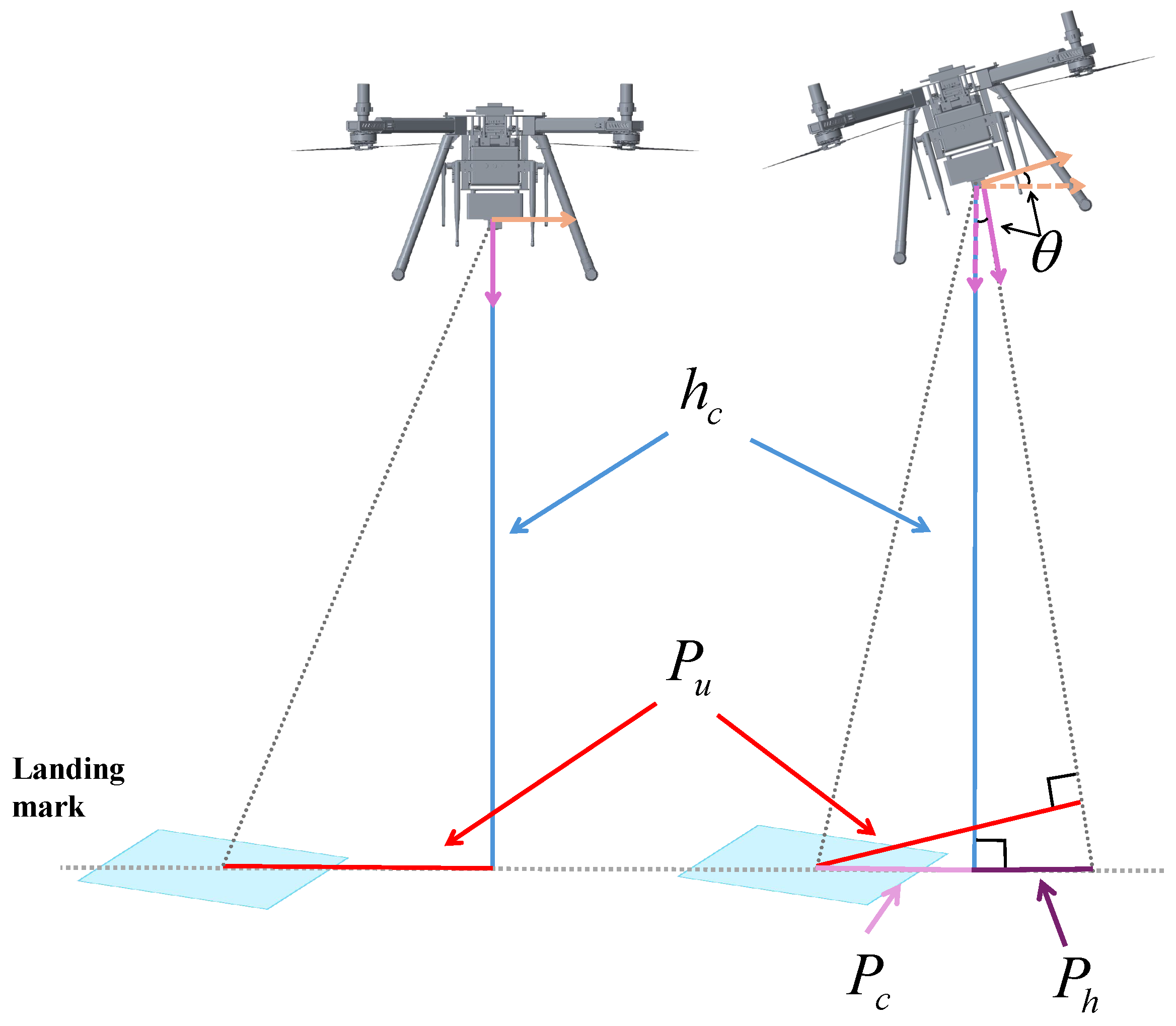
Since the camera used in this study is not equipped with a gimbal, the attitude angle generated during the quadcopter’s flight will impact the accuracy of the conversion in the above equation. Therefore, compensation is necessary to ensure that the pixel error can be accurately converted to the actual distance error, even when the quadcopter has an attitude angle. The conversion relationship is illustrated in Figure 8:

Figure 8. Compensation by attitude angle.

Figure 8. Compensation by attitude angle.

$$P_c={\displaystyle \frac{P_u}{cos\left(\theta \right)}}-P_h={\displaystyle \frac{P_u}{cos\left(\theta \right)}}-h_{c}tan\left(\theta \right)$$

(14)

Here, $P_c$ is the compensated distance error, $\theta$ is the quadcopter’s current attitude angle, and $P_h$ is the auxiliary calculated distance. Using Equations (10)–(14), the actual distance error available to the controller is successfully obtained using the detected pixel error.

3. Control System Design

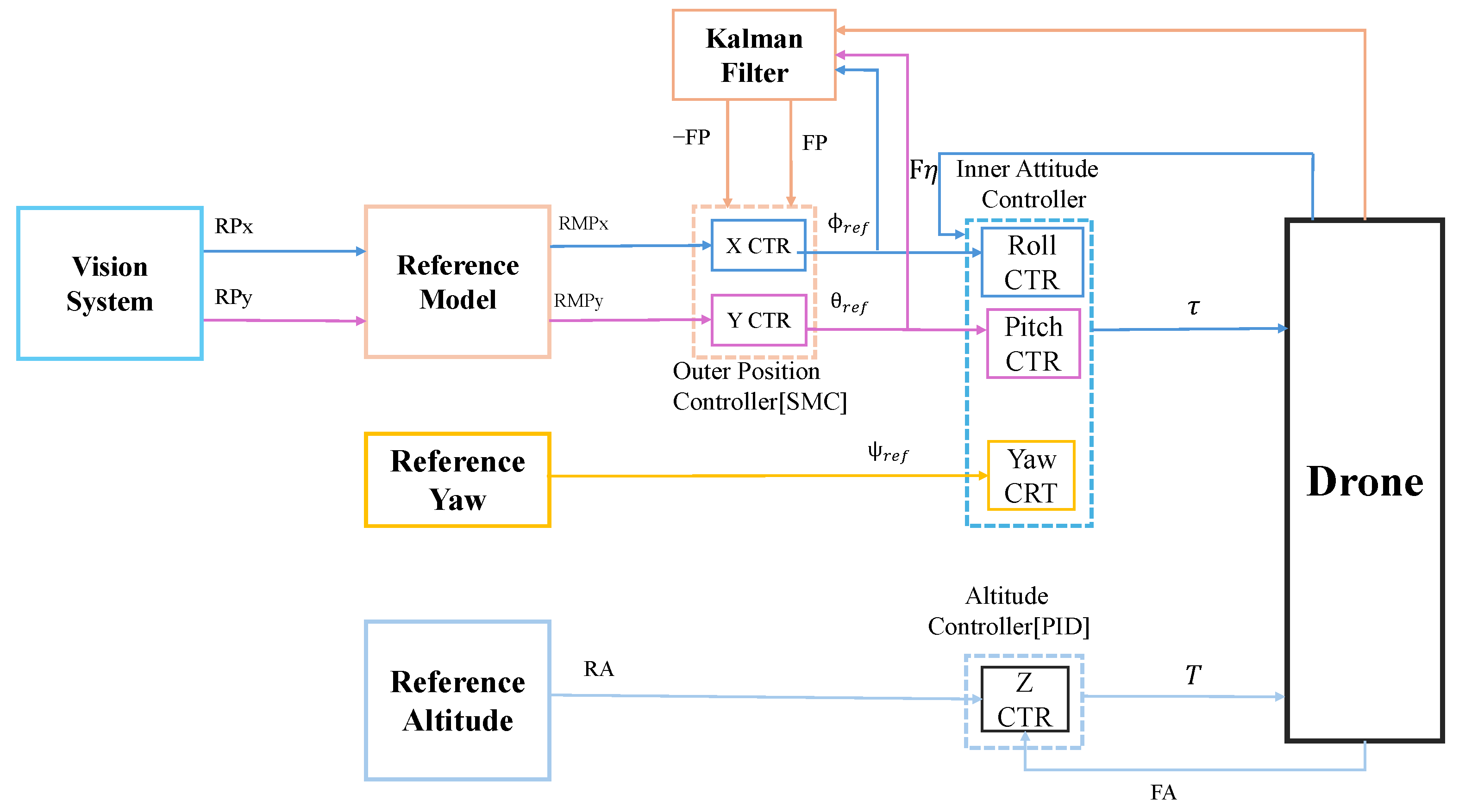
In a dynamic quadcopter visual landing system, identifying the landing target is crucial, but ensuring stable and reliable tracking during landing is equally important. To handle inevitable disturbances, the system incorporates sliding mode control, valued for its robustness against external interference. However, its application often generates large control outputs to counter deviations, potentially causing abrupt attitude changes during landing. To address this, a reference model is introduced to ensure smooth and safe state transitions, enhancing control safety without sacrificing performance. A Kalman filter is also employed to improve stability through accurate state estimation. Combining these, a sliding mode controller integrated with a reference model and Kalman filter is proposed, achieving safe and precise control during dynamic visual landing. The complete controller layout is shown in Figure 9.

Figure 9 depicts the control system architecture, which includes an outer loop for position control and an inner loop for attitude control. The outer loop generates the desired Roll and Pitch targets based on the quadcopter’s position, which are then fed into the inner control loop to compute required torque to achieve the desired attitude and motion, ensuring stable flight behavior. The establishment of the model can refer to our previous study [11].

3.1. Reference Model Design

The dynamics of the system are described by using the Newton–Euler formulation:

$$\left\{\begin{array}{c}\dot{\mathbf{r}}=\mathbf{v}\hfill \\ m\dot{\mathbf{v}}=-mg{\mathbf{e}}_z+\mathbf{R}{\mathbf{e}}_z\mathbf{F}\hfill \\ \dot{\mathsf{\varphi }}=\mathsf{\omega }\hfill \\ \mathbf{I}\dot{\omega }=-\omega \times \mathbf{I}\omega +\mathbf{M}\hfill \end{array}\right.$$

(15)

where $\mathbf{r}$ and $\mathbf{v}$ are the position and velocity, m is the mass, and g is the gravitational acceleration with unit vector ${\mathbf{e}}_z$. $\mathbf{F}$ is the total thrust, $\mathsf{\varphi }$ and $\mathsf{\omega }$ denote attitude and angular velocity, $\mathbf{I}$ is the inertia matrix, and $\mathbf{M}$ is the control torque.

Then, the three-axis virtual input quantities are introduced as defined in the following equations:

$$\begin{array}{cc}\hfill u_x& =\mathbf{F}\left(cos\varphi sin\theta cos\psi +sin\varphi sin\psi \right)\hfill \end{array}$$

(16)

$$\begin{array}{cc}\hfill u_y& =\mathbf{F}\left(cos\varphi sin\theta sin\psi -sin\varphi cos\psi \right)\hfill \end{array}$$

(17)

$$\begin{array}{cc}{u}_z\hfill & =\mathbf{F}cos\varphi cos\theta \hfill \end{array}$$

(18)

The position movement equations are simplified as in the following equations:

$$\begin{array}{cc}\hfill \ddot{x}& ={\displaystyle \frac{u_x}{m}}\hfill \end{array}$$

(19)

$$\begin{array}{cc}\hfill \ddot{y}& ={\displaystyle \frac{u_y}{m}}\hfill \end{array}$$

(20)

$$\begin{array}{cc}\hfill \ddot{z}& ={\displaystyle \frac{u_z}{m}}-g\hfill \end{array}$$

(21)

Finally, the general form of the position equations can then be rewritten as follows:

$$\dot{X}=AX+Bu$$

(22)

$$Y=CX$$

(23)

where the input matrix is defined as $B={[0,0,{\displaystyle \frac{1}{m}}]}^T$, the output matrix is $C=[1,0,0]$, and the A is given by the following:

$$A=\left[\begin{array}{ccc}0& 1& 0\\ 0& 0& 1\\ 0& 0& 0\end{array}\right]$$

In the entire control process, ensuring the safety and stability of the quadcopter is crucial. To achieve this, the quadcopter must be able to track the target in a stable manner, with minimal abrupt changes in the target value. Therefore, the design of the transition process for the tracking state plays a key role. In light of this, this paper proposes the design of a reference model to facilitate the smooth and comprehensive state transitions required during the control process.

The reference model is designed with the key consideration that $A_r$ must ensure the model’s stability and $(A_r,B_r)$ should be controllable.

$$\left\{\begin{array}{c}{\dot{X}}_{\mathrm{r}}=A_r{X}_r+B_{r}r\hfill \\ Y_r=C_r{X}_r\hfill \end{array}\right.$$

(24)

Here, $A_r$, $B_r$, $C_r$ are the reference state matrix, reference input matrix, and reference output matrix, respectively, and $X_r$ denotes the reference state associated with X, where the target values of position and velocity are expressed as ${[Po{s}_m,Ve{l}_m]}^T$. The structure of the matrix $A_r$ is as follows:

$$A_r=\left[\begin{array}{cc}0& 1\\ k_{m1}& k_{m2}\end{array}\right]$$

(25)

This matrix is crucial as it governs the change in the reference state. By designing the parameters $k_{m1}$ and $k_{m2}$, the tracking speed of the transition state can be adjusted. And $B_r=-B{\left(C_r{\left(A_r\right)}^{-1}B\right)}^{-1}$.

3.2. Design of Sliding Mode Controller

In order to enable the quadcopter to land stably and safely at the center of the moving target, we designed a sliding mode controller to help achieve this goal. Following the design of the Kalman filter and reference model, obtaining the reference transition state, and estimating the system states, the RMSMC can be designed. The difference between the quadcopter’s current state and the transition state given by the reference is defined as $E_x=X-X_r$, and the time derivative of the error, $\dot{E_x}$, can be computed as follows:

$$\begin{array}{c}\hfill \dot{E_x}=\dot{X}-\dot{X_r}\Rightarrow \\ \hfill \dot{E_x}=(A-A_r)X+A_r{E}_x+Bu-B_{r}r\end{array}$$

(26)

Then, the sliding surface can be designed as follows:

$$\sigma =S{E}_x$$

(27)

where $S\in {\mathbb{R}}^{3\times 1}$ is the weight vector that can be adjusted for each state error. Therefore, by differentiating Equation (27), we obtain the following:

$$\dot{\sigma }=S((A-A_r)X+A_r{E}_x+Bu-B_{r}r)$$

(28)

Once the sliding mode condition is met, the system reaches the sliding surface, meaning that, at this point, $\dot{\sigma }=\sigma =0$. Assuming $K_c=A-A_r$ and $K_0={\left(SB\right)}^{-1}S{B}_r$, the equivalent control input $u_{eq}$ is given by the following:

$$u_{eq}=-{\left(SB\right)}^{-1}S{K}_{c}X-{\left(SB\right)}^{-1}S{A}_r{E}_x+K_{0}r$$

(29)

In addition, to minimize the chattering caused by the sliding mode, a smooth function is used in this paper to replace the traditional sign function:

$$f\left(\sigma \right)={\displaystyle \frac{\sigma }{\left|\sigma \right|+\partial }}$$

(30)

Among them, ∂ is a parameter that can be adjusted artificially, which is related to the disturbance size. Therefore, the nonlinear output is defined as $U_{sw}=K_{sw}f\left(\sigma \right)$ where $K_{sw}=-m{\left(SB\right)}^{-1},m>0$ is the nonlinear gain. The final controller output is shown in the following equation:

$$u=u_{eq}+u_{sw}$$

(31)

To confirm the stability of the designed RMSMC, the Lyapunov function can be defined as follows:

$$V={\displaystyle \frac{1}{2}}{\sigma }^2$$

(32)

To find the time derivative of V, we proceed as follows:

$$\dot{V}=\sigma \dot{\sigma }$$

(33)

By incorporating the derivative of the sliding mode surface, we obtain the following equation:

$$\dot{V}=\sigma \left[S(K_{c}X+A_r{E}_x+Bu-B_{r}r)\right]$$

(34)

Simplify the expression by expanding and rearranging terms:

$$\begin{array}{cc}\hfill \dot{V}=\sigma [& S{K}_{c}X+S{A}_r{E}_x-S{K}_{c}X\hfill \\ \hfill & +S{B}_{r}r-S{A}_r{E}_x\hfill \\ \hfill & +SB{K}_{sw}f\left(\sigma \right)-S{B}_{r}r]\hfill \end{array}$$

(35)

Simplify further to the following:

$$\dot{V}=\sigma \left[SB{K}_{sw}f\left(\sigma \right)\right]$$

(36)

Substitute $K_{sw}=-m{\left(SB\right)}^{-1}$; we can obtain:

$$\dot{V}=\sigma \left[SB(-m{\left(SB\right)}^{-1})f\left(\sigma \right)\right]$$

(37)

Simplify further to the following:

$$\dot{V}=-m\sigma f\left(\sigma \right)\Rightarrow \dot{V}=-m{\displaystyle \frac{{\sigma }^2}{\left|\sigma \right|+\partial }}$$

(38)

Since both m and ∂ are set to positive values and can be adjusted, it follows that $\dot{V}\le 0$. Therefore, by the LaSalle invariance principle, the sliding mode controller designed above is asymptotically stable.

4. Simulation and Experiment

This section first presents the evaluation of the improved YOLOv8 OBB model, followed by experimental verification of the pixel error conversion. Finally, it provides validation of the controller and verification through actual flight tests.

4.1. Indicators of the Evaluation

This paper evaluates the improved model using precision, recall, mAP@0.5, and mAP@0.5:0.95. Precision measures the proportion of correctly identified positive samples, while recall indicates the model’s ability to detect all actual positives. The formulas for both metrics are as follows:

$$Precision={\displaystyle \frac{\mathrm{TP}}{\mathrm{TP}+\mathrm{FP}}}$$

(39)

$$Recall={\displaystyle \frac{\mathrm{TP}}{\mathrm{TP}+\mathrm{FN}}}$$

(40)

AP is the area under the precision–recall curve, and mAP is the average across categories. mAP@0.5 corresponds to an IoU threshold of 0.5, while mAP@0.5:0.95 averages over multiple IoU thresholds ($0.5\le IOU\le 0.95$). These metrics, along with C and K, provide a full evaluation of the YOLO model. Precision and recall at IoU threshold K are $P\left(K\right)$ and $R\left(K\right)$, as shown as follows:

$$\Delta R\left(k\right)=R\left(k\right)-R(k-1)$$

(41)

$$AP=\sum _{k=1}^{N}P\left(k\right)·\Delta R\left(k\right)$$

(42)

$$mAP={\displaystyle \frac{1}{C}}\sum _{k=1}^{N}P\left(k\right)·\Delta R\left(k\right)$$

(43)

4.2. Experimental Dataset

During the data collection process, the first-level landing target in this paper is a self-designed pattern of 50 cm × 50 cm attached to a 1 m × 1 m wooden board, and the other secondary guided landing target is a vehicle. During the data collection process, photos of the first-level, secondary, and mixed landing targets at different heights and angles were taken at different time periods such as daytime (strong sunlight, weak sunlight) and night. At the same time, photos of the wrong landing points without targets and wrong patterns were taken. The quadcopter took images of 1920 × 1080 pixels at high altitude. The collected images were flipped, denoised, and color converted to enhance the richness and robustness of the dataset. After collecting the data, the roLabelImg open source software (https://github.com/cgvict/roLabelImg (accessed on 29 Jun 2020); version 1.8.6.) was used to mark the targets in the image to complete the annotation of the datasets.

4.3. Process of Model Training

The model was trained in a Windows 11 environment, utilizing a GeForce RTX3090Ti GPU and an Intel(R) Core(TM) i7-14700K CPU. Python 3.8.18 was used for application development; the deep learning framework was Pytorch 2.2.1, CUDA 11.8. The model was trained with the following initial settings: an input image size of 640 × 480, a warmup period of 5 epochs, a weight decay of 0.0003, and a total of 200 training epochs.

4.4. Ablation Experiments

4.4.1. Attentional Mechanisms’ Experiment

In this experiment, we incorporated different attention mechanisms with different coordinate configurations after the initial convolutional layer and trained the model on the public VisDrone/DroneVehicle dataset. The results are summarized in the

Table 2. Performance comparison of YOLOv8 OBB and its variants with different attention modules.

Methods	Parameters (M)	Gflops	mAP0.5 (%)	mAP0.5:0.95 (%)	Precision (%)	Recall
Baseline (YOLOv8_obb)	3.083	8.44	74.3	50.51	74.93	0.70401
Baseline + CA	3.09	8.453	74.768	50.865	73.946	0.705
Baseline + ShuffleAttention	3.083	8.446	74.872	51.109	76.004	0.699
Baseline + GAM	3.518	8.794	75.7	51.427	76.338	0.712
Baseline + CBAM	3.092	8.46	75.4	51.392	76.818	0.705

. As observed, under various attention mechanisms, the $\mathrm{mAP}@0.5$:$0.95$ is 0.882 percentage points higher than the baseline network and 0.572 percentage points higher than CA. Although it is 0.035 percentage points lower than GAM, the parameter count is significantly lower than that of GAM. Therefore, CBAM demonstrates the most noticeable improvement overall.

4.4.2. Loss Function

This section presents an evaluation of the performance of several loss functions, including CIoU, DIoU, and EIoU, on the public VisDrone/DroneVehicle dataset.

Table 3. Performance comparison of YOLOv8 OBB and its variants with different loss functions.

Methods	mAP0.5 (%)	mAP0.5:0.95 (%)	box_loss	dfl_loss	cls_loss
Baseline (YOLOv8_obb)	74.295	50.509	0.742	1.543	0.516
Baseline + CIoU	75.702	51.403	0.718	1.377	0.519
Baseline + DIoU	75.419	51.556	0.756	1.577	0.492
Baseline + EIoU	75.843	51.592	0.718	1.374	0.498

displays the experimental results. As observed, the EIoU loss function outperforms the others, with a 0.198% improvement over the CIoU loss function and a 0.036% improvement over the DIoU loss function based on the mAP@0.5:0.95.

4.4.3. Detect Head

This section assesses the effectiveness of various detection heads, including LSCD, LSDECD, LADH, and Dyhead, on the public VisDrone/DroneVehicle dataset.

Table 4. Performance comparison of YOLOv8 OBB and its variants with different detection heads.

Methods	Parameters (M)	Gflops	mAP0.5 (%)	mAP0.5:0.95 (%)	Precision (%)	Recall
Baseline (YOLOv8_obb)	3.083	8.441	74.301	50.511	74.931	0.704
Baseline + LSCD	2.381	6.727	72.542	50.421	70.954	0.689
Baseline + LSDECD	2.597	5.406	74.761	53.308	73.949	0.726
Baseline + LADH	3.128	8.081	69.451	48.337	71.857	0.699
Baseline + Dyhead	3.323	7.716	77.315	53.078	76.596	0.728

presents the experimental results. As observed, under different detection head mechanisms, the mAP@0.5:0.95 is 2.586% higher than the baseline network, 2.685% higher than LSCD, 4.741% higher than LADH, and 0.23 percentage points lower than LSDECD. However, the mAP@0.5 is 2.554% higher than LSDECD. Overall, Dyhead performs the best.

4.4.4. Model Improvement Results

Finally, we conducted ablation experiments on both public and private datasets. The first row represents the baseline YOLOv8 OBB model, and the second to fourth rows correspond to the progressively improved models, where “” indicates the activation of the introduced modules.

As shown in

Table 5. Comparison of different configurations in VisDrone/DroneVehicle.

YOLOv8_obb	CBAM	Dyhead	EIoU	Parameters (M)	Gflops	mAP0.5 (%)	mAP0.5:0.95 (%)
✓				3.083	8.441	74.291	50.501
✓	✓			3.092	8.462	75.401 (+1.11)	51.391 (+0.89)
✓	✓	✓		3.332	7.711	76.891 (+2.6)	52.712 (+2.211)
✓	✓	✓	✓	3.332	7.721	77.394 (+3.103)	53.114 (+2.613)

, on the public dataset, the improved model demonstrates a 3.1% increase in the mAP@0.5:0.95 and a 2.61% improvement in the mAP@0.5, compared to the baseline.

As shown in

Table 6. Comparison of different configurations in MarkWithCar.

YOLOv8_obb	CBAM	Dyhead	EIoU	Parameters (M)	Gflops	mAP0.5 (%)	mAP0.5:0.95 (%)
✓				3.082	8.441	95.900	69.301
✓	✓			3.091	8.452	96.301 (+0.401)	69.902 (+0.601)
✓	✓	✓		3.331	7.722	96.303 (+0.403)	71.102 (+1.801)
✓	✓	✓	✓	3.331	7.722	96.403 (+0.503)	71.403 (+2.102)

, on the private dataset, the improved model achieves a 0.5% higher mAP@0.5:0.95 and a 2.1% higher mAP@0.5 compared to the baseline model.

In conclusion, we evaluated the model on both the VisDrone/DroneVehicle and private datasets. This is shown in Figure 10, where Figure 10a,c represent the performance results of YOLOv8 OBB, and Figure 10b,d represent the performance results of our improved model. As observed in the figure, the improved model enhances vehicle recognition accuracy by 0.07 on the VisDrone/DroneVehicle dataset. On the private dataset, both vehicle and mark recognition accuracies are improved by 0.05. In summary, our improved model effectively enhances both recognition accuracy and precision.

To assess the robustness of the model, we conducted tests in various environmental conditions, as shown in Figure 11. These tests included scenarios with rain, strong sunlight reflection (which caused the small mark to appear white), and night-time street lighting. The results demonstrate that our model can accurately detect landing targets, exhibiting a degree of safety and stability across these challenging environments.

4.5. System Verification

Experiment Platform

This paper employs a quadcopter, the structure and key sensors of which are depicted in Figure 12. The flight control system and several sensors of the quad-rotor were developed within our laboratory. The quadcopter is equipped with a six-axis inertial measurement unit (IMU), a geomagnetic sensor (MAG), a GNSS, a flight data recorder (FDR), LEDs, an NVIDIA AGX, a radar, and various other modules. With an arm length of 0.762 m and a total weight of 5.7 kg, the quad-rotor is engineered for superior performance and versatility.

4.6. The Verification of Pixel Conversion Result

To assess the efficacy of the proposed pixel conversion method and attitude angle range error compensation, two experiments were conducted. The first experiment focused on validating the pixel conversion process. As shown in Figure 13, a landing identification target was placed beneath the camera while the quadcopter maintained a fixed altitude. The landing mark was shifted along the aircraft’s X-axis in 20 cm steps. The flight control system recorded the range error data to evaluate the precision of the proposed pixel conversion method.

Figure 14 displays the data of the conversion verification experiment. In Figure 14a,b, the solid red line represents the actual distance measured in meters; meanwhile, the blue dotted line represents the distance calculated after the conversion. According to the gap in data, it can be seen that the distance conversion performed by the visual system is both accurate and reliable.

It can also be found from

Table 7. Analysis of fixed-angle pixel error conversion.

Parameter	True Value	Distance Max Error
X Distance (m)	[−0.4, 0.4]	0.017
Y Distance (m)	0.0	0.0039

, that the gap between our converted distance error and the given standard value is very small, proving that our proposed conversion method is effective and feasible.

The second experiment tests attitude angle compensation by tilting the quadcopter, holding it, and repeating the process while calculating distance error, without using a gimbal.

As the quadcopter tilts, compensations are applied to the front and rear X-axis (Pitch), Y-axis (Roll), and height based on the attitude angle information. Figure 15 shows the results of the height and position error compensation. Both distance and height are measured in meters. In Figure 15a, the quadcopter’s attitude angle is shown in degrees. Figure 15b shows height compensation, with actual, pre-compensation, and post-compensation heights represented by red, solid blue, and light blue dotted lines, respectively. Figure 15c and Figure 15d show the attitude angle compensation for X and Y axis distance errors, with similar line conventions. These results confirm the method’s effectiveness.

Table 8. Comparison of height and distance before and after compensation.

Parameter	Without Compensation	With Compensation (Increase)	True Value
Measuring Height (m)	2.54 to 2.72	2.50 to 2.57 ($\mathbf{95}\%\uparrow$)	2.54
Measuring X Distance (m)	−0.84 to −0.77	−0.82 to −0.78 ($\mathbf{74}.\mathbf{32}\%\uparrow$)	−0.8
Measuring Y Distance (m)	0.93 to 1.27	1.18 to 1.28 ($\mathbf{96}.\mathbf{2}\%\uparrow$)	1.22

describes the height and distance errors before and after compensation. Table 8 shows that the maximum error of height before compensation reaches 0.18 m, while after compensation it is only 0.028 m, and the error is reduced by 84%. When the Roll angle moves, the distance measurement in the Y direction is significantly influenced by the attitude change, and the maximum error of the Y direction before compensation reaches 0.2922 m, while after compensation it is only 0.049 m, and the error is reduced by 83.6%.

4.7. Dynamic Landing Tracking Experiment

The specific design process of the sliding mode controller follows the procedure outlined in [11]. The dynamic platform moves at an average speed of about 1 m/s and the actual flight experiment environment is shown in Figure 16:

During the flight, the drone visual recognition map is as shown in Figure 17:

This experiment demonstrated the quadcopter’s control performance using a sliding mode controller integrated with the YOLOv8 visual tracking system, as illustrated in Figure 18. For position tracking, Figure 18a shows the reference position in red, while the actual tracking position is depicted by the blue dashed line. The results show that the sliding mode controller accurately tracks the reference trajectory, with the largest tracking error observed being 0.356 meters. The speed tracking performance is shown in Figure 18b, where the red line is the reference speed; meanwhile, the blue dashed line shows the actual speed, with the maximum recorded tracking error being 0.1258 m/s. Errors in position and speed tracking are detailed in Figure 19. In terms of visual tracking, Figure 18c,d display the tracking deviations in the north and east components. The northward tracking error gradually converges to within 0.13 m after the initial phase, reducing to 0.08 m upon landing. Meanwhile, the eastward tracking error remains stable within 0.25 m, with a final landing error of 0.11 m. The maximum error magnification before landing is shown in Figure 20. Throughout the process, the landing target was consistently detected.

This experiment verifies the effectiveness of the sliding mode controller and YOLOv8 visual tracking system in the dynamic landing of the UAV. As summarized in

Table 9. Summary of quadcopter landing experiment results.

Parameters	Metric	Maximum Error	Final Error
Position Tracking	Reference vs. Actual Position	0.36 m	−
Speed Tracking	Reference vs. Actual Speed	0.13 m/s	−
Visual Tracking (N)	Northward Deviation	0.13 m	0.08 m
Visual Tracking (E)	Eastward Deviation	0.25 m	0.11 m

, the maximum position tracking error is 0.356 m, and the maximum velocity tracking error is 0.1258 m/s, showing good trajectory tracking ability. In terms of visual tracking, the north and east position deviations converge to 0.08 m and 0.11 m, respectively, showing the tracking ability of the system in dynamic landing. The overall experimental results prove the stability and robustness of the method in dealing with complex scenes, and provide reliable support for the dynamic landing of the UAV. Overall, the sliding mode controller and the YOLOv8 visual system show good robustness, providing reliable support for the dynamic landing of the UAV, thus proving the effectiveness and reliability of the method in actual scenes.

5. Discussion

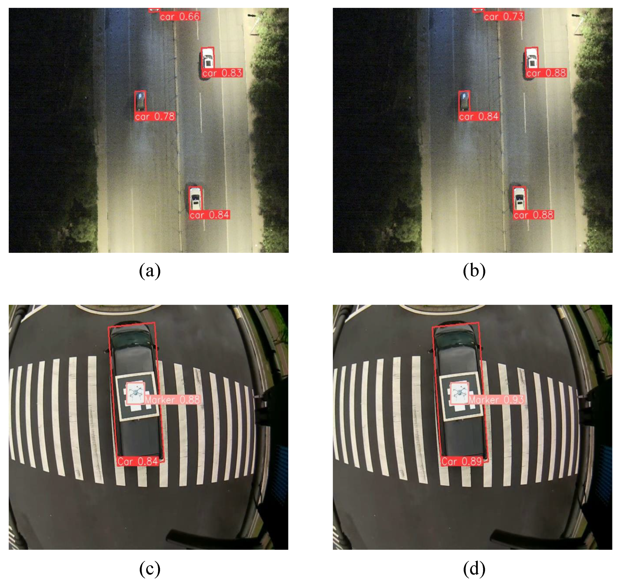
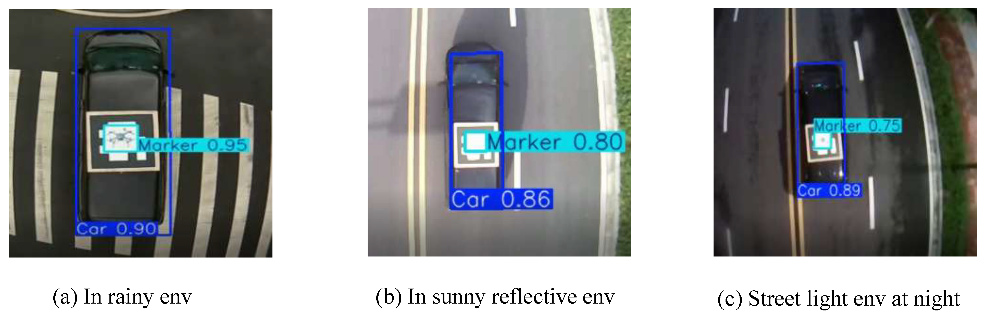
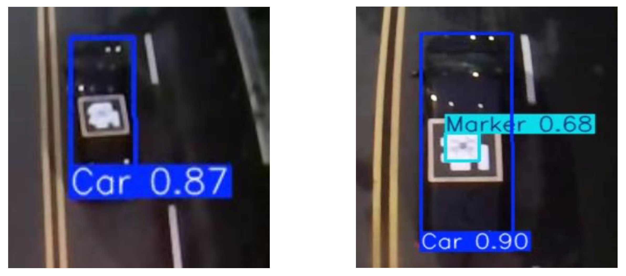
The improved dynamic landing system proposed in this paper has demonstrated effectiveness in key aspects such as target detection, pixel conversion, and dynamic landing control. Comprehensive experimental results show that, for the baseline YOLOv8 OBB model, challenges commonly encountered during the landing process—such as difficulties in identifying small targets and the presence of complex, high-background environments—were addressed by integrating the CBAM attention mechanism, the DyHead detection head, and the EIoU loss function. These enhancements led to a steady improvement in recognition accuracy across both public and private datasets, validating the effectiveness of each module in boosting model performance and target detection accuracy within the experimental setting.

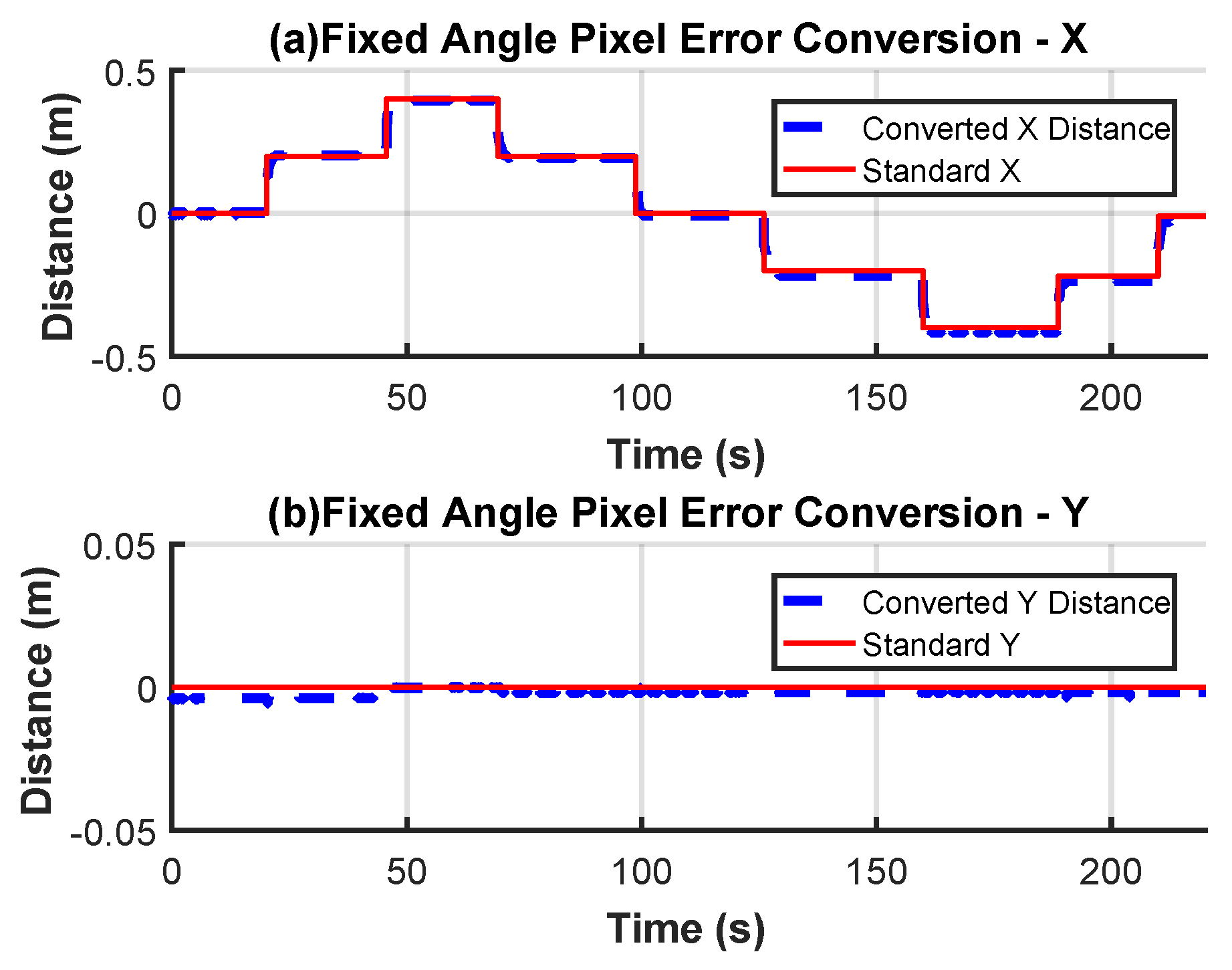
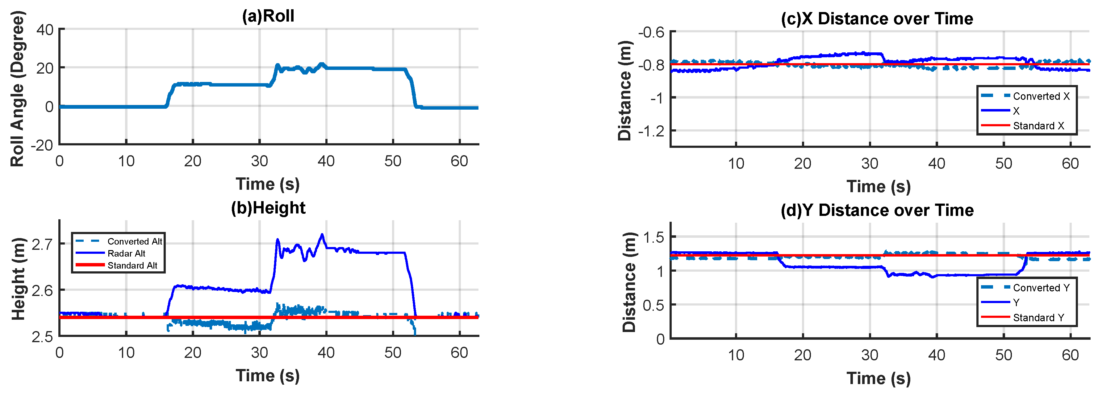
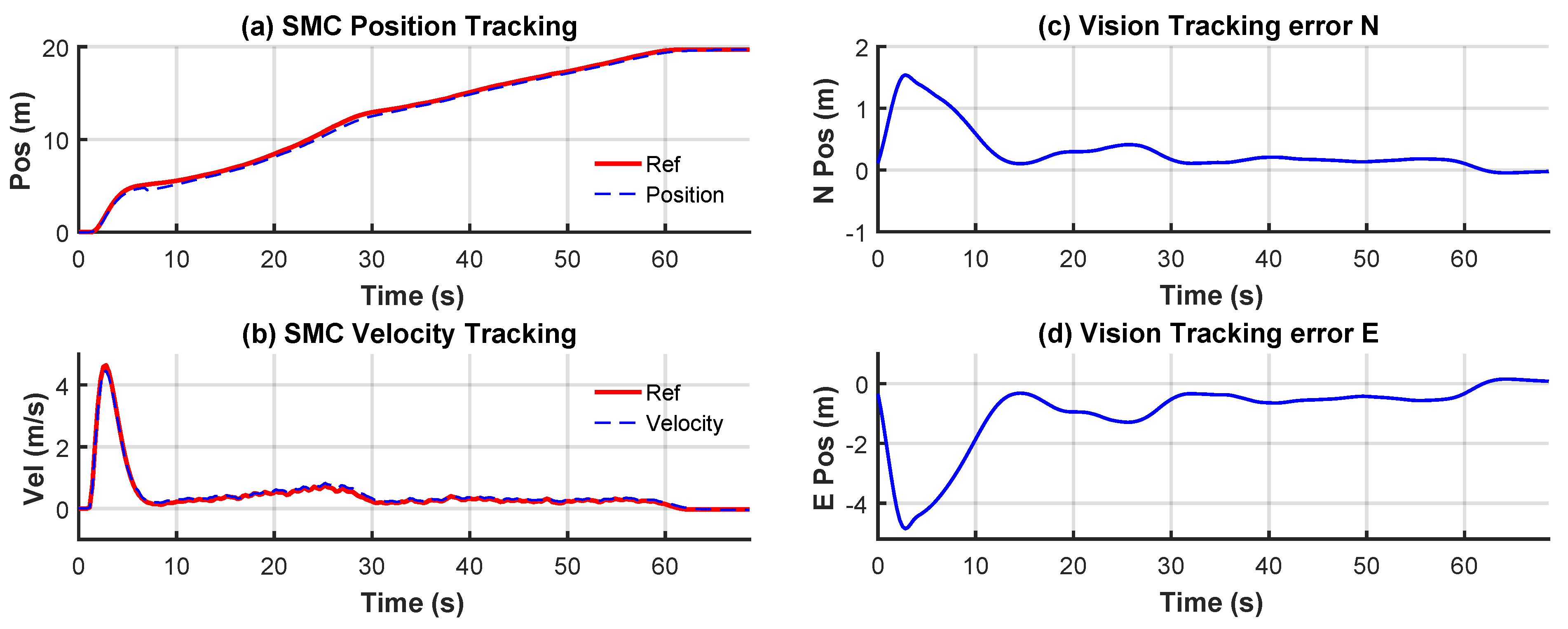
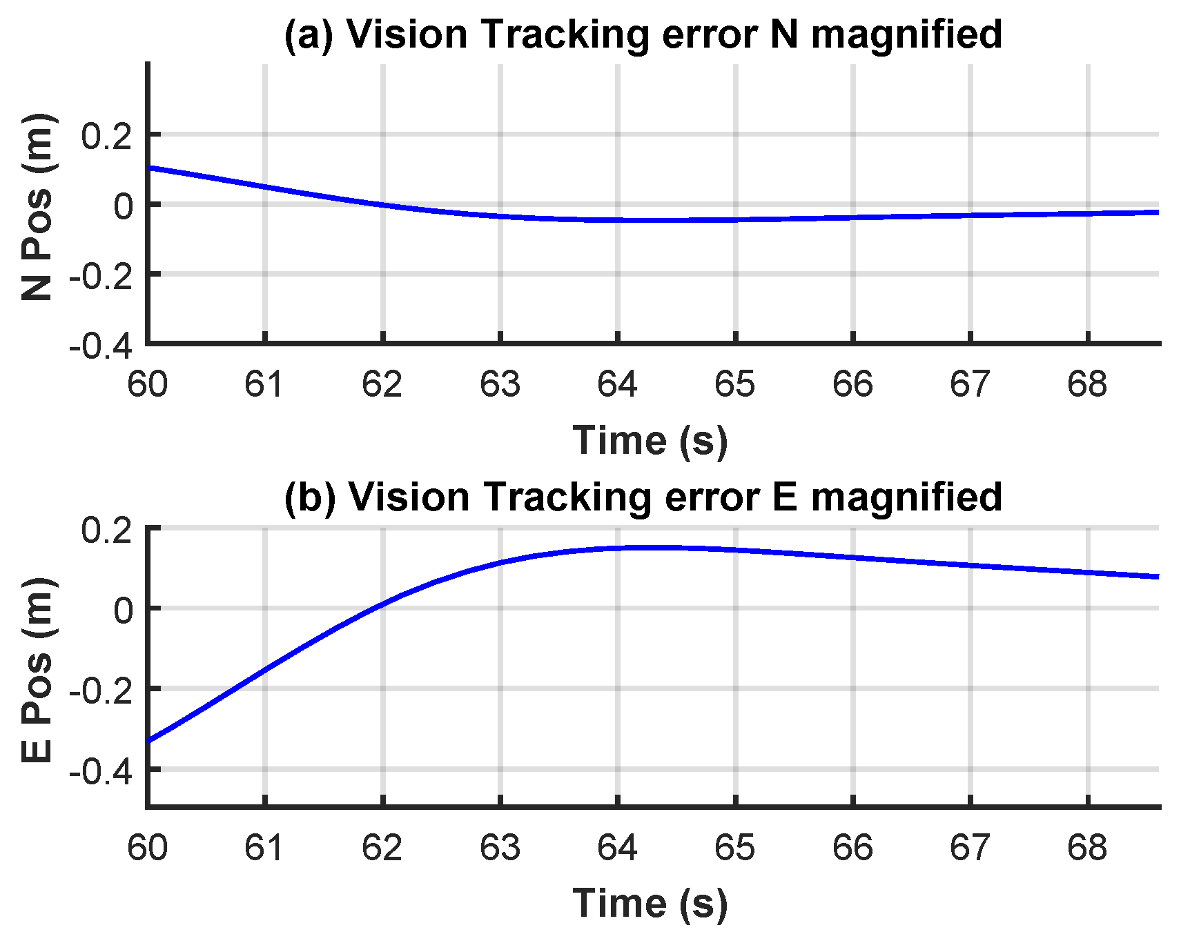
Additionally, for landing guidance in the control process, experiments on pixel error conversion and attitude angle compensation revealed that the proposed conversion algorithm and compensation strategy not only significantly reduced measurement errors under fixed height and varying attitudes but also provided precise position information for subsequent dynamic control. Furthermore, dynamic landing experiments employing a sliding mode controller demonstrated that the system maintained low maximum position and velocity errors while tracking the reference position, ensuring the successful completion of the landing task.

In conclusion, this study enhanced the accuracy and stability of UAV target detection and visual tracking by optimizing the landing recognition algorithm and implementing a sliding mode controller based on a reference model. However, future work should further explore the adaptability and robustness of the proposed approach in larger-scale environments with dynamic and unpredictable conditions.

6. Conclusions

This paper designs and implements a dynamic quadcopter landing system with drone vision and sliding mode control. Landing target detection uses the improved YOLOv8 OBB algorithm. CA, Dyhead, and EIoU Loss are added to the original model to improve the accuracy of the detection. Then, the detected pixel error is converted to the actual position error. At the same time, the attitude compensation is corrected. Furthermore, in order to ensure the stability and rapidity of tracking, a position sliding mode controller based on the reference model is designed, verified, and applied to help the quadcopter track the landing target. Finally, the practicality of the proposed system is ultimately validated through real-world flight experiments. The results demonstrate that the improved YOLOv8 OBB demonstrates an improvement in the mAP0.5:0.95 index by 2.23 percentage points. The position tracking error is always below 0.2 m, and the final landing error is 0.11 m, which proves that the system in this paper can complete accurate dynamic landing.

However, it should be noted that, although the RMSMC has a resistance to disturbances, no additional artificially generated interference was added in this experiment. In future research, we will add additional interference factors, such as continuous wind interference or a swaying landing surface.