Article

Modeling Non-Equilibrium Rarefied Gas Flows Past a Cross-Domain Reentry Unmanned Flight Vehicle Using a Hybrid Macro-/Mesoscopic Scheme

1
Hypersonic Technology Laboratory, National University of Defense Technology, Changsha 410073, China
2
College of Aerospace Science and Engineering, National University of Defense Technology, Changsha 410073, China
*
Author to whom correspondence should be addressed.
Drones 2025, 9(4), 239; https://doi.org/10.3390/drones9040239
Submission received: 17 February 2025 / Revised: 13 March 2025 / Accepted: 21 March 2025 / Published: 24 March 2025

Abstract

The cross-domain reentry unmanned flight vehicle passes through thin atmospheres and dense atmospheres when it comes across atmospheres in the near-space area. For the early transition regime, the classical macroscopic and mesoscopic approaches are either not accurate or computational too expensive. The hybrid macro-/mesoscopic method is proposed for simulating rarefied gas flows past a cross-domain reentry spheroid–cone unmanned flight vehicle in the present study. The R26 moment scheme is applied in the main flow from a macroscopic point of view, and the discrete velocity method (DVM) is used for solving the Boltzmann equation from a mesoscopic point of view. The simulation results show that the hybrid macro-/mesoscopic scheme is well-suited for non-equilibrium rarefied gas flows past a cross-domain reentry unmanned flight vehicle. The results obtained in this study are consistent with benchmark results, with a maximum density error of 9%. The maximum errors of the heat transfer coefficient and pressure coefficient are 2% and 4.6%, respectively. In addition, as the Knudsen number (Kn) becomes larger, the thickness of the shock layer at the head of the flight vehicle becomes thicker, and non-equilibrium effects become more critical for the aircraft. Since the Boltzmann–Shakhov equation has only been solved close to the wall of the spacecraft, the computational cost can be considerably saved.

1. Introduction

The near-space area bridges the atmospheric gap between the thin atmosphere and the dense atmosphere. Due to its unique airspace-location advantages, the adjacent space plays a crucial role in the struggle for air supremacy in modern warfare, high-precision rapid strikes, civilian communications, etc. The cross-domain reentry unmanned flight vehicle passes through free molecular, transition, slip, and continuum regimes when it comes across the atmosphere in the near-space area [1,2]. Due to the rarefied effect, the thermodynamics and the aerothermodynamics around space vehicles are totally different in various flow regimes [3], include high temperature, high pressure, high speed, etc. The traditional Navier–Stokes–Fourier (NSF) equation and the Fourier law based on the continuous flow assumption are not valid anymore. Additionally, solving the Boltzmann equation at the mesoscopic level is computational expensive and time-consuming [4]. Therefore, it is of great theoretical significance and engineering application prospect to develop a highly efficient and accurate numerical scheme to simulate the flow field and complex flow mechanism of aircraft in the whole flow domain.
Numerically, the flow field of the non-equilibrium rarefied gas flows past a cross-domain reentry unmanned flight vehicle can be described based on the mesoscopic or macroscopic method [4,5]. For the former, the direct simulation Monte Carlo (DSMC) method [6] and the discrete velocity method (DVM) [7] are the most popular schemes to solve the Boltzmann equation accurately. Specifically, the hypersonic non-equilibrium rarefied gas flows past the three-dimensional spacecraft have been widely simulated numerically [8,9]. For instance, the RAM-C II unmanned flight vehicle, Stardust reentry flight vehicle [8], and the Chinese lunar reentry capsule have been analyzed and evaluated against the benchmark data across various Knudsen and Mach numbers, and the DSMC method is able to present highly accurate results [9]. However, the DSMC scheme would suffer statistical noise for the low Mach or Knudsen numbers. For the deterministic approach, extensive works have been studied for simulating the rarefied gas flows based on nonlinear model Boltzmann equations, i.e., the Bhatnagar–Gross–Krook (BGK) model [10], the Shakhov model [11], the Ellipsoidal Statistical BGK model [12], and the Morse model [13]. The 1D shock-tube problems, rarefied gas flows past a 2D airfoil, and hypersonic flows past a 3D sphere–cone flight vehicle with different Kn, Re, and Ma numbers are simulated based on the high-order gas–kinetic unified algorithms (GKUA) [14]. Simulation results have indicated that the GKUA is able to provide accurate results for the reentry spacecraft application with a wide range of Kn numbers [14,15,16]. The Boltzmann equation’s complexity, particularly due to its multi-dimensional VDF and the intricate nonlinear collision term, makes its application to many real-world problems challenging. As a result, significant efforts have been made to develop alternative macroscopic modeling approaches to non-equilibrium flows.
The Navier–Stokes–Fourier (NSF) equations serve as the classical macroscopic framework for modeling gas flows. When supplemented with suitable velocity-slip and temperature-jump boundary conditions, they can capture key flow characteristics in weakly rarefied scenarios close to equilibrium, such as those in the slip regime. However, additional caution is required when thermal effects become significant [17]. To expand the use of macroscopic models into the transition regime, the G13 moment method was developed by Grad [18]. Using an approach similar to the Chapman–Enskog expansion, Struchtrup [19] regularized the G13 equations and obtained the R13 moment method. Gu and Emerson [20] and Struchtrup [21] derived the wall boundary conditions (WBCs) for the regularized 13 moment equations (R13) based on Maxwell’s kinetic WBC [22]. The R13 equations can accurately describe non-equilibrium effects for Knudsen numbers up to 0.25. Furthermore, Gu [23] expanded the moment scheme to develop the regularized 26 (R26) moment systems, which highlighted their capability as an effective engineering tool for analyzing non-equilibrium flows in the transition regime [24,25]. The moment method effectively connects traditional hydrodynamic models with kinetic models in the early transition regime, addressing the limitations of the NSF equations and the discrete velocity method (DVM), which are either insufficiently accurate or computationally inefficient. In this study, we integrated the R26 moment systems with the kinetic solver to model non-equilibrium rarefied gas flows around a cross-domain reentry unmanned flight vehicle.
The structure of the rest of this paper is outlined as follows. Section 2 provides a concise overview of the R26 moment scheme at the macroscopic level. The kinetic theory and the corresponding WBCs are described in Section 3. The hybrid macro-/mesoscopic scheme is also described in this section. Using the hybrid approach, Section 4 presents comprehensive results for simulating non-equilibrium rarefied gas flows around a cross-domain reentry unmanned flight vehicle, followed by a discussion and conclusions in Section 5.

2. The R26 Moment Method

The governing equations of the R26 moment system are given as follows:
ρ t + ρ u i x i = 0 ,
ρ u i t + ρ u i u j x j + σ i j x j = p x i
ρ T t + ρ u i T x i + 2 3 R q i x i = 2 3 R p u i x i + σ i j u j x i ,
σ i j t + u k σ i j x k + m i j k x k = A σ p μ σ i j 2 p u < i x j > 4 5 q < i x j > 2 σ k < i u j > x k ,
q i t + u j q i x j + 1 2 R i j x j = A q p μ q i 5 2 p R T x i 7 σ i k R 2 T x k R T σ i k x k + σ i j ρ p x j + σ j k x k 2 5 7 2 q k u i x k + q k u k x i + q i u k x k 1 6 Δ x i m i j k u j x k .
m i j k t + u l m i j k x l + ϕ i j k l x l = A m p μ m i j k 3 R T σ < i j x k > 3 7 R < i j x k > + M i j k ,
R i j t + u k R i j x k + ψ i j k x k = A R 1 p μ R i j 28 5 R T q < i x j > 2 R T m i j k x k 2 5 Ω < i x j > + i j ,
and
Δ t + Δ u i x i + Ω i x i = A Δ 1 p μ Δ 8 R T q k x k + .
where m i j k ,   R i j ,   Δ , ϕ i j k l ,   ψ i j k ,   Ω i are the high-order moments with no clear intuitive physical meaning; M i j k ,   i j ,   are the nonlinear source terms. The constitutive relationships for high moments ϕ i j k l ,   ψ i j k ,   Ω i and the expressions of the nonlinear source terms can be found in Gu and Emerson [23]. For the Shakhov collision model employed in the present study, the values of the collision constants in the moment equations A σ ,   A q ,   A m ,   A R 1 ,   A R 2 ,   A Δ 1 ,   A Δ 2 ,   A ϕ 1 ,   A ϕ 2 ,   A ψ 1 ,   A ψ 2 ,   A ψ 3 ,   A Ω 1 ,   A Ω 2 , and A Ω 3 are listed in Table 1.
To close the R26 moment equations, Gu [23] derived the boundary conditions and the high order of moments for the R26 method. These equations of WBCs were obtained by an expansion of Hermite polynomials as well as Maxwell’s kinetic WBCs [23]. Since the velocity distribution functions are approximated using Hermite polynomials, they become inaccurate at high Kn numbers.

3. Shakhov Model Equation and the WBCs

The governing equation of the Boltzmann model equation is given as follows:
f t + C i f x i = 1 τ f f e q ,
where f = f t , x i , C i represents the velocity distribution function and C i is the molecular velocity. The mean relaxation time, τ , is evaluated as follows:
τ = μ p .
For the Shakhov model [12], the equilibrium state of the velocity distribution function f e q can be given by
f e q = ρ 2 π R T 3 / 2 exp C i u i 2 2 R T 1 + 1 Pr C i u i q i 5 p R T C j u j 2 R T 5 .
In Maxwell’s WBCs [22], a certain proportion α of molecules undergo diffusive reflection, and the remaining part of the molecules undergo specular reflection, which can be expressed as
f w = α f M w + 1 α f C i n i , C i n i 0 , f C i n i , C i n i < 0 ,
in which f M w is the Maxwellian distribution function, and n i is the unit vector normal to the wall:
f M w = ρ w 2 π R T w 3 exp C i u i w 2 2 R T w ,
in which u i w , ρ w , and T w are the velocity, density, and temperature of the wall, respectively.
The density ρ, velocity u i , temperature T, and heat flux q i can be calculated by
ρ = f d C ,   u i = 1 ρ C i f d C ,   3 2 ρ R T = 1 2 c 2 f d C   and   q i = 1 2 c 2 c i f d C
where c i is the peculiar velocity:
c i = C i u i .
The pressure tensor   p i j can be separated by its trace and traceless part as follows:
p i j = c i c j f d C = p δ i j + σ i j ,
where δ i j and σ i j are the Kronecker delta and stress tensor, respectively. The expressions of the higher-order moments for the R26 moment system can also be obtained as
m i j k = c < i c j c k > f d c ,   R i j = c < i c j > c 2 f d c 7 R T σ i j , Δ = c 4 f d c 15 p R T ,   and   ϕ i j k l = c < i c j c k c l > f d c , ψ i j k = c < i c j c k > c 2 f d c 9 R T m i j k , Ω i = c 4 c i f d c 28 R T q i .
The whole computational domain can be split into two regions: the kinetic layer near the wall and the main flow area. The kinetic theory and Maxwell’s WBCs are adopted near the wall, and the macroscopic parameters can be calculated by solving the Boltzmann–Shakhov model equation. These macroscopic parameters can serve as the pseudo numerical boundaries for the R26 moment equations so that the R26 moment scheme can be solved. On the other hand, the velocity distribution functions can also be reconstructed by Hermite polynomials in the main flow area. And these VDFs serve as pseudo numerical boundaries for the DVM. Hence, the flow field can be solved numerically. Details of the numerical procedure of the hybrid macro-/mesoscopic scheme were summarized by Yang [4,5,26,27,28]. Since the distribution velocity function f = f t , x i , C i is a 7-dimensional function, the discretization of the VDF should not only be implemented in the traditional physical space x i , but also in the phase space or velocity space C i . Normally, the more the discrete velocity points selected, the higher the computational accuracy that can be achieved, but the computational cost also increases accordingly.
In the pseudo numerical boundaries, the VDFs can be reconstructed based on the Hermite polynomials:
f = f e q n = 0 1 n ! a A n H A n = f e q a 0 H 0 + a i 1 H i 1 + 1 2 ! a i j 2 H i j 2 + 1 3 ! a i j k 3 H i j k 3 + .....
where H A n is the Hermite function, and a A n are the corresponding coefficients. The expressions of these Hermite functions and the corresponding coefficients are listed in the Appendix. After some mathematical deductions, the fifth-order expansion of VDF in Hermite polynomials f 5 can be expressed as
f ( 5 ) = f M 1 + σ i j c i c j 2 p R T + c i q i p R T c 2 5 R T 1 + m i j k c i c j c k 6 p ( R T ) 2 + ϕ i j k l c i c j c k c l 24 p R T 3 + R i j c i c j 4 p R T 2 c 2 7 R T 1 + Δ 8 p R T c 4 15 R T 2 2 c 2 3 R T + 1 + ψ i j k c i c j c k 12 p R T 3 c 2 9 R T 1 + c i Ω i 40 p R T 2 c 4 7 R T 2 2 c 2 R T + 5 .
Once the VDF is calculated, the macroscopic parameters can be calculated based on Equations (14), (16), and (17), and the numerical procedure can be closed. The configuration of the hybrid macro-/mesoscopic scheme is shown in Figure 1.

4. Results and Discussion

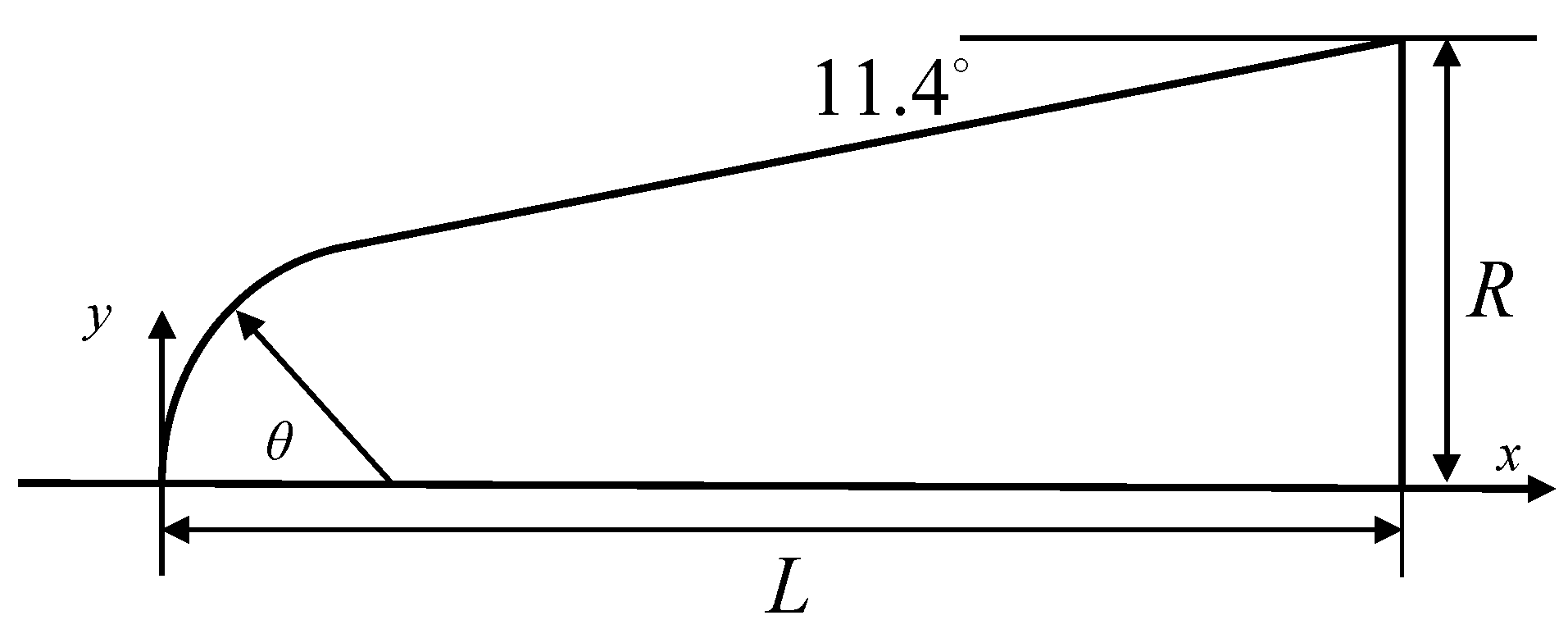
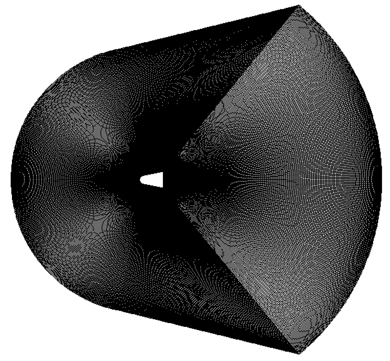
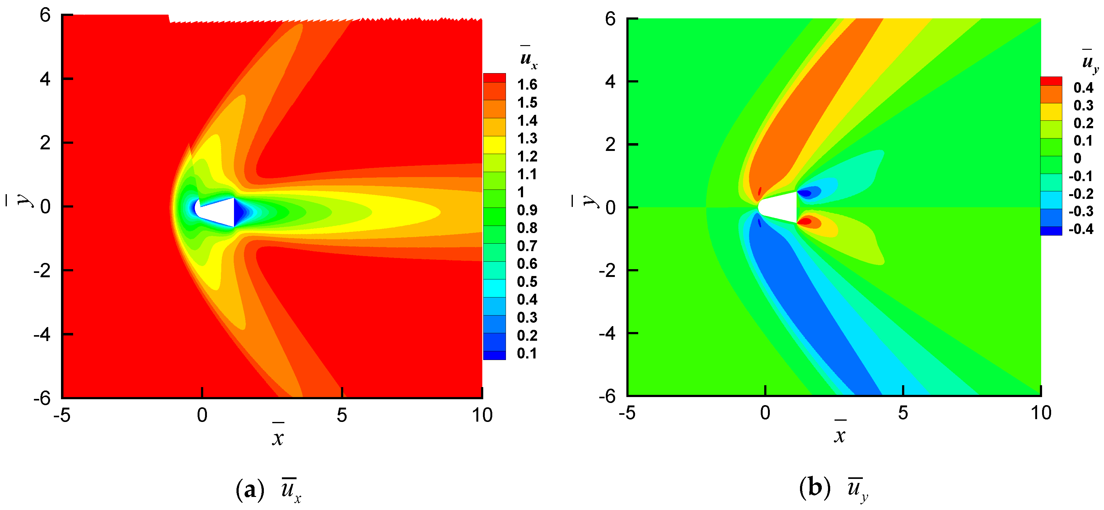
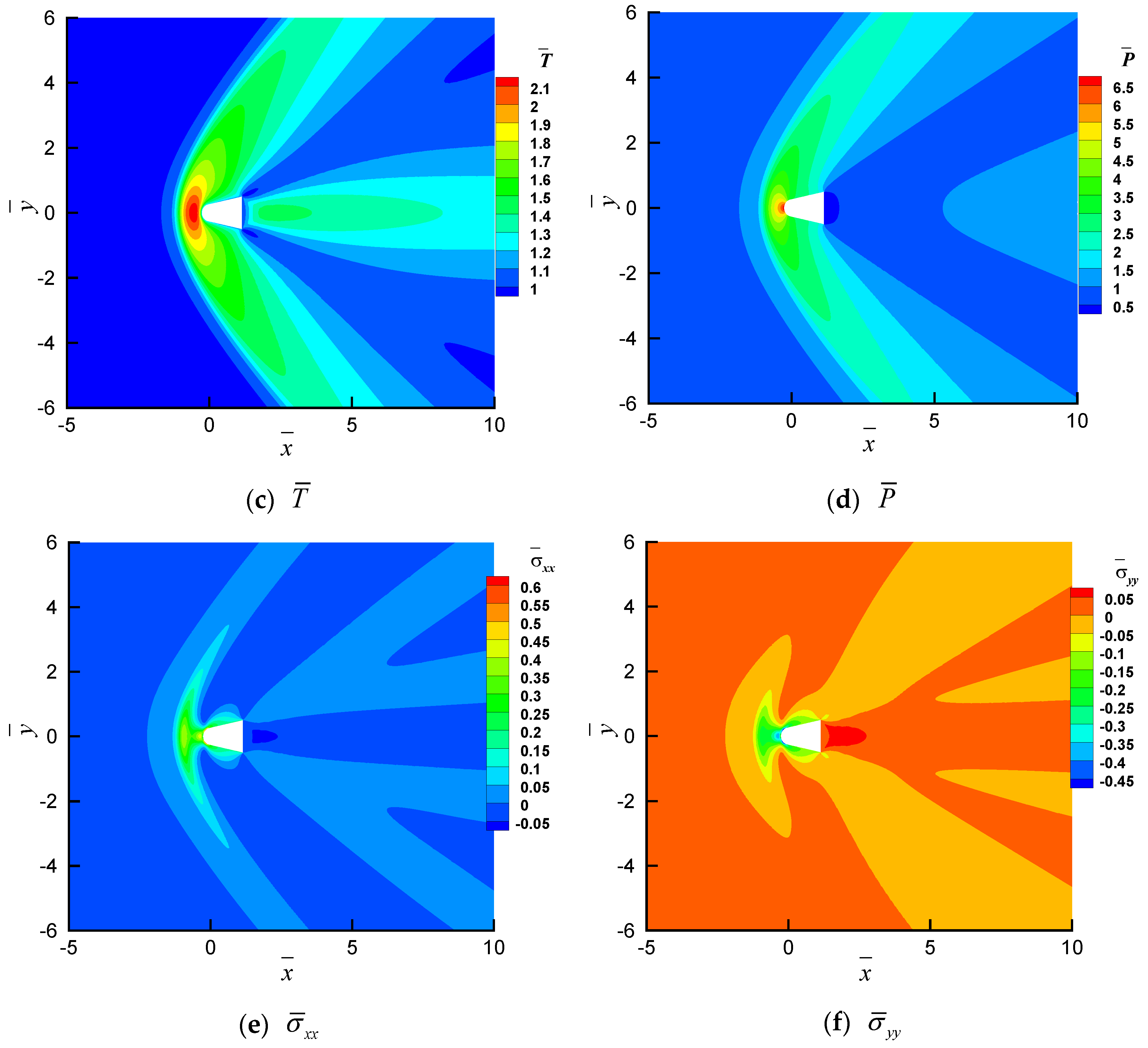
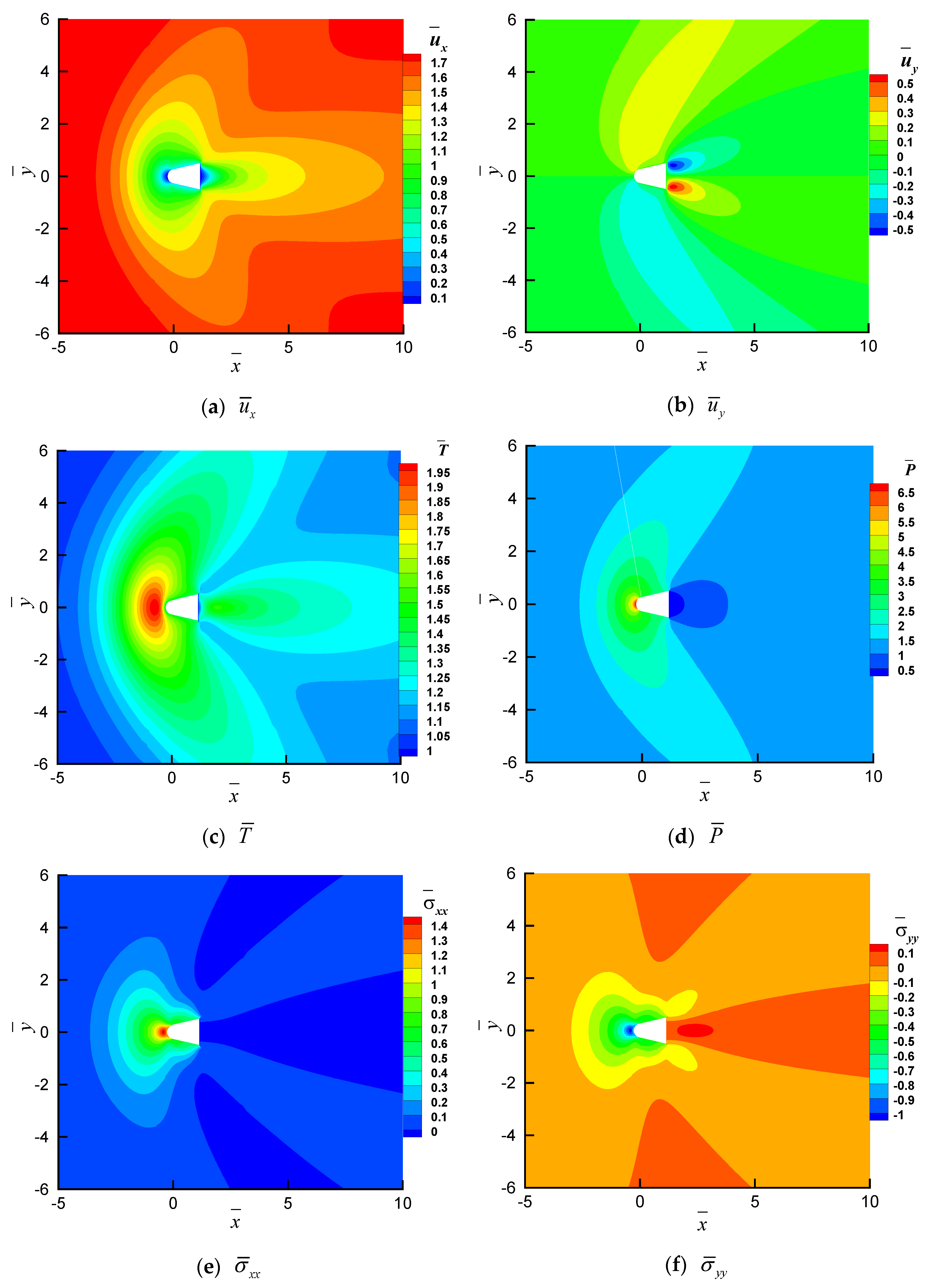
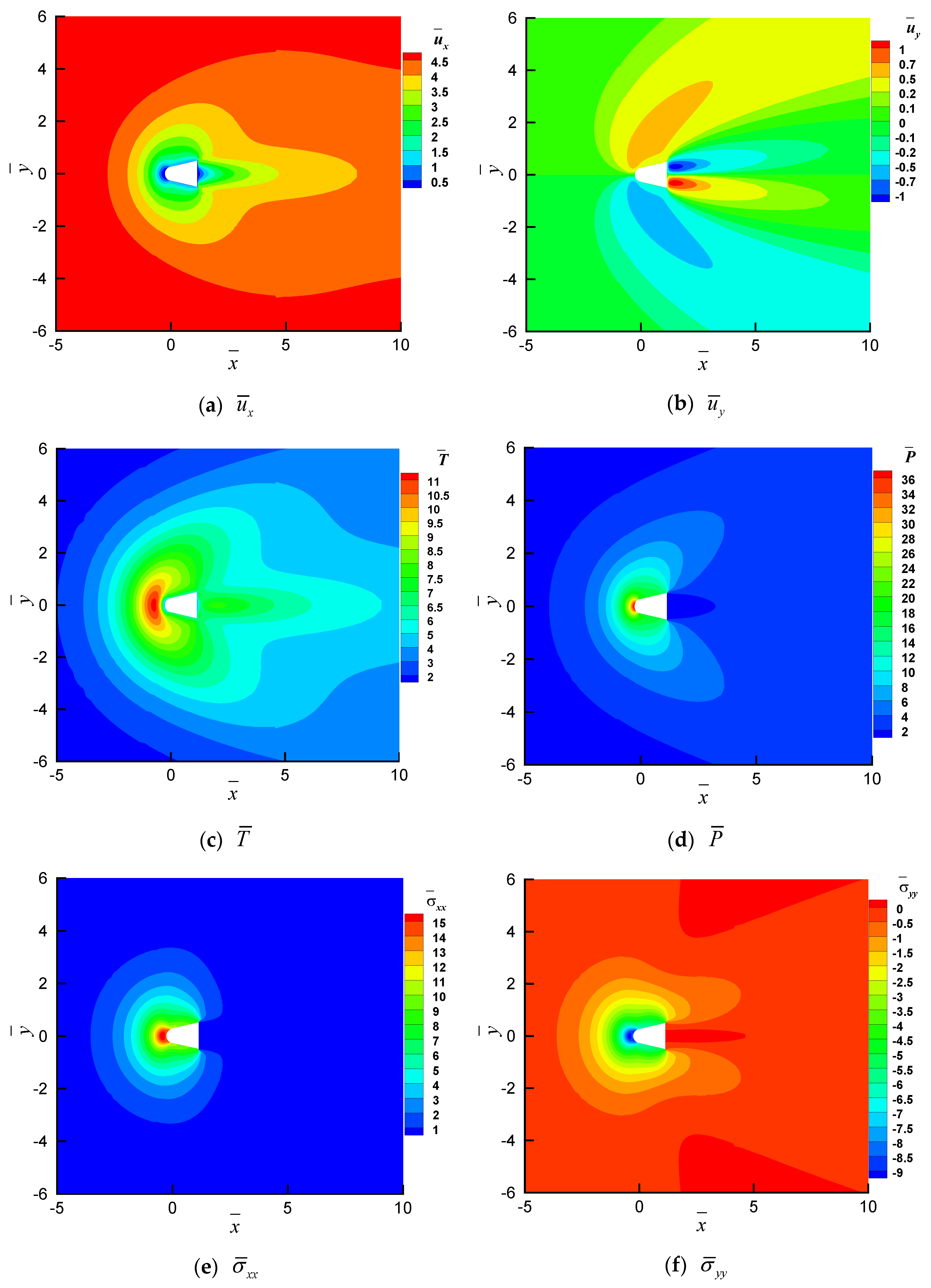
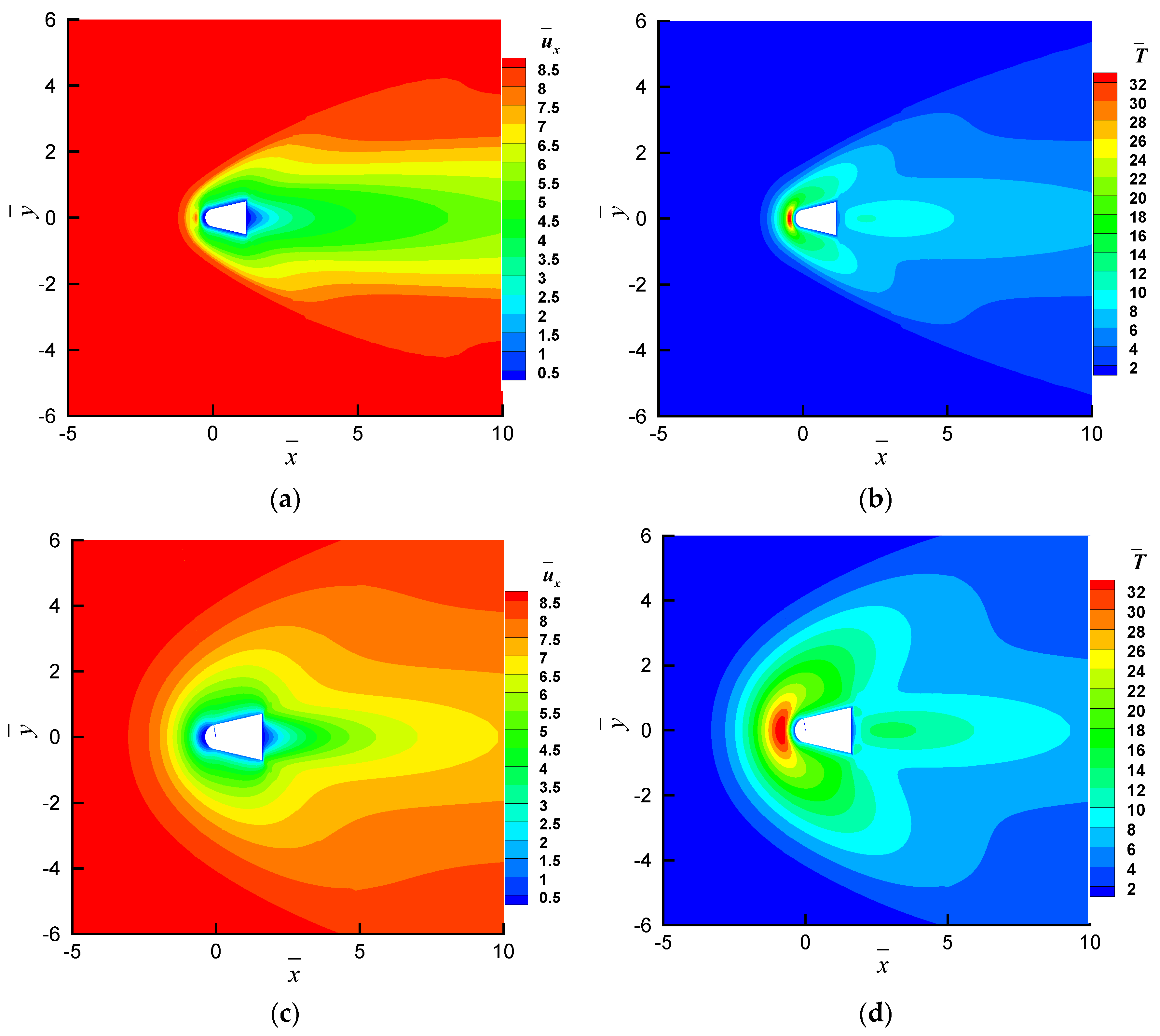
4.1. Gas Dynamics of a Cross-Domain Reentry Spheroid–Cone Unmanned Flight Vehicle

The geometry of the cross-domain reentry spheroid-cone unmanned flight vehicle is shown in Figure 2. The length and the bottom radius of the unmanned flight vehicle are L = 1.41   m and R = 0.5035   m , respectively, and R is the reference length. Since the model has some experimental and DSMC simulation data, the calculation accuracy of the algorithm can be verified.
In this study, the gas dynamics of the incoming flow with Ma = 2, 5, and 10 and Kn = 0.1 and 1 were studied. When Kn = 0.1 and 1.0, the flight height of the reentry vehicle was about 70–110 km, and the physical space was discretized with 90,000 and 10,000 non-uniform tetrahedral grids, respectively, as shown in Figure 3. The velocity space was discretized with 44 × 44 × 24 and 124 × 64 × 64 points, respectively. The independence of the results with respect to the discretization of molecular velocity and physical space was tested and confirmed [29]. The non-uniform Newton–Cotes quadrature can be defined as
C i = C max N 1 3 1 N + 2 i 3 , i = 0 , 1 , , N 1 ,
in which C max and N represent the maximum discrete velocity and the number of the discrete velocities, respectively. The numerical quadrature of the velocity distribution function can be defined as
Y = f C i d C i = 3 C max N 1 3 f C i a 2 d a .
Since a is in the form of an arithmetic sequence, the integral with respect to a can be computed using the trapezoidal rule or the Newton–Cotes formula. Normally, the more the discrete velocity points selected, the higher the computational accuracy that can be achieved, but the computational cost also increases accordingly.
The flow field parameters of the non-equilibrium rarefied gas flows past a cross-domain reentry unmanned flight vehicle at Ma = 2, Kn = 0.1 and Ma = 2, Kn = 1.0 are shown in Figure 4a–f and Figure 5a–f, respectively. When Ma = 2, 15 coupling layers are selected close to the wall of the spacecraft, and the ratios of the kinetic layers l to the reference length L 0 are l / L 0 = 0.89 for Kn = 0.1 and l / L 0 = 1.81 for Kn = 1.0, respectively. These coupling layers can produce accurate WBCs for the moment system.
The bow shock wave is clearly seen in front of the cone in Figure 4a, and the maximum dimensionless velocity u ¯ x = 1.6 and u ¯ y = 0 . 4 The maximum velocity appears in the expansion wave region on the upper right and lower right of the aircraft. Due to the strong shock compression, the temperature of the incoming flow rapidly rises when it approaches the front spherical vertebra of the aircraft, as shown in Figure 4c. Meanwhile, the pressure also rises rapidly with the compression of the air flow. The maximum dimensionless temperature and maximum dimensionless pressure are T ¯ = 2.1 ,   P ¯ = 6.5 , respectively. For Ma = 2, Kn = 0.1, the computational costs, in terms of computing memory and time, for the full DVM and the hybrid scheme are about 195.6 GB/1545 min and 3.84 GB/674 min, respectively.
Due to the non-equilibrium effect, it can be found from Figure 4a and Figure 5a that the greater the Kn number, the greater the thickness of the shock wave. In addition, it can also be found that the maximum dimensionless velocity appears further away from the surface of the aircraft. This is because when Kn = 1.0, the average free path between molecules is longer, the collision frequency and interaction between molecules are greatly reduced, and the impact of the aircraft wall on gas molecules is reduced. Therefore, the location of the expansion wave appears farther away from the wall compared with a small Kn. From Figure 5c,d, it can be seen that when Kn = 1.0, the change in the gas molecular temperature and pressure is not as drastic as that of low Knudsen numbers, which is also caused by a reduction in the number of collisions between molecules. The maximum temperature and maximum dimensionless pressure are about T ¯ = 1.95 ,   P ¯ = 6.5 .
The flow field parameters of the non-equilibrium rarefied gas flows past a cross-domain reentry unmanned flight vehicle, as the Ma number increases to 5.0, are shown in Figure 6a–f and Figure 7a–f. When Kn = 0.1, the strong shock structure can be clearly seen in front of the reentry flight vehicle, as shown in Figure 6a. When Kn is small and Ma = 5.0, the gas molecules are in the slip and early transition regimes. Hence, the compression effect of the shock wave is very strong, and the maximum dimensionless velocity is about u ¯ x = 4.5 . In addition, it can be observed that the expansion wave of the aircraft tail becomes less obvious as the Ma number increases to 5.0.
For the hypersonic incoming flows, the temperature and pressure increase sharply due to the compression effect, as shown in Figure 6c. The maximum temperature appears near the front of the flight vehicle, and the value of the dimensionless maximum temperature and pressure are about T ¯ = 11 and P ¯ = 36 , respectively. By comparing Figure 6a and Figure 7a, it can be observed that as the Kn increases, the shock layer at the head of the flight vehicle becomes thicker, and non-equilibrium effects become more critical for the aircraft.

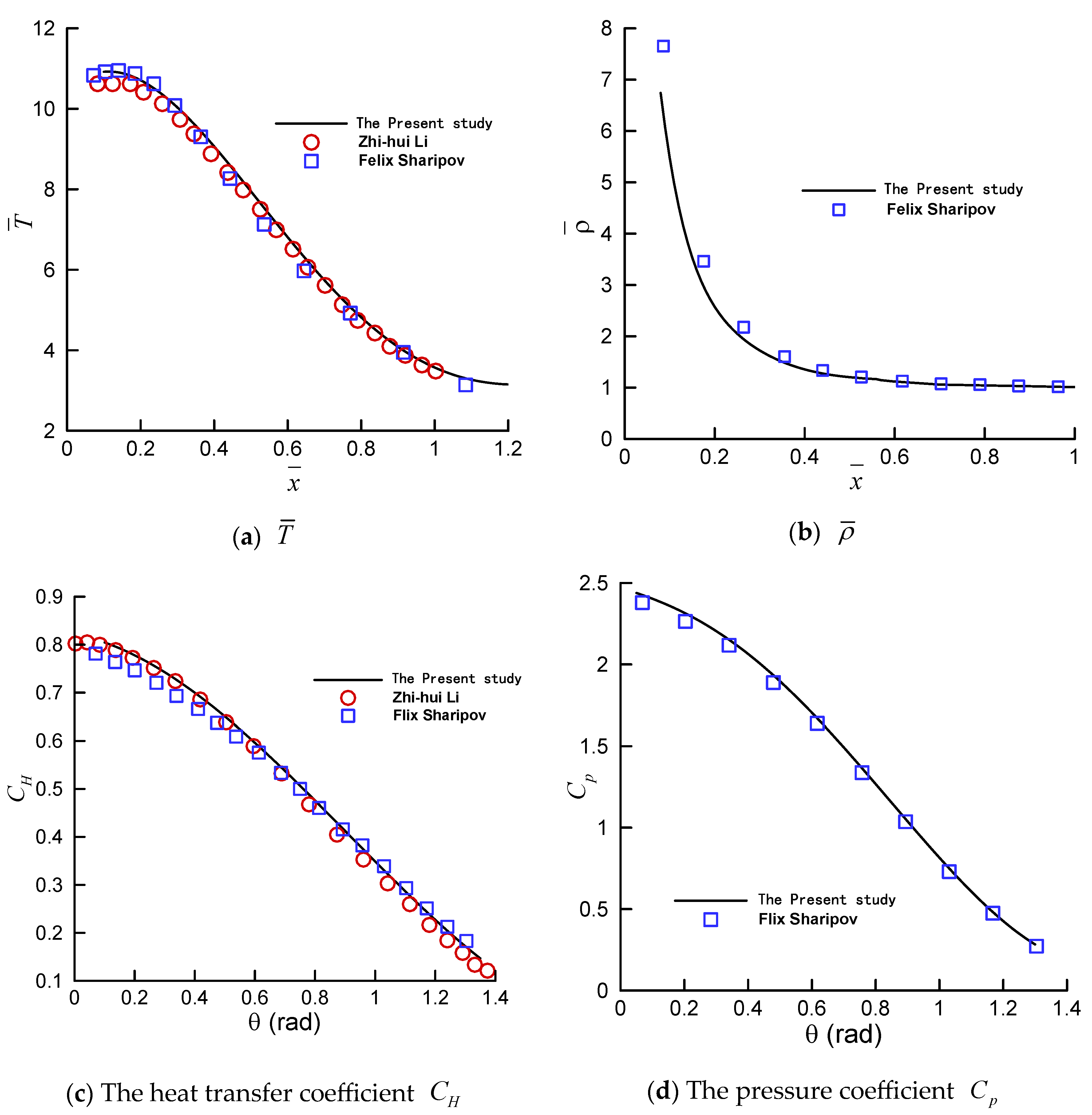
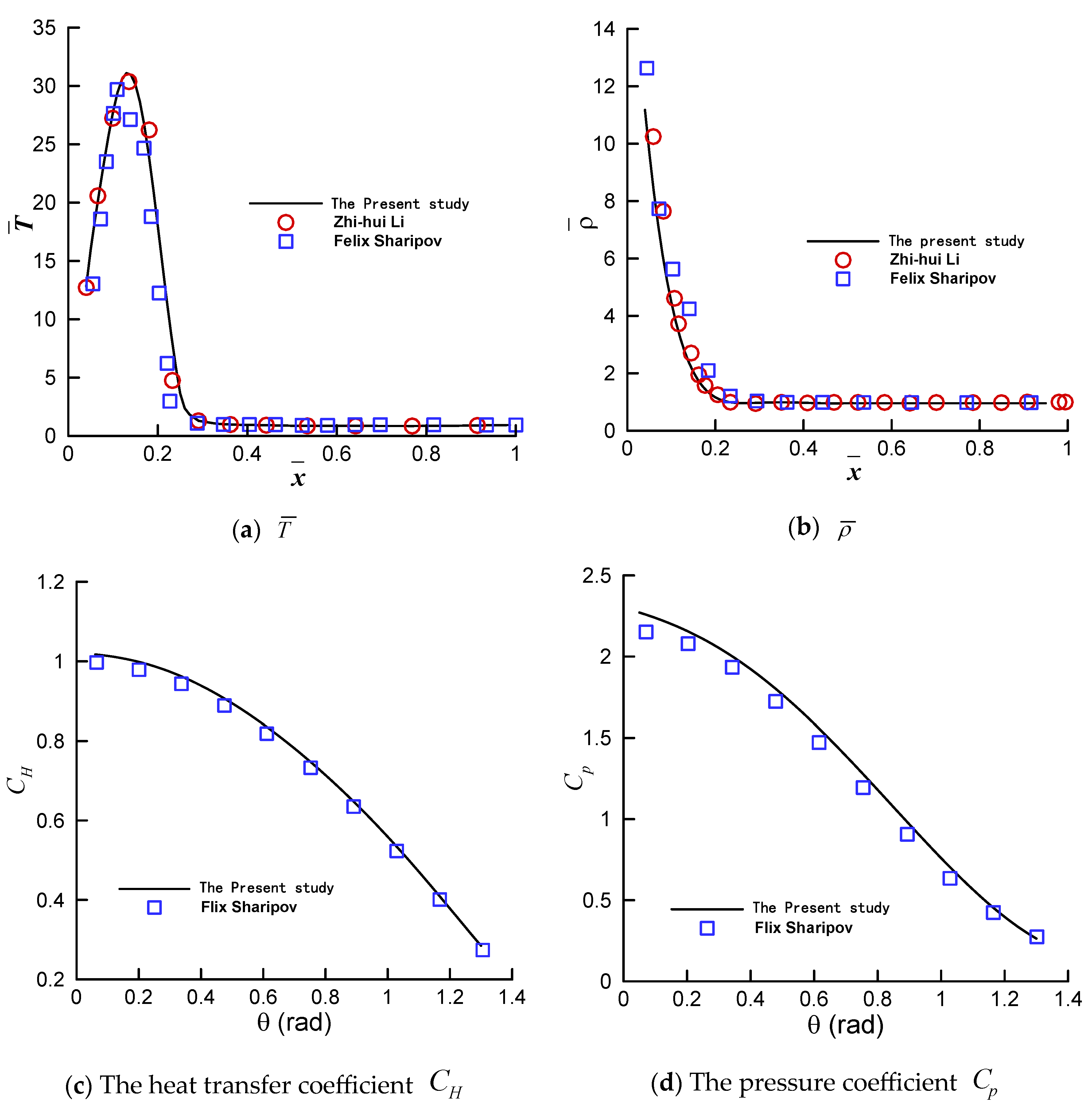
4.2. Comparison of the Computational Accuracy

The velocity, temperature, and density of the rarefied gas flows are represented by u ,   T ,   ρ , respectively. The Mach number Ma, Reynolds number Re, and Knudsen number Kn of the incoming flow can be expressed as follows:
(i)
The Ma number is defined as
M a = u c sound
in which c sound represents the speed of sound, which can be calculated as follows:
c s o u n d = γ k T m
in which k, m, and γ are the Boltzmann constant, molecular mass, and specific heat ratio, respectively.
(ii)
Re and Kn are defined as follows:
R e = R u ρ μ ,   K n = λ R
in which R and μ represent the radius of the bottom and the viscosity of the gas, respectively.
(iii)
The relationship between Re, Kn, and Ma is
K n = γ π 2 1 / 2 M a Re
(iv)
The pressure coefficient C P is expressed as follows:
C p = P P 1 / 2 ρ u 2
in which P and P represent the pressure of the aircraft and the pressure of the free flow, which follows the ideal gas law P = ρ R T .
(v)
The heat transfer coefficient C H is expressed as follows:
C H = q n 1 / 2 ρ u 2 u
where q n represents the heat flux perpendicular to the wall.
Figure 8a,b show the temperature T ¯ and pressure P ¯ distributions along the center line in front of the reentry flight vehicle at Ma = 5, Kn = 0.74, and these results were compared with those obtained by Zhi-hui Li [30] and Felix Sharipov [31]. Figure 8c,d show the pressure coefficient C P and the heat transfer coefficient C H on the surface of the reentry flight vehicle at Ma = 5. The maximum dimensionless temperature in front of the flight vehicle is T ¯ = 11.3 , and the temperature decreases rapidly within a reference length. Similarly, the maximum dimensionless density in front of the flight vehicle is ρ ¯ = 6 . 8 , and the calculated results in this study are in good agreement with the benchmark results.
From Figure 8c,d, the calculation results obtained in this study are consistent with those obtained by Zhi-hui Li and Felix Sharipov. The maximum errors of heat transfer coefficient and pressure coefficient are 2.1% and 3%, respectively. In Figure 8c, it is evident that the maximum heat transfer coefficient C H appears near the head of the aircraft, with a maximum value of C H = 0.82 . In addition, the heat transfer coefficient gradually decreases along the aircraft surface because the normal heat flow on the surface of the aircraft gradually decreases along the surface. In Figure 8d, the distribution of C P is similar to the change in the heat transfer coefficient C H , which reaches a maximum value of C P = 2.46 at the head of the aircraft and then gradually decreases along the surface.
With a further increase in the Ma number, i.e., Ma = 10.0, the non-equilibrium effect becomes significant, and more discrete velocities are needed to grasp the non-equilibrium effect. Hence, a mesh of 10,000 non-uniform tetrahedral elements was used to discretize the physical space, and 124 × 124 × 64 points were used to discretize the velocity space. The flow field parameters of the non-equilibrium flow past a cross-domain reentry unmanned flight vehicle at Ma = 10, Kn = 0.1 and Ma = 10, Kn = 1.0 are shown in Figure 9.
From Figure 9a, the curvature of the bow shock wave at Ma = 10.0 is greater than that of the low Mach numbers, and the expansion wave at the rear of the vehicle disappears. Meanwhile, it is clear to see from Figure 9a,c that as Kn increases, the thickness of the shock layer at the head of the flight vehicle becomes thicker, and non-equilibrium effects become more critical for the aircraft. The maximum velocities in the x and y directions are about u ¯ x = 8.5 and u ¯ y = 1.8 , respectively. Due to the shock wave, there is a strong heating effect in front of the cone, with a maximum dimensionless temperature and a maximum dimensionless pressure of T ¯ = 32 and P ¯ = 65 , respectively.
Figure 10a,b show the temperature T ¯ and pressure P ¯ distributions along the center line in front of the reentry flight vehicle at Ma = 10, and these results were compared with benchmark results. Figure 10c,d show the pressure coefficient C P and heat transfer coefficient C H of the surface of the reentry flight vehicle at Ma = 10.
It can be seen from Figure 10a that the temperature in front of the aircraft rapidly increases to T ¯ = 32 , and the maximum density is about ρ ¯ = 11 . The results obtained in this study are consistent with benchmark results, with a maximum density error of 9%. The maximum errors of the heat transfer coefficient and pressure coefficient are 2% and 4.6%, respectively. In addition, as the Mach number increases, the temperature and pressure ahead of the aircraft rise from T ¯ = 11 to T ¯ = 32 and from ρ ¯ = 6 . 8 to ρ ¯ = 11 , respectively. The maximum heat transfer coefficient C H and pressure coefficient C P appear at the head of the aircraft, with values of C H = 1.0 and C P = 2.23 , respectively.

5. Conclusions

A hybrid macro-/mesoscopic method is proposed for simulating rarefied gas flows past a cross-domain reentry unmanned flight vehicle in the present study. Gas dynamics of a typical cross-domain reentry spheroid–cone unmanned flight vehicle were investigated with different values of Kn and Ma, and the results were validated with those of Zhi-hui Li and Felix Sharipov. The simulation results showed that the hybrid macro-/mesoscopic scheme is well-suited for the non-equilibrium rarefied gas flows past a cross-domain reentry unmanned flight vehicle. Under the given conditions, the results obtained in this study are consistent with benchmark results, with a maximum density error of 9%. The maximum errors of the heat transfer coefficient and pressure coefficient were 2% and 4.6%, respectively. In addition, as the Knudsen number (Kn) becomes larger, the shock layer at the head of the flight vehicle becomes thicker, and non-equilibrium effects become more critical for the aircraft. Since the Boltzmann–Shakhov equation has only been solved close to the wall of a spacecraft, the computational cost can be considerably saved.

Author Contributions

W.Y. developed the code and performed the simulations. W.Y. analyzed the results and wrote the paper. J.M., B.X., H.D. and J.L. helped to revise the paper and analyze the results. All authors have read and agreed to the published version of the manuscript.

Funding

This research was funded by the National Natural Science Foundation of China (NSFC) under Grant Nos. 12302382 and 12372297 and the Hunan Provincial Natural Science Foundation of China under Grant No. 2022JJ40542.

Data Availability Statement

The original contributions presented in the study are included in the article, further inquiries can be directed to the corresponding author.

Acknowledgments

The authors would also like to thank X-J Gu (STFC Daresbury Laboratory, UK) for the useful discussions on the moment method and DVM.

Conflicts of Interest

The authors declare no conflicts of interest.

References

  1. Liang, Y.; Li, Z.; Jiang, X. The influence of reflected gas molecules state on flow characteristics at reentry condition. Flow Turbul. Combust. 2025. [Google Scholar] [CrossRef]
  2. Sun, J.; Zhu, H.; Han, H.; Xu, D.; Cai, G. Optimization of mechanical deployable reentry vehicle based on multi-fidelity aerodynamic-trajectory coupling model. Aerosp. Sci. Technol. 2025, 157, 109777. [Google Scholar]
  3. Yang, W.; Yang, H.; Tang, S. Optimization and control application of sensor placement in aeroservoelastic of UAV. Aerosp. Sci. Technol. 2019, 85, 61–74. [Google Scholar]
  4. Yang, W.; Gu, X.J.; Emerson, D.R.; Wu, L.; Zhang, Y.; Tang, S. A Hybrid Approach to Couple the Discrete Velocity Method and Method of Moments for Rarefied Gas Flows. J. Comput. Phys. 2020, 410, 109397. [Google Scholar]
  5. Yang, W.; Tang, S.; Yang, H. Analysis of the Moment method and the Discrete Velocity Method in Modeling Non-equilibrium Rarefied Gas Flows: A Comparative Study. Appl. Sci. 2019, 9, 2733. [Google Scholar] [CrossRef]
  6. Bird, G.A. Molecular Gas Dynamics and the Direct Simulation of Gas Flows; Clarendon Press: Oxford, UK, 1994; pp. 46–98. [Google Scholar]
  7. Goldstein, D.; Sturtevant, B.; Broadwell, J.E. Investigations of the motion of discrete-velocity gases. Prog. Astronaut. Aeronaut. 1989, 118, 100–117. [Google Scholar]
  8. Fang, M.; Li, Z.; Li, Z.; Liang, J.; Zhang, Y. DSMC modeling of rarefied ionization reactions and applications to hypervelocity spacecraft reentry flows. Adv. Aerodyn. 2020, 2, 7. [Google Scholar]
  9. Fang, M.; Li, Z.; Li, Z.; Li, C. DSMC Approach for Rarefied Air Ionization during Spacecraft Reentry. Commun. Comput. Phys. 2018, 23, 4. [Google Scholar]
  10. Bhatnagar, P.L.; Gross, E.P.; Krook, M. A model for collision processes in gases. I. Small amplitude processes in charged and neutral one-component systems. Phys. Rev. 1954, 94, 511–525. [Google Scholar]
  11. Holway, L.H., Jr. New statistical models for kinetic theory: Methods of construction. Phys. Fluids 1966, 9, 1658–1673. [Google Scholar]
  12. Shakhov, E. Generalization of the Krook kinetic relaxation equation. Fluid Dyn. 1968, 3, 95–96. [Google Scholar]
  13. Wu, L.; White, C.; Scanlon, T.J.; Reese, J.M.; Zhang, Y. Deterministic numerical solutions of the Boltzmann equation using the fast-spectral method. J. Comput. Phys. 2013, 250, 27–52. [Google Scholar]
  14. Li, Z.; Zhang, H. Gas-kinetic numerical studies of three-dimensional complex flows on spacecraft re-entry. J. Comput. Phys. 2009, 228, 1116–1138. [Google Scholar]
  15. Li, Z.; Liang, Y.; Peng, A.; Wu, J.; Wei, H. Gas-kinetic unified algorithm for aerodynamics covering various flow regimes by computable modeling of Boltzmann equation. Comput. Fluids 2025, 287, 106472. [Google Scholar]
  16. Li, F.; Li, Z.; Hu, J.; Hu, W. Application of gas-kinetic unified algorithm for solving Boltzmann model equation with vibrational energy excitation. Commun. Comput. Phys. 2025, 37, 250–288. [Google Scholar]
  17. Sone, Y. Flows induced by temperature fields in a rarefied gas and their ghost effect on the behavior of a gas in the continuum limit. Annu. Rev. Fluid Mech. 2000, 32, 779–811. [Google Scholar]
  18. Grad, H. On the kinetic theory of rarefied gases. Commun. Pure Appl. Math. 1949, 2, 331–407. [Google Scholar]
  19. Struchtrup, H.; Torrilhon, M. Regularization of Grad’s 13 moment equations: Derivation and linear analysis. Phys. Fluids 2003, 15, 2668–2680. [Google Scholar]
  20. Gu, X.-J.; Emerson, D.R. A computational strategy for the regularized 13 moment equations with enhanced wall-boundary conditions. J. Comput. Phys. 2007, 225, 263–283. [Google Scholar]
  21. Struchtrup, H.; Torrilhon, M. H Theorem, regularization and boundary conditions for linearized 13 moment equations. Phys. Rev. Lett. 2007, 99, 014502. [Google Scholar]
  22. Maxwell, J.C. On stresses in rarified gases arising from inequalities of temperature. Philos. Trans. R. Soc. Lond. A 1879, 170, 231–256. [Google Scholar]
  23. Gu, X.-J.; Emerson, D.R. A high-order moment approach for capturing non-equilibrium phenomena in the transition regime. J. Fluid Mech. 2009, 636, 177–216. [Google Scholar]
  24. Gu, X.-J.; Barber, R.W.; John, B.; Emerson, D.R. Non-equilibrium effects on flow past a circular cylinder in the slip and early transition regime. J. Fluid Mech. 2019, 860, 654–681. [Google Scholar]
  25. Gu, X.-J.; Emerson, D.R.; Tang, G.-H. Analysis of the slip coefficient and defect velocity in the Knudsen layer of a rarefied gas using the linearized moment equations. Phys. Rev. E 2010, 81, 016313. [Google Scholar]
  26. Yang, W.; Xu, B.; Niu, Y.; Zhou, Y. Thermally induced oscillatory rarefied gas flow inside a rectangular cavity. Phys. Fluids 2024, 36, 092033. [Google Scholar]
  27. Yang, W.; Gu, X.J.; Emerson, D.R.; Zhang, Y.; Tang, S. Modelling thermally induced non-equilibrium gas flows by coupling kinetic and extended thermodynamic methods. Entropy 2019, 21, 816. [Google Scholar] [CrossRef]
  28. Yang, W.; Gu, X.J.; Emerson, D.R.; Zhang, Y.; Tang, S. Comparative study of the discrete velocity and the moment method for rarefied gas flows. In Proceedings of the 31st International Symposium on Rarefied Gas Dynamics, Glasgow, UK, 23–28 July 2018; Volume 2132, p. 120006. [Google Scholar]
  29. Yang, W. Kinetic Theory and Applications of Rarefied Gas Flows Based on the Hybrid Discrete Velocity Method and Moment Method. Ph.D. Thesis, Northwestern Polytechnical University, Xi’an, China, 2019. (In Chinese). [Google Scholar]
  30. Li, Z.; Peng, A.; Zhang, H.; Yang, J. Rarefied gas flow simulations using high-order gas-kinetic unified algorithms for Boltzmann model equations. Prog. Aerosp. Sci. 2015, 74, 81–113. [Google Scholar]
  31. Sharipov, F. Hypersonic flow of rarefied gas near the Brazilian satellite during its reentry into atmosphere. Braz. J. Phys. 2003, 2, 398–405. [Google Scholar]
Figure 1. Configurational of the hybrid macro-/mesoscopic scheme.
Drones 09 00239 g001
Figure 2. Configurational parameters of the cross-domain reentry spheroid–cone unmanned flight vehicle.
Drones 09 00239 g002
Figure 3. Physical space grid of the cross-domain reentry flight vehicle.
Drones 09 00239 g003
Figure 4. The flow field parameters of the non-equilibrium rarefied gas flows past a cross-domain reentry unmanned flight vehicle at Ma = 2, Kn = 0.1. (a) Velocity, u ¯ x ; (b) velocity, u ¯ y ; (c) temperature, T ¯ ; (d) pressure, P ¯ ; (e) stress tensor, σ ¯ x x ; (f) stress tensor, σ ¯ y y .
Drones 09 00239 g004aDrones 09 00239 g004b
Figure 5. The flow field parameters of the non-equilibrium rarefied gas flows past a cross-domain reentry unmanned flight vehicle at Ma = 2, Kn = 1.0. (a) Velocity, u ¯ x ; (b) velocity, u ¯ y ; (c) temperature, T ¯ ; (d) pressure, P ¯ ; (e) stress tensor, σ ¯ x x ; (f) stress tensor, σ ¯ y y .
Drones 09 00239 g005
Figure 6. The flow field parameters of the non-equilibrium rarefied gas flows past a cross-domain reentry unmanned flight vehicle at Ma = 5, Kn = 0.1 (a) Velocity, u ¯ x ; (b) velocity, u ¯ y ; (c) temperature, T ¯ ; (d) pressure, P ¯ ; (e) stress tensor, σ ¯ x x ; (f) stress tensor, σ ¯ y y .
Drones 09 00239 g006
Figure 7. The flow field parameters of the non-equilibrium rarefied gas flows past a cross-domain reentry unmanned flight vehicle at Ma = 5, Kn = 1.0 (a) Velocity, u ¯ x ; (b) velocity, u ¯ y ; (c) temperature, T ¯ ; (d) pressure, P ¯ ; (e) stress tensor, σ ¯ x x ; (f) stress tensor, σ ¯ y y .
Drones 09 00239 g007
Figure 8. Flow parameters of the reentry flight vehicle. (a) Temperature, T ¯ ; (b) density, ρ ¯ ; (c) heat transfer coefficient, C H ; (d) pressure coefficient, C p , at Ma = 5, Kn = 0.74.
Drones 09 00239 g008
Figure 9. The flow field parameters of the non-equilibrium rarefied gas flows past a cross-domain reentry unmanned flight vehicle (a) u ¯ x at Ma = 10, Kn = 0.1; (b) T at Ma = 10, Kn = 0.1; (c) u ¯ x at Ma = 10, Kn = 1.0; (d) T at Ma = 10, Kn = 1.0.
Drones 09 00239 g009
Figure 10. Flow parameters of the reentry flight vehicle. (a) Temperature; (b) density; (c) heat transfer coefficient; (d) pressure coefficient, at Ma = 10, Kn = 0.004.
Drones 09 00239 g010
Table 1. Collision constants for the R26 moment scheme.
Notation A σ A q A m A R 1 , A R 2 A Δ 1 , A Δ 2 A ϕ 1 , A ϕ 2 A ψ 1 , A ψ 2 , A ψ 3 A Ω 1 , A Ω 2 , A Ω 3
Shakhov1Pr11,01,01,01,0,01,0,0
Disclaimer/Publisher’s Note: The statements, opinions and data contained in all publications are solely those of the individual author(s) and contributor(s) and not of MDPI and/or the editor(s). MDPI and/or the editor(s) disclaim responsibility for any injury to people or property resulting from any ideas, methods, instructions or products referred to in the content.

