A Robust Control Method for the Trajectory Tracking of Hypersonic Unmanned Flight Vehicles Based on Model Predictive Control

Abstract

Hypersonic unmanned flight vehicles have complex dynamic characteristics, such as nonlinearity, strong coupling, multiple constraints, and uncertainty. Operating in highly complex flight environments, hypersonic unmanned flight vehicles must not only contend with uncertainties and disturbances such as parameter perturbations and noise but also deal with complex task scenarios such as interception and no-fly zone avoidance. These factors collectively pose great challenges on the control performance of the vehicle. To address the challenges of trajectory tracking for the vehicles under complex constraints, this paper proposes a trajectory tracking control method based on model predictive control (MPC). Firstly, a nonlinear dynamic model for hypersonic unmanned flight vehicles is established. Then, a robust model predictive controller is designed and the optimal control law is derived to address the trajectory tracking control problem under complex constraints such as parameter perturbations. Finally, simulation experiments are designed under the conditions of aerodynamic parameter changes in the longitudinal plane and lateral no-fly zone avoidance. The simulation results demonstrate that the vehicle is capable of accurately and rapidly tracking the reference despite aerodynamic parameter perturbations and large-scale lateral maneuvers, thereby validating the effectiveness of the controller.

1. Introduction

Hypersonic flight vehicles have increasingly become a focal point of research in the aerospace field in recent years due to their advantages such as high speed, strong maneuverability, long range, and cost-effectiveness, offering broad application prospects in near-space [1]. However, compared to traditional aircraft, hypersonic flight vehicles operate in more complex flight environments and exhibit intricate aerodynamic characteristics, with a wide flight envelope and uncertain motion modeling. These factors result in the vehicles displaying characteristics such as multiple constraints, nonlinearity, strong coupling, and high uncertainty, posing significant difficulties and challenges for the study of their control technologies [2,3,4].

Traditional linear control methods often fall short in effectively addressing the complexity and unpredictability of hypersonic flight environments, making it difficult to achieve desired control performance. To realize the intended control objectives, many experts and scholars have applied various advanced control methods to hypersonic flight vehicles. Currently, advanced control methods employed in hypersonic flight vehicles include sliding mode control [5,6,7,8], adaptive control [9,10,11], backstepping control [12,13,14], active disturbance rejection control [15,16,17], and model predictive control [18,19,20]. Starting from a small speed ratio, Ref. [21] proposed a three-body cooperative active defense guidance law considering overload constraints. Based on a linearized cooperative guidance model, the guidance law was designed using the sliding mode control method to achieve active defense against incoming missiles. Ref. [22] proposed an innovative solution based on quadrotor motion control to address the issue of image motion blur caused by high-speed drone flight leading to detection failures. By actively adjusting the flight speed rather than relying on high-cost hardware or complex image post-processing techniques, this approach effectively mitigates the impact of motion blur on detection accuracy. Additionally, control methods integrating intelligent algorithms have been applied in the vehicle. For instance, Ref. [23] addressed the issue of actuator failures in quadrotor UAVs by proposing a hybrid control strategy based on reinforcement learning. This approach reduces computational complexity while enhancing real-time performance and ensuring the continuity of flight missions.

Model predictive control has gained widespread application in fields such as power, chemical engineering, and aerospace due to its low requirement for model precision, strong robustness and disturbance rejection capabilities, and its ability to effectively handle various system constraints. To address actuator saturation issues, a fault-tolerant control method based on MPC was designed in Ref. [24]; however, this method requires high-order derivatives of flight state variables, which are often difficult to obtain. For constraints such as combustion chamber temperature and pressure, a predictive controller based on a state-space model was designed in Ref. [25], achieving excellent tracking of height and velocity while effectively suppressing elastic mode vibrations. Regarding the re-entry guidance problem for hypersonic flight vehicles, Ref. [26] designed a feasible trajectory in the initial stage and achieved re-entry trajectory tracking by introducing model predictive control.

However, when applying predictive control methods to highly dynamic and fast time-varying systems like hypersonic flight vehicles, the complexity of online optimization calculations increases significantly. Since the control law must be optimized and solved at each step, the online computation time can be lengthy, potentially affecting the real-time performance of the vehicle control. To address this, many scholars have conducted exploratory research. In designing missile autopilots, Ref. [27] utilized the convex optimization tool CVXGEN to develop a control allocation method, enhancing the speed of MPC optimization calculations. Ref. [28] proposed a predictive functional control method based on a state-space model. By introducing basis functions and treating the control law as a linear combination of known basis functions, the dimensionality of solving the control law is reduced, achieving real-time control of hypersonic flight vehicles. Additionally, composite control methods that integrate model predictive control with other control strategies are gradually being applied to hypersonic flight vehicles. Ref. [29] comprehensively considered the amplitude of control inputs and velocity constraints, and combined neural networks with model predictive control to propose a new control method, which achieved optimal allocation of aerodynamic rudder commands. By integrating sliding mode control with predictive control, a predictive sliding mode control method [30,31,32] was developed, further enhancing the robustness of the controller. Ref. [33] proposed a tractable nonlinear robust model predictive control method, introducing an adaptive sliding mode into model predictive control to mitigate the impact of uncertainties in nonlinear systems. Ref. [34] combined MPC with LIDAR to address control problems in complex environments such as narrow tunnels and low-visibility conditions. They proposed a hierarchical architecture integrating MPC and SO(3), which significantly enhanced the system’s fault-tolerant capability. Therefore, compared to control methods such as sliding mode control and backstepping control, model predictive control is less demanding in terms of modeling accuracy and less reliant on precise models. This makes it particularly advantageous for hypersonic flight vehicles, which often involve unmodeled dynamics and highly complex systems.

In this paper, to address the trajectory tracking control problem of hypersonic flight vehicles under complex constraints, a trajectory tracking control method based on MPC is proposed. A hypersonic vehicle model and discrete state-space equations are established, and a robust model predictive controller is designed. Simulation experiments are conducted under the conditions of aerodynamic parameter changes in the longitudinal plane and lateral no-fly zone avoidance, respectively, validating the effectiveness of the controller. The main contributions are listed as follows:

(1)

Through combination with multi-step prediction and cyclic optimization mechanism on the basis of the dynamics model of hypersonic flight vehicles, an objective function optimization solution method is designed, and an MPC architecture suitable for trajectory tracking of the vehicle is constructed to ensure the flight stability of the vehicle under complex constraints.

(2)

The control law is adjusted by real-time feedback correction between the reference trajectory and system output through rolling optimization, effectively suppressing the impact of changes in aerodynamic parameters and exhibiting good robustness.

(3)

The MPC method is applied to lateral maneuver problems under no-fly zone constraints. Through its online adjustment mechanism, the vehicle achieves precise tracking of the reference trajectory. Compared to sliding mode control methods, MPC demonstrates higher accuracy in complex no-fly zone environments.

2. Dynamic Modeling and Problem Description

The equations used to describe hypersonic flight vehicles are numerous and the models are quite complex. Therefore, when studying related problems, simplifications are often made within acceptable accuracy limits. Generally, under certain assumptions, the motion of the vehicle is decomposed into longitudinal and lateral movements. This approach significantly reduces the number of equations that need to be solved simultaneously when analyzing the motion of the vehicle, making it easier to conduct further research.

The simplified models describing the longitudinal and lateral motion of the hypersonic flight vehicle flying at speeds exceeding Ma5 within the range of 20~100 km are shown as Equation (1) and Equation (2), respectively.

$$\left\{\begin{array}{l}\dot{h}=V\sin \theta \\ \dot{V}={\displaystyle \frac{P\cos \alpha -X}{m}}-g\sin \theta \\ \dot{\theta }={\displaystyle \frac{P\sin \alpha +Y}{mV}}-{\displaystyle \frac{g}{V}}\cos \theta \end{array}\right.$$

(1)

$$\left\{\begin{array}{l}\dot{h}=V\sin \theta \\ \dot{V}={\displaystyle \frac{P\cos \alpha -X}{m}}-g\sin \theta \\ V\dot{\theta }={\displaystyle \frac{P\sin \alpha +Y}{m}}\cos {\gamma }_s-{\displaystyle \frac{Z}{m}}\sin {\gamma }_s-g\cos \theta \\ -V\cos \theta {\dot{\psi }}_s={\displaystyle \frac{P\sin \alpha +Y}{m}}\sin {\gamma }_s+{\displaystyle \frac{Z}{m}}\cos {\gamma }_s\\ \dot{z}=-V\cos \theta \sin {\psi }_s\end{array}\right.$$

(2)

The meanings of the parameters in the model are shown in

Table 1. Meaning of each parameter in the model.

Parameter	Meaning	Parameter	Meaning
$h$	height	$P$	thrust
$V$	velocity	$X$	axial force
$\theta$	flight path angle	$Y$	normal force
${\psi }_s$	track yaw angle	$Z$	lateral force
$z$	lateral displacement	$\alpha$	angle of attack
$m$	mass	${\gamma }_s$	bank angle

.

And the aerodynamic model is as follows:

$$\left\{\begin{array}{l}X=C_{x}qS\\ Y=C_{y}qS\\ Z=C_{z}qS\\ q={\displaystyle \frac{1}{2}}\rho V^2\end{array}\right.$$

(3)

wherein $C_x,C_y,C_z$, respectively, represent the axial force coefficient, normal force coefficient, and lateral force coefficient; $S$ is the reference area of the vehicle; $\rho$ is the atmospheric density; and $q$ is dynamic pressure.

Since the scramjet engine generates thrust by compressing incoming air and mixing it with fuel for combustion at supersonic speeds, its thrust model can be expressed as follows [35]:

$$P=\varphi \cdot k\cdot I_{sp}\cdot f\left({\phi }_{inlet},\rho ,Ma,c,A\right)$$

(4)

specifically, the thrust $P$ is related to parameters such as specific impulse $I_{sp}$, equivalence ratio $\varphi$, proportionality coefficient $k$, inlet mass capture ratio ${\phi }_{inlet}$, inlet area $A$, Mach number $Ma$, atmospheric density $\rho$, and speed of sound $c$; $f\left(·\right)$ is a nonlinear function of $A,Ma,\rho ,c$, and its specific form can be found in Ref. [35].

From these equations, the mass capture ratio is highly coupled and exhibits strong nonlinearity with respect to parameters such as the angle of attack, sideslip angle, and Mach number. As a result, deriving an explicit state-space representation directly in terms of inputs like the angle of attack and equivalence ratio is highly non-trivial, rendering the design of a state-space-based controller particularly challenging. Moreover, although the model has been simplified by decoupling it into longitudinal and lateral dynamics, the model still reveals significant coupling among its parameters, complex flight mechanisms, and various uncertainties during operation, including parameter variations, actuator limitations, and no-fly zone avoidance. These factors pose significant challenges to controller design. Owing to its robustness to model inaccuracies and reduced reliance on precise modeling, model predictive control is well suited for systems with intricate and uncertain dynamics.

Therefore, it is of great significance to design a model-based controller, ensuring that the vehicle can accurately and stably track reference trajectories even in the presence of aerodynamic parameter variations or during extensive lateral maneuvers.

3. Design of Model Predictive Controller

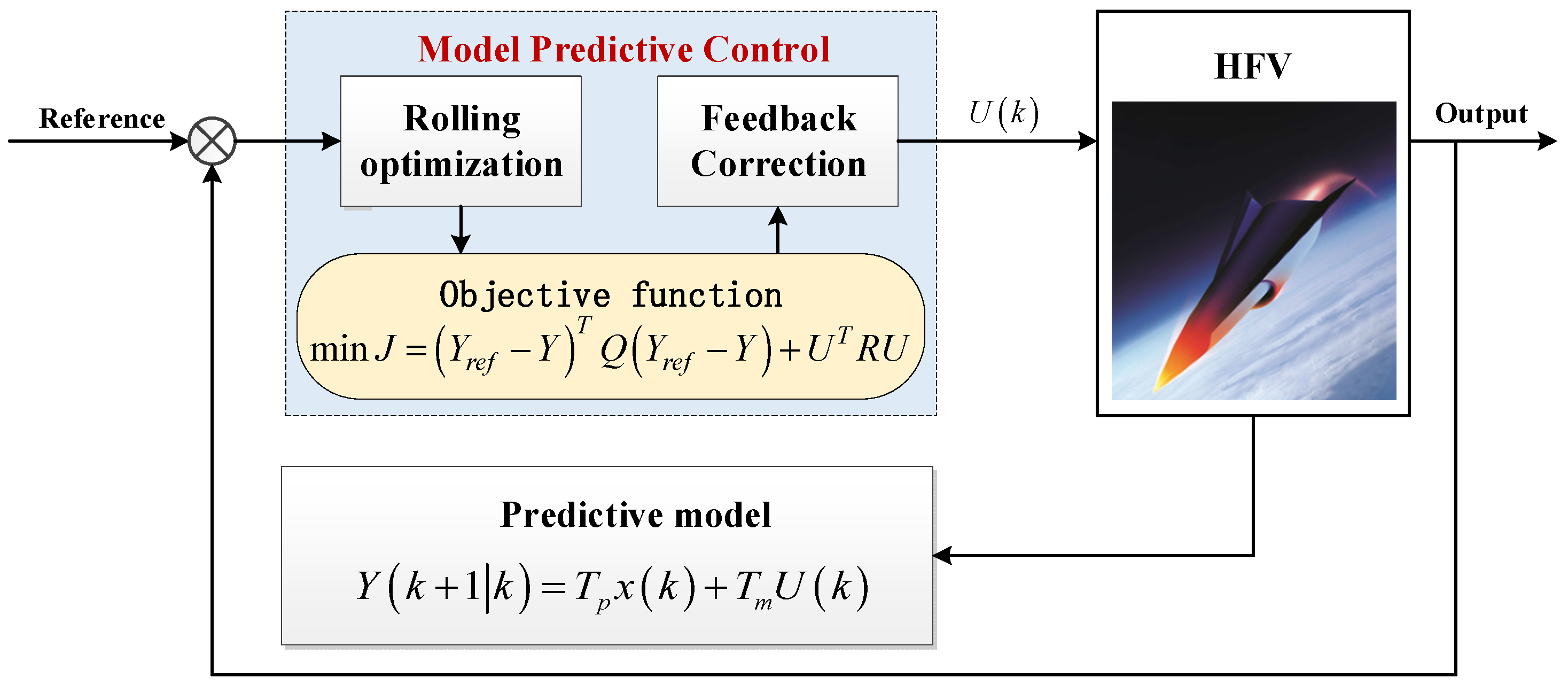
Considering the nonlinear and coupling characteristics of the vehicle in Equations (1)–(4), an MPC-based robust control strategy is proposed to ensure the precise and stable trajectory tracking of hypersonic flight vehicles under challenging conditions. Firstly, an MPC architecture suitable for trajectory tracking of the vehicle is constructed to ensure the flight stability of the vehicle, in which an objective function is designed in combination with the multi-step prediction and cyclic optimization mechanism. Then, the control law is derived by the rolling optimization and feedback correction between the reference trajectory and real-time output, effectively suppressing the impact of changes in aerodynamic parameters and exhibiting good robustness. Further, the control performance is demonstrated by using stability analysis and numerical simulation. The main structure of the proposed controller is illustrated in Figure 1.

3.1. Theory of Model Predictive Control

Model predictive control is fundamentally composed of three key components: predictive model, rolling optimization, and feedback correction. The core principle can be summarized as, at each sampling instant, taking the current state of the system as the initial condition and utilizing the mathematical model of the system to predict the future behavior of the controlled process over a finite prediction horizon. By optimizing the performance index, the optimal control input sequence is solved. The first element of this control sequence is then applied to the system, with corrections made based on actual feedback. This closed-loop process is reiterated at each subsequent sampling instant, ensuring robustness and adaptability in dynamic environments.

The linear controlled system can be represented in the following form:

$$\left\{\begin{array}{l}x\left(k+1\right)=Ax\left(k\right)+Bu\left(k\right)\\ y\left(k\right)=Cx\left(k\right)\end{array}\right.$$

(5)

where $x\left(k\right)$ is the state variable, $y\left(k\right)$ is the output variable, $u\left(k\right)$ is the control input variable, $A$ is the state matrix, $B$ is the control input matrix, and $C$ is the coefficient matrix of the output, without considering the interference term.

Taking time instant $k$ as the starting point for predicting the future dynamics of the system, with a prediction horizon of $p$ and a control horizon of $m$, the predictions span from step 1 to step $p$, while the control actions are implemented over $m$ steps:

$$\begin{array}{ccc}\hfill x\left(k+1\left|k\right.\right)& =& Ax\left(k\right)+Bu\left(k\right)\hfill \\ \hfill x\left(k+2\left|k\right.\right)& =& A^{2}x\left(k\right)+ABu\left(k\right)+Bu\left(k+1\right)\hfill \\ & ⋮& \\ \hfill x\left(k+p\left|k\right.\right)& =& A^{p}x\left(k\right)+A^{p-1}Bu\left(k\right)+\cdots A^{p-m}Bu\left(k+m-1\right)\hfill \\ & +& ABu\left(k+m-1\right)+Bu\left(k+m-1\right)\hfill \end{array}$$

(6)

Then, the output equation is

$$\begin{array}{ccc}\hfill y\left(k+1\left|k\right.\right)& =& CAx\left(k\right)+CBu\left(k\right)\hfill \\ \hfill y\left(k+2\left|k\right.\right)& =& C{A}^{2}x\left(k\right)+CABu\left(k\right)+CBu\left(k+1\right)\hfill \\ & ⋮& \\ \hfill y\left(k+p\left|k\right.\right)& =& C{A}^{p}x\left(k\right)+C{A}^{p-1}Bu\left(k\right)+\cdots +C{A}^{p-m}Bu\left(k+m-1\right)\hfill \\ & +& CABu\left(k+m-1\right)+CBu\left(k+m-1\right)\hfill \end{array}$$

(7)

Define the output prediction vector and input control vector as follows:

$$Y={\left[y\left(k+1\left|k\right.\right),y\left(k+2\left|k\right.\right),\cdots ,y\left(k+p\left|k\right.\right)\right]}^T$$

(8)

$$U={\left[u\left(k\right),u\left(k+1\right),\cdots ,u\left(k+m-1\right)\right]}^T$$

(9)

The predicted output equation can be written as

$$Y\left(k+1\left|k\right.\right)=T_{p}x\left(k\right)+T_{m}U\left(k\right)$$

(10)

where

$$T_p=\left[\begin{array}{c}CA\\ ⋮\\ C{A}^m\\ C{A}^{m+1}\\ ⋮\\ C{A}^p\end{array}\right],T_m=\left[\begin{array}{ccc}CB& \cdots & 0\\ ⋮& \cdots & ⋮\\ C{A}^{m-1}B& \cdots & CB\\ C{A}^{m}B& \cdots & CAB+CB\\ ⋮& \cdots & ⋮\\ C{A}^{p-1}B& \cdots & {\displaystyle \sum _{i=0}^{p-m}C{A}^{i}B}\end{array}\right]$$

Design the following objective function to solve the optimal control input sequence:

$$J={\left(R_s-Y\right)}^{T}Q\left(R_s-Y\right)+U^{T}RU$$

(11)

where $R_s$ represents the desired output value at time instant $k$, and $Q$ and $R$ are the corresponding weighting coefficient matrices, respectively.

Substituting Equation (10) into Equation (11) yields

$$J={\left[R_s-T_{p}x\left(k\right)\right]}^{T}Q\left[R_s-T_{p}x\left(k\right)\right]-2U^T{T}_m^{T}Q\left[R_s-T_{p}x\left(k\right)\right]+U^T\left(T_m^{T}Q{T}_m+R\right)U$$

(12)

Thus, the control problem is formulated as an optimization problem of the objective function, which is shown as follows:

$$\min J={\left(R_s-Y\right)}^{T}Q\left(R_s-Y\right)+U^{T}RU$$

(13)

By employing the least squares method or an optimization algorithm to solve Equation (13) within the prediction horizon, the optimal control input sequence can be obtained. For this sequence, the first element is taken as the control input at the current time, which is applied to the controlled system to obtain the predicted output for the next moment. On this basis, rolling optimization over a finite time horizon is continuously performed, the predictive model is refined, and the optimal control law is calculated, thereby enhancing the accuracy of the predictions.

3.2. Design of the MPC-Based Control Strategy

Nonlinear model predictive control is an extension of the aforementioned linear model predictive control, with its governing equations composed of a set of nonlinear differential equations. For a nonlinear model, it can be represented in the following form:

$$\left\{\begin{array}{l}x\left(k+1\right)=g\left(x\left(k\right),u\left(k\right)\right)\\ y\left(k\right)=h\left(x\left(k\right)\right)\end{array}\right.$$

(14)

Discretizing Equation (1), which represents the longitudinal dynamics model of the hypersonic vehicle, can obtain the discretized state equations:

$$\left\{\begin{array}{l}h\left(k+1\right)=h\left(k\right)+TV\left(k\right)\sin \left(\theta \left(k\right)\right)\\ V\left(k+1\right)=V\left(k\right)+T\left(\left(P\cos \alpha -X\right)/m-g\sin \left(\theta \left(k\right)\right)\right)\\ \theta \left(k+1\right)=\theta \left(k\right)+T\left(\left(P\sin \alpha +Y\right)/\left(mV\left(k\right)\right)-g\cos \left(\theta \left(k\right)\right)/V\left(k\right)\right)\end{array}\right.$$

(15)

where $x\left(k\right)={\left[h\left(k\right),V\left(k\right),\theta \left(k\right)\right]}^T$ is the state variable, $u\left(k\right)={\left[\alpha \left(k\right),\varphi \left(k\right)\right]}^T$ is the control input variable, $\varphi$ is the equivalence ratio used to calculate thrust, and $T$ is the sampling interval time.

For this discrete state equation, write it in the form of Equation (14):

$$\left\{\begin{array}{l}x\left(k+1\right)=g_1\left(x\left(k\right),u\left(k\right)\right)\\ y\left(k\right)=h_1\left(x\left(k\right)\right)\end{array}\right.$$

(16)

Starting from the state $x\left(k\right)$ at current time step $k$, the future state sequence is computed through $p$ step prediction and $m$ step control, which can be expressed as follows:

$$\begin{array}{ccc}\hfill x\left(k+1\left|k\right.\right)& =& g_1\left(x\left(k\right),u\left(k\right)\right)\hfill \\ \hfill x\left(k+2\left|k\right.\right)& =& g_1\left(x\left(k+1\right),u\left(k+1\right)\right)\hfill \\ & ⋮& \\ \hfill x\left(k+p\left|k\right.\right)& =& g_1\left(x\left(k+p-1\right),u\left(k+m-1\right)\right)\hfill \end{array}$$

(17)

The corresponding model output is

$$\begin{array}{ccc}\hfill y\left(k+1\left|k\right.\right)& =& h_1\left(x\left(k+1\left|k\right.\right)\right)\hfill \\ \hfill y\left(k+2\left|k\right.\right)& =& h_1\left(x\left(k+2\left|k\right.\right)\right)\hfill \\ & ⋮& \\ \hfill y\left(k+p\left|k\right.\right)& =& h_1\left(x\left(k+p\left|k\right.\right)\right)\hfill \end{array}$$

(18)

Set the following objective function:

$$J={\left(Y_{ref}-Y_k\right)}^{T}Q\left(Y_{ref}-Y_k\right)+{U_k}^{T}R{U}_k$$

(19)

where $Y_k=\left[y\left(k+1\right),y\left(k+2\right),\cdots ,y\left(k+p\right)\right]$ is the predicted output, $Y_{ref}$ is the reference value for the corresponding variable, and $U_k=\left[u\left(k\right),u\left(k+1\right),\cdots ,u\left(k+m-1\right)\right]$ is the control input.

The control constraint is

$$U_{\min }\le U_k\le U_{\max }$$

(20)

Minimize Equation (19) while satisfying the constraints, i.e.,

$$\min J={\left(Y_{ref}-Y_k\right)}^{T}Q\left(Y_{ref}-Y_k\right)+{U_k}^{T}R{U}_k$$

(21)

$$s.t.\left\{\begin{array}{l}x\left(k+1\right)=g\left(x\left(k\right),u\left(k\right)\right)\\ y\left(k+1\right)=h\left(x\left(k+1\right)\right)\\ U_{\min }\le U_k\le U_{\max }\end{array}\right.$$

(22)

To solve the optimization problem, the Sequential Quadratic Programming (SQP) method is employed. For computational convenience, the optimization problem is further transformed into

$$\min J={\Gamma }_1\left(U_k\right)$$

(23)

$$U_k-U_{\min }\ge 0,U_k-U_{\max }\le 0$$

(24)

where ${\Gamma }_1\left(U_k\right)={\left(Y_{ref}-Y_k\right)}^{T}Q\left(Y_{ref}-Y_k\right)+{U_k}^{T}R{U}_k$.

By performing a Taylor expansion of the optimization problem at the iteration point $U_k$, the following quadratic programming subproblem is obtained:

$$\begin{array}{cc}\hfill \min {\Gamma }_1\left(U_k\right)& =\nabla {\Gamma }_1{\left(U_k\right)}^T\left[U-U_k\right]+{\displaystyle \frac{1}{2}}{\left[U-U_k\right]}^T{\nabla }^2{\Gamma }_1\left(U_k\right)\left[U-U_k\right]\hfill \\ \hfill s.t.L& \le U-U_k\le R\hfill \end{array}$$

(25)

where $L=U_{\min }-U_k,R=U_{\max }-U_k$.

Equation (25) is merely an approximation of the original problem, and the solution obtained is only a local optimum rather than the global optimum of the original problem. Therefore, let

$$d=U-U_k$$

(26)

$$C=\nabla {\Gamma }_1\left(U_k\right)$$

(27)

$$H_k={\nabla }^2{\Gamma }_1\left(U_k\right)$$

(28)

Then, Equation (25) is

$$\begin{array}{c}\min {\Gamma }_1\left(U_k\right)=C^{T}d+{\displaystyle \frac{1}{2}}{d}^T{H}_{k}d\\ s.t.L\le d\le R\end{array}$$

(29)

By introducing Lagrange multipliers $\lambda$ and $\mu$, the Lagrange function is constructed as follows:

$$L\left(U,\lambda ,\mu \right)={\Gamma }_1\left(U\right)-{\lambda }^T\left(U-U_{\min }\right)-{\mu }^T\left(U_{\max }-U\right)$$

(30)

The KKT condition for solving QP subproblems is

$$\left\{\begin{array}{l}{H}_{k}d+\nabla {\Gamma }_k-\lambda +\mu =0;\\ {\lambda }_i\left(d_i-L_i\right)=0,{\mu }_i\left(R_i-d_i\right)=0;\\ \lambda \ge 0,\mu \ge 0.\end{array}\right.$$

(31)

Solve the QP subproblem to obtain $d_k$, and update variables and multipliers:

$$U_{k+1}=U_k+{\alpha }_k{d}_k$$

(32)

$${\lambda }_{k+1}={\lambda }_k+{\alpha }_k\left({\lambda }_k^{*}-{\lambda }_k\right)$$

(33)

$${\mu }_{k+1}={\mu }_k+{\alpha }_k\left({\mu }_k^{*}-{\mu }_k\right)$$

(34)

where ${\lambda }_k^{*}$ and ${\mu }_k^{*}$ are the solutions to the quadratic programming subproblem, while ${\alpha }_k\in \left(0,\left.1\right]\right.$ is determined through a line search to ensure the objective function decreases and the constraints are satisfied. This iterative process is repeated until the convergence criteria are met, yielding the optimal solution to the original problem. Subsequently, the first element of the optimal control input sequence is selected as the control input for the current moment, and the output for the next moment is predicted. Through continuous rolling optimization, the optimal control law is calculated.

Similarly, for the lateral maneuvering model, its discretized state equation is

$$\left\{\begin{array}{cc}\hfill h\left(k+1\right)& =h\left(k\right)+TV\left(k\right)\sin \left(\theta \left(k\right)\right)\hfill \\ \hfill V\left(k+1\right)& =V\left(k\right)+T\left(u_1-g\sin \left(\theta \left(k\right)\right)\right)\hfill \\ \hfill \theta \left(k+1\right)& =\theta \left(k\right)+T\left(u_2\cos {\gamma }_s/V\left(k\right)\right)-\hfill \\ & T\left(Z\sin {\gamma }_s/mV\left(k\right)\right)-T\left(g\cos \left(\theta \left(k\right)\right)/V\left(k\right)\right)\hfill \\ \hfill {\psi }_s\left(k+1\right)& ={\psi }_s\left(k\right)-T\left(u_2\sin {\gamma }_s/V\left(k\right)\cos \left(\theta \left(k\right)\right)\right)\hfill \\ & -T\left(Z\cos {\gamma }_s/mV\left(k\right)\cos \left(\theta \left(k\right)\right)\right)\hfill \\ \hfill z\left(k+1\right)& =z\left(k\right)+T\left(-V\left(k\right)\cos \left(\theta \left(k\right)\right)\sin \left({\psi }_s\left(k\right)\right)\right)\hfill \end{array}\right.$$

(35)

The prediction model obtained based on this equation is

$$\left\{\begin{array}{l}x\left(k+1\right)=g_2\left(x\left(k\right),u\left(k\right)\right)\\ y\left(k\right)=h_2\left(x\left(k\right)\right)\end{array}\right.$$

(36)

where $x\left(k\right)={\left[h\left(k\right),V\left(k\right),\theta \left(k\right),{\psi }_s\left(k\right),z\left(k\right)\right]}^T$ is the state variable, and $u\left(k\right)={\left[\alpha \left(k\right),\varphi \left(k\right)\right]}^T$ is the control input.

Similarly to the approach for longitudinal issues, it can be transformed into the optimization problem as shown in Equations (37) and (38).

$$\min J={\Gamma }_2\left(U_k\right)$$

(37)

$$U_k-U_{\min }\ge 0,U_k-U_{\max }\le 0$$

(38)

The optimal solution is computed utilizing the SQP algorithm, where the first element of the optimal control input sequence is adopted as the control input for the current time step. Subsequently, the output for the next time step is predicted, and the process undergoes continuous receding horizon optimization to derive the optimal control law for lateral maneuvering.

3.3. Stability Analysis

Furthermore, to prove the stability of the proposed control strategy, the terminal cost function $V_f\left(x_{k+p}\right)$ and terminal constraint set ${\chi }_f$ are introduced and satisfy the following:

$$V_f\left(f\left(x_{k+p},u_{k+p}\right)\right)-V_f\left(f\left(x_{k+p}\right)\right)\le -l\left(x_{k+p},u_{k+p}\right)$$

(39)

where $l\left(x,u\right)={‖x-x_{ref}‖}_Q^2+{‖u-u_{ref}‖}_R^2,x_{k+p}\in {\chi }_f$.

For optimization problem (23), the constructed function is

$$J\left(x_k,u\right)={\displaystyle \sum _{i=0}^{p-1}l\left(x_{k+i},u_{k+i}\right)}+V_f\left(x_{k+p}\right)$$

(40)

Assuming the optimization problem is feasible at the initial time instant, it needs to be proven that the problem remains feasible at the next time instant. Let the optimal control sequence at time step $k$ be denoted as $\left\{u_k^{*},u_{k+1}^{*},\cdots ,u_{k+p-1}^{*}\right\}$, with the corresponding terminal state being $x_{k+p}\in {\chi }_f$.

At the time step $k+1$, a new sequence $\left\{u_{k+1}^{*},\cdots ,u_{k+p-1}^{*},u^{\prime }\right\}$ is constructed, where $u^{\prime }$ is derived from $f\left(x_{k+p}^{*},u^{\prime }\right)\in {\chi }_f$, ensuring that the terminal state $x_{k+p+1}^{\prime }=f\left(x_{k+p}^{*},u^{\prime }\right)\in {\chi }_f$ satisfies the feasibility.

Define the Lyapunov function as the objective function and prove its monotonic decrease:

$$V^{*}\left(x_k\right)=\min J\left(x_k,u\right)$$

(41)

At time step $k+1$, the optimal value is $V^{*}\left(x_{k+1}\right)$, and based on the constructed feasible sequence, it satisfies the following equation:

$$J\left(x_{k+1},u^{\prime }\right)=V^{*}\left(x_k\right)-l\left(x_k,u_k^{*}\right)+\left[V_f\left(f\left(x_{k+p}^{*},u^{\prime }\right)\right)-V_f\left(x_{k+p}^{*}\right)+l\left(x_{k+p}^{*},u^{\prime }\right)\right]$$

(42)

From the terminal constraint $V_f\left(f\left(x_{k+p}^{*},u^{\prime }\right)\right)\le V_f\left(x_{k+p}^{*}\right)-l\left(x_{k+p}^{*},u^{\prime }\right)$, it follows that

$$J\left(x_{k+1},u^{\prime }\right)\le V^{*}\left(x_k\right)-l\left(x_k,u_k^{*}\right)$$

(43)

Since $V^{*}\left(x_{k+1}\right)\le J\left(x_{k+1},u^{\prime }\right)$, it follows that

$$V^{*}\left(x_{k+1}\right)\le V^{*}\left(x_k\right)-l\left(x_k,u_k^{*}\right)$$

(44)

This shows that $V^{*}$ decreases monotonically and $l\left(x_k,u_k^{*}\right)\to 0$, thereby $x_k\to 0$, which guarantees the asymptotic stability of the system.

The process of proving stability is similar to that of proving longitudinal problems.

4. Simulation Analysis

To demonstrate the effectiveness of the designed controller, simulations are conducted under two scenarios: variations in aerodynamic parameters in the longitudinal plane and lateral maneuvers for no-fly zone avoidance. The outcomes are detailed below.

4.1. Verification of Longitudinal Simulation

The vehicle accelerates into steady-state cruising from the initial point of [20 km, Ma5] in the longitudinal plane. When accelerating to the cruising Mach number, the control variables adjust to mitigate aerodynamic disturbances and stabilize the velocity and height. A reference trajectory is subsequently generated with the optimization goal of minimizing fuel consumption. After obtaining the reference trajectory, the controller is used to track the reference trajectory under both nominal conditions and conditions with deviations in the axial force coefficient, respectively, which verifies the performance under parameter uncertainty.

The simulation starts at Ma5 and the height of 20 km, with the equivalence ratio limited to [0.3, 0.8] and the angle of attack constrained within the range of [0°, 10°]. The vehicle accelerates from the starting point to Ma6 and then enters into steady-state cruising at 23.12 km.

4.1.1. Nominal Simulation

Under nominal conditions, the prediction horizon is set to $p=4$, the control horizon to $m=2$, and the weighting matrices for the state variables $Q$ and control variables $R$ are defined as follows:

$$Q=80\left[\begin{array}{ccc}2& 0& 0\\ 0& 300& 0\\ 0& 0& 150\end{array}\right],R=0.2\left[\begin{array}{cc}1& 0\\ 0& 1\end{array}\right]$$

(45)

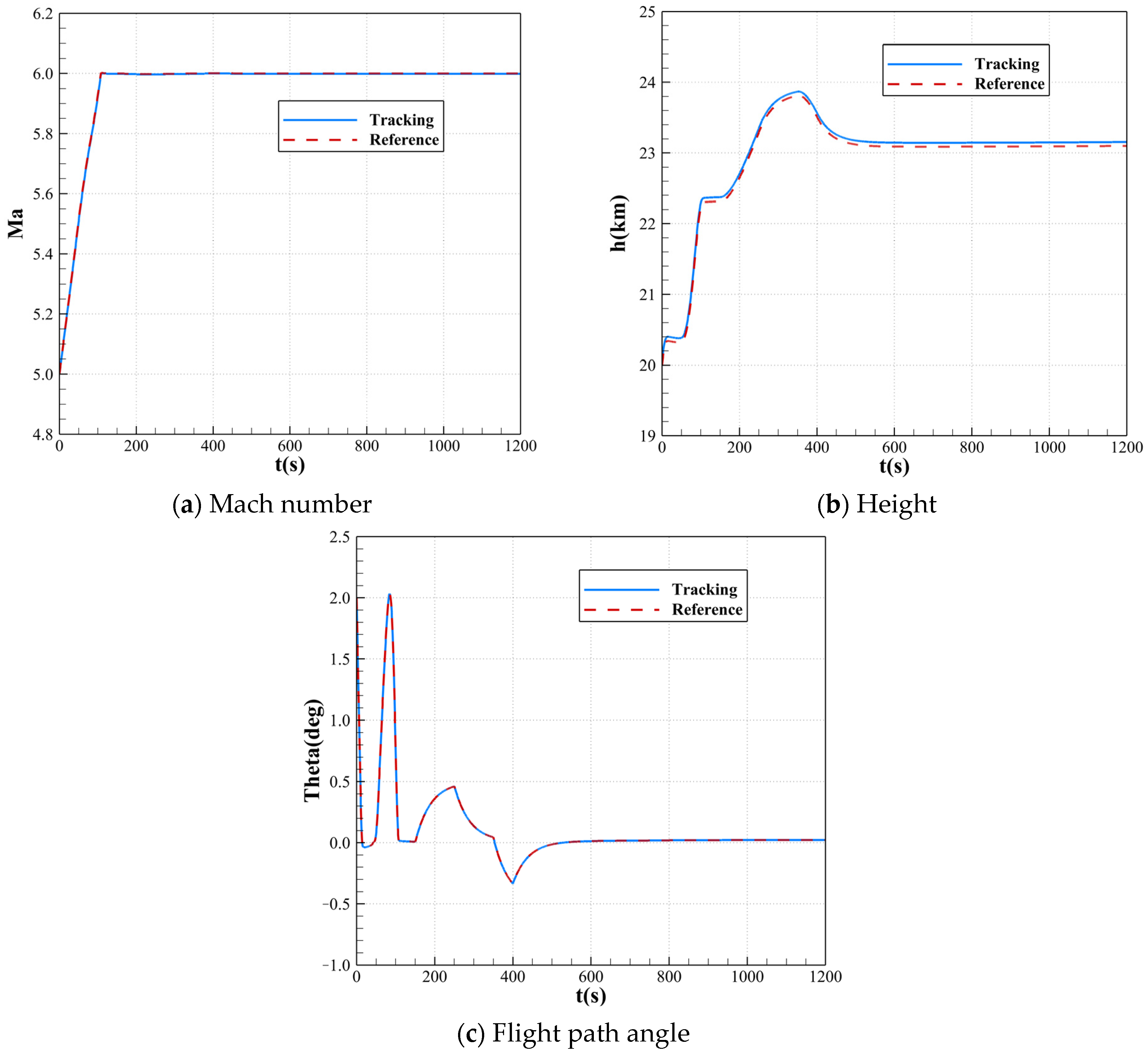
During longitudinal tracking, the Mach number, height, and flight path angle are selected as state variables. The tracking results under nominal conditions are shown in Figure 2. From Figure 2, it can be observed that the vehicle is able to track the reference trajectory effectively. The Mach number tracking curve in Figure 2a and the flight path angle tracking curve in Figure 2c align closely with the reference curves. However, there is a slight steady-state error in the height curve in Figure 2b, with the maximum error calculated to be 0.06 km.

Table 2. Tracking errors of state variables under nominal conditions.

Variable	MAE	RMSE	MRE (%)
Mach number	0.0012	0.0014	0.0208
Height (km)	0.0563	0.0566	0.2464
Flight path angle (deg)	9.6210 × 10−5	0.0003	0.3002

shows the tracking errors for each state variable under nominal conditions. As seen in the table, the errors for the Mach number and flight path angle are smaller than those for height, indicating better tracking performance for the former two. The maximum relative error for the Mach number is 0.4%, and for the flight path angle it is 0.2%, both of which are minimal.

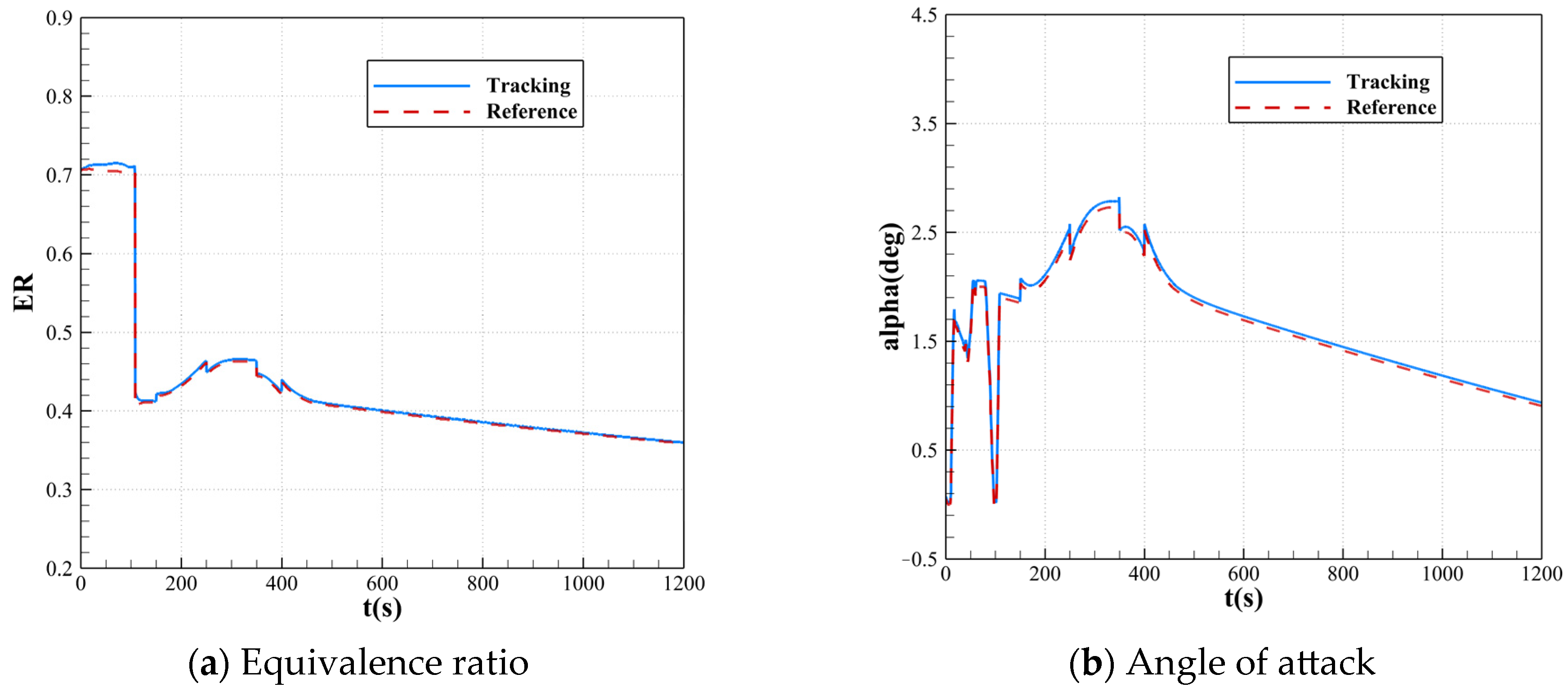
Figure 3 shows the control variable curves for trajectory tracking under nominal conditions. As seen in the figure, the equivalence ratio curve in Figure 3a and the angle of attack curve in Figure 3b closely follow the reference trajectories. During the acceleration stage from the starting point to Ma6, the actual equivalence ratio is slightly higher than the reference equivalence ratio. After reaching Ma6, the equivalence ratio curve aligns well with the reference, while the angle of attack curve shows minor overshoot, though this has little overall impact.

4.1.2. Deviation Simulation

From the results in Section 4.1.1, it is clear that under nominal conditions, the vehicle tracks the reference trajectory well, with very small tracking errors, demonstrating the designed controller performs well in tracking under nominal conditions. However, the characteristics of the vehicle, such as nonlinearity, strong coupling, and fast time-varying dynamics, along with uncertainties and disturbances during flight, like parameter variations, actuator errors, and noise, may affect flight stability. To verify the disturbance rejection capability of the controller, the axial force coefficient is subjected to extreme positive and negative deviations, with a deviation amplitude of 20%, while keeping the controller parameters unchanged. The simulation results are as follows.

Figure 4 shows the state variable curves for trajectory tracking under ±20% deviations in the axial force coefficient. From Figure 4a, it is observed that during the acceleration stage, the actual Mach number falls below the reference value under positive deviation, taking longer to reach the cruise Mach number. Conversely, under negative deviation, the actual Mach number matches the reference, suggesting that the controller handles negative deviations better than positive ones in terms of Mach number. In Figure 4c, under both positive and negative deviations, the flight path angle curves closely follow the reference, demonstrating that the controller effectively handles the impact of changes in the axial force coefficient on the flight path angle. For the height curves in Figure 4b, noticeable errors occur under both deviations. For further analysis, tracking errors for the state variables under axial force coefficient deviations are calculated and shown in

Table 3. Tracking errors of state variables under positive axial force coefficient deviation conditions.

Variable	MAE	RMSE	MRE (%)
Mach number	0.0186	0.0400	0.3178
Height (km)	0.0872	0.0906	0.3791
Flight path angle (deg)	0.0035	0.0067	12.9583

and

Table 4. Tracking errors of state variables under negative axial force coefficient deviation conditions.

Variable	MAE	RMSE	MRE (%)
Mach number	0.0015	0.0016	0.0254
Height (km)	0.0775	0.0781	0.3380
Flight path angle (deg)	0.0008	0.0009	3.6452

. The results reveal that height has the largest absolute error under both deviations, followed by Mach number, with the flight path angle having the smallest error. Additionally, errors under positive deviation are greater than those under negative deviation, indicating that the controller performs better under negative deviation than positive deviation.

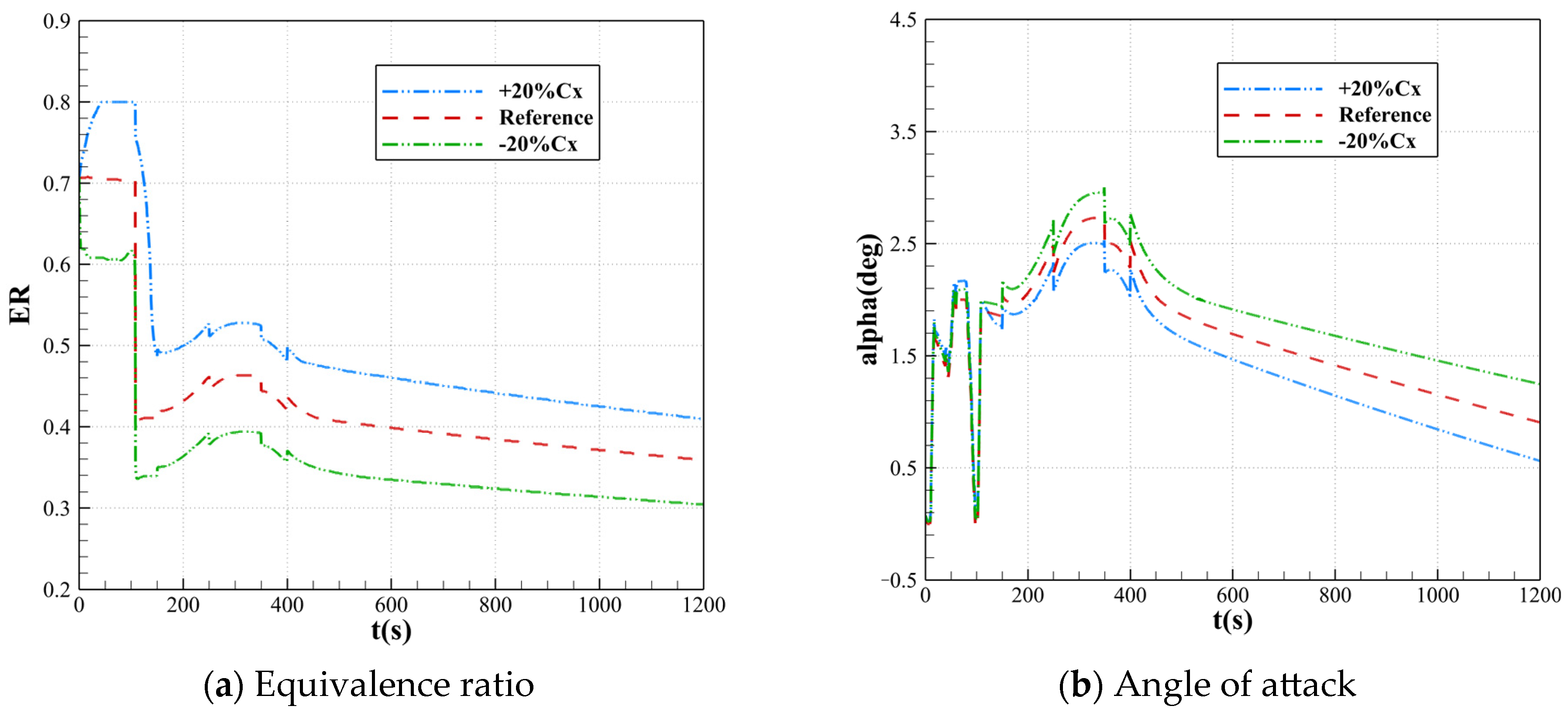
When the motion parameters of the vehicle change, its actual flight state will also change accordingly. Therefore, when the axial force coefficient is subjected to deviations, the expected flight Mach number and height are perturbed and altered. To maintain the intended reference trajectory, the control inputs must be adjusted, causing the control variable curves to differ from the original reference values, as illustrated in Figure 5.

4.2. Verification of Lateral Simulation

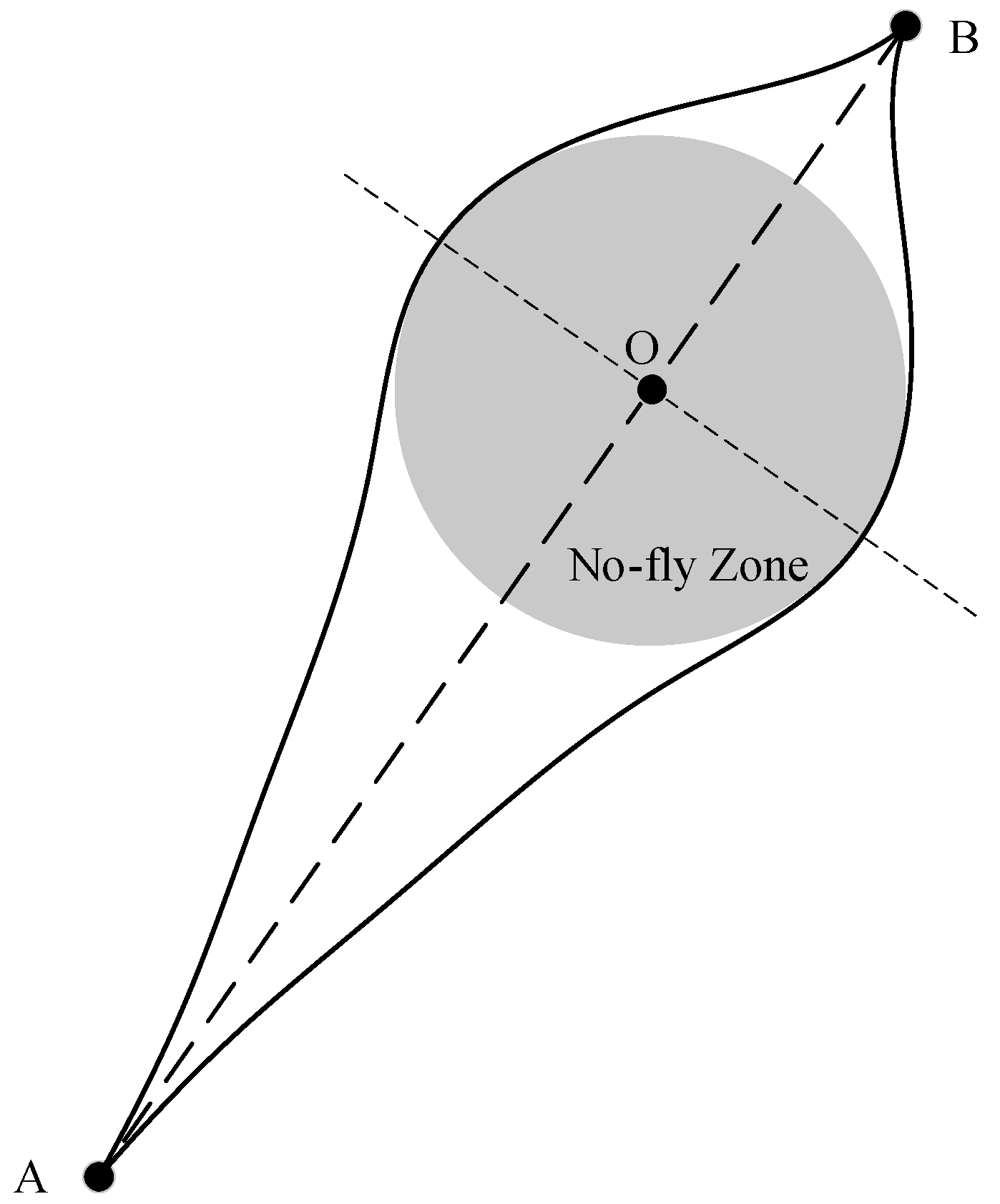
During actual flight, due to factors such as complex environments, geopolitical considerations, and electromagnetic interference, the vehicle may need to avoid no-fly zones. It is assumed that when the vehicle accelerates into the cruise stage, traveling from point $A$ to point $B$, there is a no-fly zone that must be circumvented. A schematic diagram of this scenario is shown in Figure 6.

By designing waypoint constraints and employing Bank-To-Turn (BTT) control, large-scale lateral maneuvers under no-fly zone constraints are achieved, obtaining a reference trajectory for lateral motion. This enables subsequent lateral trajectory tracking. The waypoint constraints are detailed in

Table 5. Waypoint constraints.

Waypoint	Latitude and Longitude
waypoint 1	(98.56°, 41.15°)
waypoint 2	(93.49°, 39.25°)
waypoint 3	(92.47°, 39.02°)
waypoint 4	(90.38°, 39.77°)
waypoint 5	(88.77°, 40.77°)

.

During lateral maneuvers, the controller aims to ensure that key parameters such as flight Mach number, height, flight path angle, lateral displacement, and track yaw angle precisely follow their desired reference values while avoiding no-fly zones.

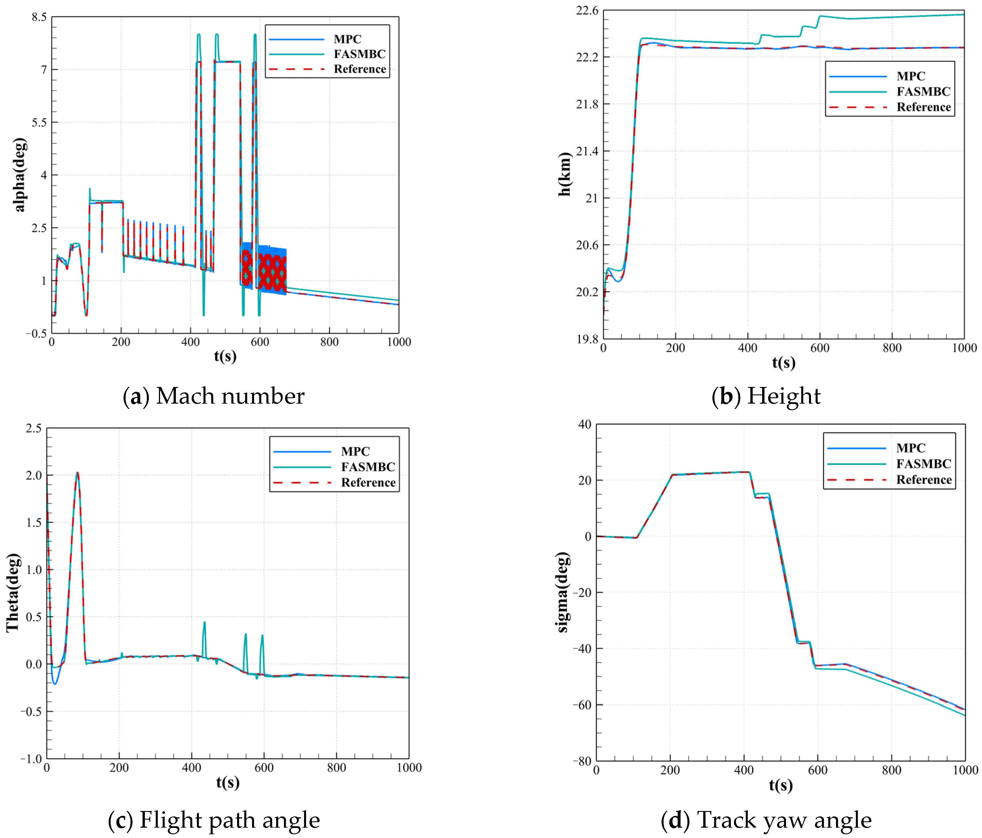
The simulation results are shown in Figure 7, where the blue solid line represents the trajectory tracking results using the model predictive controller designed in this paper under no-fly zone constraints. Specifically, Figure 7a–e display the state variable curves, while Figure 7f–h show the control variable curves.

Besides the three state variables—Mach number, height, and flight path angle, which are observed in the longitudinal plane simulation—lateral displacement and track yaw angle are also added during lateral maneuvers to evaluate tracking performance.

From the blue solid lines in Figure 7a–e, it can be observed that during the lateral maneuver to avoid the no-fly zones when using the model predictive control method, the flight trajectory aligns very well with the reference trajectory during the lateral maneuver to avoid the no-fly zone, with almost no error. This demonstrates that the designed controller performs effectively and has practical value in scenarios involving lateral maneuver tasks.

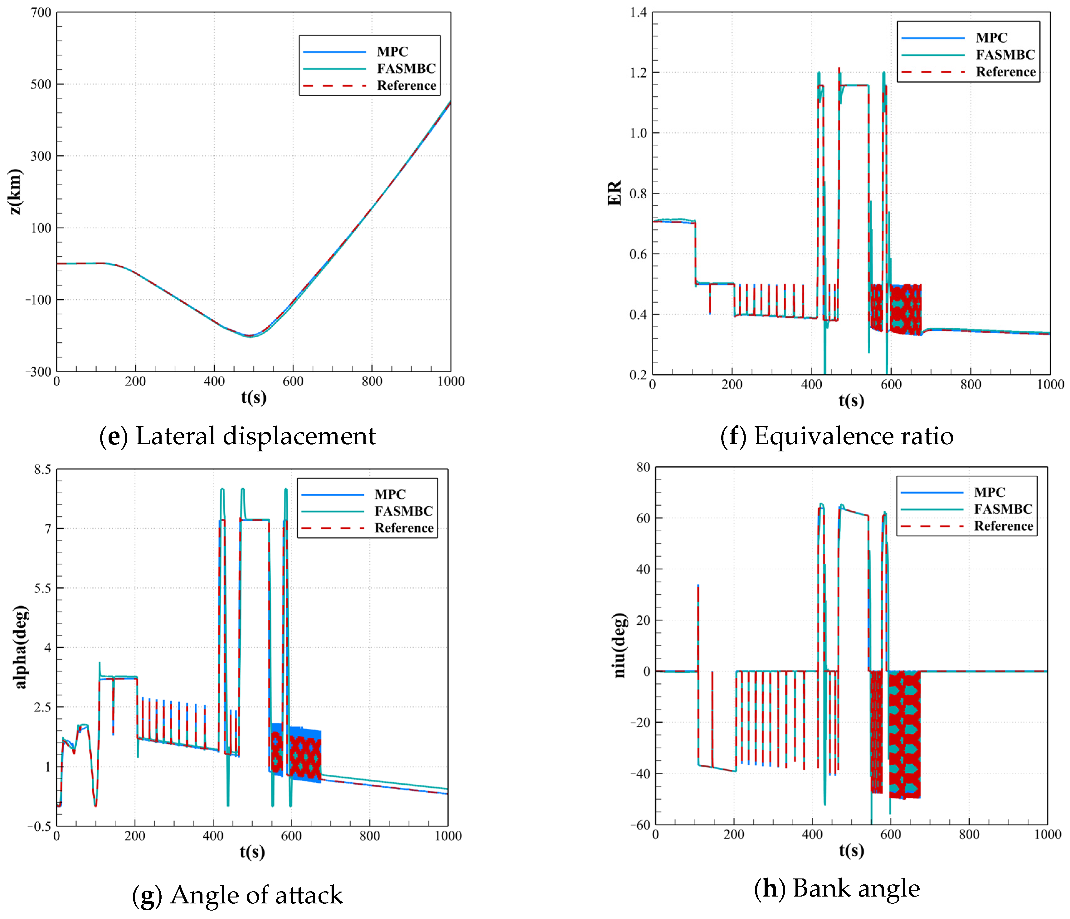
The control input curves for trajectory tracking under no-fly zone constraints are shown in Figure 7f–h. Besides the original equivalence ratio and angle of attack, the bank angle is added as a control input when using BTT for lateral maneuvers, with the bank angle in the range of [−90°, 90°]. It can be observed that during the actual flight when using the model predictive method, the variations in the control input curves align well with the reference trajectory. A slight overshoot in the angle of attack occurs between 525 s and 675 s, but it has little effect on the tracking performance. However, oscillations in the control inputs are observed during the flight, which result from the real-time calculation of the line-of-sight angle and track yaw angle during trajectory generation. For future research on the lateral maneuver issues discussed here, it is essential to address these oscillations, such as by introducing sliding filter functions, to prevent adverse effects on the stable operation and rapid response of the engine.

Furthermore, under same simulation conditions, we studied the tracking control problem under no-fly zone constraints using the finite-time adaptive sliding mode back-stepping controller (FASMBC) proposed in Ref. [36], with the corresponding results depicted by green solid lines in Figure 7. Comparative analysis reveals that the proposed model predictive control framework demonstrates superior tracking accuracy and flight stability in lateral maneuver trajectory tracking with no-fly zone constraints, particularly showing enhanced constraint-handling capabilities when addressing complex operational scenarios involving restricted airspace.

Table 6. Tracking errors of state variables under no-fly zone constraints based on MPC.

Variable	MAE	RMSE
Mach number	8.673 × 10−5	2.992 × 10−4
Height (km)	4.835 × 10−3	9.632 × 10−3
Flight path angle (deg)	8.833 × 10−3	2.406 × 10−2
Track yaw angle (deg)	0.123	0.175
Lateral displacement (km)	0.464	0.718

shows the mean absolute error and root mean square error of the state variables obtained by using model predictive control method for trajectory tracking under no-fly zone constraints.

Using the method proposed in Ref. [36], the calculated state tracking errors are summarized in

Table 7. Tracking errors of state variables under no-fly zone constraints based on FASMBC.

Variable	MAE	RMSE
Mach number	3.424 × 10−3	6.126 × 10−3
Height (km)	0.149	0.179
Flight path angle (deg)	0.011	0.052
Track yaw angle (deg)	1.003	1.298
Lateral displacement (km)	2.637	3.687

.

By comparing the above results, it can be found that when using MPC for lateral trajectory tracking under no-fly zone constraints, the errors of each state variable are smaller than those using sliding mode control method. It indicates that the MPC approach achieves higher tracking precision and demonstrates better adaptability in such scenarios.

5. Conclusions

This paper applies model predictive control to address the trajectory tracking control problem of hypersonic flight vehicles under complex constraints. Using MPC principles, the outputs are predicted, and the optimal control law is obtained through rolling optimization and feedback correction. This method reduces the reliance on precise models, simplifies controller design, and improves the robustness of the flight control system under parameter perturbations, as well as its adaptability to complex mission scenarios like no-fly zone avoidance. The simulation results show that the designed controller can effectively suppress the influence of aerodynamic parameter variations and maintain superior robustness. For instance, under nominal conditions, the average relative tracking errors are approximately 0.02% for Mach number and 0.25% for height. At under ±20% deviations in the axial force coefficient, the maximum average relative tracking errors for both Mach number and height remain below 0.4%. Furthermore, the proposed method for lateral maneuvering tracking control under no-fly zone constraints has more significant advantages and stronger adaptability, which enables precise trajectory tracking with no-fly zone constraints and provides a valuable reference for the maneuvering control of hypersonic flight vehicles.