Fast Entry Trajectory Planning Method for Wide-Speed Range UASs

Abstract

Convex optimization has gained increasing popularity in trajectory planning methods for wide-speed range unmanned aerial systems (UASs) with multiple no-fly zones (NFZs) in the entry phase. To address the issues of slow or even infeasible solutions, a modified fast trajectory planning method using the approaches of variable trust regions and adaptive generated initial values is proposed in this paper. A dimensionless energy-based dynamics model detailing the constraints of the entry phase is utilized to formulate the original entry trajectory planning problem. This problem is then transformed into a finite-dimensional convex programming problem, using techniques such as successive linearization and interval trapezoidal discretization. Finally, a variable trust region strategy and an adaptive initial value generation strategy are adopted to accelerate the solving process in complex flight environments. The experimental results imply that the strategy proposed in this paper can significantly reduce the solution time of trajectory planning for wide-speed range UASs in complex environments.

1. Introduction

Wide-speed range UASs possess the characteristics of an extensive speed region, large airspace, and extended endurance, which offer the advantages of flexible flight paths and strong maneuverability. The near-space entry phase necessitates a reference trajectory for the guidance systems to follow [1]; in addition, this optimized trajectory for the entry phase should take terminal constraints into consideration to alleviate load requirements in the terminal guidance phase [2]. These trajectories also need to meet a variety of in-flight constraints during the entry phase, with the aim of achieving mission objectives such as minimizing flight time and heat absorption. Consequently, the trajectory planning technology for UASs holds substantial research significance.

Diverse methods for tackling optimal control issues have been applied in solving trajectory planning problems, including pseudo-spectral methods, convex programming, and intelligent optimization techniques. Williams [3] addressed trajectory planning challenges by employing pseudo-spectral methods based on Legendre–Gauss–Lobatto (LGL) collocation techniques. Darby [4] improved the global pseudo-spectral method with an hp-adaptive method in terms of computational efficiency and solution precision. This method stood out for its ability to dynamically adjust the degrees of interpolating polynomials and the density of grid points, thereby balancing accuracy and efficiency. The authors of References [5,6,7] made significant progress in improving the pseudo-spectral method, tackling a broad spectrum of vehicle trajectory planning challenges. Despite the pseudo-spectral method having demonstrated some effectiveness in solving such problems, the issues of long computational time and the inability to guarantee optimality due to its direct method framework remain.

In contrast, convex programming, which operates within a convex set, ensures that the solutions obtained are globally optimal for the given problem. Therefore, it has been effectively applied in many aerospace applications, including spacecraft rendezvous and docking [8,9], formation flying [10,11], vehicle landing [12,13,14], and atmospheric flight [15,16]. Reference [17] presented a multi-stage convex programming approach designed for the rapid generation of re-entry trajectories that satisfied the specific path, waypoints, and NFZ constraints of conventional aviation vehicles (CAVs). Reference [18] utilized a sequential convex programming-based method for the cooperative re-entry trajectory planning of Hypersonic flight vehicles (HFVs) to address cooperative flight challenges. Marco [19] introduced an innovative drag-energy guidance scheme for atmospheric entry, based on pseudo-spectral and convex programming methods. The methods mentioned above did not take the complex flight environments seen with various NFZs into consideration; in the meantime, the solution’s efficiency is heavily reliant on the initial value selection, so it is necessary to develop a method to retain the global optimality of convex programming and accelerate its convergence when considering large-scale problems.

Therefore, this paper proposes an online rapid trajectory planning methodology that combines a variable trust region strategy coupled with an adaptive initial value generation strategy. The contributions of this research can be described as follows:

(1)

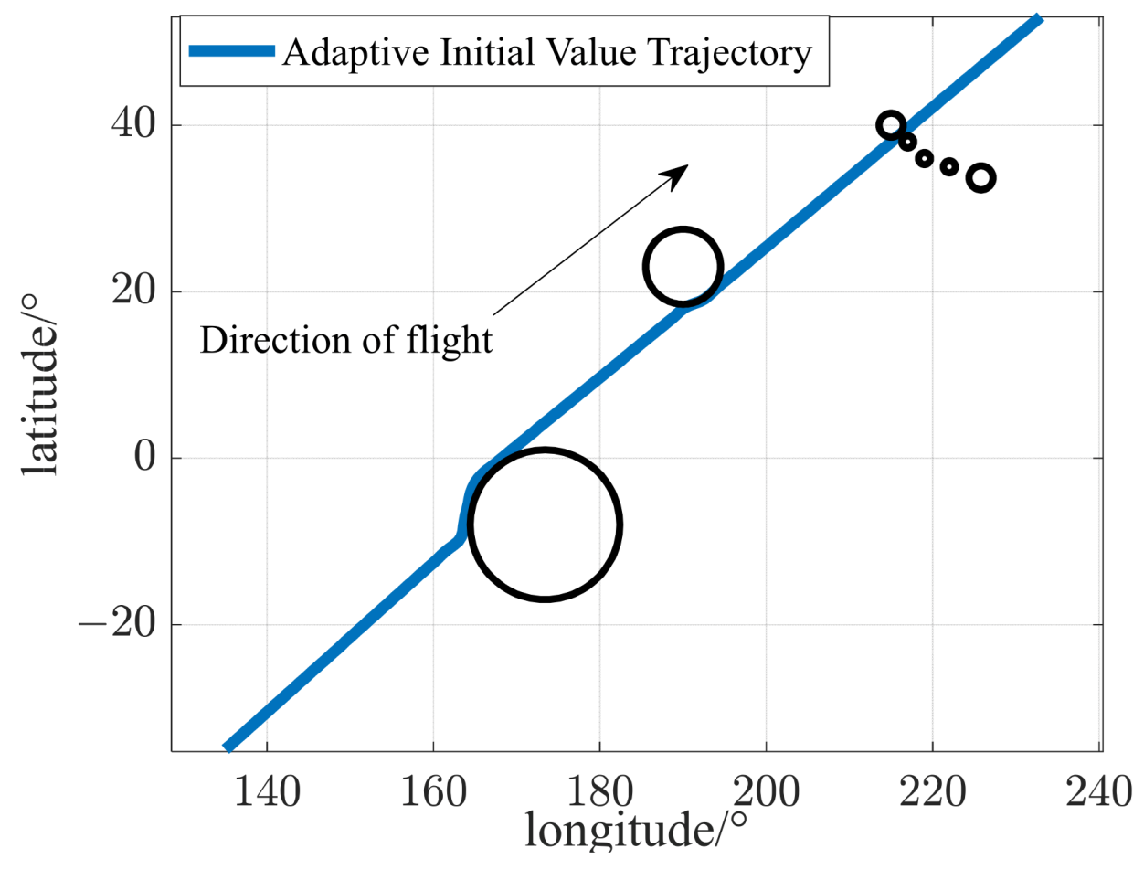
In terms of environmental adaptability, in order to solve the problem of the sensitivity of the initial value of convex programming in complex environments, this paper improves the traditional linear initial value generation method and proposes an adaptive initial value generation strategy to improve its solution ability.

(2)

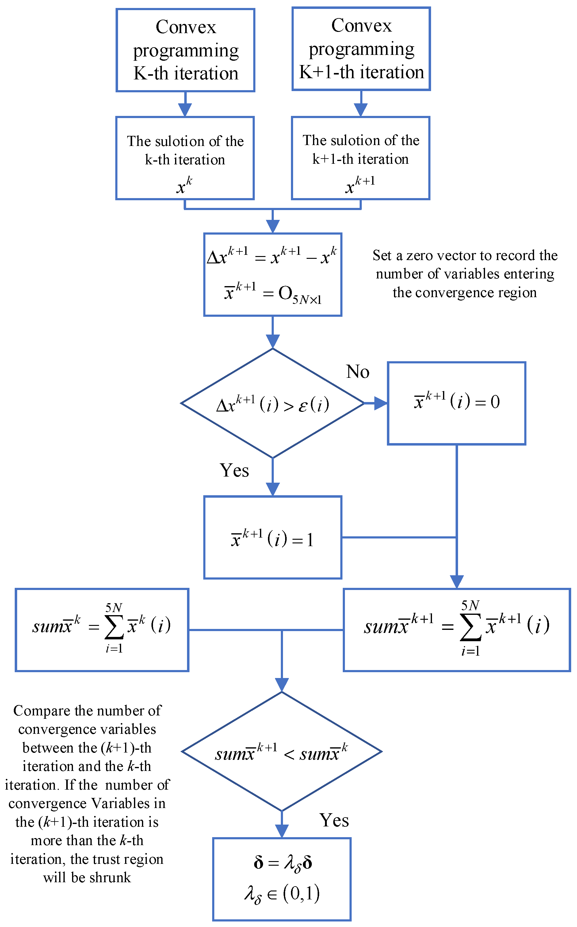
In terms of the convergence of the algorithm, which is different from the fixed trust region strategy of traditional algorithms, this paper proposes a variable trust region strategy that significantly improves the convergence speed of the algorithm and meets the needs of online applications.

The second section starts with an in-depth analysis of the UAS dynamic model and, based on this, the optimal control problem is established. The third section employs convex and interval-based trapezoidal discretization techniques to convert the original problem into a sequential convex programming problem. In the fourth section, a variable trust region strategy and an adaptive initial value generation strategy are proposed for complex environments. The superiority of the proposed method is verified by a comparative simulation in the fifth section, and the sixth section is a summary.

2. Formulation of the Entry Trajectory Planning Problem

2.1. UAS Motion Model

Considering the rotation of the Earth, the motion model of a UAS in the flightpath coordinate system can be established as follows:

$$\left\{\begin{array}{l}{\displaystyle \frac{dr}{dt}}=V\sin \gamma \\ {\displaystyle \frac{d\phi }{dt}}={\displaystyle \frac{V\cos \gamma \sin \psi }{r\cos \varphi }}\\ {\displaystyle \frac{d\varphi }{dt}}={\displaystyle \frac{V\cos \gamma \cos \psi }{r}}\\ {\displaystyle \frac{dV}{dt}}=-D-{\displaystyle \frac{\mu }{r^2}}\sin \gamma -{\Omega }_v\\ {\displaystyle \frac{d\gamma }{dt}}={\displaystyle \frac{L\cos \sigma }{V}}-{\displaystyle \frac{\mu \cos \gamma }{r^{2}V}}+{\displaystyle \frac{V\cos \gamma }{r}}+{\Omega }_{\gamma }\\ {\displaystyle \frac{d\psi }{dt}}={\displaystyle \frac{L\sin \sigma }{V\cos \gamma }}+{\displaystyle \frac{V\tan \varphi \cos \gamma \sin \psi }{r}}+{\Omega }_{\psi }\end{array}\right.$$

(1)

where $\mu$ is Earth’s gravitational constant; $m$ indicates the mass of the UAS; $r$, $V$ are the geocentric distance and the velocity of the UAS, respectively; $\phi$, $\varphi$ are the longitude and the latitude, respectively; $\gamma$, $\psi$, $\sigma$ are the flight path angle, the flight heading angle, and the flight bank angle, respectively. $L$ and $D$ are the lift acceleration and drag acceleration, defined as follows:

$$\begin{array}{l}L={\displaystyle \frac{C_L\rho V^{2}S}{2m}}\\ D={\displaystyle \frac{C_D\rho V^{2}S}{2m}}\end{array}$$

where $\rho ={\rho }_0\exp \left(-\left(r-R_0\right)/h_0\right)$ is the atmospheric density, $h_0$ and ${\rho }_0$ indicate the scale height and the atmospheric density at sea level; $S$ indicates the UAS’s reference area. $C_L$ and $C_D$ indicate the lift and drag coefficients, respectively, which are the function of the angle of attack and the velocity [20]:

$$\begin{array}{l}{C}_L=2.9451\alpha +0.2949{\mathrm{e}}^{-3.3943\times {10}^{-4}V}-0.2355\\ C_D=2.3795{\alpha }^2+0.3983{\mathrm{e}}^{-1.0794\times {10}^{-3}V}+0.0234\end{array}$$

(2)

Moreover, ${\Omega }_v$, ${\Omega }_{\gamma }$, and ${\Omega }_{\psi }$ represent terms related to the rotation of Earth, respectively, as follows:

$$\left\{\begin{array}{c}{\Omega }_v={\Omega }^{2}r\left(\cos \varphi \sin \varphi \cos \psi \cos \gamma -{\cos }^2\varphi \sin \gamma \right)\\ {\Omega }_{\gamma }={\displaystyle \frac{{\Omega }^{2}r\left(\cos \varphi \sin \varphi \cos \psi \sin \gamma +{\cos }^2\varphi \cos \gamma \right)}{V}}+2\Omega \sin \psi \cos \varphi \\ {\Omega }_{\psi }={\displaystyle \frac{{\Omega }^{2}r\cos \varphi \sin \varphi \sin \psi }{V\cos \gamma }}-{\displaystyle \frac{2\Omega \left(\cos \psi \sin \gamma \cos \varphi -\cos \gamma \sin \varphi \right)}{\cos \gamma }}\end{array}\right.$$

(3)

where $\Omega$ is the angular velocity of the Earth’s rotation.

During the actual entry flight phase of the UAS, the device is typically expected to reach a desired terminal condition with a specified terminal height and velocity. As the exact flight time cannot be predetermined, the approach taken in this paper is to use the dimensionless $\overline{e}$ as the independent variable to solve the problem effectively. Additionally, the variables in the system of equations are also dimensionless, to reduce the complexity of subsequent solutions. The resulting motion equations are as follows:

$$\left\{\begin{array}{l}{\displaystyle \frac{d\overline{r}}{d\overline{e}}}={\displaystyle \frac{d\overline{r}}{dt}}\cdot {\displaystyle \frac{dt}{d\overline{e}}}={\displaystyle \frac{\sin \gamma }{\overline{D}}}\\ {\displaystyle \frac{d\phi }{d\overline{e}}}={\displaystyle \frac{d\phi }{dt}}\cdot {\displaystyle \frac{dt}{d\overline{e}}}={\displaystyle \frac{\cos \gamma \sin \psi }{\overline{r}\overline{D}\cos \varphi }}\\ {\displaystyle \frac{d\varphi }{d\overline{e}}}={\displaystyle \frac{d\varphi }{dt}}\cdot {\displaystyle \frac{dt}{d\overline{e}}}={\displaystyle \frac{\cos \gamma \cos \psi }{\overline{r}\overline{D}}}\\ {\displaystyle \frac{d\gamma }{d\overline{e}}}={\displaystyle \frac{d\gamma }{dt}}\cdot {\displaystyle \frac{dt}{d\overline{e}}}={\displaystyle \frac{1}{{\overline{V}}^2\overline{D}}}\left(\overline{L}\cos \sigma +\left({\overline{V}}^2-{\displaystyle \frac{1}{\overline{r}}}\right){\displaystyle \frac{\cos \gamma }{\overline{r}}}+\overline{V}{\overline{\Omega }}_{\gamma }\right)\\ {\displaystyle \frac{d\psi }{d\overline{e}}}={\displaystyle \frac{d\psi }{dt}}\cdot {\displaystyle \frac{dt}{d\overline{e}}}={\displaystyle \frac{1}{{\overline{V}}^2\overline{D}}}\left({\displaystyle \frac{\overline{L}\sin \sigma }{\cos \gamma }}+{\displaystyle \frac{{\overline{V}}^2\cos \gamma \sin \psi \tan \varphi }{\overline{r}}}+\overline{V}{\overline{\Omega }}_{\psi }\right)\end{array}\right.$$

(4)

where $dt/d\overline{e}=R_0{g}_0/\left(\overline{V}\overline{D}+\overline{V}{\Omega }^2\overline{r}\left(\cos \varphi \sin \varphi \cos \psi \cos \gamma -{\cos }^2\varphi \sin \gamma \right)\right)$.

Since ${\Omega }^2\approx 5.3175\times {10}^{-9}$ is usually a small value, the above equation can be simplified as follows:

$$dt/d\overline{e}\approx R_0{g}_0/\overline{V}\overline{D}$$

(5)

In Equation (4), the variables are dimensionless variables, except for angles, and the specific treatments are as follows:

$$\left\{\begin{array}{l}\overline{r}={\displaystyle \frac{r}{R_0}}\\ \overline{V}={\displaystyle \frac{V}{\sqrt{g_0{R}_0}}}\\ \overline{t}={\displaystyle \frac{t}{\sqrt{R_0/g_0}}}\\ \overline{\Omega }={\displaystyle \frac{\Omega }{\sqrt{g_0/R_0}}}\\ \overline{e}={\displaystyle \frac{e}{\sqrt{g_0{R}_0}}}\\ \overline{L}={\displaystyle \frac{L}{g_0}}\\ \overline{D}={\displaystyle \frac{D}{g_0}}\end{array}\right.$$

(6)

The dimensionless energy in Equation (6) is expressed as:

$$\overline{e}={\displaystyle \frac{e}{\sqrt{g_0{R}_0}}}={\displaystyle \frac{\mu }{g_0{R}_{0}r}}-{\displaystyle \frac{{\overline{V}}^2}{2g_0{R}_0}}={\displaystyle \frac{1}{\overline{r}}}-{\displaystyle \frac{{\left(\overline{V}\right)}^2}{2}}$$

(7)

The dimensionless velocity can be derived from Equation (7):

$$\overline{V}=\sqrt{2\left({\displaystyle \frac{1}{\overline{r}}}-\overline{e}\right)}\approx \sqrt{2\left(1-\overline{e}\right)}$$

(8)

According to Equation (4), the state variables are selected as $x={\left[\overline{r},\phi ,\varphi ,\gamma ,\psi \right]}^T$. In the entry phase, the angle of the attack profile can usually be designed according to the velocity, and only the flight bank angle can be chosen as the control variable, that is, $u=\sigma$. When the optimal control variable is calculated, a robust flight controller is usually required for precise trajectory tracking, which has been proposed in [21,22]; therefore, the authors of this paper assumed that the tracking performance was ideal, and we carried out the subsequent research on this basis.

2.2. Constraints

Ensuring the UAS’s safety in the entry phase necessitates the consideration of multiple constraints, such as entry path constraints, control constraints, intrinsic constraints that are embedded within the motion equations, and initial and final condition constraints, as follows:

(1)

Equation of motion constraints

The equation of motion of the UAS, as shown in Equation (4), can be expressed as:

$$\begin{array}{l}\dot{x}\left(\overline{e}\right)=f\left(x\left(\overline{e}\right),u\left(\overline{e}\right),\overline{e}\right)\\ x\in {\mathbb{R}}^5,u\in \mathbb{R},\overline{e}\in \left[{\overline{e}}_0,{\overline{e}}_f\right]\end{array}$$

(9)

(2)

Entry path constraints

Because the UAS needs to withstand huge dynamic pressure and heat when flying at high velocity, it is necessary to introduce constraints on the heating rate $Q$ and dynamic pressure $q$ of the UAS. At the same time, to ensure the structural safety of the UAS flight, it is also necessary to constrain the normal load [23]. In the meantime, to avoid the adverse long-period oscillation effect, we must take the constraint of drag acceleration $D$ into consideration. The common path constraints can be expressed as:

$$\left\{\begin{array}{l}\dot{Q}=k_Q\sqrt{\overline{\rho }}{\left(\sqrt{g_0{R}_0}\overline{V}\right)}^{3.15}\le {\dot{Q}}_{\max }\\ q=0.5\overline{\rho }{\left(\sqrt{g_0{R}_0}\overline{V}\right)}^2\le q_{\max }\\ n=\sqrt{{\overline{L}}^2+{\overline{D}}^2}\le n_{\max }\\ \overline{D}\ge D_{\min }\end{array}\right.$$

(10)

where $k_Q=9.4369\times {10}^{-5}$ is a constant parameter, which is related to the type of UAS.

(3)

Control constraints

The flight bank angle $\sigma$ is selected as the control variable, with constraints as follows:

$${\sigma }_{\min }\le \left|\sigma \right|\le {\sigma }_{\max }$$

(11)

(4)

Initial constraints

The initial constraints can be described as follows:

$$x\left({\overline{e}}_0\right)=x_0$$

(12)

(5)

Terminal constraints

The terminal constraints can be defined as follows:

$$\left\{\begin{array}{l}\overline{r}\left({\overline{e}}_f\right)={\overline{r}}_f,\phi \left({\overline{e}}_f\right)={\phi }_f,\varphi \left({\overline{e}}_f\right)={\varphi }_f\\ \gamma \left({\overline{e}}_f\right)={\gamma }_f,\psi \left({\overline{e}}_f\right)={\psi }_f\end{array}\right.$$

(13)

(6)

NFZ constraints

This paper considers two types of NFZ constraints; the first is the cylindrical NFZ, which can be characterized as follows:

$${\left(\phi -{\phi }_c\right)}^2+{\left(\varphi -{\varphi }_c\right)}^2\ge d^2$$

(14)

where ${\phi }_c$ and ${\varphi }_c$ are the longitude and latitude of the center of the circle projected on the ground by the NFZ; $d$ is the radius of the NFZ.

The second constraint is the spherical NFZ, which can be presented as follows:

$${\left(\phi -{\phi }_c\right)}^2+{\left(\varphi -{\varphi }_c\right)}^2+{\left(\overline{r}-{\overline{r}}_c\right)}^2\ge d^2$$

(15)

where $\overline{r}$ is the geocentric distance of the center of the NFZ.

2.3. Performance Index

To get a time-minimal trajectory of the UAS, the performance index is described as follows:

$$J={\displaystyle {\int }_{t_0}^{t_f}1}dt={\displaystyle {\int }_{{\overline{e}}_0}^{{\overline{e}}_f}\frac{1}{\overline{D}\overline{V}}d\overline{e}}$$

(16)

In summary, the mathematical description of the original optimal control problem P0 is as follows:

$$\begin{array}{l}\mathrm{P}0:\min J={\displaystyle {\int }_{{\overline{e}}_0}^{{\overline{e}}_f}\frac{1}{\overline{D}\overline{V}}d\overline{e}}\\ s.t.\left\{\begin{array}{l}\dot{x}\left(\overline{e}\right)=f\left(x\left(\overline{e}\right),u\left(\overline{e}\right),\overline{e}\right),\overline{e}\in \left[{\overline{e}}_0,{\overline{e}}_f\right]\\ \dot{Q}=k_Q\sqrt{\overline{\rho }}{\left(\sqrt{g_0{R}_0}\overline{V}\right)}^{3.15}\le {\dot{Q}}_{\max }\\ q=0.5\overline{\rho }{\left(\sqrt{g_0{R}_0}\overline{V}\right)}^2\le q_{\max }\\ n=\sqrt{{\overline{L}}^2+{\overline{D}}^2}\le n_{\max }\\ {\sigma }_{\min }\le \left|\sigma \right|\le {\sigma }_{\max }\\ x\left({\overline{e}}_0\right)=x_0\\ x\left({\overline{e}}_f\right)=x_f\end{array}\right.\end{array}$$

(17)

3. Convexification and Discretization of the Original Optimal Control Problem

In order to solve problem P0 using convex programming, it is necessary to transform P0 into a finite-dimensional convex programming problem. Therefore, this section employs methods such as sequential linearization to convexify problem P0 and applies trapezoidal discretization to establish a convex programming model, P2.

3.1. Convexification of Constraints

3.1.1. Equivalent Transformations of Entry Path Constraints

First, take the logarithm of both sides of Equation (10), and then use a finite number of linear transformations to convert the constraints into the following linear form:

$$\left\{\begin{array}{l}\overline{r}\left(\overline{e}\right)\ge l_Q\left(\overline{e}\right)=1+h_0\ln {\displaystyle \frac{k_Q^2{\rho }_0{g}_0^{3.15}{R}_0^{3.15}{\left(2-2\overline{e}\right)}^{3.15}}{{\dot{Q}}_{\max }^2}}\\ \overline{r}\left(\overline{e}\right)\ge l_q\left(\overline{e}\right)=1+h_0\ln {\displaystyle \frac{{\rho }_0{g}_0{R}_0\left(1-\overline{e}\right)}{q_{\max }}}\\ \overline{r}\left(\overline{e}\right)\ge l_n\left(\overline{e}\right)=1+h_0\ln {\displaystyle \frac{{\rho }_0{R}_0\left(1-\overline{e}\right)S\sqrt{{C_L}^2+{C_D}^2}}{n_{\max }m}}\\ \overline{r}\left(\overline{e}\right)\le {\overline{r}}_{\max }\left(\overline{e}\right)=1+h_0\ln {\displaystyle \frac{{\rho }_0{R}_0\left(1-\overline{e}\right)S{C}_D}{D_{\min }m}}\end{array}\right.$$

(18)

Equation (18) is equivalent to:

$$\left\{\begin{array}{l}\overline{r}\left(\overline{e}\right)\ge {\overline{l}}_{\min }\left(\overline{e}\right)=\max \left\{l_Q\left(\overline{e}\right),l_q\left(\overline{e}\right),l_n\left(\overline{e}\right)\right\}\\ \overline{r}\left(\overline{e}\right)\le {\overline{r}}_{\max }\left(\overline{e}\right)\end{array}\right.$$

(19)

3.1.2. Slack Method for Control Constraints

When the control variable is selected as $\sigma$, the linearization of the differential equation can lead to oscillations in the solution due to the coupling between the control variable and the state variables. To alleviate this phenomenon, the control variable is reformulated as follows:

$$u\triangleq {\left[u_1,u_2\right]}^T={\left[\cos \sigma ,\sin \sigma \right]}^T$$

(20)

Then, the control constraints can be replaced with:

$$\begin{array}{c}\cos {\sigma }_{\max }\le u_1\le \cos {\sigma }_{\min }\\ u_1^2+u_2^2=1\end{array}$$

(21)

where the equation is still non-convex, and the constraints are handled using the slack method, which is expressed as:

$$u_1^2+u_2^2\le 1$$

(22)

Therefore, the control constraints are expanded into a convex set, with the regularization terms designed in the following section to guarantee that the optimal solution after slacking the constraints will remain on the convex set boundaries.

3.1.3. Linearization of the Performance Index

Equation (16) can be described as follows:

$$J={\displaystyle {\int }_{{\overline{e}}_0}^{{\overline{e}}_f}\frac{1}{\overline{D}\overline{V}}d\overline{e}}={\displaystyle \frac{2m}{R_{0}S{C}_D{\overline{V}}^3}}{\displaystyle {\int }_{{\overline{e}}_0}^{{\overline{e}}_f}\frac{1}{\overline{\rho }}d\overline{e}}\triangleq a_0{\displaystyle {\int }_{{\overline{e}}_0}^{{\overline{e}}_f}\frac{1}{\overline{\rho }}d\overline{e}}$$

(23)

Since $\overline{V}$ can be explained as a function of $\overline{e}$ as in Equation (8), only $\overline{\rho }$ in Equation (23) is related to the optimization variable. If we linearize Equation (23) and let $a_0=2m/\left(R_{0}S{C}_D{\overline{V}}^3\right)$, then we have:

$$\begin{array}{ll}{\displaystyle \frac{a_0}{\overline{\rho }}}& \approx a_0{\left.{\displaystyle \frac{d\left(1/\overline{\rho }\right)}{d\overline{r}}}\right|}_{\overline{r}={\overline{r}}^{\left(k\right)}}\cdot \left(\overline{r}-{\overline{r}}^{\left(k\right)}\right)+a_0{\left.{\displaystyle \frac{1}{\overline{\rho }}}\right|}_{\overline{r}={\overline{r}}^{\left(k\right)}}\\ & ={\left.-{\displaystyle \frac{a_0}{{\overline{\rho }}^2}}{\displaystyle \frac{d\overline{\rho }}{d\overline{r}}}\right|}_{\overline{r}={\overline{r}}^{\left(k\right)}}\cdot \left(\overline{r}-{\overline{r}}^{\left(k\right)}\right)+a_0{\left.{\displaystyle \frac{1}{\overline{\rho }}}\right|}_{\overline{r}={\overline{r}}^{\left(k\right)}}\\ & =-a_0{\displaystyle \frac{{\overline{\rho }}_{\overline{r}}^{\left(k\right)}}{{\left({\overline{\rho }}^{\left(k\right)}\right)}^2}}\overline{r}+a_0\left({\displaystyle \frac{{\overline{\rho }}_{\overline{r}}^{\left(k\right)}}{{\left({\overline{\rho }}^{\left(k\right)}\right)}^2}}{\overline{r}}^{\left(k\right)}+{\displaystyle \frac{1}{{\overline{\rho }}^{\left(k\right)}}}\right)\\ & \triangleq c_1^{\left(k\right)}\left(\overline{V},\overline{e}\right)\overline{r}+c_0^{\left(k\right)}\left(\overline{V},\overline{e}\right)\end{array}$$

(24)

where ${\overline{\rho }}^{\left(k\right)}$ is the density of the atmosphere corresponding to the geocentric distance of ${\overline{r}}^{\left(k\right)}\left(e\right)$ at the $k$-th iteration; ${\overline{\rho }}_{\overline{r}}^{\left(k\right)}$ is the derivative of $\overline{\rho }$ to $\overline{r}$ at ${\overline{r}}^{\left(k\right)}\left(\overline{e}\right)$.

To guarantee that the slacked constraints can achieve solutions on their boundaries, a regularization term is incorporated into the performance index. This regularization term constrains the slacked control variables to take values on their boundaries. The revised performance index is shown in Equation (25).

$$J={\displaystyle {\int }_{{\overline{e}}_0}^{{\overline{e}}_f}\left(c_1\left(\overline{V},\overline{e}\right)\overline{r}+c_0\left(\overline{V},\overline{e}\right)+{\epsilon }_{\psi }\psi \right)d\overline{e}}$$

(25)

3.1.4. Convexification of Terminal Constraints

Due to the original forms of the terminal constraints being linear equality constraints, no convexification is required. However, within the framework of convex programming, the constraints on terminal latitude and longitude are overly strict, which may lead to situations where they cannot be satisfied during the initial optimization process. To reduce the risk of infeasibility, two penalty terms, denoted as $\Delta \phi$ and $\Delta \varphi$, are incorporated into the performance index. These items ensure that even if the algorithm fails to achieve the predetermined target position during the iteration process, the terminal position will be driven towards the desired value. The penalty function is formulated as follows:

$$d\left(\phi \left({\overline{e}}_f\right),\varphi \left({\overline{e}}_f\right)\right)=c_{\phi }\left|\Delta \phi \right|+c_{\varphi }\left|\Delta \varphi \right|$$

(26)

where $c_{\phi }>0$, $c_{\varphi }>0$ are coefficients: $\Delta \phi =\phi \left(e_f\right)-{\phi }_f$, $\Delta \varphi =\varphi \left(e_f\right)-{\varphi }_f$.

Since Equation (26) is nonconvex, two variables $\vartheta$ and $\Phi$ are proposed to slack it, as shown in Equation (27):

$$\min \overline{d}\left(\vartheta ,\Phi \right)=c_{\phi }\vartheta +c_{\varphi }\Phi$$

(27)

These two slack variables also satisfy the inequality constraints:

$$\left|\phi \left({\overline{e}}_f\right)-{\phi }_f\right|\le \vartheta ,\left|\varphi \left({\overline{e}}_f\right)-{\varphi }_f\right|\le \Phi$$

(28)

At this point, the full performance index can be expressed as follows:

$$J=c_{\phi }\vartheta +c_{\varphi }\Phi +{\displaystyle {\int }_{{\overline{e}}_0}^{{\overline{e}}_f}\left(c_1\left(\overline{V},\overline{e}\right)\overline{r}+c_0\left(\overline{V},\overline{e}\right)+{\epsilon }_{\psi }\psi \right)d\overline{e}}$$

(29)

By adjusting the values of parameters $c_{\phi }$, $c_{\varphi }$, and ${\epsilon }_{\psi }$, the penalty terms in the performance index can be infinitely close to 0, and there is also strict proof [24] for the introduced regularization term so that the control constraints can be taken to their boundaries.

3.1.5. Linearization of the Equation of Motion

After the control variables are converted, Equation (4) can be expressed as:

$$x^{\prime }=f\left(x,u,\overline{e}\right)=f_1\left(x,\overline{e}\right)+B\left(x,\overline{e}\right)u$$

(30)

Near the solution of the k-th iteration, we linearize Equation (30) as:

$$\begin{array}{l}{x}^{\prime }=A\left(x^{\left(k\right)}\right)x+B\left(x^{\left(k\right)}\right)u+b\left(x^{\left(k\right)}\right)\\ \left\{\begin{array}{l}A\left(x^{\left(k\right)}\right)={\displaystyle \frac{\partial f_0\left(x^{\left(k\right)}\right)}{\partial x^T}}\\ =\left[\begin{array}{ccccc}-{\displaystyle \frac{{\overline{D}}_{\overline{r}}^{\left(k\right)}\sin {\gamma }^{\left(k\right)}}{{\left({\overline{D}}^{\left(k\right)}\right)}^2}}& 0& 0& {\displaystyle \frac{\cos {\gamma }^{\left(k\right)}}{{\overline{D}}^{\left(k\right)}}}& 0\\ a_{21}& 0& {\displaystyle \frac{\cos {\gamma }^{\left(k\right)}\sin {\psi }^{\left(k\right)}\sin {\varphi }^{\left(k\right)}}{r^{\left(k\right)}{\overline{D}}^{\left(k\right)}{\cos }^2{\varphi }^{\left(k\right)}}}& -{\displaystyle \frac{\sin {\gamma }^{\left(k\right)}\sin {\psi }^{\left(k\right)}}{{\overline{r}}^{\left(k\right)}{\overline{D}}^{\left(k\right)}\cos {\varphi }^{\left(k\right)}}}& {\displaystyle \frac{\cos {\gamma }^{\left(k\right)}\cos {\psi }^{\left(k\right)}}{{\overline{r}}^{\left(k\right)}{\overline{D}}^{\left(k\right)}\cos {\varphi }^{\left(k\right)}}}\\ a_{31}& 0& 0& -{\displaystyle \frac{\sin {\gamma }^{\left(k\right)}\cos {\psi }^{\left(k\right)}}{{\overline{r}}^{\left(k\right)}{\overline{D}}^{\left(k\right)}}}& -{\displaystyle \frac{\cos {\gamma }^{\left(k\right)}\sin {\psi }^{\left(k\right)}}{{\overline{r}}^{\left(k\right)}{\overline{D}}^{\left(k\right)}}}\\ a_{41}& 0& 0& {\displaystyle \frac{\sin {\gamma }^{\left(k\right)}}{{\overline{r}}^{\left(k\right)}{\overline{D}}^{\left(k\right)}}}\left({\displaystyle \frac{1}{{\overline{r}}^{\left(k\right)}{\left({\overline{V}}^{\left(k\right)}\right)}^2}}-1\right)& 0\\ a_{51}& 0& {\displaystyle \frac{\cos {\gamma }^{\left(k\right)}\sin {\psi }^{\left(k\right)}}{{\overline{r}}^{\left(k\right)}{\overline{D}}^{\left(k\right)}{\cos }^2{\varphi }^{\left(k\right)}}}& -{\displaystyle \frac{\sin {\gamma }^{\left(k\right)}\sin {\psi }^{\left(k\right)}\tan {\varphi }^{\left(k\right)}}{{\overline{r}}^{\left(k\right)}{\overline{D}}^{\left(k\right)}}}& {\displaystyle \frac{\cos {\gamma }^{\left(k\right)}\cos {\psi }^{\left(k\right)}\tan {\varphi }^{\left(k\right)}}{{\overline{r}}^{\left(k\right)}{\overline{D}}^{\left(k\right)}}}\end{array}\right]\\ b\left(x^{\left(k\right)}\right)=f_0\left(x^{\left(k\right)}\right)-A\left(x^{\left(k\right)}\right)x^{\left(k\right)}+f_{\Omega }\left(x^{\left(k\right)}\right)\end{array}\right.\end{array}$$

(31)

where:

$$\left\{\begin{array}{l}{\overline{D}}_{\overline{r}}^{\left(k\right)}=\partial \overline{D}\left(x^{\left(k\right)}\right)/\partial \overline{r}=-{\displaystyle \frac{R_{0}S{\rho }_0{\left({\overline{V}}^{\left(k\right)}\right)}^2{C}_D^{\left(k\right)}{e}^{\left(\left(1-{\overline{r}}^{\left(k\right)}\right)/h_0\right)}}{2m{h}_0}}\\ a_{21}=-\left({\displaystyle \frac{{\overline{D}}_{\overline{r}}^{\left(k\right)}}{{\overline{r}}^{\left(k\right)}{\left({\overline{D}}^{\left(k\right)}\right)}^2}}+{\displaystyle \frac{1}{{\left({\overline{r}}^{\left(k\right)}\right)}^2{\overline{D}}^{\left(k\right)}}}\right){\displaystyle \frac{\cos {\gamma }^{\left(k\right)}\sin {\psi }^{\left(k\right)}}{\cos {\varphi }^{\left(k\right)}}}\\ a_{31}=-\left({\displaystyle \frac{{\overline{D}}_r^{\left(k\right)}}{{\overline{r}}^{\left(k\right)}{\left({\overline{D}}^{\left(k\right)}\right)}^2}}+{\displaystyle \frac{1}{{\left({\overline{r}}^{\left(k\right)}\right)}^2{\overline{D}}^{\left(k\right)}}}\right)\cos {\gamma }^{\left(k\right)}\cos {\psi }^{\left(k\right)}\\ a_{41}={\displaystyle \frac{{\overline{D}}_r^{\left(k\right)}\cos {\gamma }^{\left(k\right)}}{{\overline{r}}^{\left(k\right)}{\left({\overline{D}}^{\left(k\right)}\right)}^2}}\left({\displaystyle \frac{1}{{\overline{r}}^{\left(k\right)}{\left({\overline{V}}^{\left(k\right)}\right)}^2}}-1\right)+{\displaystyle \frac{\cos {\gamma }^{\left(k\right)}}{{\overline{D}}^{\left(k\right)}{\left({\overline{r}}^{\left(k\right)}\right)}^2}}\left({\displaystyle \frac{2}{{\overline{r}}^{\left(k\right)}{\left({\overline{V}}^{\left(k\right)}\right)}^2}}-1\right)\\ a_{51}=-{\displaystyle \frac{D_r^{\left(k\right)}\cos {\gamma }^{\left(k\right)}\sin {\psi }^{\left(k\right)}\tan {\varphi }^{\left(k\right)}}{{\overline{r}}^{\left(k\right)}{\left({\overline{D}}^{\left(k\right)}\right)}^2}}-{\displaystyle \frac{\cos {\gamma }^{\left(k\right)}\sin {\psi }^{\left(k\right)}\tan {\varphi }^{\left(k\right)}}{{\left({\overline{r}}^{\left(k\right)}\right)}^2{\overline{D}}^{\left(k\right)}}}\\ f_{\Omega }={\left[0,0,0,{\displaystyle \frac{1}{{\left({\overline{V}}^{\left(k\right)}\right)}^2{\overline{D}}^{\left(k\right)}}}{\overline{\Omega }}_{\gamma }^{\left(k\right)},{\displaystyle \frac{1}{{\left({\overline{V}}^{\left(k\right)}\right)}^2{\overline{D}}^{\left(k\right)}}}{\overline{\Omega }}_{\psi }^{\left(k\right)}\right]}^T\end{array}\right..$$

In order to avoid large deviations in the process of successive linearization, a trust region constraint needs to be introduced, which is given in the following form:

$$\left|x^{\left(k+1\right)}-x^{\left(k\right)}\right|\le \delta$$

(32)

where $\delta \in {\mathbb{R}}^{5\times 1}$ is a constant vector.

3.1.6. Conversion of NFZ Constraints

Using the successive linearization method, the linearized expression of the cylindrical NFZ constraint in Equation (14) can be obtained:

$$2\left({\phi }^{(k)}-{\phi }_{ci}\right)\phi +2\left({\varphi }^{(k)}-{\varphi }_{ci}\right)\varphi \ge {d_{ci}}^2+{\overline{d}}_c$$

(33)

where ${\phi }^{(k)}$ and ${\varphi }^{(k)}$ are the results of the $k$-th iteration; ${\phi }_{ci}$, ${\varphi }_{ci}$, and $d_{ci}$ are the longitude, latitude, and radius of the center of the circle projected on the ground by the $i$-th cylindrical NFZ ($i=1,2\dots M_1$), and they satisfy the following:

$$\begin{array}{c}{\overline{d}}_c=-{\left({\phi }^{(k)}-{\phi }_{ci}\right)}^2-{\left({\varphi }^{(k)}-{\varphi }_{ci}\right)}^2+2\left({\phi }^{(k)}-{\phi }_{ci}\right){\phi }^{(k)}\\ +2\left({\varphi }^{(k)}-{\varphi }_{ci}\right){\varphi }^{(k)}\end{array}$$

(34)

The linearized expression for the spherical NFZ in Equation (15) is further derived as follows:

$$2\left[\left({\phi }^{(k)}-{\phi }_{bi}\right)\phi +\left({\varphi }^{(k)}-{\varphi }_{bi}\right)\varphi +\left({\overline{r}}^{(k)}-{\overline{r}}_{bi}\right)\overline{r}\right]\ge {d_{bi}}^2+{\overline{d}}_b$$

(35)

where ${\phi }^{(k)}$ and ${\varphi }^{(k)}$ are the values of longitude and latitude of the $k$-th iteration; ${\phi }_{ci}$, ${\varphi }_{ci}$, ${\overline{r}}^{(k)}$ and $d_{ci}$ are the longitude, latitude, geocentric distance, and radius of the center of the $i$-th spherical NFZ ($i=1,2\dots M_2$), respectively, and they satisfy the following:

$$\begin{array}{c}\overline{d}=-{\left({\phi }^{(k)}-{\phi }_{ci}\right)}^2-{\left({\varphi }^{(k)}-{\varphi }_{ci}\right)}^2-{\left({\overline{r}}^{(k)}-{\overline{r}}_{ci}\right)}^2\\ +2\left({\phi }^{(k)}-{\phi }_{ci}\right){\phi }^{(k)}+2\left({\varphi }^{(k)}-{\varphi }_{ci}\right){\varphi }^{(k)}+2\left({\overline{r}}^{(k)}-{\overline{r}}_{ci}\right){\overline{r}}^{(k)}\end{array}$$

(36)

Through the above processing calculations, the sequential convex optimal control problem P1 is obtained:

$$\begin{array}{c}\mathrm{P}1:\min c_{\phi }\vartheta +c_{\varphi }\Phi +{\displaystyle {\int }_{{\overline{e}}_0}^{{\overline{e}}_f}{c}_1\left(\overline{V},\overline{e}\right)\overline{r}+c_0\left(\overline{V},\overline{e}\right)+{\epsilon }_{\psi }\psi d\overline{e}}\\ \begin{array}{c}s.t.x^{\prime }=A\left(x^{\left(k\right)}\right)x+B\left(x^{\left(k\right)}\right)u+b\left(x^{\left(k\right)}\right)\\ x\left({\overline{e}}_0\right)=x_0\end{array}\\ \left|x^{\left(k+1\right)}\left(\overline{e}\right)-x^{\left(k\right)}\left(\overline{e}\right)\right|\le \delta \\ u_1^2\left(\overline{e}\right)+u_2^2\left(\overline{e}\right)\le 1\\ \cos {\sigma }_{\max }\le u_1\le \cos {\sigma }_{\min }\\ \begin{array}{l}\overline{r}\left(\overline{e}\right)\ge \overline{l}\left(\overline{e}\right)\\ \overline{r}\left(\overline{e}\right)\le {\overline{r}}_{\max }\left(\overline{e}\right)\end{array}\\ \left|\phi \left({\overline{e}}_f\right)-{\phi }_f\right|\le \vartheta ,\left|\varphi \left({\overline{e}}_f\right)-{\varphi }_f\right|\le \Phi \\ \overline{r}\left({\overline{e}}_f\right)={\overline{r}}_f,\gamma \left({\overline{e}}_f\right)={\gamma }_f,\psi \left({\overline{e}}_f\right)={\psi }_f\\ 2\left({\phi }^{(k)}-{\phi }_{ci}\right)\phi +2\left({\varphi }^{(k)}-{\varphi }_{ci}\right)\varphi \ge {d_{ci}}^2+{\overline{d}}_c\\ 2\left[\left({\phi }^{(k)}-{\phi }_{bi}\right)\phi +\left({\varphi }^{(k)}-{\varphi }_{bi}\right)\varphi +\left({\overline{r}}^{(k)}-{\overline{r}}_{bi}\right)\overline{r}\right]\ge {d_{bi}}^2+{\overline{d}}_b\end{array}$$

(37)

The sequential solution process will converge if:

$$\left|x^{\left(k+1\right)}\left(\overline{e}\right)-x^{\left(k\right)}\left(\overline{e}\right)\right|\le \epsilon ,\forall \overline{e}\in \left[{\overline{e}}_0,{\overline{e}}_f\right]$$

(38)

where $x^{\left(k+1\right)}\left(\overline{e}\right)$ and $\epsilon \in {\mathbb{R}}^5$ are the solution of the $\left(k+1\right)$-th iteration and a constant vector, respectively.

3.2. Discretization

To solve the sequential convex optimal control problem P1, this section uses an interval trapezoidal discretization method to convert the P1 to the sequential convex problem P2. As mentioned earlier, once the initial and final velocities are specified, the corresponding initial and final energies can be inferred. By representing the energy range as $\left[{\overline{e}}_0,{\overline{e}}_f\right]$ and selecting $N+1$ discrete points within this interval, the constraints in problem P1 are established at these specific discrete points.

The state differential expression for the discrete state quantities is defined as follows:

$$\begin{array}{c}{x}_i=x_{i-1}+{\displaystyle \frac{\Delta e}{2}}\left(A_{i-1}^{\left(k\right)}{x}_{i-1}+B_{i-1}^{\left(k\right)}{u}_{i-1}+b_{i-1}^{\left(k\right)}\right)+\\ {\displaystyle \frac{\Delta e}{2}}\left(A_i^{\left(k\right)}{x}_i+B_i^{\left(k\right)}{u}_i+b_i^{\left(k\right)}\right)\end{array}$$

(39)

We rephrase Equation (39) as follows:

$$K_{i-1}{x}_{i-1}-K_i{x}_i+G_{i-1}{u}_{i-1}+G_i{u}_i=-{\displaystyle \frac{\Delta e}{2}}\left(b_{i-1}^k+b_i^k\right)$$

(40)

where $K_{i-1}=I+A_{i-1}^k\Delta e/2$, $K_i=I-A_i^k\Delta e/2$, $G_{i-1}=B_{i-1}^k\Delta e/2$, and $G_i=B_i^k\Delta e/2$.

$I$ is a unit matrix, and the dimension is the same as $A$. At this point, the original problem has become a discrete problem, and its optimization variable has become a sequence of state variables ${\left\{x_0,\dots ,x_N\right\}}^{\left(k\right)}$, a sequence of control variables ${\left\{u_0,\dots ,u_N\right\}}^{\left(k\right)}$, and a combination of two slack variables ${\vartheta }^{\left(k\right)}$ and ${\Phi }^{\left(k\right)}$, which are expressed as:

$$z={\left[x_0^T,\dots ,x_N^T,u_0^T,\dots ,u_N^T,\vartheta ,\Phi \right]}^{T\left(k\right)}$$

(41)

Then, the original continuous equation of state constraint becomes a constraint at its discrete point $e_i$:

$${\rm T}z=F$$

(42)

where

$${\rm T}=\left[\begin{array}{ccccccccccccc}I& 0& 0& 0& 0& 0& 0& 0& 0& 0& 0& 0& {\mathbf{0}}_{1\times 2}\\ K_0& -K_1& 0& \cdots & 0& 0& G_0& G_1& 0& \cdots & 0& 0& {\mathbf{0}}_{1\times 2}\\ ⋮& ⋮& ⋮& \ddots & ⋮& ⋮& ⋮& ⋮& ⋮& \ddots & ⋮& ⋮& ⋮\\ 0& 0& 0& \cdots & K_{N-1}& -K_N& 0& 0& 0& \cdots & G_{N-1}& G_N& {\mathbf{0}}_{1\times 2}\end{array}\right]$$

(43)

$$F=-{\displaystyle \frac{\Delta e}{2}}\left[\begin{array}{c}-{\displaystyle \frac{2}{\Delta e}}{x}_0\\ b_0^k+b_1^k\\ ⋮\\ b_{N-1}^k+b_N^k\end{array}\right]$$

(44)

The performance index in P1 also needs to be discretized, in the same way as above, and can eventually be expressed as $c^{T}z$, with $c$ being a deterministic constant vector before each iteration of the process.

In summary, the final sequential convex programming problem P2 can be expressed as follows:

$$\begin{array}{c}\mathrm{P}2:\min c^{T}z\\ \mathrm{subject}\mathrm{to}{\rm T}z=F\\ \left|x_i^{\left(k+1\right)}-x_i^{\left(k\right)}\right|\le \delta \\ ‖u_i‖\le 1\\ \cos {\sigma }_{\max }\le {\left(u_1\right)}_i\le \cos {\sigma }_{\min }\\ \begin{array}{l}{\overline{r}}_i\ge {\overline{l}}_i\\ {\overline{r}}_i\le {\overline{r}}_{i\max }\end{array}\\ \left|\phi \left({\overline{e}}_f\right)-{\phi }_f\right|\le \vartheta ,\left|\varphi \left({\overline{e}}_f\right)-{\varphi }_f\right|\le \Phi \\ \overline{r}\left({\overline{e}}_f\right)={\overline{r}}_f,\gamma \left({\overline{e}}_f\right)={\gamma }_f,\psi \left({\overline{e}}_f\right)={\psi }_f\\ 2\left({\phi }^{(k)}-{\phi }_{ci}\right)\phi +2\left({\varphi }^{(k)}-{\varphi }_{ci}\right)\varphi \ge {d_{ci}}^2+{\overline{d}}_c\\ 2\left[\left({\phi }^{(k)}-{\phi }_{bi}\right)\phi +\left({\varphi }^{(k)}-{\varphi }_{bi}\right)\varphi +\left({\overline{r}}^{(k)}-{\overline{r}}_{bi}\right)\overline{r}\right]\ge {d_{bi}}^2+{\overline{d}}_b\end{array}$$

(45)

4. Convex Programming Combined with a Variable Trust Region and Adaptive Initial Value Generation Strategies

Due to the complexity of the sequential convex programming problem established in the previous chapter, the linear initial value and the fixed trust region will make the convergence difficult or even impossible to solve. Based on this, this chapter introduces an adaptive initial value generation strategy and a variable trust region strategy to increase the convergence velocity of the sequential convex programming problem.

4.1. Variable Trust Region Strategy

The trust region constraint defines the acceptable range of variation between the results of the $\left(k+1\right)$-th and the $k$-th iterations in Equation (32). If $\delta$ is too small, it may weaken the algorithm’s optimization capability; if $\delta$ is too large, it may lead to errors during the iteration process [25]. Traditional sequential convex programming employs a fixed trust region constraint, often leading to meaningless iterations. To enhance algorithm performance, this paper proposes a variable trust region-based sequential convex programming solution strategy, allowing the algorithm to accelerate convergence without compromising its optimization ability. The flowchart of the strategy is shown in Figure 1.

The strategy reduces the trust region continuously by identifying the convergence trend of the solution, reduces the iteration steps of the algorithm in the direction of the small convergence probability, and improves computational efficiency.

4.2. Adaptive Initial Value Generation Strategy

The initial value sequence for optimization algorithms is typically generated through linear interpolation between the initial and terminal states. When there are various constraints, this approach can increase the solution time for the algorithm and may even lead to infeasibility. To address this, an adaptive method for generating initial values, based on the UAS’s state and various constraints, is proposed in this paper.

(1)

Generation of initial height values during entry.

The UAS’s height profile must be confined within a flight corridor that is defined by entry path constraints. Taking the midpoint value of the flight corridor as the initial height value can accelerate the convergence of the algorithm.

(2)

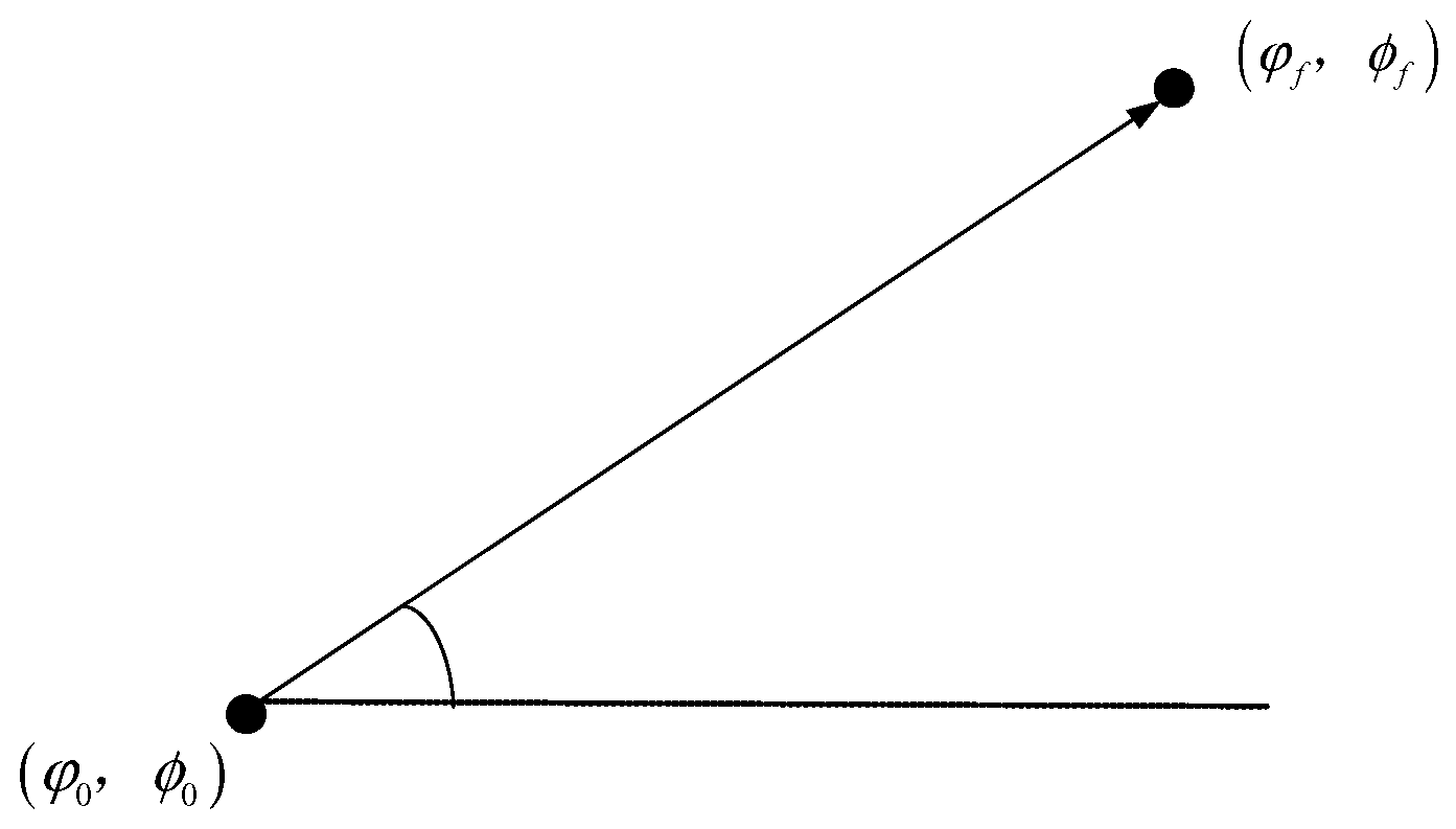
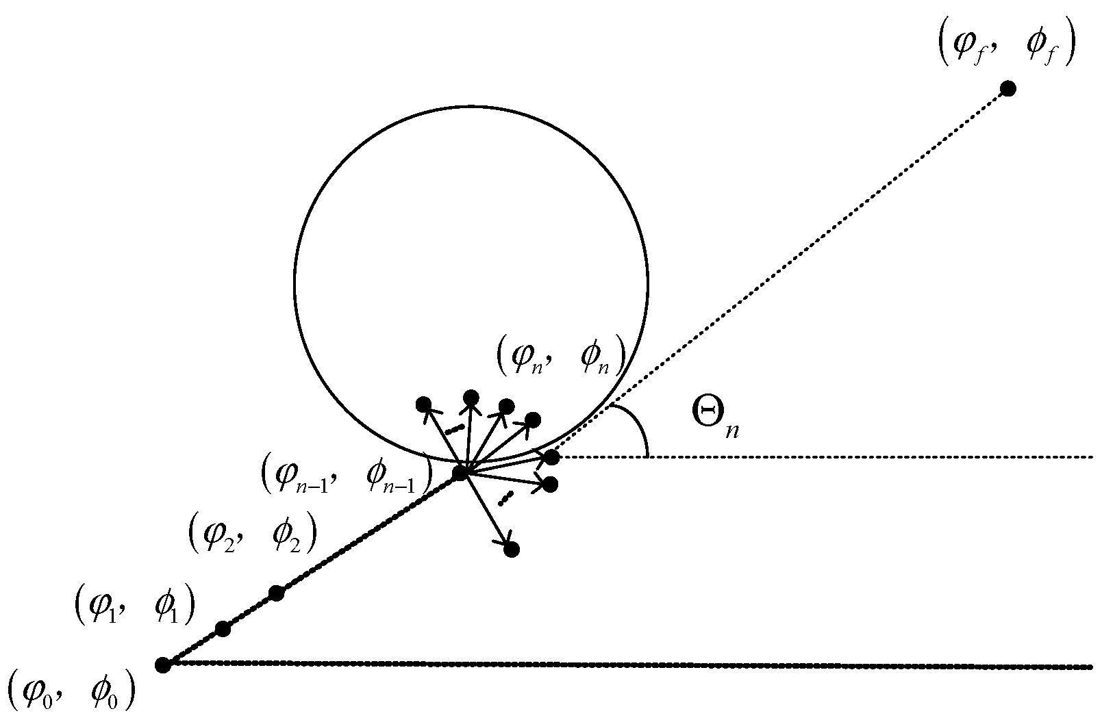
Generation of initial longitude and latitude values

The scenario studied in this paper involves a complex environment with multiple different types of NFZs. Additionally, to achieve rapid trajectory planning, the method for generating initial values should not be overly complex. A strategy for rapid initial value generation is presented below:

Step 1: According to the initial state of latitude and longitude $\left({\phi }_0,{\varphi }_0\right)$ and the terminal state $\left({\phi }_f,{\varphi }_f\right)$, an initial orientation angle ${\Theta }_0=\arctan ({\phi }_f-{\phi }_0/{\varphi }_f-{\varphi }_0)$ is determined, as shown in Figure 2.

Step 2: Taking $\left({\phi }_0,{\varphi }_0\right)$ as the starting point and ${\Theta }_0$ as the direction to advance one step to get the next node $\left({\phi }_1,{\varphi }_1\right)$, if the distance between the next node and the endpoint $\left({\phi }_f,{\varphi }_f\right)$ is less than the constant parameter h, end the algorithm and directly take $\left({\phi }_f,{\varphi }_f\right)$ as the final node $\left({\phi }_f,{\varphi }_f\right)$, then the initial latitude and longitude sequences will be obtained.

Step 3: Determine whether $\left({\phi }_1,{\varphi }_1\right)$ is in the NFZ: if it is not, take $\left({\phi }_0,{\varphi }_0\right)=\left({\phi }_1,{\varphi }_1\right)$ and turn back to Step 2; if it is, return to the previous node $\left({\phi }_{n-1},{\varphi }_{n-1}\right)$ and go to Step 4.

Step 4: At the node considered as the reference, we generate $\iota$ branches to the left and right; the angle of each branch is $\pi /2\iota$ and, at the same time, new $2\iota$ nodes are generated, then:

Step 5: Judge whether the $2\iota$ nodes are all in the NFZ; if so, discard them and go back one previous node and return to Step 4; if not, then compare those branches that are not in the NFZ with the original branches and take the node that has the smallest angle as the current node $\left({\phi }_n,{\varphi }_n\right)$, then update the directional angle ${\Theta }_n=\arctan ({\phi }_f-{\phi }_n/{\varphi }_f-{\varphi }_n)$ and return to Step 2.

The process is shown in Figure 3.

(3)

Flight path angle

Since the flight path angle is maintained at around 0° during the entry phase, a constant sequence is usually taken.

(4)

Flight heading angle

The influence of the flight heading angle on the convergence of the algorithm is mainly reflected in the starting value and the terminal value, and the linear interpolation from the starting value to the terminal value is still used.

4.3. Summary

To solve the trajectory planning problem using the convex programming method in a highly dynamic and uncertain environment, it is unavoidable that one will encounter the problems of sensitive initial value and difficult convergence of iteration, which will eventually lead to the deterioration of the solution, and this is not conducive to online trajectory generation. Compared with the research in Reference [24], this chapter concentrates on complex entry environments, proposing a variable trust region strategy and an adaptive initial value generation strategy, which greatly improves the adaptability and rapidity of the online trajectory planning algorithm. At the same time, by deriving the convexification and discretization of the corresponding optimal problems under different aircraft models, these strategies can also be used to quickly carry out online trajectory planning for other types of aircraft.

5. Results and Analysis

5.1. Algorithm Flow and Simulation Conditions

(1)

Algorithm flow

Based on the above findings, the process of solving problem P0 by using the adaptive initial value and variable trust region convex programming method is as shown in Algorithm 1:

Algorithm 1 adaptive initial value and variable trust region convex programming method

Convert the original optimal problem P0 to the convex optimal control problem P1 by convex processing and discretize P1 to get the convex programming problem P2. Initialize the initial state variables $x^{\left(0\right)}$ according to the adaptive initial value strategy. Set the scaling factor of the trust region, which is 0.9 in this example. for k = 0: 1: MaxInteration_Num:        Solve P2, get $z^{(k+1)}=\left\{x^{\left(k+1\right)};u^{\left(k+1\right)};{\vartheta }^{\left(k+1\right)};{\Phi }^{\left(k+1\right)}\right\}$        If $\left|x_i^{\left(k+1\right)}-x_i^k\right|\le \epsilon ,i=0,1,2\cdots N$:               $z_{output}=\left\{x^{\left(k+1\right)},u^{\left(k+1\right)},{\vartheta }^{\left(k+1\right)},{\Phi }^{\left(k+1\right)}\right\}$               break        else:               continue        end if end for

(2)

Simulation conditions

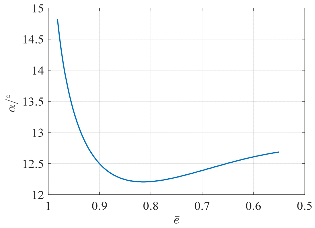
The mass of the general aviation aircraft CAV is 907.1847 kg, the reference area is 0.4837 m², the bank angle range is 0° to 165°, the maximum heating rate is 4000 kW/m², the maximum dynamic pressure is 70,000 N/m², and the maximum normal load is 2.5 g [26].

Due to the relationship between velocity $\overline{V}$ and energy $\overline{e}$, when the initial velocity and the terminal velocity are given, the entry corridor of the UAS can be obtained. We take the initial velocity V₀ = 1500 m/s and the terminal velocity V_f = 1500 m/s, and, according to Equation (18), give the velocity-height ($V-H$) entry corridor of the UAS, as shown in Figure 4.

(3)

Profile of the angle of attack

The angle of attack $\alpha$ has a huge influence on the aerodynamic parameters. In order to achieve smooth flight and ensure that the algorithm can converge smoothly, the nominal angle of attack is used in this paper, which can be expressed as an empirical function related to the dimensionless energy $\overline{e}$:

$$\alpha =43.29{\overline{e}}^5-155.8{\overline{e}}^4+223.6{\overline{e}}^3-159.8{\overline{e}}^2+56.84\overline{e}-7.814$$

(46)

From Equation (46), the angle of attack profile can be obtained as shown in Figure 5.

(4)

Parameter setting

The simulation verification in this paper is carried out on a MECHREVO 16k laptop with an AMD R7-7735H CPU @ 3.20 GHz. In the simulation experiment, the convex programming with adaptive initial value strategy is referred to as Method 1 and the convex programming with adaptive initial value strategy and variable trust region strategy is referred to as Method 2.

The initial and terminal conditions of the entry phase are shown in

Table 1. The initial and final conditions of the entry phase.

State Variables	Initial Condition	Terminal Condition
height/m	54,000	23,000
longitude/°	130	233.3
latitude/°	−35	53.3
velocity/(m·s−1)	7500	1500
flight path angle/°	0	0
flight heading angle/°	45.12	50

:

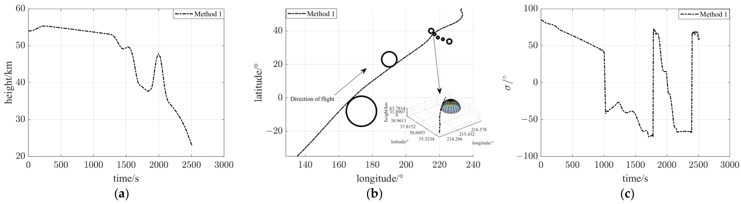
5.2. Analysis of Simulation Results for Method 1

To verify the effectiveness of the adaptive initial value strategy, this subsection gives the parameters of two types of different NFZs required for the simulation, where the centers of the spherical NFZs are on the ground, that is, the geocentric distance of the spherical center is $R_0$. The parameters of cylindrical NFZs are shown in

Table 2. Parameters of the cylindrical NFZs for UAS entry.

Longitude/°	Latitude/°	Radius/km
173	−8	1000.5
210	8	501

, and those of spherical NFZs are shown in

Table 3. Parameters of the spherical NFZs for UAS entry.

Longitude/°	Latitude/°	Radius/km
219	36	80
217	38	80
222	35	80
215	40	160
226	33.7	160

.

According to the above initial values and the parameters of the NFZs, the results of the initial values of adaptive latitude and longitude are first given as shown in Figure 6:

Then, the above result is used as the initial value of the convex programming to solve, and the simulation results are shown in Figure 7.

It can be seen from the figures that when there are NFZs, due to the restriction of the performance index of the shortest entry time, the UAS adopts the strategy of flying along the boundary of the NFZs.

Around 1700 s and 2400 s, the UAS achieved the circumvention of two NFZs by rapid bank reversals, while adjusting its flight height to meet the dynamic pressure constraint q, which is expressed in Equation (18). The traditional bank angle control strategy often uses the heading deviation as the basis for determining the sign of the bank angle, under which the phenomenon of bank reversal is frequent. Within the framework of convex programming, even if the variation law of the bank angle is not set, the optimal solution of the proposed method automatically converges to the trajectory corresponding to the bank reversal control curve. By adjusting the sign of the bank angle, the algorithm achieves a fast response to the NFZs and adjusts the flight height to meet the constraints of the entry corridor.

Considering the situation of complex NFZs, with the increase in NFZs, the computational burden will also increase. Under the parameters given above, the use of linear initial values will directly lead to the infeasibility of the algorithm. The adaptive initial value solves this problem well by introducing the adaptive initial value; the algorithm converges after 50 iterations, and it takes about 40.17 s.

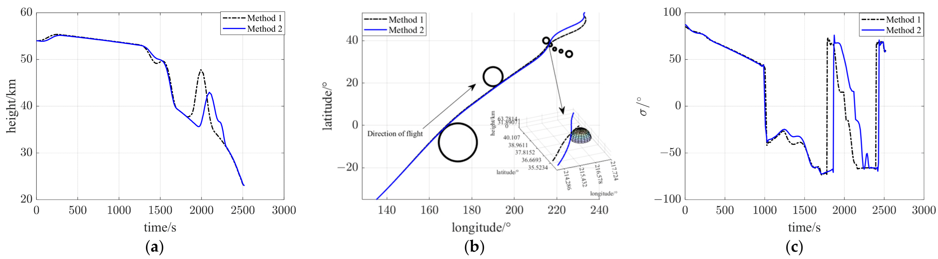
5.3. Analysis of Simulation Results for Method 2

While the adaptive initial values designed in previous sections have made the algorithm feasible, they still require many iterations to converge. This paper enhances the convergence speed of the algorithm by updating the trust region. The simulation results are shown in Figure 8 and Figure 9, and

Table 4. Comparison of different solutions.

Solution	Total Entry Time/s	Solving Time/s	Iteration Number
Normal convex programming	not feasible	not feasible	not feasible
Method 1	2518.6796	40.17	50
Method 2	2521.4330	18.37	21

:

The figures show that when the variable trust region strategy is adopted, the change in the height profile is smoother, which is more conducive to UAS flight.

In the meantime, the convergence of Method 2 only takes 21 iterations and about 18.37 s, which is a 54.27% improvement in time over Method 1. The relative error of the performance index of Method 2 and Method 1 is not more than 0.109%.

6. Conclusions

In order to solve the problem of long durations and the difficult convergence of UAS online trajectory planning, this paper proposes an approach to entrance trajectory optimization based on adaptive initial values in the variable trust region convex programming framework. To simulate the complex flight environment, a number of spherical and cylindrical NFZs were designed, and the adaptive initial value strategy and the variable trust region strategy were introduced into the traditional convex programming algorithm to realize the fast online generation of trajectories. Simulations have validated that when traditional linear initial values fail to provide a solution, the adaptive initial values effectively address this issue. Additionally, a variable-trust-region strategy was incorporated to prevent the algorithm from iterating continually near the optimal solution. Simulation results indicate that the variable-trust-region strategy accelerates the convergence speed of the algorithm by 54.27%, significantly enhancing its optimization capabilities and meeting the requirements of online trajectory planning.

The proposed algorithm framework is based on the convex programming method, which can simplify the solution process and has strong adaptability to the trajectory optimization problems of other types of aircraft. However, the proposed algorithm still has some limitations, such as the problem that the dynamic responses of system states are often neglected in the proposed algorithm. In follow-up research, in addition to considering more detailed modeling of the environment and aircraft, tracking guidance law and a flight controller for fast trajectory generation are also important development directions.

References

1. Liu, S.; Yan, B.; Huang, W.; Zhang, X.; Yan, J. Current status and prospects of terminal guidance laws for intercepting hypersonic vehicles in near space: A review. J. Zhejiang Univ.-Sci. A 2023, 24, 387–403. [Google Scholar] [CrossRef]
2. Liu, S.; Lin, Z.; Wang, Y.; Huang, W.; Yan, B.; Li, Y. Three-body cooperative active defense guidance law with overload constraints: A small speed ratio perspective. Chin. J. Aeronaut. 2025, 38, 103171. [Google Scholar] [CrossRef]
3. Williams, P. Hermite-legendre-gauss-lobatto direct transcription in trajectory optimization. J. Guid. Control Dyn. 2009, 32, 1392–1395. [Google Scholar] [CrossRef]
4. Darby, C.L.; Hager, W.W.; Rao, A.V. An hp-adaptive pseudospectral method for solving optimal control problems. Optim. Control Appl. Methods 2011, 32, 476–502. [Google Scholar] [CrossRef]
5. Song, X.; Yao, X.; Ye, S. Trajectory Optimization of Small Supersonic UAV Based on Pseudospectral Method. J. ZheJiang Univ. (Eng. Sci.) 2022, 56, 193–201. (In Chinese) [Google Scholar] [CrossRef]
6. Cai, G.; Liu, Z.; Luo, K.; Guan, F. Trajectory Optimization of Near-Space Variable-Wing Aircraft Based on Improved Pseudospectral Method. Aerosp. Technol. 2022, 5, 45–57. (In Chinese) [Google Scholar] [CrossRef]
7. Mu, L.; Cao, S.; Wang, B.; Zhang, Y.; Feng, N.; Li, X. Pseudospectral-Based Rapid Trajectory Planning and Feedforward Linearization Guidance. Drones 2024, 8, 371. [Google Scholar] [CrossRef]
8. Benedikter, B.; Zavoli, A.; Colasurdo, G. A Convex Optimization Approach for Finite-Thrust Time-Constrained Cooperative Rendezvous. Astrodyn. Spec. Conf. 2019, 171, 1483–1498. [Google Scholar] [CrossRef]
9. Lu, P.; Liu, X. Autonomous Trajectory Planning for Rendezvous and Proximity Operations by Conic Optimization. J. Guid. Control Dyn. 2013, 36, 375–389. [Google Scholar] [CrossRef]
10. Morgan, D.; Chung, S.; Hadaegh, F. Model Predictive Control of Swarms of Spacecraft Using Sequential Convex Programming. J. Guid. Control Dyn. 2014, 37, 1725–1740. [Google Scholar] [CrossRef]
11. Foust, R.; Chung, S.; Hadaegh, F. Optimal Guidance and Control with Nonlinear Dynamics Using Sequential Convex Programming. J. Guid. Control Dyn. 2019, 43, 633–644. [Google Scholar] [CrossRef]
12. Szmuk, M.; Acikmese, B.; Berning, A. Successive Convexification for Fuel-Optimal Powered Landing with Aerodynamic Drag and Non-Convex Constraints. In Proceedings of the AIAA Guidance, Navigation, and Control Conference, San Diego, CA, USA, 4–8 January 2016. [Google Scholar] [CrossRef]
13. Liu, X. Fuel-Optimal Rocket Landing with Aerodynamic Controls. J. Guid. Control Dyn. 2019, 42, 65–77. [Google Scholar] [CrossRef]
14. Pinson, R.; Lu, P. Rapid Generation of Optimal Asteroid Powered Descent Trajectories via Convex Optimization. In Proceedings of the AAS/AIAA Astrodynamics Specialist Conference, Vail, CO, USA, 10–13 August 2015. [Google Scholar] [CrossRef]
15. Liu, X.; Shen, Z.; Lu, P. Solving the maximum-crossrange problem via successive second-order cone programming with a line search. Aerosp. Sci. Technol. 2015, 47, 10–20. [Google Scholar] [CrossRef]
16. Liu, X.; Shen, Z.; Lu, P. Entry Trajectory Optimization by Second-Order Cone Programming. J. Guid. Control Dyn. 2016, 39, 227–241. [Google Scholar] [CrossRef]
17. Zhao, D.; Song, Z. Reentry trajectory optimization with waypoint and no-fly zone constraints using multiphase convex programming. Acta Astronaut. 2017, 137, 60–69. [Google Scholar] [CrossRef]
18. Song, R.; Zhu, Y.; Xu, G.; Sun, J.; Long, T. Cooperative Reentry Trajectory Planning for Hypersonic Vehicles Based on Sequential Convex Optimization. Tactical Missile Technol. 2020, 6, 7–16. (In Chinese) [Google Scholar] [CrossRef]
19. Sagliano, M.; Mooij, E. Optimal drag-energy entry guidance via pseudospectral convex optimization. Aerosp. Sci. Technol. 2021, 117, 106946. [Google Scholar] [CrossRef]
20. Sun, Y. Trajectory Optimization and Guidance of Hypersonic Vehicle Based on Improved Gauss Pseudospectral Method. Ph.D. Thesis, Harbin Institute of Technology, Harbin, China, 2012. (In Chinese). [Google Scholar]
21. Yang, F.; Gong, Z.; Wei, Q.; Lei, Y. Secure Containment Control for Multi-UAV Systems by Fixed-Time Convergent Reinforcement Learning. IEEE Trans. Cybern. 2025, 1–14. [Google Scholar] [CrossRef]
22. Gong, Z.; Yang, F. Secure tracking control via fixed-time convergent reinforcement learning for a UAV CPS. IEEE/CAA J. Autom. Sin. 2024, 11, 1699–1701. [Google Scholar] [CrossRef]
23. Luo, Y.; Wang, J.; Jiang, J.; Liang, H. Reentry trajectory planning for hypersonic vehicles via an improved sequential convex programming method. Aerosp. Sci. Technol. 2024, 149, 109130. [Google Scholar] [CrossRef]
24. Dai, P.; Feng, D.; Feng, W.; Cui, J.; Zhang, L. Entry trajectory optimization for hypersonic vehicles based on convex programming and neural network. Aerosp. Sci. Technol. 2023, 137, 108259. [Google Scholar] [CrossRef]
25. Zong, Q.; Li, Z.; Ye, L.; Tian, B. Online reconstruction of RLV reentry trajectory with variable trust domain sequence convex programming. J. Harbin Inst. Technol. 2020, 52, 147–155. (In Chinese) [Google Scholar]
26. Phillips, T. A Common Aero Vehicle (CAV) Model, Description, and Employment Guide; Schafer Corp. for Air Force Research Lab and Air Force Space Command: Greene County, OH, USA, 2003. [Google Scholar]
Figure 1. Flowchart of the variable trust region strategy.
Drones 09 00210 g001
Figure 2. Definition of the angle of bearing.
Drones 09 00210 g002
Figure 3. Evenly generated branches.
Drones 09 00210 g003
Figure 4. V-H corridor for UAS entry.
Drones 09 00210 g004
Figure 5. Angle of attack—dimensionless energy profile.
Drones 09 00210 g005
Figure 6. Adaptive latitude and longitude initial value generation.
Drones 09 00210 g006
Figure 7. (a) Time-height curve using Method1; (b) longitude-latitude curve using Method1; (c) time-bank angle curve using Method1.
Drones 09 00210 g007
Figure 8. (a) Time-height curve using Method1 and Method2; (b) longitude-latitude curve using Method1 and Method2; (c) time-bank angle curve using Method1 and Method2.
Drones 09 00210 g008
Figure 9. (a) Time-CL curve using Method2; (b) time-CD curve using Method2.
Drones 09 00210 g009