
A Low-Latency Dynamic Object Detection Algorithm Fusing Depth and Events


Abstract
1. Introduction
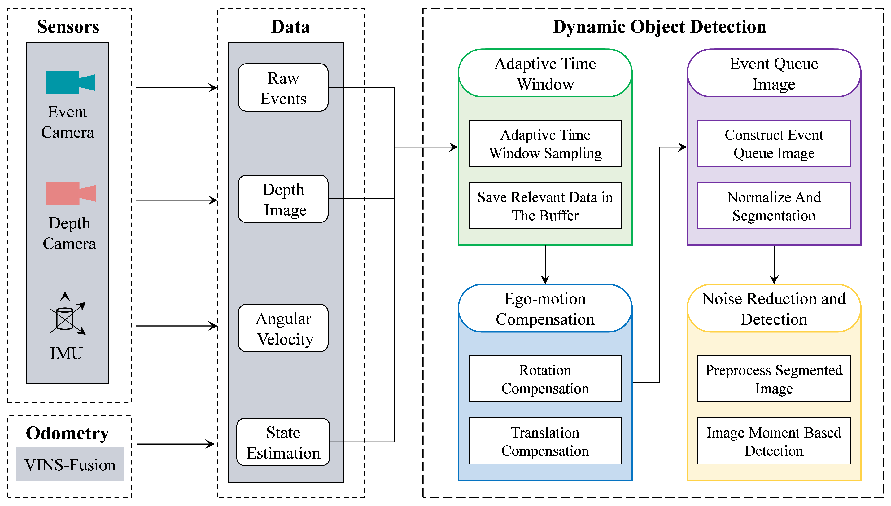
- The authors design a strategy to adaptively select the size of the time window for event processing based on the motion within a scene. This approach more effectively balances the signal-to-noise ratio and latency compared to using a fixed time window.
- The authors propose an ego-motion compensation algorithm to eliminate events caused by the camera’s ego-motion while retaining events generated by the objects.
- The authors construct a “First in, First out” event queue and perform detection on its derivative, which helps reduce computational complexity.
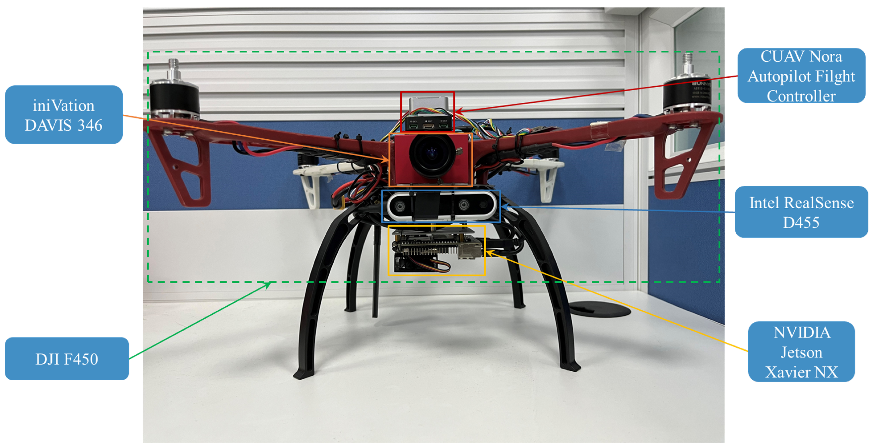
- The authors construct a completed obstacle avoidance pipeline and deploy it on a custom-built quadrotor for validation in a real environment.
2. Related Work
3. Obstacle Detection
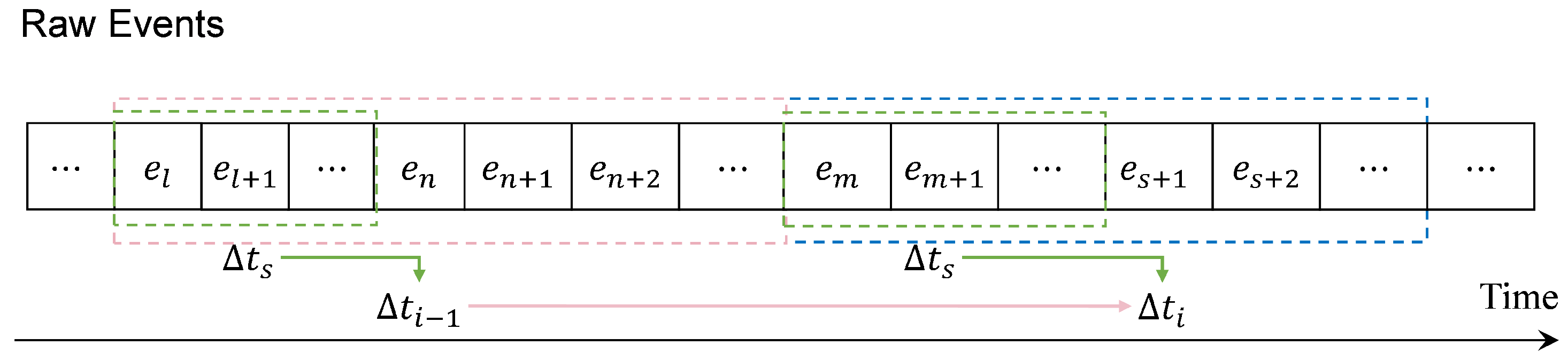
3.1. Adaptive Time Window
3.2. Ego-Motion Compensation
3.3. Event Queue Image
3.4. Noise Reduction and Detection
| Algorithm 1 Detection |
| Require: , . |
| Ensure: . |
|
4. Obstacle Avoidance
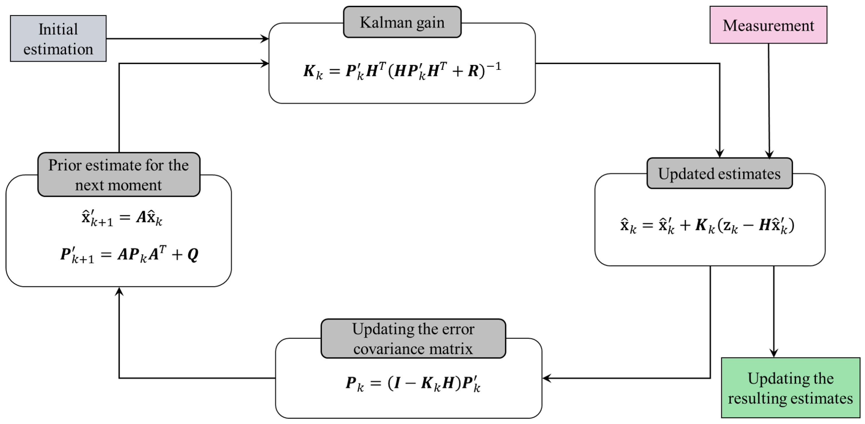
4.1. Obstacle Position Estimation
4.2. Obstacle Velocity Estimation
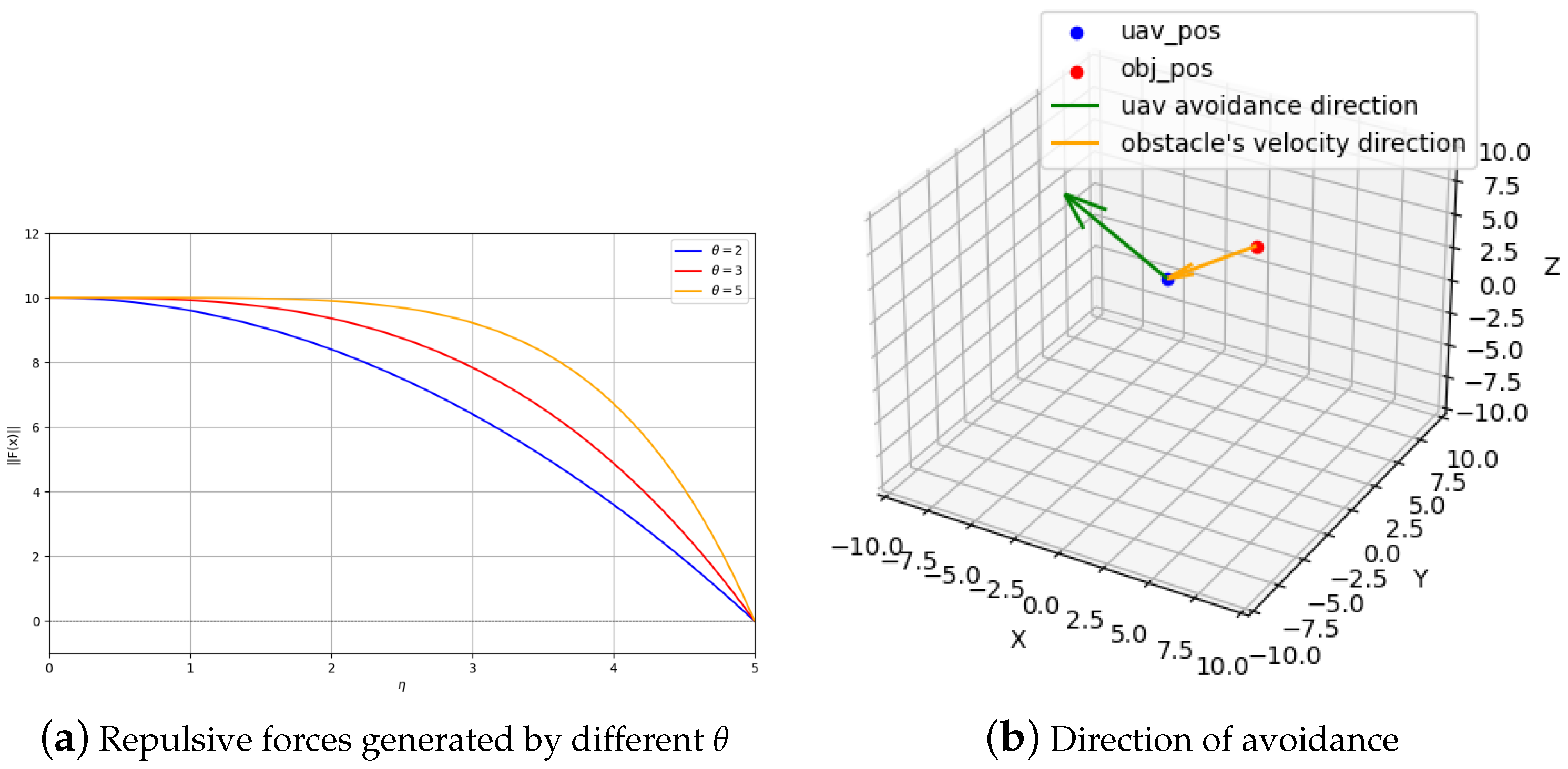
4.3. Artificial Repulsive Field
5. Experiments
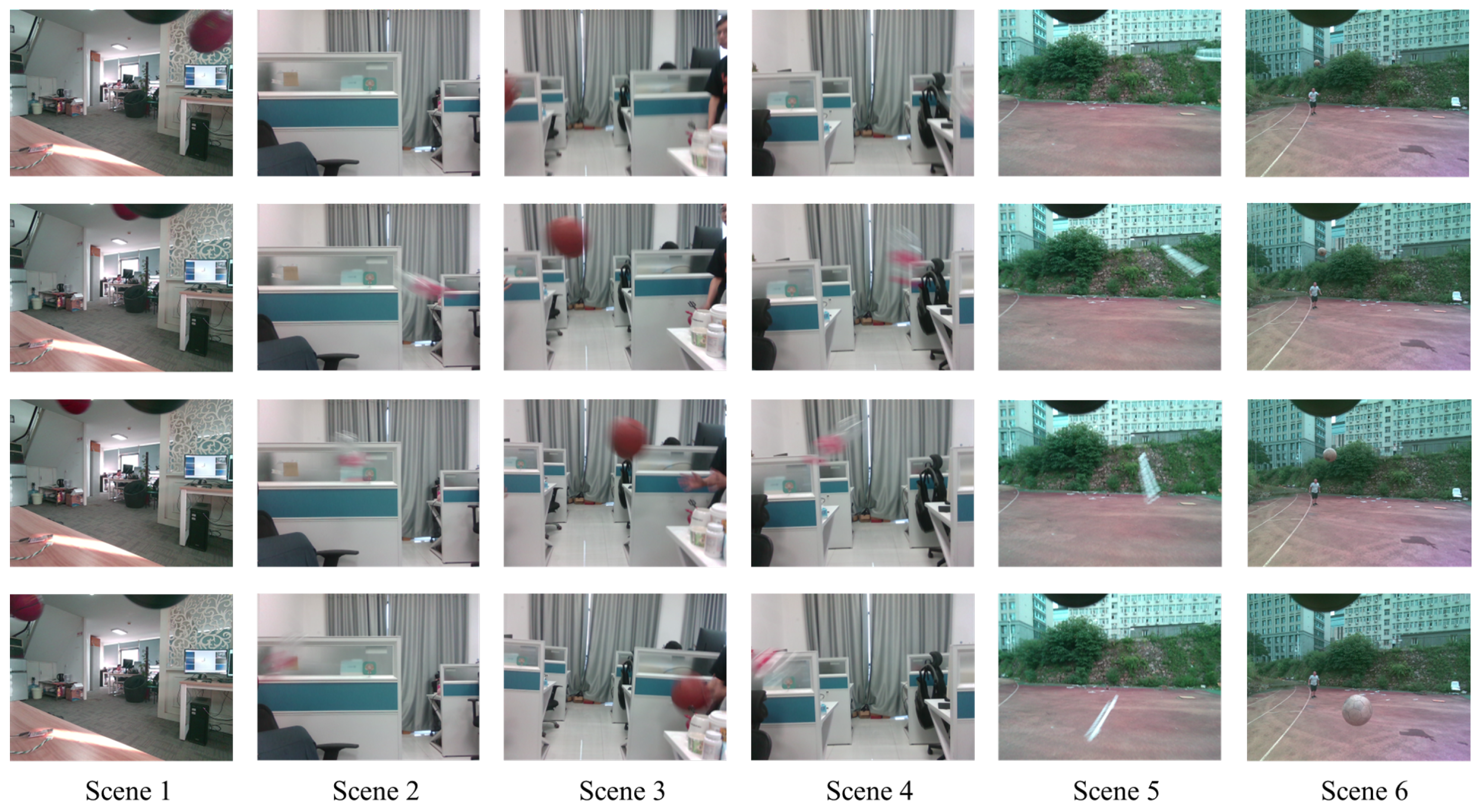
5.1. Datasets
5.2. Results and Analysis
5.2.1. Time Cost of Constructing Event Images
5.2.2. Performance Comparison of Detection
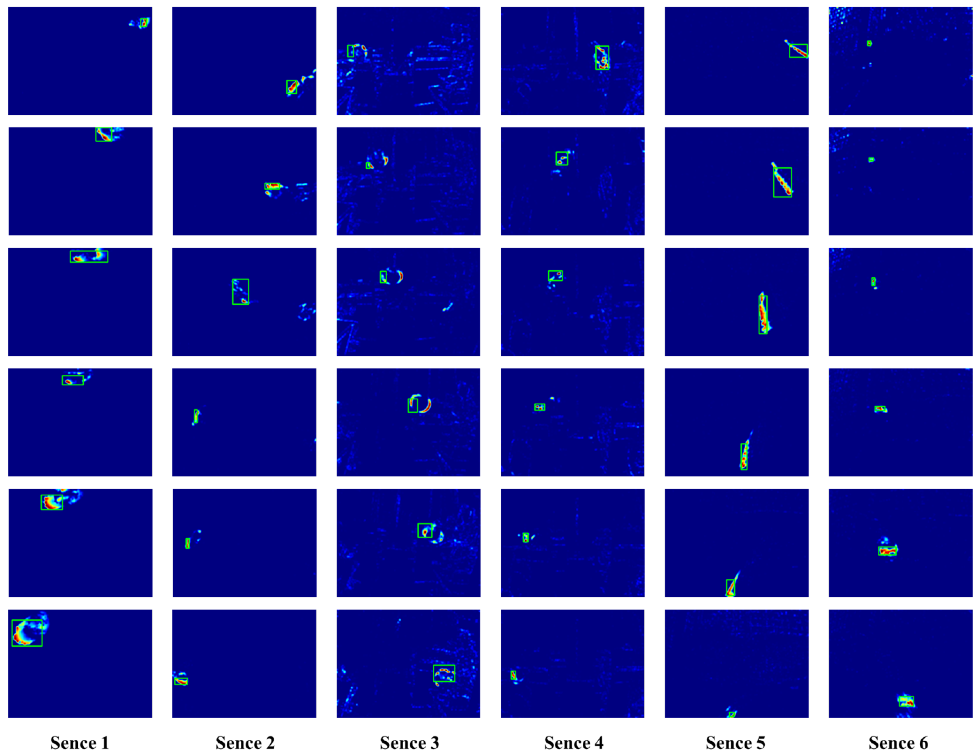
5.2.3. Accuracy of Moving Object Detection
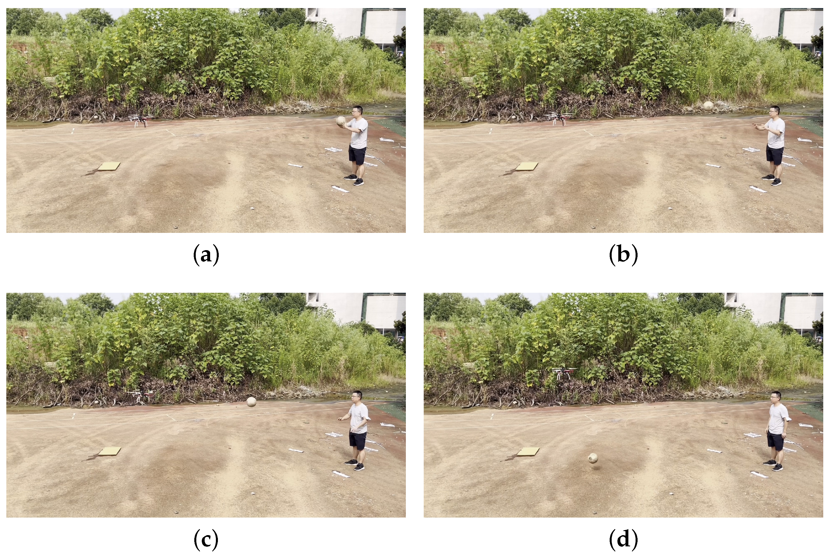
5.2.4. Obstacle Avoidance Test in a Real Environment
6. Conclusions
Author Contributions
Funding
Data Availability Statement
Conflicts of Interest
References
- Huang, G. Visual-inertial navigation: A concise review. In Proceedings of the 2019 International Conference on Robotics and Automation (ICRA), Montreal, QC, Canada, 20–24 May 2019; pp. 9572–9582. [Google Scholar]
- Falanga, D.; Kleber, K.; Scaramuzza, D. Dynamic obstacle avoidance for quadrotors with event cameras. Sci. Robot. 2020, 5, eaaz9712. [Google Scholar] [CrossRef] [PubMed]
- Rodríguez-Gómez, J.P.; Tapia, R.; Garcia, M.d.M.G.; Martínez-de Dios, J.R.; Ollero, A. Free as a bird: Event-based dynamic sense-and-avoid for ornithopter robot flight. IEEE Robot. Autom. Lett. 2022, 7, 5413–5420. [Google Scholar] [CrossRef]
- Forrai, B.; Miki, T.; Gehrig, D.; Hutter, M.; Scaramuzza, D. Event-based agile object catching with a quadrupedal robot. In Proceedings of the 2023 IEEE International Conference on Robotics and Automation (ICRA), London, UK, 29 May–2 June 2023; pp. 12177–12183. [Google Scholar]
- Falanga, D.; Kim, S.; Scaramuzza, D. How fast is too fast? the role of perception latency in high-speed sense and avoid. IEEE Robot. Autom. Lett. 2019, 4, 1884–1891. [Google Scholar] [CrossRef]
- Posch, C.; Serrano-Gotarredona, T.; Linares-Barranco, B.; Delbruck, T. Retinomorphic event-based vision sensors: Bioinspired cameras with spiking output. Proc. IEEE 2014, 102, 1470–1484. [Google Scholar] [CrossRef]
- Gallego, G.; Delbrück, T.; Orchard, G.; Bartolozzi, C.; Taba, B.; Censi, A.; Leutenegger, S.; Davison, A.J.; Conradt, J.; Daniilidis, K.; et al. Event-Based Vision: A Survey. IEEE Trans. Pattern Anal. Mach. Intell. 2022, 44, 154–180. [Google Scholar] [CrossRef] [PubMed]
- He, B.; Li, H.; Wu, S.; Wang, D.; Zhang, Z.; Dong, Q.; Xu, C.; Gao, F. Fast-dynamic-vision: Detection and tracking dynamic objects with event and depth sensing. In Proceedings of the 2021 IEEE/RSJ International Conference on Intelligent Robots and Systems (IROS), Prague, Czech Republic, 27 September–1 October 2021; pp. 3071–3078. [Google Scholar]
- Gallego, G.; Rebecq, H.; Scaramuzza, D. A unifying contrast maximization framework for event cameras, with applications to motion, depth, and optical flow estimation. In Proceedings of the IEEE Conference on Computer Vision and Pattern Recognition, Salt Lake City, UT, USA, 18–22 June 2018; pp. 3867–3876. [Google Scholar]
- Stoffregen, T.; Kleeman, L. Event cameras, contrast maximization and reward functions: An analysis. In Proceedings of the IEEE/CVF Conference on Computer Vision and Pattern Recognition, Long Beach, CA, USA, 15–20 June 2019; pp. 12300–12308. [Google Scholar]
- Liu, H.; Moeys, D.P.; Das, G.; Neil, D.; Liu, S.C.; Delbrück, T. Combined frame-and event-based detection and tracking. In Proceedings of the 2016 IEEE International Symposium on Circuits and systems (ISCAS), Montreal, QC, Canada, 22–25 May 2016; pp. 2511–2514. [Google Scholar]
- Iacono, M.; Weber, S.; Glover, A.; Bartolozzi, C. Towards event-driven object detection with off-the-shelf deep learning. In Proceedings of the 2018 IEEE/RSJ International Conference on Intelligent Robots and Systems (IROS), Madrid, Spain, 1–5 October 2018; pp. 1–9. [Google Scholar]
- Tomy, A.; Paigwar, A.; Mann, K.S.; Renzaglia, A.; Laugier, C. Fusing event-based and rgb camera for robust object detection in adverse conditions. In Proceedings of the 2022 International Conference on Robotics and Automation (ICRA), Philadelphia, PA, USA, 23–27 May 2022; pp. 933–939. [Google Scholar]
- Gehrig, M.; Scaramuzza, D. Recurrent vision transformers for object detection with event cameras. In Proceedings of the IEEE/CVF Conference on Computer Vision and Pattern Recognition, Vancouver, BC, Canada, 17–24 June 2023; pp. 13884–13893. [Google Scholar]
- Gallego, G.; Gehrig, M.; Scaramuzza, D. Focus is all you need: Loss functions for event-based vision. In Proceedings of the IEEE/CVF Conference on Computer Vision and Pattern Recognition, Long Beach, CA, USA, 15–20 June 2019; pp. 12280–12289. [Google Scholar]
- Peng, X.; Gao, L.; Wang, Y.; Kneip, L. Globally-optimal contrast maximisation for event cameras. IEEE Trans. Pattern Anal. Mach. Intell. 2021, 44, 3479–3495. [Google Scholar] [CrossRef] [PubMed]
- Shiba, S.; Klose, Y.; Aoki, Y.; Gallego, G. Secrets of Event-based Optical Flow, Depth and Ego-motion Estimation by Contrast Maximization. IEEE Trans. Pattern Anal. Mach. Intell. 2024, 46, 7742–7759. [Google Scholar] [CrossRef] [PubMed]
- Paredes-Vallés, F.; Scheper, K.Y.; De Croon, G.C. Unsupervised learning of a hierarchical spiking neural network for optical flow estimation: From events to global motion perception. IEEE Trans. Pattern Anal. Mach. Intell. 2019, 42, 2051–2064. [Google Scholar] [CrossRef] [PubMed]
- Gallego, G.; Scaramuzza, D. Accurate angular velocity estimation with an event camera. IEEE Robot. Autom. Lett. 2017, 2, 632–639. [Google Scholar] [CrossRef]
- Kim, H.; Kim, H.J. Real-time rotational motion estimation with contrast maximization over globally aligned events. IEEE Robot. Autom. Lett. 2021, 6, 6016–6023. [Google Scholar] [CrossRef]
- Stoffregen, T.; Gallego, G.; Drummond, T.; Kleeman, L.; Scaramuzza, D. Event-based motion segmentation by motion compensation. In Proceedings of the IEEE/CVF International Conference on Computer Vision, Seoul, Republic of Korea, 27–28 October 2019; pp. 7244–7253. [Google Scholar]
- Zhou, Y.; Gallego, G.; Lu, X.; Liu, S.; Shen, S. Event-based motion segmentation with spatio-temporal graph cuts. IEEE Trans. Neural Networks Learn. Syst. 2021, 34, 4868–4880. [Google Scholar] [CrossRef] [PubMed]
- Mondal, A.; Giraldo, J.H.; Bouwmans, T.; Chowdhury, A.S. Moving object detection for event-based vision using graph spectral clustering. In Proceedings of the IEEE/CVF International Conference on Computer Vision, Montreal, BC, Canada, 11–17 October 2021; pp. 876–884. [Google Scholar]
- Mitrokhin, A.; Fermüller, C.; Parameshwara, C.; Aloimonos, Y. Event-based moving object detection and tracking. In Proceedings of the 2018 IEEE/RSJ International Conference on Intelligent Robots and Systems (IROS), Madrid, Spain, 1–5 October 2018; pp. 1–9. [Google Scholar]
- Qin, T.; Li, P.; Shen, S. Vins-mono: A robust and versatile monocular visual-inertial state estimator. IEEE Trans. Robot. 2018, 34, 1004–1020. [Google Scholar] [CrossRef]
- Kalman, R.E. A new approach to linear filtering and prediction problems. J. Basic Eng. 1960, 82, 35–45. [Google Scholar] [CrossRef]
- Khatib, O. Real-time obstacle avoidance for manipulators and mobile robots. Int. J. Robot. Res. 1986, 5, 90–98. [Google Scholar] [CrossRef]
- Ester, M.; Kriegel, H.P.; Sander, J.; Xu, X. A density-based algorithm for discovering clusters in large spatial databases with noise. In Proceedings of the KDD, Portland, OR, USA, 2–4 August 1996; Volume 96, pp. 226–231. [Google Scholar]


| Name | Software Dependency | Version |
|---|---|---|
| VINS-Fusion | Cmake | 3.22.1 |
| Ceres Solver | 2.0.0 | |
| Eigen | 3.3.7 | |
| PX4 | python | 3.9.13 |
| OpenCV | 4.2.0 | |
| make | 4.1 | |
| gazebo | 9.0 |
| Topic | Frequency | Data Format |
|---|---|---|
| /dvs/events | - | dvs_msgs/EventArray |
| /mavros/imu/data | 190 | sensor_msgs/Imu |
| /camera/color/image_raw | 30 | sensor_msgs/Image |
| /camera/depth/image_rect_raw | 45 | sensor_msgs/Image |
| /vins_fusion/odometry | 15 | nav_msgs/Odometry |
| Indicators | Methods | Scene 1 | Scene 2 | Scene 3 | Scene 4 | Scene 5 | Scene 6 |
|---|---|---|---|---|---|---|---|
| (ms) | Ours | 0.12 | 0.12 | 0.17 | 0.11 | 0.17 | 0.18 |
| Falanga | 0.03 | 0.07 | 0.28 | 0.29 | 0.06 | 0.23 | |
| FAST | 0.22 | 0.19 | 0.39 | 0.41 | 0.25 | 0.26 | |
| (ms) | Ours | 0.15 | 0.32 | 0.43 | 0.32 | 0.52 | 0.48 |
| Falanga | 0.07 | 0.24 | 0.67 | 0.47 | 0.37 | 0.51 | |
| FAST | 0.27 | 0.49 | 0.89 | 0.68 | 0.69 | 0.59 | |
| (ms) | Ours | 0.82 | 0.83 | 1.85 | 1.94 | 0.91 | 1.15 |
| Falanga | 0.33 | 0.55 | 1.27 | 0.96 | 0.63 | 0.67 | |
| FAST | 0.48 | 1.35 | 1.57 | 1.24 | 1.11 | 0.73 | |
| (ms) | Ours | 8.79 | 9.42 | 26.25 | 18.86 | 17.34 | 28.86 |
| Falanga | 3.92 | 4.79 | 28.29 | 21.39 | 10.35 | 30.07 | |
| FAST | 16.36 | 17.63 | 52.98 | 40.97 | 23.41 | 33.24 |
| Scene | Methods | Running Time (ms) | The Relative Contrast (%) | |||||
|---|---|---|---|---|---|---|---|---|
| Scene 1 | Ours | 0.73 | 0.92 | 2.85 | 55.59 | 22.7 | 81.9 | 100 |
| Falanga | 0.82 | 1.18 | 2.14 | 62.83 | 26.4 | 70.1 | 100 | |
| FAST | 0.97 | 1.25 | 2.52 | 75.24 | 29.1 | 75.3 | 100 | |
| Scene 2 | Ours | 0.69 | 0.91 | 3.19 | 56.05 | 19.2 | 71.8 | 95.6 |
| Falanga | 0.88 | 0.98 | 2.59 | 59.91 | 23.9 | 51.2 | 97.6 | |
| FAST | 0.91 | 1.23 | 2.74 | 75.53 | 26.8 | 60.4 | 100 | |
| Scene 3 | Ours | 0.95 | 1.37 | 2.61 | 83.31 | 0.7 | 27.1 | 54.2 |
| Falanga | 1.04 | 1.59 | 3.62 | 89.23 | 3.8 | 18.7 | 45.1 | |
| FAST | 1.19 | 1.85 | 2.47 | 112.9 | 4.3 | 20.6 | 48.9 | |
| Scene 4 | Ours | 0.84 | 1.18 | 4.62 | 71.32 | 4.3 | 27.5 | 52.9 |
| Falanga | 0.95 | 1.35 | 4.36 | 81.28 | 6.2 | 14.6 | 35.5 | |
| FAST | 1.12 | 1.59 | 3.17 | 95.59 | 7.4 | 16.9 | 43.4 | |
| Scene 5 | Ours | 1.02 | 1.28 | 2.09 | 78.86 | 8.9 | 35.1 | 94.2 |
| Falanga | 1.17 | 1.39 | 1.61 | 80.59 | 10.4 | 25.9 | 80.3 | |
| FAST | 1.21 | 1.53 | 1.74 | 83.27 | 12.1 | 30.2 | 90.5 | |
| Scene 6 | Ours | 1.03 | 1.40 | 3.55 | 83.96 | 8.5 | 29.7 | 59.6 |
| Falanga | 1.21 | 1.56 | 3.61 | 90.18 | 9.1 | 20.2 | 40.5 | |
| FAST | 1.57 | 1.69 | 2.47 | 87.55 | 9.3 | 26.9 | 54.1 | |
| Method | Indicators | Scene 1 | Scene 2 | Scene 3 | Scene 4 | Scene 5 | Scene 6 |
|---|---|---|---|---|---|---|---|
| Ours | 14 | 20 | 18 | 16 | 13 | 25 | |
| 93% | 90% | 85% | 75% | 92% | 73% | ||
| Falanga | 16 | 24 | 20 | 16 | 15 | 28 | |
| 89% | 85% | 70% | 67% | 85% | 64% | ||
| FAST | 16 | 24 | 20 | 16 | 15 | 28 | |
| 92% | 89% | 80% | 75% | 82% | 68% |
Disclaimer/Publisher’s Note: The statements, opinions and data contained in all publications are solely those of the individual author(s) and contributor(s) and not of MDPI and/or the editor(s). MDPI and/or the editor(s) disclaim responsibility for any injury to people or property resulting from any ideas, methods, instructions or products referred to in the content. |
© 2025 by the authors. Licensee MDPI, Basel, Switzerland. This article is an open access article distributed under the terms and conditions of the Creative Commons Attribution (CC BY) license (https://creativecommons.org/licenses/by/4.0/).
Share and Cite
Chen, D.; Zhou, L.; Guo, C. A Low-Latency Dynamic Object Detection Algorithm Fusing Depth and Events. Drones 2025, 9, 211. https://doi.org/10.3390/drones9030211
Chen D, Zhou L, Guo C. A Low-Latency Dynamic Object Detection Algorithm Fusing Depth and Events. Drones. 2025; 9(3):211. https://doi.org/10.3390/drones9030211
Chicago/Turabian StyleChen, Duowen, Liqi Zhou, and Chi Guo. 2025. "A Low-Latency Dynamic Object Detection Algorithm Fusing Depth and Events" Drones 9, no. 3: 211. https://doi.org/10.3390/drones9030211
APA StyleChen, D., Zhou, L., & Guo, C. (2025). A Low-Latency Dynamic Object Detection Algorithm Fusing Depth and Events. Drones, 9(3), 211. https://doi.org/10.3390/drones9030211