Article

Multi-Object Tracking with Distributed Drones’ RGB Cameras Considering Object Localization Uncertainty

1
Unmanned System Research Institute, National Key Laboratory of Unmanned Aerial Vehicle Technology, Integrated Research and Development Platform of Unmanned Aerial Vehicle Technology, Northwestern Polytechnical University, Xi’an 710072, China
2
Shanghai Electro-Mechanical Engineering Institute, Shanghai 201109, China
3
Xi’an Jingwei Sensing Technology Co., Ltd., Xi’an 710000, China
*
Author to whom correspondence should be addressed.
Drones 2025, 9(12), 867; https://doi.org/10.3390/drones9120867
Submission received: 17 October 2025 / Revised: 7 December 2025 / Accepted: 11 December 2025 / Published: 16 December 2025

Highlights

What are the main findings?
  • A comprehensive passive sensing framework for multi-object tracking with distributed drones is presented. The robust localization and tracking of aerial objects can be achieved by exploiting spatio-temporal information to associate targets detected by different views.
  • Object localization uncertainty is modeled in the Kalman filter through carefully designed process and observation noise covariance matrices. The resulting data association, based on the Mahalanobis distance, enhances the performance of multi-object tracking.
What are the implications of the main finding?
  • Since aerial objects are always small and share similar appearance features, data association between different viewpoints of passive sensors needs to consider more about the geometric constraints and temporal information.
  • The motion of the observer drone necessitates refined modeling of process and observation noise to achieve robust object tracking.

Abstract

Reliable 3D multi-object tracking (MOT) using distributed drones remains challenging due to the lack of active sensing and the ambiguity in associating detections from different views. This paper presents a passive sensing framework that integrates multi-view data association and 3D MOT for aerial objects. First, object localization is achieved via triangulation using two onboard RGB cameras. To mitigate false positive objects caused by crossing bearings, spatial–temporal cues derived from 2D image detections and tracking results are exploited to establish a likelihood-based association matrix, enabling robust multi-view data association. Subsequently, optimized process and observation noise covariance matrices are formulated to quantitatively model localization uncertainty, and a Mahalanobis distance-based data association is introduced to improve the consistency of 3D tracking. Both simulation and real-world experiments demonstrate that the proposed approach achieves accurate and stable tracking performance under passive sensing conditions.

1. Introduction

Passive detection offers flexibility, concealment, and robust sensing capabilities, enabling silent reconnaissance without emitting any signals, thus significantly improving the survivability of unmanned systems. However, a single passive sensor, e.g., RGB camera, can only perceive the azimuth of a target without depth information. Therefore, to achieve complete observation of object positions and trajectories in 3D space, increasing attention is being paid to using multiple drones equipped with onboard cameras for localization and tracking of multiple objects. Multi-view data association and multi-object tracking are the keys to advancing passive sensing solutions.
Nevertheless, distributed passive sensing systems still face several critical challenges. In multi-object detection and tracking scenarios, accurately associating observations and motion trajectories belonging to the same physical target is crucial for reducing both false positives and false negatives. When distributed drones observe multiple objects from different perspectives, it is essential to correctly associate the targets with their corresponding 2D image observations across all platforms. Although multi-camera multi-object tracking (MCMOT) is a widely studied area in computer vision, the current works usually utilize appearance features or motion features of objects for multi-view data association [1]. Motion features are often acquired from the triangulation of ground targets using cameras with known altitudes. However, small and distant aerial objects occupy only a few pixels without enough color, shape, or texture features. This directly undermines the effectiveness of many appearance-based multi-view association methods and establishes a clear motivation for our geometry- and motion-based approach. Aerial targets also cannot use single-camera triangulation to obtain distance information, and Angle-Of-Arrival (AOA) methods from multiple views are needed. However, pure geometric association relies only on spatial constraints, incorrectly assuming true matches always have minimal error of crossing bearing intersections. Sometimes, the false positive matches can exhibit smaller errors than correct matches and form continuous 3D trajectories due to the relative position relationships between the objects and the observer drones. This frames our spatio-temporal association method as a direct solution.
After multi-view association, which is a prerequisite for eliminating false positive localizations, the system must employ a robust 3D multi-object tracker to maintain object identity consistency and output 3D trajectories over time, especially under dynamic observation conditions. For the air-to-ground object tracking task, UCMCTrack [2] proposed an effective idea that treats camera motion as a source of process noise in the Kalman filter and simultaneously leverages the mapping of image plane noise onto the target ground plane to compute the mapped Mahalanobis distance for multi-object tracking data association. We extend this idea from ground objects to the task of multi-aerial-object tracking with distributed drones and carefully extend the process noise matrix, considering camera motion into 3D space, and derive the observation noise matrix leveraging the mapping of different image planes’ noise into the objects’ 3D space. Finally, the mapped Mahalanobis distance is employed for data association to achieve reliable multi-object tracking.
In this paper, we address these issues by integrating multi-view data association and 3D multi-object tracking into an integrated framework. First, object localization using the cameras of two drones is achieved through triangulation. Next, to eliminate false positive localizations caused by crossing bearings, we associate objects between different views using objects’ spatial and temporal cues obtained from geometry constraints and object tracking information in 2D images. Finally, a 3D multi-object tracker is utilized to output the objects’ 3D trajectories with optimized process and observation noise covariance matrices and data association based on Mahalanobis distance. The contributions of this paper are threefold:
A comprehensive passive sensing framework for multi-object tracking with distributed drones is presented. By exploiting spatio-temporal information to associate targets detected by different views, the proposed method achieves robust localization and tracking of aerial objects.
Object localization uncertainty is modeled in the Kalman filter through carefully designed process and observation noise covariance matrices. The resulting data association, based on the Mahalanobis distance, enhances the performance of multi-object tracking.
The effectiveness of the proposed approach is verified through both simulation and real-world experiments. To benefit the robotics community, the collected dataset will be released at https://github.com/npu-ius-lab/mdmot_bench, accessed on 31 December 2025.
The paper is organized as follows: In Section 2, we briefly review key technologies employed in system construction, including multi-view data association and multi-object tracking. Section 3 formalizes the problem addressed. Section 4 provides an in-depth explanation of our approach. In Section 5, we present the results, evaluation, and analysis of our experiments. Lastly, Section 6 summarizes the paper and outlines prospects for improvement.

2. Related Work

2.1. Multi-View Data Association

Multi-view data association aims to establish the correct correspondence between detected objects in their 2D image observations from different views. The assignment of objects’ identities in each observer drone’s view is a prerequisite for accurate localization. Gunia et al. [3] addressed the dual-drone Angle-Of-Arrival (AOA) multi-object problem using the MUltiple SIgnal Classification (MUSIC) algorithm to pair bearings that originate from the same object directly. Chen et al. [4] filtered false positive objects via an object position information field and then localized multiple objects using Time-Difference-Of-Arrival (TDOA). Yu et al. [5] formed a three-ship formation to make the main ship perform AOA localization with each auxiliary ship and then cluster the resulting localization points to recover individual object positions. Oualil et al. [6] employed three drones to localize ground objects. For every observer pair, bearing-to-bearing distances are fused with image-feature matching scores to obtain a preliminary identity decision, after which clustering across all pairs produces the final assignment. Li et al. [7] modeled heterogeneous tracks with a mixture model whose component weights are derived from local topological structure to achieve track-to-track association. Flood et al. [8] proposed a deep neural network that takes a normalized tensor of position, velocity, and heading differences between two passive observers and learns to output the association probability. Chen et al. [9] indicated that associating objects between different views, only relying on AOA and clustering methods, cannot eliminate false positive localization in dense scenarios. Thus, spatio-temporal information should be considered. However, the observation platforms are static in their work, and a 3D object tracker is applied without considering object localization uncertainty.

2.2. Multi-Target Tracking

Multi-Object Tracking (MOT) is a widely investigated field that can be divided into 2D MOT and 3D MOT. We give a brief review of some popular methods. For 2D MOT, SORT [10] is a popular motion-based method that uses a Kalman Filter (KF) to predict future states and the Hungarian algorithm to associate detections with predictions. DeepSORT [11] augments SORT with appearance features extracted by a deep network, mitigating object ID drift. ByteTrack [12] splits detections into high- and low-confidence sets, first associating high-confidence ones and then recovering missed objects via a cascaded match with low-confidence detections. Cao et al. [13] introduced observation-driven virtual trajectories to correct KF error accumulation during long occlusions, improving robustness to non-linear motion while remaining real-time. Aharon et al. [14] fused motion and appearance cues to compensate for camera ego-motion and refined the KF state vector for more robust association. Yang et al. [15] combined strong cues (i.e., spatial and appearance) with weak cues (i.e., velocity direction, confidence, and height) to handle heavy occlusion and crowded scenes. UCMCtrack [2] performs consistent ego-motion compensation and uses a projective Mahalanobis metric to achieve accurate, appearance-free tracking under moving cameras. For 3D MOT, Pöschmann et al. [16] formulated tracking as factor-graph optimization, treating object positions and velocities as state variables and both sensor measurements and motion models as factors. Li et al. [17] adopted the probability hypothesis density (PHD) filter, which avoids explicit data association by propagating a single intensity function that simultaneously captures object presence and false alarms. Yin et al. [18] presented a probabilistic multi-modal 3D tracker that fuses 2D imagery with 3D LiDAR points and performs association using both Mahalanobis and feature-space distances. In our work, we extend the strategy of ego-motion compensation used in UCMCtrack from a single observation platform to distributed drones, from ground objects to aerial objects, and from 2D MOT to the 3D MOT task.

3. Problem Formalization

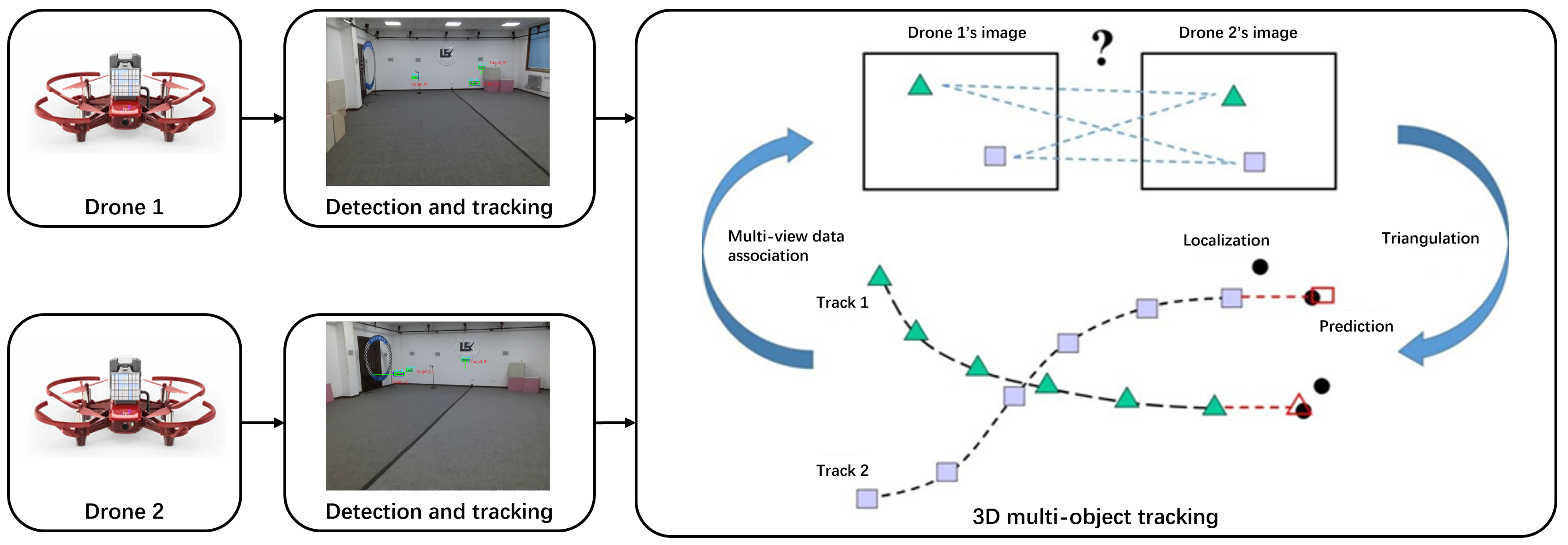
In multi-drone multi-object scenarios, the correct identity assignment must be made before passive localization results. Because two crossing bearings are sufficient to “create” an object (see Figure 1), multiple cameras will inevitably generate numerous line-crossings in the presence of several objects, leading to mismatched pairs and false positive objects. This section describes how the problem is formalized, which fuses temporal and spatial cues to filter out false positive objects and achieve accurate multi-object tracking.

3.1. Multi-View Data Association

At time step t, let the first drone-mounted camera detect n targets, denoted as X = { x i } i = 1 n , and the second drone-mounted camera detects m targets, denoted as Y = { y j } j = 1 m . Based on visual consistency and geometry, a maximum of p min ( n , m ) valid target correspondences can be established between a pair of drones, forming a set Z t = { z k } k = 1 p .
ρ = { ρ i j { 0 , 1 } } is a binary association variable, where ρ i j = 1 indicates that detection x i from the first camera and y j from the second camera correspond to the same physical object. The goal is to maximize the following matching score:
X ^ = arg max X ^ X f ( X , Y ; ρ , l i k e l i h o o d )
subject to
i ρ i j 1 , ρ i j { 0 , 1 }
where l i k e l i h o o d = { l i k e l i h o o d i j } quantifies the appearance and spatial similarity between detection pairs across views.
The scoring function is defined as Equation (3),
f ( X , Y ) = i , j ρ i j · l i k e l i h o o d i j

3.2. Multi-Object Tracking

Assume that q object detections are available at frame t 1 , denoted as O t 1 = { o s } s = 1 q . The associated objects from the current frame are given by Z t = { z k } k = 1 P . To maintain consistent tracking identities over time, we define a binary variable η = { η k s { 0 , 1 } } , where η k s = 1 denotes that the current observation z k corresponds to the previous observation o s .
The temporal data association problem, i.e., object tracking, is then defined as Equation (4),
Z ^ t = arg max Z ^ t Z t g ( Z t , O t 1 ; η , s i m i l a r i t y )
subject to
k η k s 1 , η k s { 0 , 1 }
where s i m i l a r i t y = { s i m i l a r i t y k s } measures the appearance or motion similarity between temporal observations.

4. Proposed Method

The overall pipeline of the proposed method is illustrated in Figure 2. First, a 2D image object detector and tracker are employed to build a multi-view association likelihood matrix. Next, the spatial and temporal cues are fused to perform object identity assignment. The valid correspondences are then used for passive 3D localization of the objects. Finally, the localized objects initialize and update a Kalman filter, yielding robust 3D multi-object tracking considering the uncertainty of localization.

4.1. 2D Multi-Object Tracking

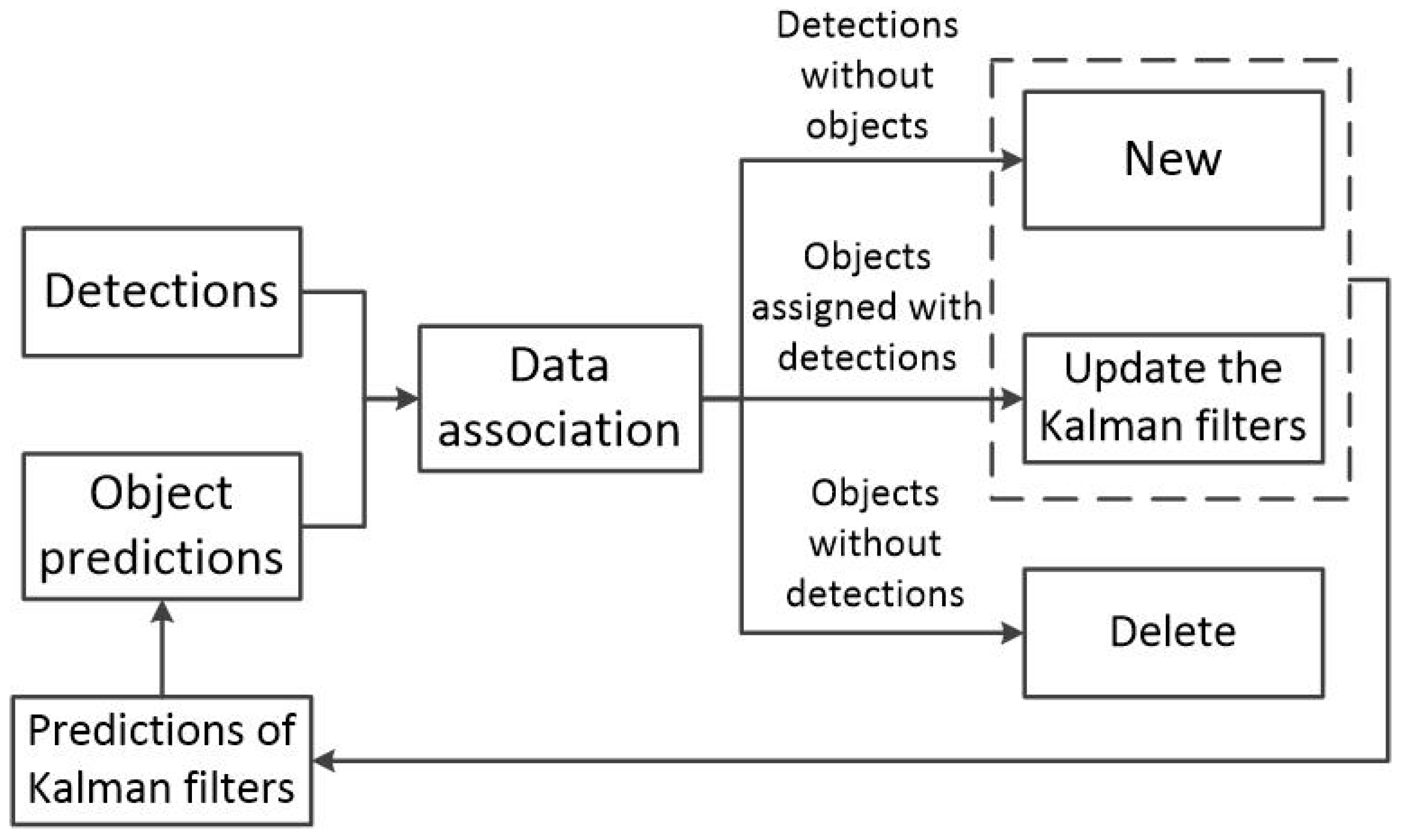
Reliable 2D multi-object tracking is crucial for subsequent multi-view data association. We employ a modified SORT tracker [10] on both observer drones, which replaces the Intersection over Union (IoU) metric with Euclidean distance to reduce sensitivity to camera ego-motion. The YOLOv8 [19] detector drives the process as shown in Figure 3: the Kalman filter predicts object states, a cost matrix between detections and predictions is solved by the Hungarian algorithm, and the resulting assignments update existing tracks, spawn new ones, or purge aged trajectories that exceed the lifetime limit.
A simple Constant Velocity (CV) motion model is implemented in the Kalman filter, with the process and observation noise covariance matrices initialized as diagonal matrices. The state vector and observation vector are defined as follows, respectively,
x 2 D = [ x c , y c , w , h , x ˙ c , y ˙ c , w ˙ , h ˙ ] T
z 2 D = [ x c , y c , w , h ] T
where x c , y c are the center pixel coordinates of an object’s tracking bounding box, and w , h are the width and height, respectively.

4.2. Multi-View Data Association

In multi-drone multi-object tracking, associating targets across different views is challenging due to the high appearance similarity and motion variability of the aerial objects. Although feature matching can establish correspondences by extracting and comparing key points with their descriptors, aerial objects are often small and visually similar, making decisions based on appearance highly unreliable. We therefore rely on spatial-motion evidence with temporal consistency to eliminate false positive objects, providing a robust solution to the multi-view data association problem. A two-stage object identity assignment method is proposed that leverages spatial consistency and temporal continuity.
At time step t, two observer drones detect targets, forming 2D bounding box sets D i t . These detections are tracked to produce trajectories T i . The center c i t , j of each bounding box is back-projected using camera intrinsics K i and extrinsics [ R i , t i ] into a bearing vector l i t , j . Given a bearing pair ( l 1 t , j , l 2 t , k ) , their closest 3D intersection x j k t is computed. Reprojecting x j k t into both views yields image points c ^ 1 t , j and c ^ 2 t , k . The reprojection error can be calculated as follows:
ϵ j k t = 1 2 c 1 t , j c ^ 1 t , j 2 + c 2 t , k c ^ 2 t , k 2
The spatial likelihood is then defined as Equation (9),
L j k spatial ( t ) = exp ( λ ϵ j k t )
where λ is a scaling factor that controls the sensitivity of the spatial likelihood to the reprojection error.
We found in real experiments that false positive objects do not jump randomly but rather exhibit continuous trajectories, much like actual targets. Moreover, at a certain instant, a false positive localization may even lie closer to the actual target position than the correct localization, as illustrated in Figure 4:
There are 9 localization hypotheses triangulated by bearing pairs, indicated by blue arrows, whereas green arrows show estimated tracks. Inside the red rectangle, the correct localization for the object i d = 3 is actually farther from the ground-truth position than the false positive localization. At this instant, the pair of bearings that produces the false positive localization yields a smaller reprojection error than the pair associated with the true target. Thus, the spatial cues do not always guarantee a valid localization. The geometric relationship between observers and observed objects also affects the reliability of multi-view association. When all observers and observed objects lie approximately in the same spatial plane, criteria relying solely on spatial cues become ineffective, making it impossible to distinguish true targets from false positive ones.
To incorporate temporal information, we define a history-based indicator, as Equation (10),
W j k t = l = t w t 1 δ j k l
where δ j k l = 1 if the pair ( j , k ) is matched at frame l, and 0 otherwise. w is the time window and is empirically determined based on experiments. The shorter history (e.g., time window of 2) is less effective at suppressing false positive localizations. A window size of 5, which performs similarly to 8, offers a suitable trade-off for our scenario.
The combined spatio-temporal likelihood becomes
L j k combined ( t ) = L j k spatial ( t ) · 1 + α · W j k t
We solve the optimal assignment using the Hungarian algorithm over L j k combined ( t ) , which yields a set of matched pairs that do not overlap. Each pair of matched bearings is triangulated to produce the 3D target set X t for further use in 3D object tracking.

4.3. 3D Multi-Object Tracking

3D multi-object tracking based on the Kalman filter consists of four main modules: state estimation, data association, state update, and track management. Two types of distance metrics, i.e., Euclidean distance and Mahalanobis distance, are integrated into the data association module to test and handle varying levels of noise and uncertainty, respectively.
The state vector x , observation vector z , process noise covariance matrix Q considering the noise source of camera motion, and observation noise covariance matrix R can be defined as follows:
x = [ x , x ˙ , y , y ˙ , z , z ˙ ] T
z = [ x , y , z ] T
Q = 1 2 Δ t 2 0 0 Δ t 0 0 0 1 2 Δ t 2 0 10 Δ t 0 0 0 1 2 Δ t 2 0 0 Δ t ( σ p y ) 2 0 0 0 ( σ p y ) 2 0 0 0 ( σ p y ) 2 1 2 Δ t 2 Δ t 0 0 0 0 0 0 1 2 Δ t 2 Δ t 0 0 0 0 0 0 1 2 Δ t 2 Δ t
R = diag ( σ o x ) 2 , ( σ o y ) 2 , ( σ o z ) 2
where x , y , z are the coordinates of the 3D position of the object. σ x , σ y , σ z represent the standard deviations of the errors in the x , y , z directions, respectively. Δ t is the time interval.
At each time step t, for each existing track, we predict the state of the object x j ( t ) based on a CV motion model. The prior estimation x ^ j ( t | t 1 ) is obtained via KF using previous states and process noise models. This results in a set of predicted target positions { x ^ j } j = 1 M , which serve as the basis for data association.
To associate the current 3D observations { z i } i = 1 N with predicted states, a similarity matrix is computed between observations and predictions. Euclidean distance and Mahalanobis distance are commonly used to represent similarity.
The Euclidean distance offers a simple and intuitive way to measure the similarity between a detection and a prediction. However, when objects are partially occluded or closely spaced, affinity scores based on Euclidean distance often lead to incorrect associations. In contrast, the Mahalanobis distance incorporates not only the geometric separation but also the detection uncertainty encoded in the observation noise covariance matrix.
The Euclidean distance between an observation and a prediction is calculated as
d Euc = z i x ^ j 2
This simple geometric metric is effective in scenarios with high measurement accuracy and spatially separated targets. A cost matrix is formed and optimized using the Hungarian algorithm to obtain the optimal matching.
To enhance robustness in dense or occluded scenes, we further incorporate the Mahalanobis distance. The error propagation process from the normalized plane to 3D space for a camera is first modeled, thereby constructing the observation error model. The following equation describes the back-projection process from the normalized plane of the camera to 3D space, where γ is the scale factor:
x w y w z w 1 = 1 γ K 1 x n y n 1 1 = a 11 a 12 a 13 a 14 a 21 a 22 a 23 a 24 a 31 a 32 a 33 a 34 a 41 a 42 a 43 a 44 z c x n z c y n z c 1
where x w , y w , z w are the 3D position coordinates of the object. x n , y n are the object’s position in the normalized plane of the camera, i.e., image coordinates divided by focal length of the camera.
Taking the differential of Equation (16) results in Equation (17),
d x w = a 11 z c d x n + a 12 z c d y n + ( a 11 x n + a 12 y n + a 13 ) d z c d y w = a 21 z c d x n + a 22 z c d y n + ( a 21 x n + a 22 y n + a 23 ) d z c d z w = a 31 z c d x n + a 32 z c d y n + ( a 31 x n + a 32 y n + a 33 ) d z c
The scale factor in the above equation γ = z c 1 can be obtained from the constraint equation shown below, while z w is determined through the dual-drone passive localization,
z w = z c · a 31 x n + a 32 y n + a 33 + a 34
z c = z w a 34 a 31 x n + a 32 y n + a 33
The above Equation (17) can be expressed in Jacobian matrix form as Equation (20),
d x w d y w d z w = a 11 z c a 12 z c a 11 x n + a 12 y n + a 13 a 21 z c a 22 z c a 21 x n + a 22 y n + a 23 a 31 z c a 32 z c a 31 x n + a 32 y n + a 33 d x n d y n d z c = J d x n d y n d z c
Assuming the Jacobian matrix J i models the propagation of observation errors from the normalized plane to 3D space for the camera i, of which the observation noise covariance R i is defined as follows:
R i = diag ( σ o i x ) 2 , ( σ o i y ) 2 , ( σ o i z ) 2
where σ o i x , σ o i y , σ o i z represent the standard deviations of the errors in the x , y , z directions.
Then, the observation noise covariance matrix for the target in 3D space is
R = J 1 R 1 ( J 1 ) T + J 2 R 2 ( J 2 ) T
Based on the carefully designed observation noise covariance matrix, the Mahalanobis distance d Mah between the observation z and the prediction vector x ^ is calculated as follows:
ϵ = z ( t ) H ( t ) x ^ ( t | t 1 )
S ( t ) = H ( t ) P ( t | t 1 ) H ( t ) T + R ( t )
d Mah = ϵ T S ( t ) 1 ϵ + ln | S |
where H is the observation matrix, and P is the estimation covariance matrix.
After successful data association, we perform state updates for the matched observations and predictions. To ensure consistent tracking while suppressing false positives, we apply the following lifespan threshold strategy:
  • A trajectory is terminated if it remains unmatched for more than T lost frames (set to 30).
  • A new trajectory is initialized only if a newly observed point is matched successfully for more than T init frames (set to 4). Otherwise, it is considered a false alarm and discarded.
This mechanism helps maintain stable tracking for valid targets while suppressing noisy or spurious detections.

5. Experiments

5.1. Experimental Settings

In this section, different conditions are considered: dynamic and static observation scenarios. Dynamic observation means that the observer drones are maneuvering to go forward and backward during experiments, and static observation implies that the observer drones are hovering in the air. We use the 3D MOT based on Euclidean distance with simple initialized Q and R matrices as the baseline method [9] to compare the proposed approach based on Mahalanobis distance with the designed Q and R matrices. Under both conditions, simulation and real-world experiments are conducted to evaluate the performance of our localization and tracking algorithms. HOTA [20], IDF1 [21], and MOTA [22] are adopted as the primary evaluation metrics for the multi-object tracking algorithms as follows:
  • HOTA provides a comprehensive assessment of algorithm performance by jointly measuring detection accuracy, data association quality, and localization precision, thereby balancing the algorithm’s effectiveness across multiple dimensions.
  • IDF1 evaluates the tracker’s ability to handle fragmented trajectories and reflects its stability in dealing with target loss and re-identification.
  • MOTA offers an overall assessment of both trajectory continuity and detector performance by quantifying the algorithm’s tracking effectiveness in terms of False Positives (FP), False Negatives (FN), and IDentity switches (IDsw). Specifically, FP denotes the number of times false alarms are incorrectly tracked as real targets, FN represents the number of true targets that are missed, and IDsw counts the occurrences of target identity changes during tracking.
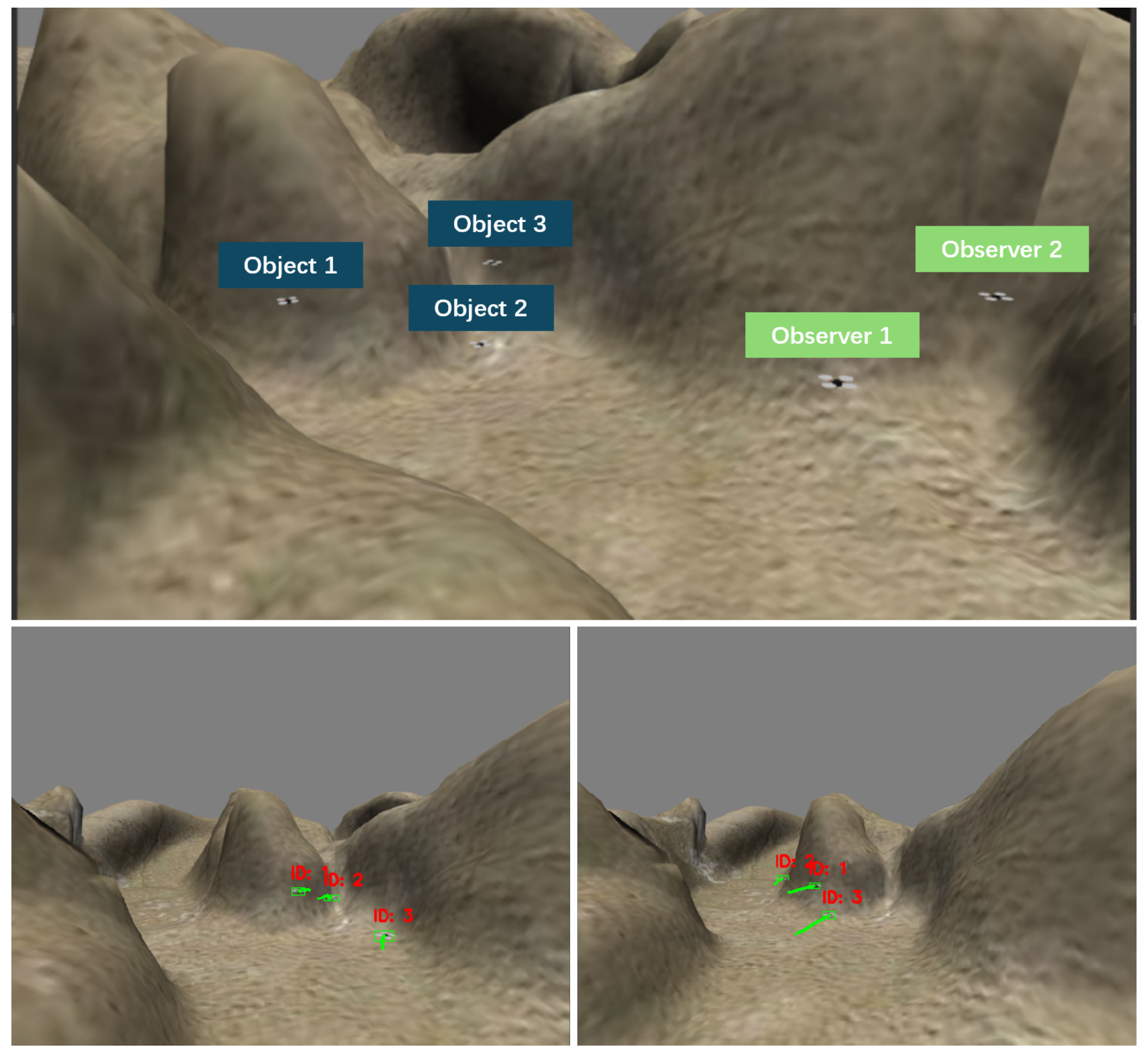
The simulation scenario is illustrated in Figure 5. It consists of 2 observer drones equipped with RGB cameras and 3 target drones with similar appearances. The camera resolution for all onboard sensors is 640 480 . The object detections from the two observation perspectives are shown in Figure 5.
The real-world experiments, which are illustrated in Figure 6, also consist of 2 observer drones and 3 objects. The camera resolution for all onboard sensors is 960 720 .
The motion capture system provides the ground truth positions of the objects and the 6D pose information of the observer drone. It is worth noting that, although we employ a motion capture system to determine the 6D poses of the observer drones, as well as the ground-truth positions of the target drones, the final triangulation-based localization requires the precise 6D poses of the observer drones’ cameras. This needs the calibration of the extrinsic parameters between the camera and the drone body. We estimated these extrinsic parameters using Apriltags [23]. However, this method remains coarse and is expected to introduce significant systematic errors. Errors in the cameras’ position and uncertainties in their angle introduce noise into the transformation process from 3D world coordinates to 2D image coordinates and ultimately distort the localization and association of the target across different viewpoints.

5.2. Experimental Results

5.2.1. Simulation Results

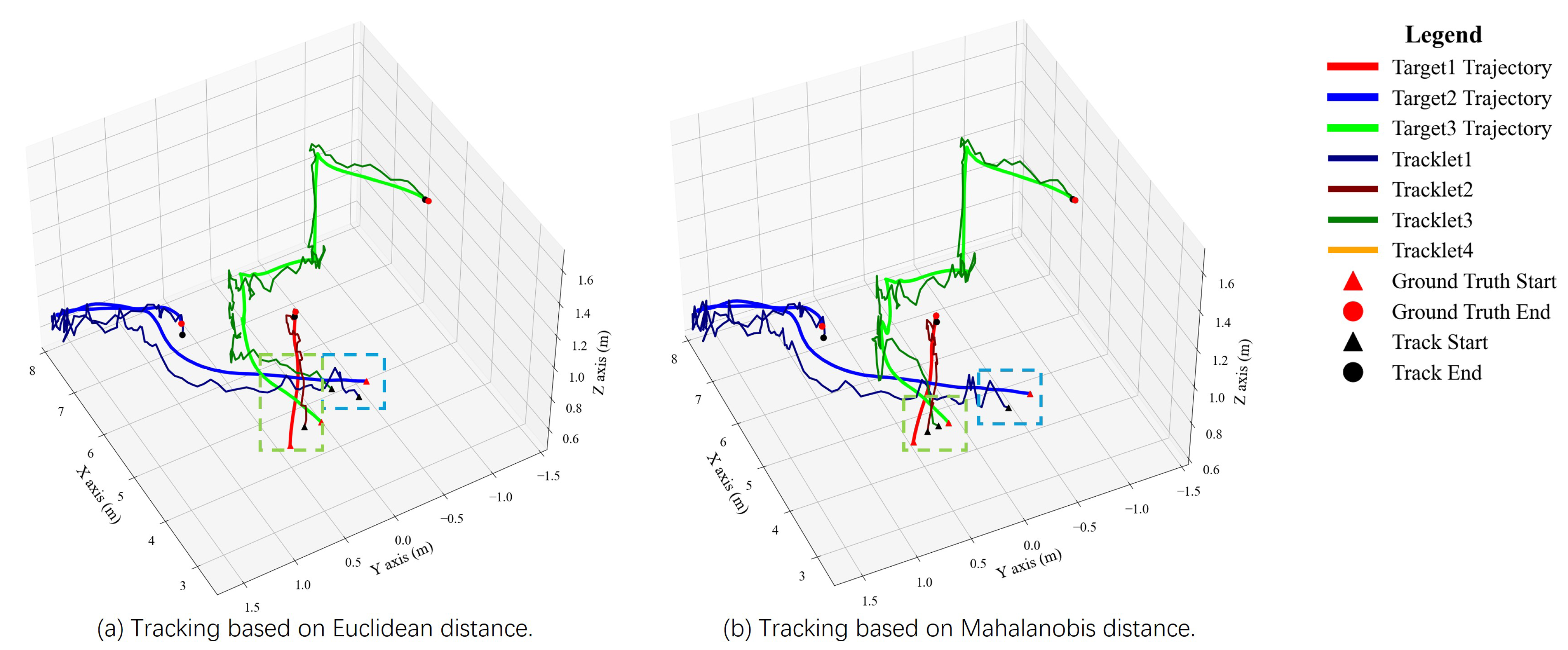
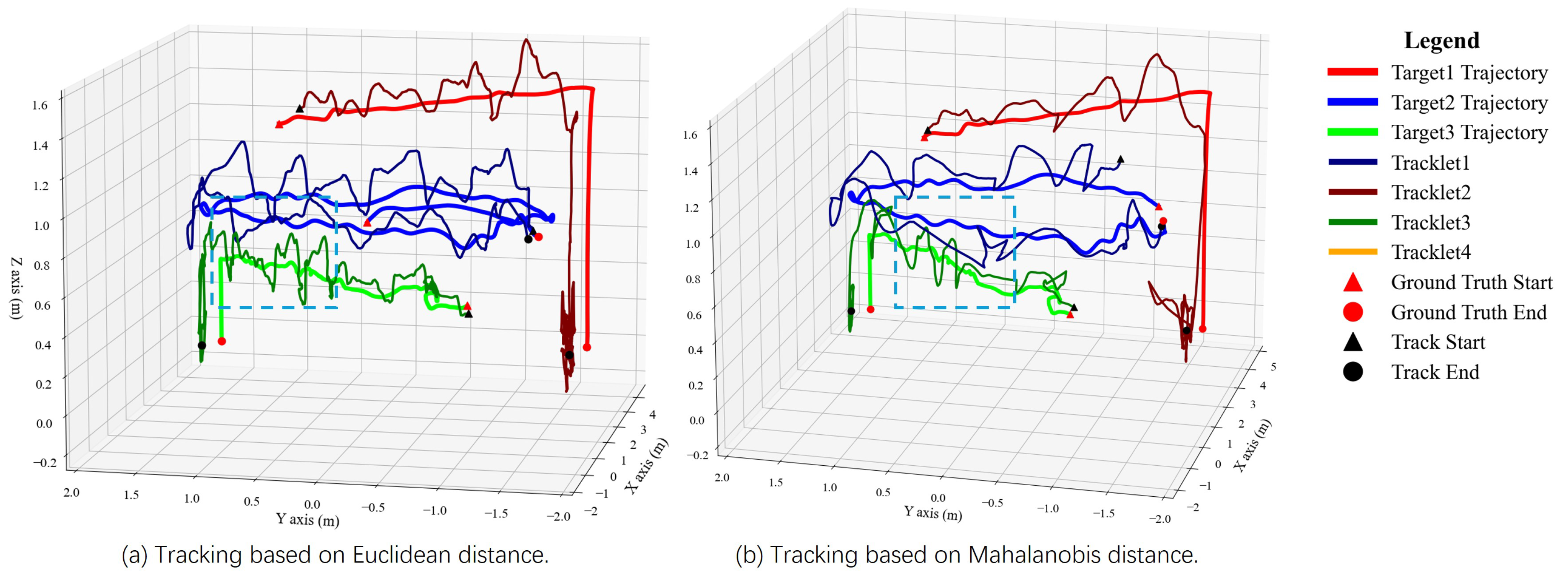
Under static observation conditions in the simulation, the tracking results based on Euclidean distance (i.e., the baseline) and Mahalanobis distance are shown on the left and right sides in Figure 7, respectively. The bold lines represent the ground-truth trajectories of the targets, while the thin lines denote the estimated tracking results. The triangle and circle indicate the starting and ending points of each trajectory, respectively. The coordinate axes are in m.
Both methods show some similar features of performance. There is a significant deviation in tracking object 3 (i.e., the green line) during the initial stage (highlighted by the green box). However, this deviation gradually decreases during subsequent localization and tracking. For object 1 (i.e., the red line), a noticeable deviation appears toward the end (highlighted by the red box), mainly due to missing object detection. Nevertheless, the Kalman filter can still provide effective prior state estimation, allowing the system to maintain a continuous target trajectory.
Compared with the baseline, our method benefits from considering localization uncertainty, which helps avoid mismatches during the data association process. As a result, the tracking deviation of object 3 in the initial stage is effectively reduced (as shown in the green box). In the late stage of tracking object 1, our method achieves higher tracking accuracy. However, trajectory fragmentation occurs (as shown in the red box) due to a temporary loss of localization information, which increases the observation noise and leads to data association failure.
As shown in Figure 8, under dynamic observation conditions, the baseline method experiences a noticeable decline in object localization accuracy due to the movement of the observer platform, which in turn reduces the stability of the tracking algorithm. In the final stage of tracking object 1 (as shown in the red box), the trajectory can still be roughly maintained. However, because the observation noise covariance is not carefully considered, the trajectory gradually diverges over time, leading to a significant decrease in tracking accuracy.
In contrast, when observation uncertainty increases significantly, the Mahalanobis distance-based tracking algorithm reinitializes new trajectories for tracking based on the latest target localization results. Although this process causes trajectory fragmentation, it effectively prevents error accumulation in the motion model and ensures higher accuracy during the initial stage of the new trajectory, thereby improving the overall tracking stability. A performance comparison between the baseline and our methods is presented in Table 1. An upward arrow means a higher value corresponds to better performance, whereas a downward arrow means a lower value reflects better performance. The best results are shown in bold.
The simulation evaluation results demonstrate that, under both static and dynamic observation conditions, our proposed method outperforms the baseline method across all performance metrics. Under static observation conditions, the MOTA and HOTA of our method are significantly improved, with a substantial reduction in FP and FN. The improvement of the IDF1 score and DetA indicates that the posterior prediction set of our method aligns with the true number of targets in space more frequently. The AssA increases by 25.4 , suggesting that the proposed method achieves a higher performance in data association between localized and predicted targets. Under dynamic observation conditions, the evaluation results are consistent with those obtained under static conditions, further validating the advantages and effectiveness of the proposed 3D MOT during the data association stage.
We further conducted ablation experiments on the two designed noise covariance matrices. Specifically, we performed simple initializations of the Q and R matrices separately (i.e., Ours-Q and Ours-R in Table 1), assigning only initial values to their diagonal elements. It can be observed that when using the simplified initialization strategies for Q and R matrices, there is no significant performance difference under static observation conditions. However, under dynamic conditions, the designed R matrix demonstrates a noticeable performance improvement. Moreover, the overall performance improvement of our approach is mainly from the reduction in FP and FN. The Mahalanobis distance with our derived R matrix creates an adaptive validation gate, while the baseline uses a rigid Euclidean threshold, accepting low-confidence localizations as valid tracks. In both static and dynamic scenes, Ours-R variant proves that without proper R matrix modeling, false positives surge even with our multi-view data association by spatio-temporal cues. The baseline suffers high FN because it loses tracks when observer drones move and noisy observations fall outside the association gate. Ours-R proves that our properly modeled Q matrix provides better motion priors to maintain track existence across observer drones moving and noisy observations to recover missing tracks.

5.2.2. Real-World Results

Under static observation conditions, the real-world experimental results are shown in Figure 9. For the baseline, the tracker initially fails to successfully track object 3, because the Euclidean distance-based data association erroneously linked the predicted state of object 3’s motion model to a false localization. As seen in Figure 9, this false localization is less than 1 m away from the true target position. Since the false localization also exhibited temporal continuity, its trajectory later intersects spatially with the true motion path of object 3, allowing the prediction to be correctly re-associated and thus correcting the previous association error.
In contrast, our method achieves correct data association for object 3 during the initial tracking phase, effectively avoiding false localization caused by intersection mismatches of bearings. Although occasional false localizations still influence the subsequent tracking, the algorithm can promptly correct such errors by accounting for observation uncertainty. Moreover, during the initial tracking of object 2, the Mahalanobis distance-based tracking effectively filters out false localizations during data association, resulting in a significantly reduced tracking error compared to the baseline.
As shown in Figure 10, under dynamic observation conditions, the localization error increases significantly, and tracking stability noticeably decreases. Nevertheless, our method successfully maintains consistent target identities throughout the entire experiment.
For the tracking of object 2, the baseline method exhibits state drift (as shown in the blue box), caused by incorrect data association. In contrast, our method effectively corrects the erroneous data association. At the final stage of object 1 tracking, both methods mistakenly associate the trajectory with false measurements, resulting in significant tracking errors.
The quantitative results are presented in Table 2. An upward arrow means a higher value corresponds to better performance, whereas a downward arrow means a lower value reflects better performance. The best results are shown in bold. Under static observation conditions, our method demonstrates superior overall performance. Under dynamic observation conditions, however, there is a slight decrease in MOTA ( 90.9 for Ours vs. 91.3 for Baseline) under dynamic real-world conditions. In real-world experiments, the motion of the observer drones introduces observation noise. This can lead to a higher number of False Negatives (FN), as some valid but noisy observations are correctly rejected as potential false positives rather than being incorrectly associated. This is reflected in the results (FN: 144 for Ours vs. 32 for Baseline), which is the primary factor for the slight MOTA decrease. However, it effectively suppresses False Positives (FP: 17 for Ours vs. 94 for Baseline), which is also reflected in Figure 11, indicating our method yields a more stable recall curve and maintains a relatively high recall level over a longer duration. Therefore, the results show a better performance of our method in identity preservation and false positive suppression, which are our key focus.
We further evaluate the performance of the proposed algorithm using the recall metric, defined as the ratio between the number of targets whose estimated positions are within a threshold distance (i.e., 1 m) to the ground truth and the total number of real objects present in the scene at that time.
The baseline exhibits a relatively low recall rate during the early stages of the experiment, indicating that some true targets are not successfully resolved at the initial phase. For our method, motion of the observer drones increases the uncertainty of localization results, which reduces the method’s sensitivity to discriminate true localizations from false ones.
In the real-world experiments, measurement uncertainty is noticeably larger. Under both static and dynamic observation conditions, simple diagonal initializations of the Q and R covariance matrices fail to produce satisfactory performance. These results corroborate the effectiveness of our carefully designed Q and R matrices.

6. Conclusions

In this work, we proposed a method focusing on multi-object tracking with distributed drones’ RGB cameras considering object localization uncertainty. With 2D image tracking and triangulation from different views, a likelihood association matrix, which integrated spatial and temporal cues, was employed to filter out false positive localizations effectively, enabling accurate multi-view data association. Subsequently, 3D multi-object tracking was implemented based on Mahalanobis distance with an observation noise covariance matrix characterizing the uncertainty of localization. Both simulation and real-world experiments validated the effectiveness of the proposed method. In the future, we plan to extend the proposed framework to larger multi-drone systems and investigate its robustness under more complex environments.

Author Contributions

Conceptualization, X.L. and T.Y.; methodology, X.L. and B.F.; software, B.F. and W.S.; validation, T.Y.; writing—original draft preparation, X.L. and B.F.; writing—review and editing, T.Y.; supervision, T.Y. and W.F.; project administration, T.Y. All authors have read and agreed to the published version of the manuscript.

Funding

This research was funded by the cooperative project between Shanghai Electro-Mechanical Engineering Institute and Northwestern Polytechnical University.

Data Availability Statement

The data presented in this study are openly available in https://github.com/npu-ius-lab/mdmot_bench, accessed on 31 December 2025.

Conflicts of Interest

Author Bohui Fang was employed by Xi’an Jingwei Sensing Technology Co., Ltd. The remaining authors declare that the research was conducted in the absence of any commercial or financial relationships that could be construed as a potential conflict of interest.

Abbreviations

The following abbreviations are used in this manuscript:
AOAAngle Of Arrival
MOTMulti-Object Tracking
KFKalman Filter
CVConstant Velocity

References

  1. Amosa, T.I.; Sebastian, P.; Izhar, L.I.; Ibrahim, O.; Ayinla, L.S.; Bahashwan, A.A.; Bala, A.; Samaila, Y.A. Multi-camera multi-object tracking: A review of current trends and future advances. Neurocomputing 2023, 552, 126558. [Google Scholar] [CrossRef]
  2. Yi, K.; Luo, K.; Luo, X.; Huang, J.; Wu, H.; Hu, R.; Hao, W. Ucmctrack: Multi-object tracking with uniform camera motion compensation. In Proceedings of the AAAI Conference on Artificial Intelligence, Vancouver, BC, Canada, 20–27 February 2024; Volume 38, pp. 6702–6710. [Google Scholar]
  3. Gunia, M.; Zinke, A.; Joram, N.; Ellinger, F. Analysis and design of a MuSiC-based angle of arrival positioning system. ACM Trans. Sens. Netw. 2023, 19, 1–41. [Google Scholar] [CrossRef]
  4. Chen, L.; Li, S. Passive TDOA location algorithm for eliminating location ambiguity. J. Beijing Univ. Aeronaut. Astronaut. 2005, 31, 89–93. [Google Scholar]
  5. Yu, H.; Wang, X.; Zheng, Z.; Peng, H. Formation maintenance strategy for USV fleets based on passive localization under communication constraints. Ocean Eng. 2025, 340, 122306. [Google Scholar] [CrossRef]
  6. Oualil, Y.; Faubel, F.; Klakow, D. A fast cumulative steered response power for multiple speaker detection and localization. In Proceedings of the 21st European Signal Processing Conference (EUSIPCO 2013), Marrakech, Morocco, 9–13 September 2013; IEEE: Piscataway, NJ, USA, 2013; pp. 1–5. [Google Scholar]
  7. Li, B.; Liu, N.; Wang, G.; Qi, L.; Dong, Y. Robust track-to-track association algorithm based on t-distribution mixture model. In Proceedings of the 2017 20th International Conference on Information Fusion (Fusion), Xi’an, China, 10–13 July 2017; IEEE: Piscataway, NJ, USA, 2017; pp. 1–6. [Google Scholar]
  8. Flood, G.; Elvander, F. Multi-source localization and data association for time-difference of arrival measurements. In Proceedings of the 2024 32nd European Signal Processing Conference (EUSIPCO), Lyon, France, 26–30 August 2024; IEEE: Piscataway, NJ, USA, 2024; pp. 111–115. [Google Scholar]
  9. Chen, G.; Fang, B.; Fu, W.; Yang, T. Multi-drone Multi-object Tracking with RGB Cameras Using Spatio-Temporal Cues. In Proceedings of the International Conference on Autonomous Unmanned Systems, Nanjing, China, 8–11 September 2023; Springer: Berlin/Heidelberg, Germany, 2023; pp. 412–421. [Google Scholar]
  10. Bewley, A.; Ge, Z.; Ott, L.; Ramos, F.; Upcroft, B. Simple online and realtime tracking. In Proceedings of the 2016 IEEE International Conference on Image Processing (ICIP), Phoenix, AZ, USA, 25–28 September 2016; IEEE: Piscataway, NJ, USA, 2016; pp. 3464–3468. [Google Scholar]
  11. Wojke, N.; Bewley, A.; Paulus, D. Simple online and realtime tracking with a deep association metric. In Proceedings of the 2017 IEEE International Conference on Image Processing (ICIP), Beijing, China, 17–20 September 2017; IEEE: Piscataway, NJ, USA, 2017; pp. 3645–3649. [Google Scholar]
  12. Zhang, Y.; Sun, P.; Jiang, Y.; Yu, D.; Weng, F.; Yuan, Z.; Luo, P.; Liu, W.; Wang, X. Bytetrack: Multi-object tracking by associating every detection box. In Proceedings of the European Conference on Computer Vision, Tel Aviv, Israel, 23–27 October 2022; Springer: Berlin/Heidelberg, Germany, 2022; pp. 1–21. [Google Scholar]
  13. Cao, J.; Pang, J.; Weng, X.; Khirodkar, R.; Kitani, K. Observation-centric sort: Rethinking sort for robust multi-object tracking. In Proceedings of the IEEE/CVF Conference on Computer Vision and Pattern Recognition, Vancouver, BC, Canada, 18–22 June 2023; pp. 9686–9696. [Google Scholar]
  14. Aharon, N.; Orfaig, R.; Bobrovsky, B.Z. BoT-SORT: Robust associations multi-pedestrian tracking. arXiv 2022, arXiv:2206.14651. [Google Scholar]
  15. Yang, M.; Han, G.; Yan, B.; Zhang, W.; Qi, J.; Lu, H.; Wang, D. Hybrid-sort: Weak cues matter for online multi-object tracking. In Proceedings of the AAAI Conference on Artificial Intelligence, Vancouver, BC, Canada, 20–27 February 2024; Volume 38, pp. 6504–6512. [Google Scholar]
  16. Pöschmann, J.; Pfeifer, T.; Protzel, P. Factor graph based 3d multi-object tracking in point clouds. In Proceedings of the 2020 IEEE/RSJ International Conference on Intelligent Robots and Systems (IROS), Las Vegas, NV, USA, 25–29 October 2020; IEEE: Piscataway, NJ, USA, 2020; pp. 10343–10350. [Google Scholar]
  17. Li, Y.; Guo, L.; Huang, X. Research and application of multi-target tracking based on GM-PHD filter. Opt. Photonics J. 2020, 10, 125. [Google Scholar] [CrossRef]
  18. Yin, T.; Zhou, X.; Krahenbuhl, P. Center-based 3d object detection and tracking. In Proceedings of the IEEE/CVF Conference on Computer Vision and Pattern Recognition, Nashville, TN, USA, 19–25 June 2021; pp. 11784–11793. [Google Scholar]
  19. Varghese, R.; Sambath, M. Yolov8: A novel object detection algorithm with enhanced performance and robustness. In Proceedings of the 2024 International Conference on Advances in Data Engineering and Intelligent Computing Systems (ADICS), Chennai, India, 18–19 April 2024; IEEE: Piscataway, NJ, USA, 2024; pp. 1–6. [Google Scholar]
  20. Luiten, J.; Osep, A.; Dendorfer, P.; Torr, P.; Geiger, A.; Leal-Taixé, L.; Leibe, B. Hota: A higher order metric for evaluating multi-object tracking. Int. J. Comput. Vis. 2021, 129, 548–578. [Google Scholar] [CrossRef] [PubMed]
  21. Ristani, E.; Solera, F.; Zou, R.; Cucchiara, R.; Tomasi, C. Performance measures and a data set for multi-target, multi-camera tracking. In Proceedings of the European Conference on Computer Vision, Amsterdam, The Netherlands, 11–14 October 2016; Springer: Berlin/Heidelberg, Germany, 2016; pp. 17–35. [Google Scholar]
  22. Bernardin, K.; Stiefelhagen, R. Evaluating multiple object tracking performance: The clear mot metrics. EURASIP J. Image Video Process. 2008, 2008, 246309. [Google Scholar] [CrossRef]
  23. Wang, J.; Olson, E. AprilTag 2: Efficient and robust fiducial detection. In Proceedings of the 2016 IEEE/RSJ International Conference on Intelligent Robots and Systems (IROS), Daejeon, Republic of Korea, 9–14 October 2016; IEEE: Piscataway, NJ, USA, 2016; pp. 4193–4198. [Google Scholar]
Figure 1. Distributed passive sensing needs to filter out false positive objects and achieve accurate multi-object localization and tracking.
Drones 09 00867 g001
Figure 2. The pipeline of the proposed system.
Drones 09 00867 g002
Figure 3. Multi-object tracking with Kalman filters.
Drones 09 00867 g003
Figure 4. A false positive localization may even lie closer to the actual target position than the correct localization.
Drones 09 00867 g004
Figure 5. Simulation settings.
Drones 09 00867 g005
Figure 6. Real-world experiment settings.
Drones 09 00867 g006
Figure 7. 3D MOT under static observation conditions in the simulation.
Drones 09 00867 g007
Figure 8. 3D MOT under dynamic observation conditions in the simulation.
Drones 09 00867 g008
Figure 9. 3D MOT under static observation conditions in the real-world experiments.
Drones 09 00867 g009
Figure 10. 3D MOT under dynamic observation conditions in the real-world experiments.
Drones 09 00867 g010
Figure 11. Recall based on Euclidean distance and Mahalanobis distance.
Drones 09 00867 g011
Table 1. Comparison of 3D MOT results in simulation experiments.
MOTA ↑IDF1 ↑HOTA ↑FP ↓FN ↓IDsw ↓AssA ↑DetA ↑
Static observation conditions.
Baseline [9]80.770.370.0161109062.578.5
Ours-Q99.797.981.730182.281.5
Ours-R96.496.381.2453182.080.5
Ours99.697.889.304187.990.6
Dynamic observation conditions.
Baseline [9]79.659.655.5166132041.075.2
Ours-Q99.097.580.9014179.882.0
Ours-R56.666.458.461917458.658.3
Ours99.097.582.0014180.683.4
Table 2. Comparison of 3D MOT results in real-world experiments.
MOTA ↑IDF1 ↑HOTA ↑FP ↓FN ↓IDsw ↓AssA ↑DetA ↑
Static observation conditions.
Baseline [9]60.477.258.531152063.653.9
Ours-Q53.962.647.263144647.347.3
Ours-R0.454.940.6324130648.434
Ours66.981.062.617136068.157.5
Dynamic observation conditions.
Baseline [9]91.395.772.89432074.571.1
Ours-Q50.974.757.3409312352.862.3
Ours-R37.73834.86122921645.726.6
Ours90.99470.417144071.769.1
Disclaimer/Publisher’s Note: The statements, opinions and data contained in all publications are solely those of the individual author(s) and contributor(s) and not of MDPI and/or the editor(s). MDPI and/or the editor(s) disclaim responsibility for any injury to people or property resulting from any ideas, methods, instructions or products referred to in the content.