An Improved Hierarchical Framework for Adaptive UAV Trajectory Planning in Dynamic Target Tracking

Highlights

What are the main findings?

• A novel kinodynamic planning framework is proposed, which efficiently integrates ESDF-based obstacle awareness directly into the search process for tracking a dynamic target.
• The introduced environment-adaptive risk-weight mechanism dynamically adjusts the search step size, enhancing planning efficiency and range without additional computational cost.

What are the implications of the main findings?

• The proposed intent-free motion prediction method, relying solely on spatiotemporal dynamics, offers a lightweight and versatile solution for tracking targets with unknown intentions.
• The method’s validation on a fully autonomous quadcopter demonstrates its practical applicability for real-world dynamic scenarios requiring robust motion planning and obstacle avoidance.

Abstract

Planning trajectories for unmanned aerial vehicles (UAVs) actively tracking a moving target poses a significant challenge. This paper introduces a motion planning system utilizing UAVs to track a dynamic target actively. The system can handle complex tracking tasks, ensuring safety and dynamic feasibility. Initially, a front-end path search involves employing adaptive Kinodynamic path searching to identify the route. A heuristic approach is applied to determine an initial trajectory, considering the minimum time and control cost. Subsequently, we introduce the cost of combining optimization and use Euclidean Signed Distance Field (ESDF) gradient information to improve trajectory smoothness and dynamic feasibility. Simulation results confirm the consistent superiority of our proposed method over the Fast-Tracker algorithm, resulting in shorter tracking distance and flight time. Our method achieves smoother trajectories while preserving dynamic feasibility. A real-world single-UAV experiment further validates the effectiveness of our approach.

1. Introduction

Unmanned aerial vehicles (UAVs), known for their ease of deployment and versatility, have become indispensable tools in various military and civilian applications, including search and rescue missions, reconnaissance, and surveillance [1,2,3]. In drone technology, a crucial application involves monitoring complex environments and dynamic targets often characterized by uncertain intentions. Active tracking of moving targets presents a significant challenge in this domain. This challenge is further intensified when tracking occurs in cluttered and a priori unknown environments. Here, the UAV must simultaneously map its surroundings, predict the target’s motion, and plan a safe, kinodynamically feasible trajectory, all under severe computational constraints. The failure of any component in this chain can lead to mission failure, highlighting the need for a robust and integrated approach.

Tracking dynamic targets presents a complex challenge, constrained by limited onboard computation, UAV dynamics, and stringent safety requirements for obstacle avoidance [4,5,6]. This challenge is traditionally addressed within the framework of maneuvering target tracking. The prevailing approach in this field relies on multiple-model methods, which simultaneously employ a set of models (and corresponding filters) to cover the possible dynamic behaviors of a target, as comprehensively surveyed by Li and Jilkov [7].

Such filtering-based approaches form the core of many practical Electro-Optical Systems (EOSs) for UAVs, as demonstrated by Kim et al. [8], who implemented a Kalman filter for image tracking and real-time 3D target localization on a small UAV. Their work exemplifies the successful application of classic estimation theory and also highlights the inherent system complexity and computational burden associated with achieving high-quality imaging, tracking, and measurement under SWaP constraints. To circumvent the dependency on explicit dynamic models, an alternative paradigm formulates the problem as a reactive control task.

Vision-based systems, for instance, achieve autonomous tracking by using visual trackers like LCT (Long-Term Correlation Tracking) with pixel-level feedback [9,10,11], effectively bypassing the need for explicit state estimation via filtering. For instance, Kumar et al. [12] demonstrated the detection, localization, and tracking of spherical targets using only onboard sensors. The primary focus of these approaches is the visual tracking scheme and the design of UAV control laws. By leveraging specific tracking strategies, they can achieve real-time performance. A fundamental limitation of these methods, however, is their general lack of environmental perception, which prevents them from incorporating critical safety and dynamic feasibility constraints. Regarding target prediction methodologies, some approaches employ Kalman filters integrated with coarse-grained motion models to forecast future trajectories [13,14,15]; however, their reliability is often limited by model inaccuracies. To address this limitation, hybrid estimation methods, such as the Interacting Multiple Model (IMM) algorithm, have been developed to better handle target maneuverability and nonlinearities [16,17]. Alternatively, intent-free planning methods have been proposed that predict target motion through polynomial or Bézier curve regression [18,19]. A significant drawback of such methods is their susceptibility to the Runge phenomenon and catastrophic failure during boundary extrapolation.

To address these limitations, researchers use the hierarchical framework method to address these challenges [20,21]. Hierarchical motion planning involves an advanced geometric path planner for initial path generation and a low-level time parameterization scheme for trajectory optimization. The advanced geometric path planner identifies an obstacle-free path to satisfy primary geometric constraints. Subsequently, the low-level time parameterization method accounts for drone dynamics and generates a time-parameterized trajectory. Thus, the advanced geometric path planner, often called front-end path planning, complements the low-level time parameterization, known as back-end trajectory optimization [22,23]. For rotor-based unmanned aerial vehicles with non-trivial dynamics, generating trajectories directly in high-dimensional state space is time-consuming, whereas developing geometric paths and applying smoothing calculations is more efficient.

Although effective in meeting real-time demands, this decoupling often sacrifices global optimality. The separation of geometric and dynamic constraints can result in trajectories trapped in local minima, especially during local replanning with a non-zero initial state. This frequently manifests as suboptimal smoothness and inefficient maneuvering when facing sudden obstacles or evasive targets. For instance, when facing sudden obstacles or target maneuvers during the tracking process, the planned trajectory is constrained within a topologically equivalent class [18,24,25]. This constraint can result in entrapment within local minima, leading to suboptimal flight smoothness and safety. Chen et al. [18] address the challenging problem of tracking a moving target in cluttered environments using a quadrotor. Their initial proposal involves an online trajectory planning method that generates smooth, dynamically feasible, and collision-free polynomial trajectories that track a visually tracked moving target. Ding et al. [26] propose a real-time B-spline based kinodynamic (RBK) search algorithm, transforming a position-only shortest path search into an efficient kinodynamic search by leveraging B-spline parameterization properties. Meanwhile, Dmitri et al. [27] describe a practical path-planning algorithm for autonomous vehicles operating in unknown environments with online obstacle detection. However, both [25,26] suffer from significant time complexity due to the need for fine-grained search. This may lead to low computational efficiency, which is not conducive to rapid route planning for complex environments and drones.

Beyond these, a distinct line of research employs hierarchical learning and control frameworks, such as those using Safe Reinforcement Learning (SRL) from human demonstration [28] and Hierarchical SRL with prescribed performance bounds [29]. These methods excel in learning complex skills from demonstration and providing strong theoretical safety and stability guarantees, often via Lyapunov analysis. However, their reliance on extensive pre-training data, complex neural network computations, and precise environment models presents a fundamental challenge for resource-constrained UAVs tasked with real-time, onboard dynamic target tracking. The computational overhead and data dependency of these SRL-based approaches stand in contrast to the need for a lightweight, self-contained algorithm that requires no prior demonstrations or complex online policy learning.

Therefore, a comprehensive solution is required that not only maintains the efficiency of hierarchical planning but also bridges the gap between geometry and dynamics to achieve higher performance. Such a solution should deliver real-time computational efficiency, robustness to prediction uncertainties, strict dynamic feasibility, and tight perception-planning integration.

To this end, we propose a solution framework to adaptively navigate and plan paths for unmanned aerial vehicles tracking dynamic targets in unknown obstacle scenarios. The contributions of this article are summarized as follows, with comparisons to state-of-the-art methods such as Fast Tracker [19]:

(1)

A lightweight, intent-free method for motion prediction driven purely by spatiotemporal dynamics, departing from any form of fitting-based prediction (e.g., trajectory fitting in Fast Tracker) to avoid extrapolation inaccuracies.

(2)

An environment-adaptive risk-weight mechanism for direct step-size determination in ESDF fine-grained search, enabling more efficient and reactive planning compared to fixed-step approaches.

(3)

The proposed approach is validated through extensive simulations and subsequently implemented on a fully autonomous quadcopter system. Real-world experiments are conducted to evaluate its performance in dynamic scenarios requiring motion planning and obstacle avoidance.

Overall, trajectory planning efficiency is enhanced through a kinodynamic framework that integrates ESDF calculation directly into the search process. This method accounts for dynamic constraints and incorporates an adaptive risk-weight strategy, which reduces time complexity without extra computational cost, thereby extending the planner’s range and precision.

2. Framework Overview

In UAV perception, both LiDAR and cameras have proven effective for environmental sensing. However, LiDAR’s significant weight and power consumption present substantial drawbacks for small UAVs, where payload and energy are critically constrained. For instance, typical high-resolution LiDARs used in robotics (e.g., the Livox Mid-360 laser scanner from Livox Technology Co., Ltd., Shenzhen, China) can weigh over 250 g and consume 6 W or more [30], whereas a lightweight camera system (e.g., the Intel RealSense D435i from Intel Corporation, Santa Clara, CA, USA) often weighs less than 100 g and consumes under 3 W [22]. This stark contrast in Size, Weight, and Power (SWaP) underscores the distinct advantages of cameras, making them particularly suitable for vision-based UAV applications. Consequently, our work employs a depth camera as the primary sensor to address the challenging problem of autonomous mobile target tracking. This task finds critical applications in security surveillance, filmmaking, and wildlife monitoring [13,20], where the depth camera provides essential geometric information for robust 3D tracking and obstacle avoidance.

As illustrated in Figure 1, our system is specifically designed for tracking a dynamic target in complex, unknown environments. The core problem we address is formally defined as: given the UAV’s current state $x_0(t)$ and the estimated state of the target $x_{\mathrm{target}}(t)$, compute a trajectory $\varsigma (t)$ for the UAV that minimizes a cost function $J(\varsigma )$ while satisfying (i) the UAV’s kinematic and dynamic constraints and collision-free conditions $\varsigma (t)\cap 𝒪=\varnothing$, where the obstacle set $𝒪$ is constructed from the depth camera data; (ii) real-time replanning requirements to adapt to the target’s unpredictable motion. This formulation of the tracking problem, which fuses target estimates with depth-based obstacle mapping, aligns with and extends previous research on drone-based pursuit [5,20] and specifically builds upon studies published in the Drones journal concerning moving target tracking [10,11].

Figure 1 illustrates the software architecture of our vision-based quadrotor automatic navigation system. The suggested trajectory planning framework (highlighted in yellow) is a planning module that encompasses the Adaptive Kinodynamic path search and B-spline-based optimization method (AKBS). The hardware components (highlighted in orange) comprise the sensing hardware and the UAV with its actuator. The sensing hardware includes a depth camera and an IMU. The Euclidean Signed Distance Field (ESDF) [31] and the state estimation module (VINS Fusion) [2] offer low-frequency local maps and high-frequency pose estimation. Following the map update, the planning module will initiate the replanning strategy and a fixed-frequency trajectory prediction.

Our trajectory planning framework utilizes an adaptive kinodynamic path search to generate initial, collision-free trajectories efficiently. This approach is detailed in Section 4. Subsequently, a computationally efficient optimization step refines these trajectories by adjusting their control points to enhance smoothness and guarantee dynamic feasibility, as elaborated in Section 5. A geometric controller tracks the desired trajectories generated by the real-time replanning module during flight [32]. The resulting attitude and throttle commands are then transmitted to the PX4 flight controller to guide the aerial vehicle toward the dynamic target. The experimental setup and results are detailed in Section 6.

3. Intent-Free Target Trajectory Prediction

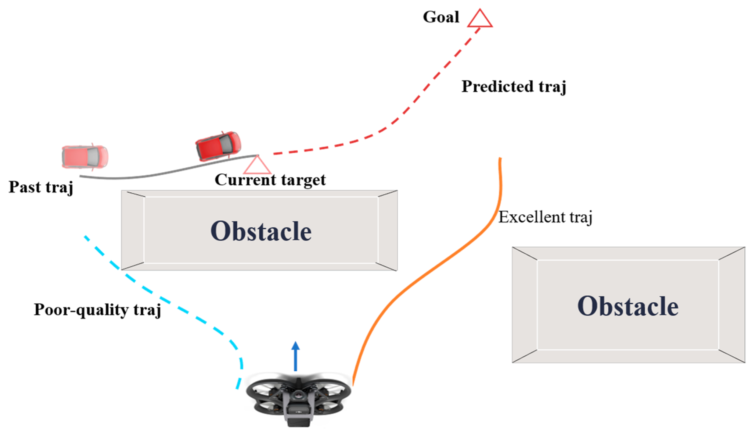
Trajectory prediction is essential for aerial drones to track moving targets, as conceptually illustrated in Figure 2. The figure contrasts two approaches: methods without prediction (red trajectories) can only react to the target’s current estimated position, resulting in inefficient, oscillatory paths that lag behind the target’s motion and greatly increase the risk of loss—a catastrophic failure in applications like surveillance. In contrast, our prediction-informed method (green trajectory) anticipates the target’s future motion. This enables the UAV to plan a smoother, more efficient path that proactively intercepts the predicted path, thereby minimizing tracking error. The surrounding obstacles, perceived by the depth camera, further define the feasible space for these trajectories, underscoring the necessity of prediction in complex environments. However, generating an optimal trajectory is challenging, especially for local replanning from a non-zero initial state, due to the target’s unknown intent and dynamic characteristics. Consequently, the planning module must perform high-frequency replanning. Longer prediction horizons generally lead to more globally optimal planning results, provided the predictions remain accurate.

Assuming the target’s current position ${\mathit{T}}_0\in {\mathit{R}}^2$ and velocity ${\dot{\mathit{T}}}_0\in {\mathit{R}}^2$ can be acquired via onboard sensors or communication, the objective is to predict its future position $\mathit{T}(t_p)$ at a fixed, known time horizon $t_p$. Algorithm 1 outlines the proposed intent-free trajectory prediction method for moving target. The proposed intent-free trajectory prediction algorithm is designed to address a critical challenge in vision-based UAV tracking: maintaining pursuit of a dynamic target in the absence of high-level intent information. In practical scenarios such as tracking a non-cooperative vehicle or a wild animal, the target’s ultimate goals and planned route are unknown to the UAV. Our algorithm operates under this key assumption, relying solely on real-time kinematic observations (position and velocity) from the onboard vision system. This makes it particularly suitable for applications like surveillance and filmmaking, where the target’s behavior is unpredictable, and the planner must react swiftly based on limited information. The core objective is to generate a short-term, kinematically feasible prediction to enable the UAV’s planner to proactively intercept the target, as opposed to lagging behind it.

Algorithm 1: Intent-free trajectory prediction algorithm for moving target
	Input: ${\mathit{T}}_0$, ${\dot{\mathit{T}}}_0$, $t_p$
	Output: Predicted trajectory $T^{*}$
1	$ini()$
2	$\mathit{T}(t_p)\leftarrow ComEnd()$
3	While $t<t_p$ do
4	for $\mathit{a}\in {\mathit{a}}_{list}$ do
5	$\mathit{x}(t+\Delta t)\leftarrow State(\mathit{a},\mathit{x}(t))$
6	end for
7	$T^{*}(t)\leftarrow Sort()$
8	Return $T^{*}$

Prior to the presentation of Algorithm 1, this section details the kinematic modeling of dynamic target. The model employs a second-order chain integral formulation, utilizing acceleration as the control input, as defined below (Note that the following formulation is independent of any knowledge regarding the target’s motion):

$$\begin{gathered} \dot{\mathit{x}}(\mathit{t})=\mathit{A}\mathit{x}(\mathit{t})+\mathit{B}\mathit{u}(\mathit{t}) \\ \mathit{A}=\left(\begin{array}{cc}{0}_{2\times 2}& {\mathit{I}}_2\\ 0_{2\times 2}& 0_{2\times 2}\end{array}\right),\mathit{B}=\left(\begin{array}{c}{0}_{2\times 2}\\ {\mathit{I}}_2\end{array}\right) \end{gathered}$$

(1)

The state vector $\mathit{x}(t)={\left(\begin{array}{cc}\mathit{T}(t)& \dot{\mathit{T}}(t)\end{array}\right)}^T$ encompasses the target’s kinematic properties, where $\mathit{T}(t)={\left(\begin{array}{cc}{\mathit{T}}_x(t)& {\mathit{T}}_{\mathrm{y}}(t)\end{array}\right)}^T$ denotes its 2D position, and $\dot{\mathit{T}}(t)$ represents its velocity. The control input $\mathit{u}(t)=\mathit{a}= \ddot{\mathit{T}}(t)$ is defined as the target’s acceleration, which drives the state evolution. The system matrix $\mathit{A}$ and the input matrix $\mathit{B}$ govern the internal dynamics and how the input affects the state, respectively. $\mathit{I}$ and $0$ represent the identity matrix and the zero matrix, respectively.

In Algorithm 1, $ComEnd()$ calculates a preliminary endpoint position $\mathit{T}(t_p)$ based on the target’s motion model:

$$\tilde{\mathit{T}}(t_p)={\mathit{T}}_0+{\dot{\mathit{T}}}_0\ast t_p$$

(2)

The position $\tilde{\mathit{T}}(t_p)$ serves as an estimate of the final state, providing the heuristic cost required to reach it. In line 4, ${\mathit{a}}_{list}$ denotes the discrete control input, defined as follows:

$${\mathit{a}}_{list}=\left\{-a_{\max },-{\displaystyle \frac{N-1}{N}}{a}_{\max },\dots ,{\displaystyle \frac{N-1}{N}}{a}_{\max },a_{\max }\right\},$$

(3)

In Line 6, the process $State()$ computes the target state $\mathit{x}(t+\Delta t)$ using Equation (1). This subsequent state is then used to select the optimal control input by applying a time-energy optimization principle:

$$\underset{\mathit{a}\in {\mathit{a}}_{list}}{\arg \min } f=g(\mathit{a})+h(\mathit{x}(t+\Delta t),\tilde{\mathit{T}}(t_p))$$

(4)

where $g$ denotes the actual cost, and $h$ denotes the heuristic cost.

$$\begin{array}{c}g(\mathit{a})={\lambda }_1‖\mathit{a}‖\\ h(\mathit{x}(t+\Delta t),\tilde{\mathit{T}}(t_p)=‖\mathit{T}(t+\Delta t)-\tilde{\mathit{T}}(t_p)‖\end{array}$$

(5)

The coefficient ${\lambda }_1$ balances the weight of these two cost components. Notably, Equation (5) employs the Euclidean distance from the target to the estimated position as a proxy for time. Once Equation (5) is computed, the optimal control input corresponding to the target position $\mathit{T}(t+\Delta t)$ is selected and appended to the predicted trajectory sequence ${\mathit{T}}^{*}$. This operation is executed in Line 7.

Compared to learning-based predictors [10], our method is data-efficient and does not require extensive offline training on specific motion datasets. It is robust to novel, unseen target behaviors since it is based on fundamental kinematics rather than pattern matching. However, a key limitation is its inability to leverage known contextual information or historical patterns for long-horizon prediction, which learning-based methods can potentially exploit if such data is available. Compared to other model-based predictors, such as the Constant Velocity (CV) or Constant Acceleration (CA) Kalman filters, our algorithm offers a significant advantage by explicitly generating and evaluating a set of kinematically feasible motion primitives. While a CV/CA model assumes a single, fixed motion model, our approach naturally encompasses a spectrum of maneuvers (e.g., sharp turns, deceleration) through the discrete control set ${\mathit{a}}_{list}$ making it more adaptable to agile targets.

The primary trade-off lies in computational cost. Simple filters like CV are computationally lighter, whereas our method involves online optimization over a control space, demanding greater processing power. This design choice is justified for our target tracking application, where prediction accuracy over a short horizon is paramount for collision-free interception. In summary, our predictor fills a niche between overly simplistic filters and data-hungry learning models, offering a principled, kinematics-driven approach for short-term prediction in unstructured environments.

4. Front-End: Adaptive Kinodynamic Path Searching

In dynamic target tracking, the trajectory planning module requires high-frequency replanning. Traditional methods, which generate trajectories based on the shortest path [33] (right curve, Figure 3), often result in dynamically infeasible and unsafe trajectories. This issue is particularly pronounced during local replanning with a non-zero initial state. In contrast, the proposed method produces a dynamically feasible and safe trajectory (left curve, Figure 3) by fully accounting for the aerial vehicle’s initial state and performing path searches informed by obstacle proximity. This work operates under the assumption that the target’s position is either perfectly perceived by the sensing algorithms or communicated to the UAV without obstruction.

Our kinodynamic search method builds upon a hybrid A* algorithm [18], expanding nodes (motion primitives) generated by discretizing the control input. This process identifies a safe and dynamically feasible trajectory within a voxel grid map. A key contribution is the thorough utilization of the ESDF map’s prior information to design adaptive search steps and pruning schemes, enabling an efficient, collision-free trajectory search. The complete front-end search process is outlined in Algorithm 2, where $O$ and $\mathbf{C}$ denote the open and closed sets, respectively. The open set is a priority queue that stores candidate nodes to be expanded, typically sorted by the sum of the cost from the start node and a heuristic estimate to the goal. The $\mathrm{findMinFCost}()$ operation selects the node with the lowest cost for expansion. The closed set records nodes that have already been visited and expanded to avoid redundant searches and prevent infinite loops. $\mathbf{Expand}\left(\right)$ implements the core node expansion process. It generates new candidate nodes by applying kinematically feasible motion primitives from the current node. The $\mathbf{contain}\left(\right)$ method (used as $\mathbf{C}.\mathbf{contain}\left(\right)$ and $\mathbf{O}.\mathbf{contain}\left(\right)$) checks whether a specific node is currently present in the open set or closed set, respectively. This is fundamental for the graph search logic to determine if a node is a new discovery, needs an update, or has already been processed. The $\mathbf{Occupy}\left(\right)$ function checks whether the node lies in an occupied space (collision check) using the ESDF. The algorithm maintains a parent-pointer for each node during the expansion phase (line 19: $n_i.parent\leftarrow n_c$), which records the optimal predecessor of the node. When the $\mathbf{NearEnd}()$ condition is met at node $n_c$, the Return Path() operation is invoked. This operation does not rely on a separately stored path variable. Instead, it dynamically reconstructs the optimal path by starting from the terminal node and sequentially tracing backwards through the chain of parent pointers until the start node is reached.

Algorithm 2: Adaptive Kinodynamic Path Searching
1:	Input: initial state ${\mathit{x}}_0$, goal state ${\mathit{x}}_T$
2:	Initialize()
3:	while $O$ is not empty do
4:	$n_c\leftarrow O.\mathrm{findMinFCost}()$, $O.\mathbf{pop}\left(\right)$
5:	if $\mathbf{NearEnd}(n_c)$ then
6:	Return Path()
7:	end if
8:	$nodes\leftarrow \mathbf{Expand}(n_c)$
9:	for  $n_i$ in $nodes$ do
10:	if $\mathbf{C}.\mathbf{contain}(n_i) \vee \mathbf{Occupy}(n_i)$ then
11:	continue;
12:	end
13:	$g_t\leftarrow n_i.g+\mathrm{EdgeCost}(n_i,n_c)$
14:	if $\neg \mathbf{O}.\mathbf{contain}(n_i)$ then
15:	$\mathbf{O}.\mathbf{insert}(n_i)$
16:	else if $g_t>n_i.g$ then
17:	continue;
18:	else if
19:	$n_i.g\leftarrow g_t$, $n_i.parent\leftarrow n_c$
20:	$n_i.f_c\leftarrow n_i.g+\mathbf{Heu}(n_i,x_T)$
21:	end if
22:	end for
23:	end while

Instead of straight lines, we use motion primitives respecting the aerial drone dynamic as graph edges. Motion primitives are represented by the struct node.

4.1. Motion Primitive

While the original Hybrid A* algorithm in [27] was designed for car-like robots in a 2D plane, our work constitutes a non-trivial extension to 3D space for quadrotor navigation, with key adaptations in state representation and motion primitives. The search state is defined as $x={[p_x,v_x,a_x,p_y,v_y,a_y,p_z,v_z,a_z]}^T$, and node expansion (Expand()) is governed by the UAV’s kinodynamic model presented in Equation (6) of this paper, which captures the full 3D translational dynamics—a fundamental departure from the 2D bicycle model in [27]. A critical enhancement for aerial navigation is the treatment of orientation: although yaw is not explicitly included in the kinodynamic search, the desired yaw angle $\phi$ for target tracking is geometrically derived from the generated path by aligning the UAV’s heading with the horizontal velocity vector $(v_x,v_y)$. Furthermore, leveraging the differential flatness property of UAV systems [34], the entire state and control inputs can be algebraically determined from the flat outputs $(x,y,z,\phi )$. Thus, the trajectory and yaw profile generated by our planner fully define the UAV’s motion, enabling accurate tracking by the downstream geometric controller [25]. We first discuss how to generate motion primitives in Expand(). Similarly to [34], using the differential flatness theory, the state of the aerial drone in path searching is represented by $x={[p_x,v_x,a_x,p_y,v_y,a_y,p_z,v_z,a_z]}^T$. With the third derivative of displacement $\mathit{j}=\stackrel{⃛}{\mathit{p}}$ as the control input $\mathit{u}$, the state transition equation is as follows:

$${\mathit{x}}_{k+1}=A{\mathit{x}}_k+B{\mathit{u}}_k,$$

(6)

$$A=\underset{i=1}{\overset{3}{\oplus }}\left(\begin{array}{ccc}1& \mathit{\tau }& {\displaystyle \frac{1}{2}}{\mathit{\tau }}^2\\ 0& 1& \mathit{\tau }\\ 0& 0& 1\end{array}\right) B=\underset{i=1}{\overset{3}{\oplus }}\left(\begin{array}{c}0\\ 0\\ 1\end{array}\right),$$

(7)

Here, the symbol $\oplus$ denotes the direct sum, which constructs the matrices $A$ and $B$ by stacking the enclosed matrix block diagonally three times, with all off-diagonal blocks being zero. $\mathit{\tau }$ is the expansion step, $u=[-u_{\max },u_{\max }]\in R^3$. In three-dimensional space, uniform discrete control inputs $\left\{-u_{\max },-{\displaystyle \frac{N-1}{N}}{u}_{\max },\dots ,{\displaystyle \frac{N-1}{N}}{u}_{\max },u_{\max }\right\}$. To fully leverage the prior information from the ESDF—a product of the mapping module that is reused by the planner without incurring additional computational cost—we introduce a risk weight parameter $\kappa$, defined as:

$$\kappa ={\displaystyle \frac{<\nabla d,v>}{‖\nabla d‖‖v‖}}-{\displaystyle \frac{90}{2\pi }},$$

(8)

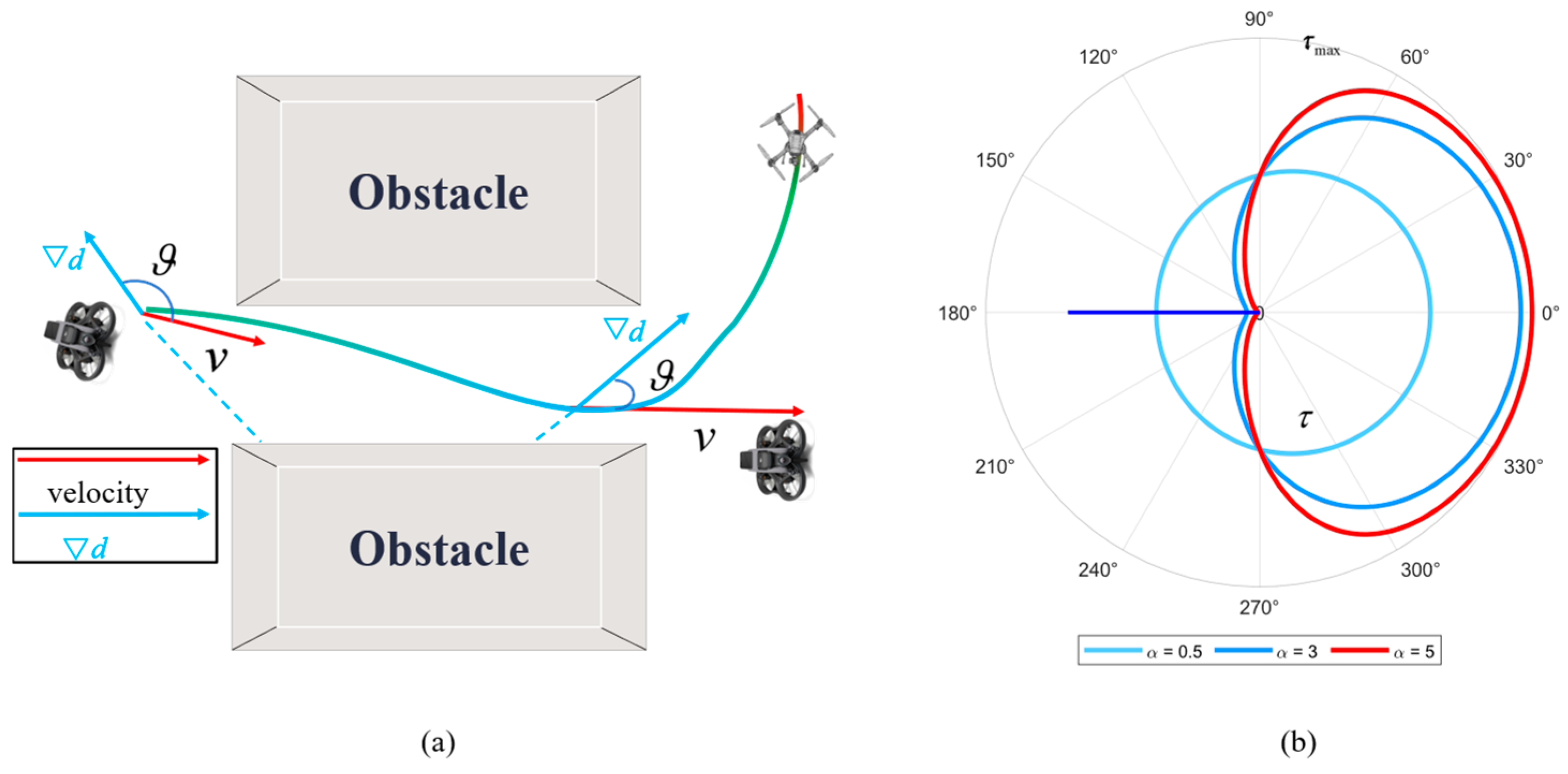
where $\nabla d$ is the gradient of the ESDF. As shown in Figure 4, when the velocity direction of the aerial drone is toward the obstacle, the gradient direction given by the ESDF is opposite to the velocity direction, which aggravates the maneuvering danger. Conversely, obstacle information can be disregarded when the gradient direction aligns with the velocity direction. The expansion step $\mathit{\tau }$ of the motion primitive is given by the following formula:

$$\tau (\kappa )=\min ({\displaystyle \frac{{\tau }_{\max }}{1+e^{\alpha \kappa }}},{\tau }_{\min }),$$

(9)

where $\alpha \in R^{+}$ is the rate-of-change coefficient. Evidently, the expansion step size is maximized when the directional angle is minimal. Conversely, the step size is minimized when the direction is opposed, as illustrated in Figure 4b.

Unlike traditional search-based path planning algorithms such as A*, which typically consider a fixed number of spatially adjacent nodes (e.g., 8 in 2D or 26 in 3D), the proposed algorithm incorporates a dynamically adjustable point expansion step size mechanism, as shown in Figure 5.

The non-uniform step expansion strategy differentiates our search algorithm and enhances aerial pathfinding in several key aspects. First, the well-designed mapping function in Equation (9) dynamically adjusts the expansion step size based on the risk weight $\kappa$, which is derived from obstacle proximity and velocity alignment. This mechanism ensures conservative steps near obstacles for safety while allowing larger steps in open spaces to enhance search efficiency, thereby preventing node expansion in hazardous proximity. Second, since computational time correlates with the number of expanded nodes, larger steps reduce the total node count, simultaneously promoting trajectories away from obstacles for improved safety. Third, compared to traditional A* [33], our method sparsely populates the search space, lowering computational load and enhancing real-time performance. Finally, the strategy fully incorporates the initial state during expansion, enabling dynamically feasible solutions for high-frequency replanning from non-zero initial states.

4.2. Actual Cost and Heuristic Cost

Following the terminology of A*, the cost of each node can be expressed as $f_c=g_c+h_c$. In this formula, $g_c$ denotes the actual cost from the initial state $x_0$ to the current state $x_c$, while $h_c$ represents the heuristic cost to search faster.

To achieve a trade-off between control-effort and trajectory duration, we minimize the cost function defined as:

$$J(T)={\displaystyle {\int }_0^T{‖u‖}^2}dt+\rho T,$$

(10)

In Algorithm 2, $\mathbf{EdgeCost}()$ calculates the cost of a motion primitive for each node extension, which is determined by the discrete control inputs and their duration. Under this formulation, the optimal search path is composed of a sequence of these motion primitives. Therefore, the cost function $g_c$ is defined as follows:

$$g_c={\displaystyle \sum _{i=1}^m{e}_i={\displaystyle \sum _{i=1}^m({‖u_i‖}^2+\mathit{\rho }}}){\mathit{\tau }}_i,$$

(11)

An admissible and informative heuristic is essential for accelerating the search process. To this end, the problem is formulated as a two-point boundary value problem [18,32]. Furthermore, the acceleration constraint is relaxed to reduce computational load.

$$\left[\begin{array}{l}{\alpha }_i\hfill \\ {\beta }_i\hfill \\ {\gamma }_i\hfill \end{array}\right]={\displaystyle \frac{1}{T^5}}\left[\begin{array}{cc}320& -120T\\ -200T& 72T^2\\ 40T^2& -12T^3\end{array}\right]\left[\begin{array}{l}\Delta p_i\hfill \\ \Delta v_i\hfill \end{array}\right],$$

(12)

Here, $\Delta p$ denotes the positional difference between the start and end points, and $\Delta v$ represents the velocity difference. $i$ represents three directions. Equation (12) incorporates the UAV’s initial velocity into the path search.

$\mathbf{Heu}()$ calculates this heuristic cost $J(T)$ by applying Pontryagin’s minimum principle to minimize the cost-to-go from the current state to the target state.

$$J(T)={\gamma }^2+\beta \gamma T+{\displaystyle \frac{1}{3}}{\beta }^2{T}^2+{\displaystyle \frac{1}{3}}\alpha \gamma T^2+{\displaystyle \frac{1}{4}}\alpha \beta T^3+{\displaystyle \frac{1}{20}}{\alpha }^2{T}^4,$$

(13)

So, $f_c=g_c+h_c={\displaystyle \sum _{i=1}^m({‖u_i‖}^2+\rho }){\tau }_i+J(T)$. Adjusting the expansion step size of motion primitives offers a tunable trade-off between path quality and computational completeness. Empirical results from both simulations and physical experiments validate the algorithm’s robust performance.

5. Back-End: Trajectory Optimization

While the proposed search algorithm efficiently generates an initial kinodynamically feasible path, the resulting path, like many sampling-based or graph-search methods, may still be in close proximity to obstacles due to the discrete nature of the search and the myopic nature of the cost function. This is a known limitation of such front-end path finders [35]. To address this issue and fully leverage the distance information in free space, we employ a B-spline-based trajectory optimization as the back-end. This two-stage strategy combines the robustness of the search algorithm in complex environments with the ability of gradient-based optimization to refine the trajectory for safety and smoothness. The key is to transform the sparse, discrete path waypoints from the front-end into a continuous, smooth, and collision-free trajectory that explicitly maintains a safe distance from obstacles.

5.1. Boundary Constraint

Boundary constraints define the fixed conditions for the initial state $x(t_0)$ and the final state $x(t_f)$ This work employs a B-spline for representing the UAV’s three-dimensional trajectory [36,37]. The core of our optimization is the formulation of a collision cost term that actively pushes the trajectory away from obstacles using the ESDF. As defined in Equation (20), this term penalizes control points where the distance to the nearest obstacle is below a safety threshold, ensuring the final optimized trajectory maintains a safe clearance.

The initial state of k degree B-spline is determined only by the initial k control points and the time interval. Given position constraint $\mathit{p}=[p_0,p_1,\dots ,p_{n-1}]$, the relationship between position and control points is defined as follows:

$$C_i={\displaystyle \frac{1}{6}}[p_i+4p_{i+1}+p_{i+2}],$$

(14)

Owing to the recursive property of B-splines, their derivatives are also B-splines. Consequently, the velocity and acceleration control points, denoted as ${\mathit{V}}_i$ and ${\mathit{A}}_i$, respectively, can be derived from Equation (13):

$${\mathit{V}}_i={\displaystyle \frac{C_{i+1}-C_i}{\Delta t}} , {\mathit{A}}_i={\displaystyle \frac{{\mathit{V}}_{i+1}-{\mathit{V}}_i}{\Delta t}},$$

(15)

where $\Delta t$ represents the knot span. For a uniform B-spline, the knot vector is defined such that the time difference between consecutive knots is constant. This time difference, denoted as $\Delta t$, is termed the knot span. Therefore, the boundary constraint of the aerial drone can be expressed by the following formula:

$$\begin{gathered} AC=B, \\ A={\displaystyle \frac{1}{6}}\left[\begin{array}{ccc}1& 4& 1\\ -3\Delta t& 0& 3\Delta t\\ 6\Delta t^2& -12\Delta t^2& 6\Delta t^2\end{array}\right], B=\left[\begin{array}{c}{p}_0\\ v_0\\ a_0\end{array}\right] or \left[\begin{array}{c}{p}_{end}\\ v_{end}\\ a_{end}\end{array}\right], \end{gathered}$$

(16)

where $C$ represent control points. The vectors $p_0,p_{end},v_0,v_{end},a_0,a_{end}$ represent the position, velocity, and acceleration at the trajectory’s start and end points, respectively. To accommodate high-frequency replanning, Equation (15) is applied iteratively throughout the process.

5.2. Trajectory Optimization

For a k-degree B-spline defined by n + 1 control points $\left\{C_0,C_1,\dots ,C_n\right\}$, boundary constraints fix the positions of the first and last k control points. Therefore, we optimize the remaining n + 1 − 2k control points and define the total cost function as follows:

$$J_{all}={\omega }_s{J}_s(•)+{\omega }_c{J}_c(•)+{\omega }_d{J}_d(•),$$

(17)

The total cost function includes smoothness cost ($J_s$), collision cost ($J_c$), and dynamic cost ($J_d$). ${\omega }_s$, ${\omega }_c$, and ${\omega }_d$ represent a trade-off between smoothness, safety, and dynamic feasibility.

In the context of 3D motion planning for UAVs, the dynamic constraints and operational requirements for vertical motion often differ from those in the horizontal plane. For instance, the acceleration and jerk limits along the z-axis are typically more conservative due to the need to directly counteract gravity and ensure stable ascent/descent. To accommodate these distinct characteristics and to enable independent control over the agility in the horizontal plane and the stability in the vertical direction, we formulate separate smoothness cost terms for the xy-plane and the z-axis.

The smoothness cost $J_s$ is defined using the squared norm of higher-order derivatives of the trajectory segments. To independently regulate the smoothness in the horizontal plane and the vertical axis, as motivated above, we decompose the cost into two orthogonal components using projection matrices. Let ${\mathit{T}}_{xy}=diag(1,1,0)$ and ${\mathit{T}}_{xy}=diag(1,1,0)$ be the projection matrices that extract the horizontal (x, y) and vertical (z) components from a 3D vector, respectively. The smoothness cost is then formulated as:

$$J_s={\displaystyle \sum _{i=1}^{n-k+2}{\omega }_{xy}{‖{\mathit{T}}_{xy}{\mathit{A}}_i‖}_2^2}+{\displaystyle \sum _{i=1}^{n-k+2}{\omega }_z{‖{\mathit{T}}_z{\mathit{A}}_i‖}_2^2},$$

(18)

where ${\omega }_{xy}$ and ${\omega }_z$ are their respective weighting coefficients. This formulation allows for fine-grained tuning; for example, a larger ${\omega }_z$ can be set to enforce a smoother, more conservative vertical profile, while a smaller ${\omega }_{xy}$ permits more aggressive maneuvers in the horizontal plane.

Noting the particular property of the B-spline, we convert the higher-order derivative information into the geometry information of the trajectory. So we rewrite $J_s$:

$$\begin{array}{ll}{J}_s=& {\displaystyle \sum _{i=1}^{n-k+2}{\omega }_{xy}{‖{\mathit{T}}_{xy}(C_{i+2}^{xy}-2C_{i+1}^{xy}+C_i^{xy})‖}_2^2}\\ & +{\displaystyle \sum _{i=1}^{n-k+2}{\omega }_z{‖{\mathit{T}}_z(C_{i+2}^z-2C_{i+1}^z+C_i^z)‖}_2^2}\end{array},$$

(19)

While the two formulations are fundamentally equivalent, Equation (18) offers distinct advantages: it relies solely on the trajectory’s geometric information, independent of time allocation, and it directly relates the cost to the optimization variables.

For the collision cost $J_c$, it is expressed as the repulsive force of the obstacle acting on each control point:

$$\begin{array}{l}{J}_c={\displaystyle \sum _{i=k}^{n-k}{f}_c(d(C_i))}\\ f_c(C_i)=\left\{\begin{array}{cc}0\hfill & d(C_i)>d_{thr}\\ {(d(C_i)-d_{thr})}^2& d(C_i)\le d_{thr}\end{array}\right.\end{array},$$

(20)

Here, $d(C_i)$ represents the distance from the i-th control point to the nearest obstacle, obtained from the ESDF gradient map, and $d_{thr}$ is the safety distance threshold. A penalty is applied when $d(C_i)$ falls below $d_{thr}$.

Dynamic feasibility is enforced by constraining all velocity and acceleration control points [38]. Consequently, penalties are imposed on the maximum velocity and acceleration of the aerial vehicle, formulated as:

$$\begin{array}{l}{J}_d={\displaystyle \sum _{i=1}^{n-k}{\omega }_v{f}_d({\mathit{V}}_i)}+{\displaystyle \sum _{i=1}^{n-k-1}{\omega }_a{f}_d({\mathit{A}}_i)}\\ f_d(c_r{|}_{r=x,y,z})=\left\{\begin{array}{cc}{a}_1{c}_r^2+b_1{c}_r+c_1\hfill & \hfill (c_r\le -c_j)\\ {(-\lambda c_m-c_r)}^3\hfill & \hfill (-c_j<c_r\le -\lambda c_m)\\ 0\hfill & \hfill (-\lambda c_m\le c_r\le \lambda c_m)\\ {(c_r-\lambda c_m)}^3\hfill & \hfill (\lambda c_m<c_r<c_j)\\ a_2{c}_r^2+b_2{c}_r+c_2\hfill & \hfill (c_r\ge c_j)\end{array}\right.\end{array}$$

(21)

The function $f_d(c)$ is an even function that applies no penalty when the velocity or acceleration magnitude remains below a specified threshold. When the threshold is exceeded, a two-stage penalty is activated: a cubic term imposes a progressively increasing cost for exceeding the maximum allowable rate, while a quadratic term is added to ensure numerical stability and prevent unbounded growth.

5.3. Optimization Strategy

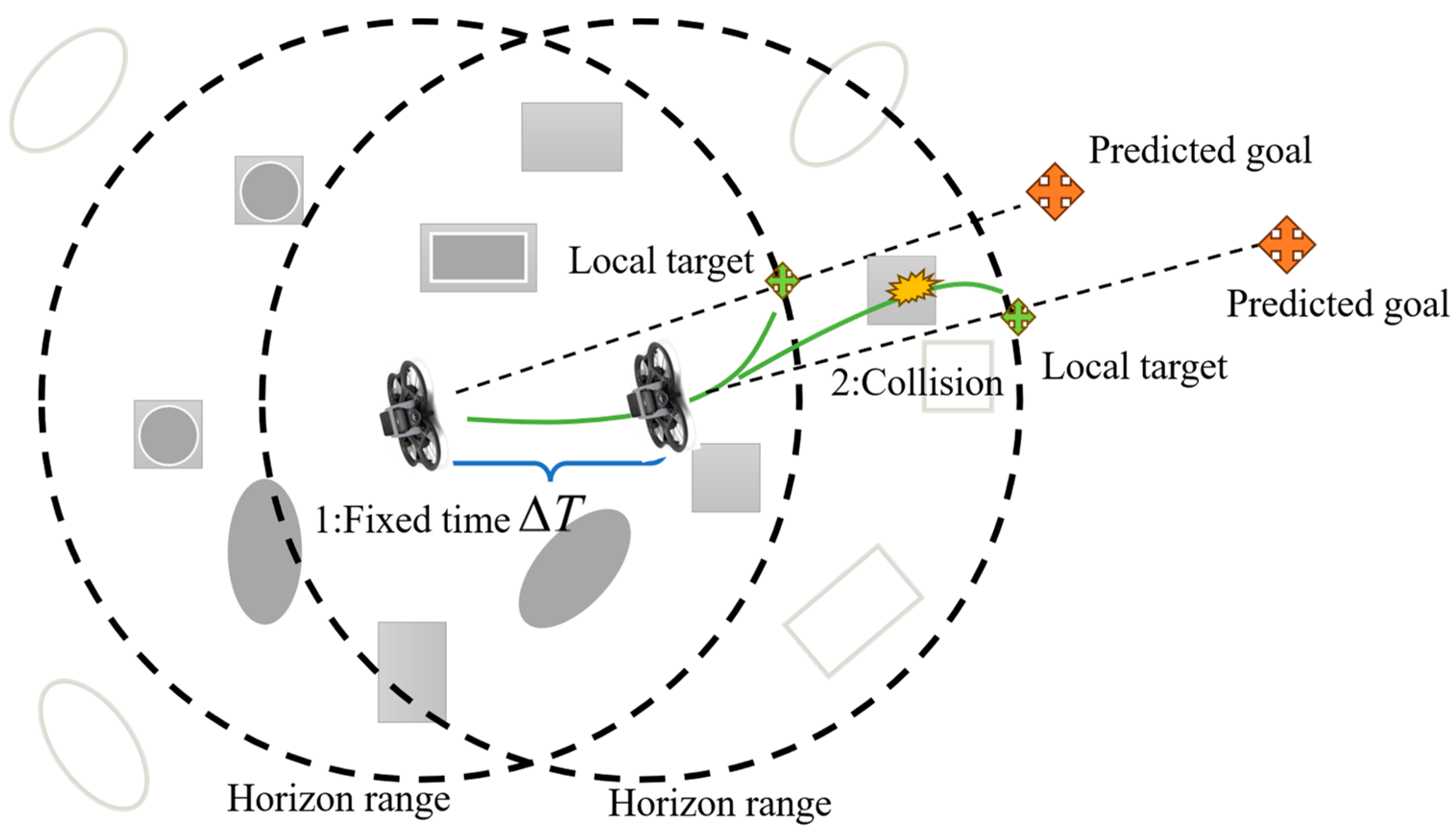
This local optimization strategy, also referred to as the Re-Planning Strategy, is illustrated in Figure 6. The process begins by establishing a global target using the prediction data from Algorithm 1. If this global target lies outside the horizon space (denoted by the dotted circle), a line is projected from the UAV’s current position to the global target. The local target is then defined as the point where this line intersects the horizon space boundary. Since planning outside this space is inefficient, all path search and trajectory optimization are confined within it.

Re-planning is triggered under two conditions, as shown in Figure 7. (1) Safety Check after Optimization: Our planning framework consists of a front-end path search that uses a discrete obstacle inflation for geometric feasibility, followed by a back-end trajectory optimization that employs soft constraints for smoothness and more precise obstacle avoidance. After the optimized trajectory is generated, a final safety validation is performed by discretizing the trajectory and rigorously checking for collisions against the ESDF. A re-planning cycle is immediately triggered if any discretized point on the optimized trajectory penetrates an obstacle (i.e., the signed distance ≤ 0). This ensures that the final output is strictly safe, even if the soft-constrained optimizer occasionally produces a trajectory that slightly cuts corners due to cost balancing. (2) Periodic Re-planning: The motion planning module is also invoked periodically at fixed time intervals of T = 0.5 s. This ensures system reactivity to new obstacles and dynamic changes that may not have been present during the previous planning cycle.

6. Result and Analysis

6.1. Implementation Details

The parameters of the proposed framework are summarized in

Table 1. Parametric setting for framework.

Module	Parameter	Description and Unit	Value
Environmental Perception and Map Representation	Resolution	Map resolution (m)	0.1
	ObsInflate	Obstacle inflate size (m)	0.099
Target Prediction	$t_p$	Predicted duration (s)	2
	${\lambda }_1$	Predicted coefficient	2
Path Searching	N	Number of Discrete Steps	3
	${\tau }_{\min }$	Minimum step constraint (s)	0.2
	${\tau }_{\max }$	Maximum step constraint (s)	0.8
	$\alpha$	change rate coefficient	3
	$\rho$	time penalty coefficient	10
Trajectory Optimization	Vmax	Velocity constraint (m/s)	2.5
	Amax	Acceleration constraint (m/s2)	3.5
	${\omega }_s$	Smoothness weight	1
	${\omega }_c$	Safety weight	0.5
	${\omega }_d$	dynamic weight	0.1
	${\omega }_{xy}$	horizontal (x, y) weight	1
	${\omega }_z$	Vertical plane weight	3
	$d_{thr}$	Safety threshold	0.4
	${\omega }_v$	Velocity weight	1
	${\omega }_a$	Acceleration weight	1
UAV parameters	m	Mass of UAV (kg)	2.5
	L	Wheelbase (mm)	410

. The grid resolution and obstacle inflation size were determined by considering the UAV’s physical dimensions and the available onboard computational resources. Specifically, the obstacle inflation size is set to 0.099 m to create a safety buffer around obstacles, effectively compensating for localization and control errors, which is critical for robust collision avoidance.

In the path searching module, the number of discrete steps $N$ significantly influences computational complexity, which grows exponentially with it. The time steps are not fixed but are allowed to adaptively vary between ${\tau }_{\min }=0.2$ s and ${\tau }_{\max }=0.8$ s, a range configured to thoroughly evaluate the UAV’s maximum flight speed and the trajectory tracking controller’s performance under dynamic constraints. The change-rate coefficient $\alpha$ was found to have negligible impact on performance within the range of 3 to 5, indicating a degree of algorithmic robustness to this parameter.

For trajectory optimization, the maximum velocity V_max and acceleration A_max constraints are dictated not only by the UAV’s physical limits but also by the experimental field size and safety considerations. The key weight coefficients—${\omega }_s$ (smoothness), ${\omega }_c$ (safety), and ${\omega }_d$ (dynamic)—were initialized based on values commonly adopted in related literature [38] and then fine-tuned through extensive simulation to balance flight agility against safety and smoothness. A sensitivity analysis revealed that the trajectory quality is most susceptible to the safety threshold $d_{thr}$ and the time-penalty coefficient $\rho$. An excessively small safety threshold increases collision risk, while an overly large one may render the optimization problem infeasible in cluttered spaces. Similarly, $\rho$ directly governs the trade-off between trajectory duration and smoothness.

Finally, the prediction horizon $t_p$ for target prediction is set to 2 s. This value represents a standard compromise; longer prediction periods lead to rapidly decaying accuracy due to increased uncertainty, while shorter horizons limit the system’s ability to react to target maneuvers.

The proposed motion planning method is implemented in C++14 and utilizes the lightweight L-BFGS nonlinear solver for optimization [39]. The target is modeled as a freely moving vehicle with a basic planning module. The mapping component of our framework integrates occupancy grid maps with ESDF. The occupancy map is maintained and updated following the methodology of FASTER [21], where the local map’s origin and data are refreshed based on odometry and depth images.

6.2. Simulation Result

We evaluated our AKBS-Tracker (Adaptive Kinodynamic path search and B-Spline-based optimization method) against the well-known Fast-Tracker system, a hierarchical framework for drone tracking, comparing trajectory smoothness, time, and tracking distance [15].

Trajectory Smoothness. A comparative analysis of planning results between AKBS-Tracker and Fast-Tracker under identical environmental conditions is presented in Figure 8. AKBS-Tracker generates shorter paths owing to its adaptive expansion step and demonstrates superior trajectory smoothness. This enhancement stems from the use of B-spline curves and a reduced number of path points in the back-end optimization, which inherently promotes smoothness. Additionally, the convex hull property of the B-spline contributes to safety. This property guarantees that the entire curve segment is strictly contained within the convex hull of its surrounding control points. Consequently, by ensuring that these convex hulls remain entirely within obstacle-free space, the trajectory itself is guaranteed to be collision-free. The resulting trajectory is not only visually smoother and more continuous but also improves the overall stability and reliability of the motion.

Time. To highlight the time advantage of AKBS-Tracker, the maximum speed of the Fast-tracker is set to 3 m/s. As shown in Figure 9, the performance of AKBS-Tracker and Fast-Tracker is compared in terms of speed and task completion time. Even when operating at a higher speed limit, Fast-Tracker required 13.49 s to complete the tracking task, which is 5.2% slower than the 12.78 s achieved by AKBS-Tracker, as shown in

Table 2. Flight times planned by different planners.

Tracker	Fast	AKBS	AKBS	AKBS	AKBS
	Time	Time	Average Time	Max Time	Min Time
flight time (s)	13.49	12.78	12.8387	13.07	12.74

. To ensure statistical significance, the experiment was repeated 10 times with different endpoints. AKBS-Tracker demonstrated consistent performance, with an average duration of 12.84 s and a maximum of 13.07 s.

Tracking distance. Figure 10 presents a comparison of tracking distance, where the proposed method consistently outperforms the Fast-Tracker planner. The red curve, representing the optimal case, achieves a maximum tracking distance of 3.03 m—merely 56.56% of the distance required by Fast-Tracker. Even the worst-performing case reaches only 85.82% of the competitor’s distance. This superior performance is attributed to the high-frequency replanning and the non-uniform expansion strategy of the front-end search algorithm. By incorporating the UAV’s initial velocity state, the algorithm facilitates faster convergence to the target point, while the non-uniform expansion significantly accelerates the search process.

To quantitatively assess the reliability and safety of the proposed planner, we conducted 30 simulation trials across a diverse set of scenarios with varying obstacle densities (ranging from 60 to 80 static obstacles) and target locations. The planner successfully generated and executed collision-free trajectories in 29 cases, resulting in a success rate of 96.7%. The relevant test results, including dataset, are available as per the Data Availability Statement.

A single planning failure occurred in the most cluttered scenario (80 obstacles). We analyzed this case to understand the system’s limitations. The front-end search successfully provided an optimal, collision-free initial path. However, the back-end optimizer failed to refine this path into a smooth, collision-free trajectory within the allocated time budget. The failure was attributed to the highly non-convex nature of the collision cost function in such a dense environment, which caused the gradient-based solver to become trapped in a poor local minimum. This highlights a known challenge for local optimization methods and represents a boundary of the current system’s performance.

6.3. Onboard Autonomous Flight

The experiment was conducted in an unknown indoor environment. The UAV platform, depicted in Figure 11, primarily comprises flight control hardware, an IMU, and a support frame. The onboard computing unit is an Intel NUC11-TNKi5, and the depth camera is a RealSense D435i.

The indoor motion planning task was performed in a cluttered environment, as illustrated in Figure 12. The UAV’s maximum velocity was constrained to 0.5 m/s to comply with the safety regulations of the testing facility.

The UAV’s flight is documented in Figure 13 and Figure 14. Figure 13 shows a grayscale image from the onboard camera, and Figure 14 provides a third-person view of the same flight. The experimental results confirm that the proposed algorithm achieves excellent real-time performance, running efficiently on the onboard microcomputer.

Figure 15 shows the UAV’s flight trajectory, demonstrating successful obstacle avoidance in an unknown environment and real-time tracking of local targets, which are the points where the line-of-sight to the global goal intersects the planning horizon (as defined in Section 5.3 and Figure 6). An initial discrepancy between the planned and actual trajectory is observed, which converges over time. This is attributed to the path search algorithm’s initial neglect of the yaw angle, causing a transient tracking error. Regarding velocity, Figure 16 confirms that the UAV’s speed remained within the predefined maximum limit, thus adhering to the specified constraint.

7. Conclusions

This paper introduced an integrated onboard motion planning framework for autonomous drones, with contributions in two key areas. First, we propose a lightweight, intent-free method for motion prediction driven purely by spatiotemporal dynamics, which provides a critical foundation for tracking unpredictable targets. Building upon this, a hierarchical planner combining front-end kinodynamic path searching and back-end B-spline trajectory optimization was developed to address the challenge of high-speed onboard replanning. The front-end search efficiently generates a safe, dynamically feasible initial path by incorporating a novel risk-weight parameter to reduce computational complexity. Subsequently, the back-end optimization refines this path for smoothness and safety using boundary constraints and gradient-based methods, leveraging the convex hull property of B-splines to enhance optimization efficiency. The proposed framework was rigorously validated through extensive simulations and real-world experiments, demonstrating robust performance. Our conclusions can be summarized as follows:

(1)

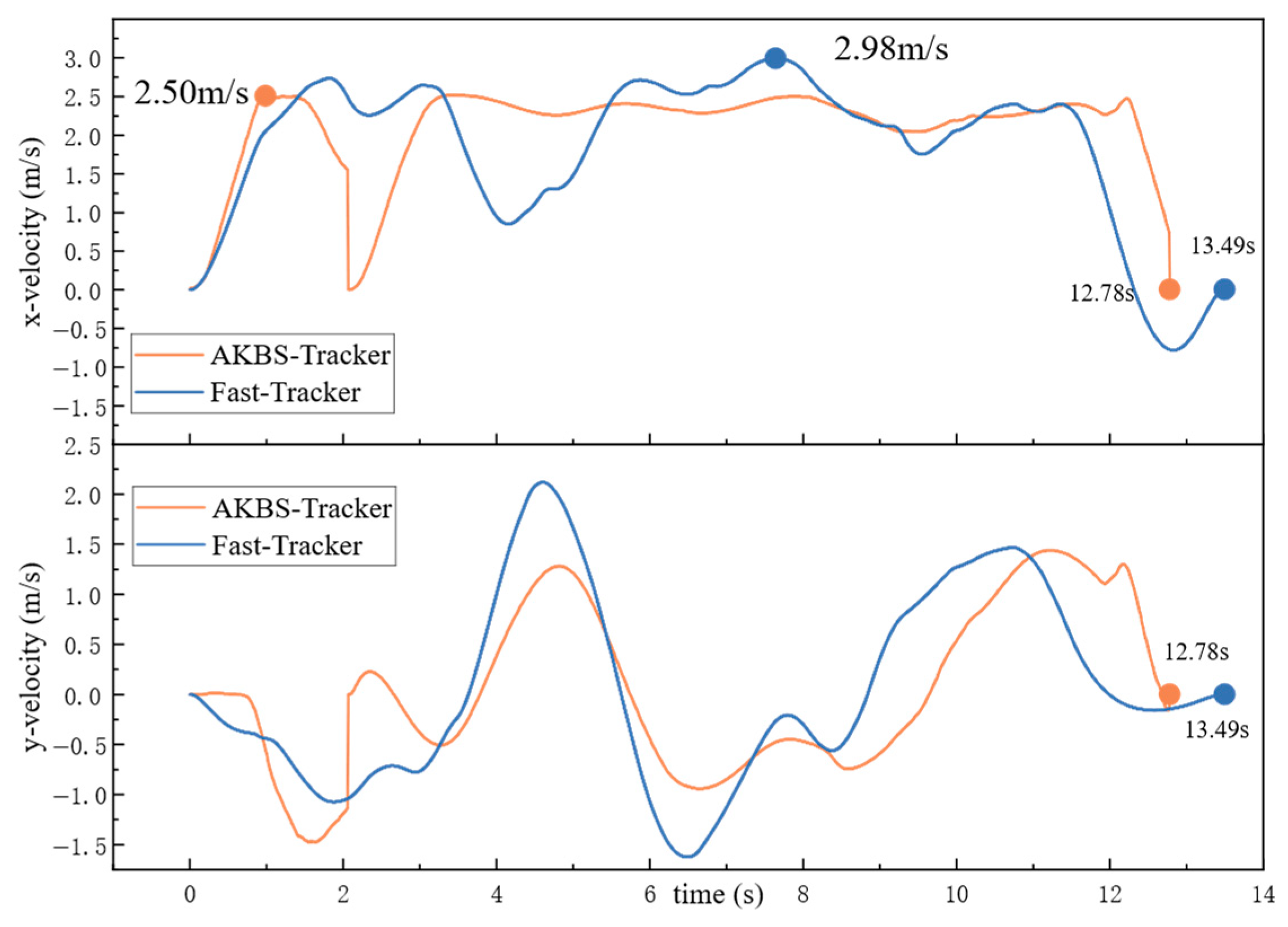
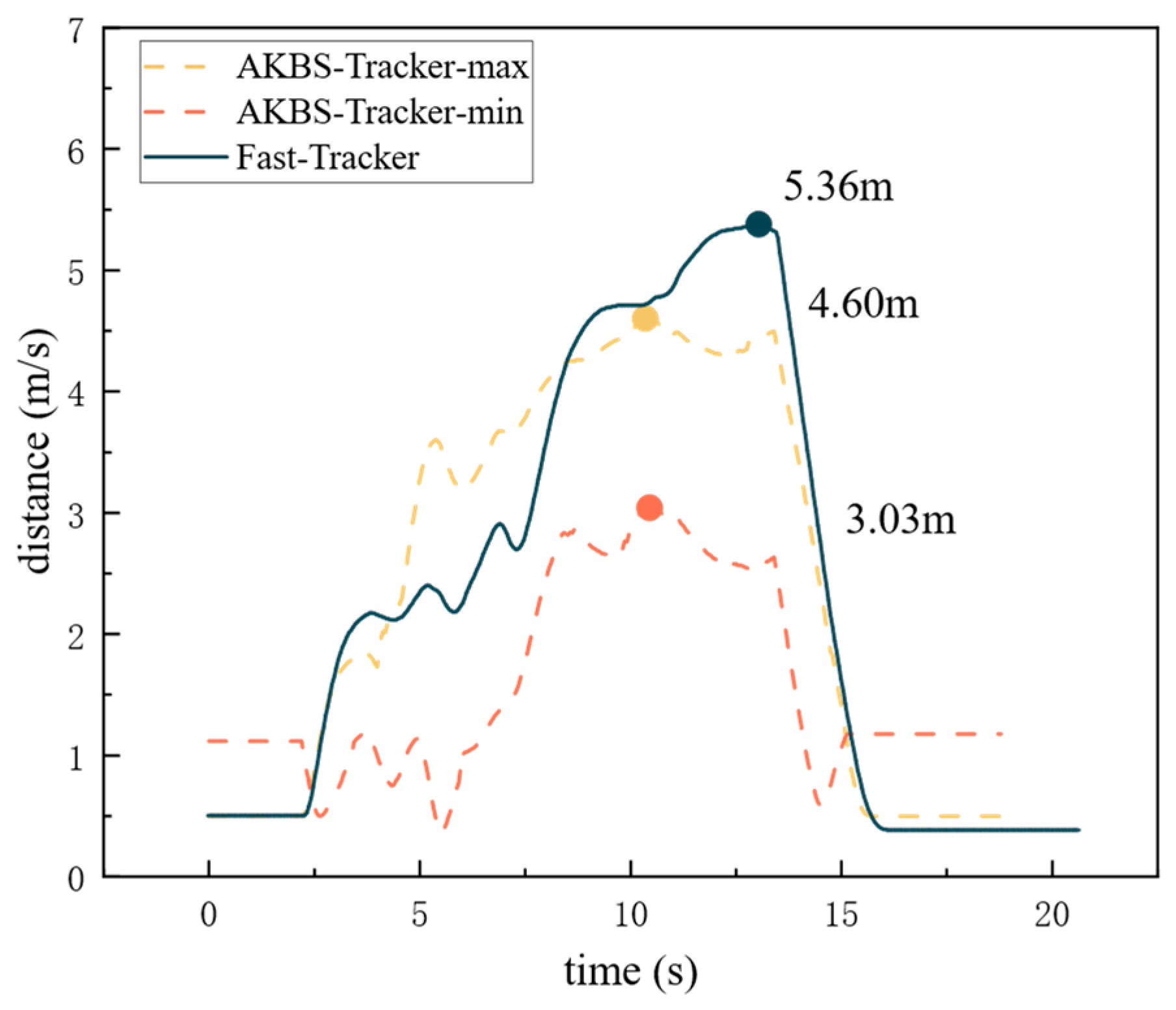
For trajectory planning for single drone target tracking, the proposed AKBS-Tracker generates shorter trajectories than the traditional Fast-Tracker, with notable advantages in trajectory smoothness, time and tracking distance.

(2)

The AKBS-Tracker decreased flight time effectively while maintaining the planned speed within the defined maximum speed limit, demonstrating its advantage in sustaining dynamic feasibility.

(3)

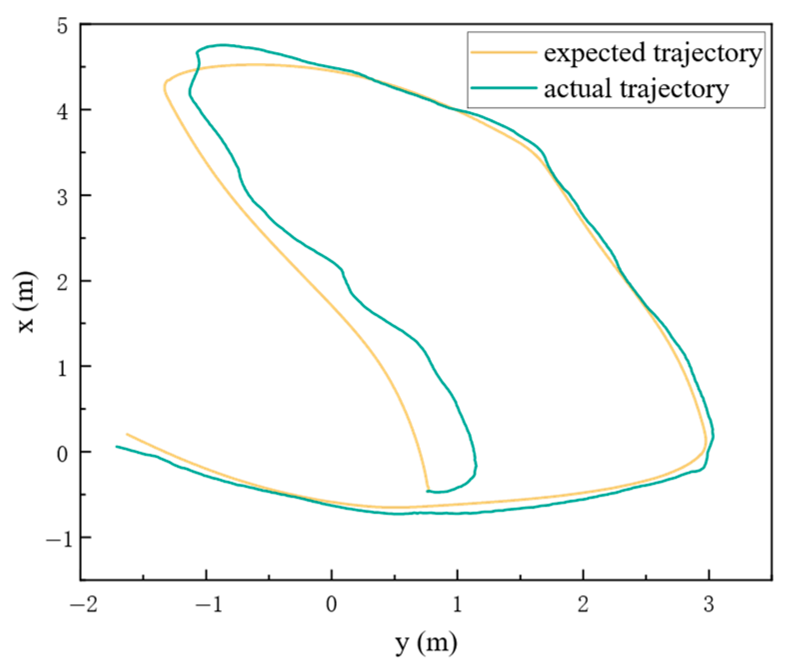
In a real-world experiment conducted in an unfamiliar indoor environment, the AKBS-Tracker successfully executed motion planning for a single UAV. It adeptly maintained a smooth and dynamic trajectory while skillfully avoiding collisions with obstacles. This experiment validates the system’s capability to operate safely and effectively in practical scenarios.

This research significantly improves autonomous UAV efficiency, safety, and practical applicability for target tracking. The potential impact extends to various applications, such as surveillance, delivery, and exploration. Nevertheless, acknowledging the limitations of our study is crucial. Given the limits of our study, we did not take into account the communications of tracking and visual occlusion. Subsequent research should take into account the robustness to sensor noise and communication delay. This can be achieved by scaling the approach, integrating advanced sensors, creating adaptive algorithms, conducting real-world experiments, and facilitating practical implementation in various applications.