Hybrid CFD-Deep Learning Approach for Urban Wind Flow Predictions and Risk-Aware UAV Path Planning

Highlights

What are the main findings?

• CFD-driven surrogate model combining a Convolutional Autoencoder (CAE) and a Deep Neural Network (DNN) enables rapid prediction of urban wind fields.
• Latent-space mapping efficiently encodes velocity and turbulence structures from RANS simulations with mean absolute errors below 1%.

What is the implication of the main finding?

• 4000× computational speed-up compared to CFD allows real-time deployment on embedded or edge hardware.
• Turbulence-aware UAV trajectory planning achieved via k-NANN graph discretization and A* search with TKE-based constraints.

Abstract

We present a CFD-driven surrogate modeling framework that integrates a Convolutional Autoencoder (CAE) with a Deep Neural Network (DNN) for the rapid prediction of urban wind environments and their subsequent use in UAV trajectory planning. A Reynolds-Averaged Navier–Stokes (RANS) CFD database is generated, parameterized by boundary-condition descriptors, to train the surrogate for velocity magnitude and turbulent kinetic energy (TKE). The CAE compresses horizontal flow fields into a low-dimensional latent space, providing an efficient representation of complex flow structures. The DNN establishes a mapping from input descriptors to the latent space, and flow reconstructions are obtained through the frozen decoder. Validation against CFD demonstrates that the surrogate captures velocity gradients and TKE distributions with mean absolute errors below 1% in most of the domain, while residual discrepancies remain confined to near-wall regions. The approach yields a computational speed-up of approximately 4000× relative to CFD, enabling deployment on embedded or edge hardware. For path planning, the domain is discretized as a k-Non-Aligned Nearest Neighbors (k-NANN) graph, and an A* search algorithm incorporates heading constraints and surrogate-based TKE thresholds. The integrated pipeline produces turbulence-aware, dynamically feasible trajectories, advancing the integration of high-fidelity flow predictions into urban air mobility decision frameworks.

1. Introduction

Urban Air Mobility (UAM) represents a transformative vision for city transportation, leveraging autonomous aerial systems like Unmanned Aerial Vehicles (UAVs) to alleviate ground congestion and enable novel services such as package delivery and infrastructure inspection [1,2]. Although the potential for UAM to revolutionize urban logistics is widely documented, its implementation faces significant technological and regulatory hurdles [3]. However, a critical challenge for its successful deployment is ensuring safe navigation through the complex urban airspace. This environment is dominated by dense building structures and intricate micrometeorological phenomena [4], which are often cited as a major weather-related hazard for low-altitude urban flights [5]. Among these phenomena, localized wind fields pose a particularly significant challenge. Therefore, accurate prediction of wind flow around buildings is crucial to ensure safety, reliability, and efficiency of UAV operations, particularly for trajectory planning and control systems operating in these dynamical environments [6].

The influence of urban wind on UAVs, especially on smaller platforms anticipated for UAM roles, is profound. These vehicles are highly susceptible to gusts and turbulent flows generated by buildings, which can severely impact stability, trajectory tracking, and energy consumption [6,7]. For instance, flight against headwinds has been shown to drastically increase power draw, thereby reducing the vehicle’s operational range and endurance [8]. Wind-induced deviations from planned routes and increased power requirements to counteract air currents can compromise mission objectives and endurance [9]. Furthermore, unexpected strong winds or turbulence can cause loss of control or collisions [10], highlighting the critical need for high-resolution wind information within UAV path planning algorithms to compute safe and dynamically feasible routes [11,12].

Computational Fluid Dynamics (CFD) offers a high-fidelity method for simulating these complex urban wind fields, capturing detailed three-dimensional flow patterns around obstacles [13]. Its use as a standard assessment tool is well-established in related fields like urban wind energy analysis [14], and is similarly fundamental to ensuring UAV operational safety. While accurate, CFD simulations are computationally intensive, often requiring hours (for steady-state atmospheric conditions) or days (for unsteady) on powerful hardware [15]. This computational burden makes direct CFD unsuitable for real-time applications like UAV path planning. This limitation has driven the development of surrogate models, which aim to emulate the behaviour of high-fidelity simulations at a fraction of the computational cost [16].

To overcome this challenge, data-driven modeling approaches have gained prominence. Techniques ranging from classical Proper Orthogonal Decomposition (POD) [17] to modern deep learning methods like Deep Neural Networks (DNNs) and AutoEncoders (AEs) offer pathways to create computationally efficient surrogate models that emulate CFD results with significantly reduced inference times [18,19]. Although there are various machine learning techniques, including probabilistic methods such as Bayesian Neural Networks that can quantify prediction uncertainty [20,21]—a valuable feature for risk-aware planning—this work focuses on developing a deterministic high-speed predictive model suitable for rapid deployment. The inherent complexity and high dimensionality of 3D flow fields necessitate powerful tools for information compression and relationship mapping. AEs, particularly convolutional variants, excel in extracting salient spatial features into a low-dimensional latent space, while DNNs can effectively learn the mapping from input parameters to this compressed representation [22,23].

In this article, we propose a data-driven framework to rapidly predict time-averaged urban wind fields for integration into UAV path planning systems. Our methodology involves first creating a database of high-fidelity CFD simulations where key atmospheric boundary conditions (e.g., inflow wind speed and direction) are parameterized. Each simulation yields a converged 3D wind field solution. This dataset, organized as a data tensor, is then used to train a deep learning model. Specifically, we employ a CAE to compress the high-dimensional wind field data into a low-dimensional embedding. A subsequent DNN is trained to predict this embedding directly from the input boundary condition parameters. This combined CAE-DNN architecture enables near-instantaneous prediction of the compressed wind field representation, which can then be rapidly reconstructed or used directly by path planning algorithms, circumventing the need for time-consuming CFD simulations during mission planning.

This paper details our approach and evaluates its performance. Section 2 describes the CFD setup and dataset generation. Section 3 outlines the CAE-DNN model architecture and presents results on prediction accuracy and computational speed-up. Section 4 discusses the model’s application in UAV path planning. Section 5 shows the principal results, while Section 6 provides conclusions and future work.

2. Numerical CFD Simulations

To develop a robust dataset of steady-state urban wind fields, high-fidelity simulations were conducted using OpenFOAM version 10 ( https://openfoam.org/version/10/), an open-source CFD software based on Finite Volume Method (FVM). As a case study, we employed the windAroundBuildings tutorial, a standard benchmark included in OpenFOAM distributions that simulates atmospheric boundary layer flow interacting with multiple building-like obstacles arranged in an urban layout. This makes it ideal for testing the sensitivity of wind fields to inlet conditions, building-induced turbulence, and recirculation zones, factors that critically affect UAV performance in UAM applications. These simulations provide ground-truth data for training and validating the data-driven surrogate models described later.

2.1. Computational Domain and Mesh

The CFD domain comprises a rectangular volume of [350 m, 280 m, 140 m], enclosing the building structures with ample space upstream and downstream to allow for flow development and wake resolution. A structured hexahedral mesh was generated using OpenFOAM’s blockMesh and refined near surfaces via snappyHexMesh. Local refinements were introduced around buildings to accurately capture shear layers and vortex shedding phenomena critical for downstream UAV trajectory planning. Finally, the mesh contained 385,166 cells (formed by 355,620 hexahedra, 25,806 polyhedra, and 3740 prisms), with a maximum non-orthogonality value of 45º and a minimum cell volume of 0.92. This mesh was selected after a sensitivity analysis, described in Section 2.2.2. 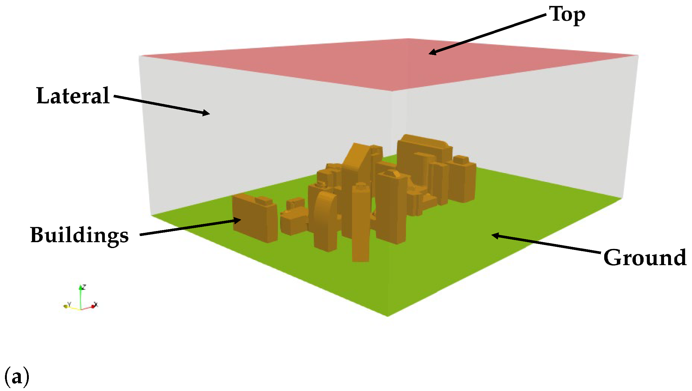Figure 1 shows the CFD domain with the different boundary surfaces and the mesh.

2.2. CFD Model

The steady-state Reynolds-Averaged Navier–Stokes (RANS) Equations (1) and (2) describe the averaged incompressible flow variables within the computational domain:

$$\nabla ·\langle \mathbf{u}\rangle =0$$

(1)

$${\rho }_{\infty }\langle \mathbf{u}\rangle ·\nabla \langle \mathbf{u}\rangle =-\nabla \langle p\rangle +\nabla ·[{\mu }_{\infty }(\nabla \langle \mathbf{u}\rangle +\nabla {\langle \mathbf{u}\rangle }^T)+{\overline{\overline{\mathbf{\tau }}}}^{Re}]$$

(2)

here, $\langle \mathbf{u}\rangle$ denotes the Reynolds-averaged air velocity, while ${\mu }_{\infty }$ is the constant dynamic viscosity of air (temperature-dependent viscosity variations and buoyancy effects were not considered in this study), set to $1.802·{10}^{-5}\mathrm{kg}/(\mathrm{m}\mathrm{s})$. The term $\langle p\rangle$ refers to the averaged pressure generated due to the flow motion, and ${\rho }_{\infty }$ is the air density, assumed constant and equal to $1.225{\mathrm{kg}/\mathrm{m}}^3$, due to the negligible impact of compressibility effects under the studied conditions.

To close the system of equations and model the Reynolds stress tensor in Equation (2), the standard $k-\epsilon$ turbulence model was employed, following the approach adopted in [16,24].

$${\mu }_t={\rho }_{\infty }{C}_{\mu }{\displaystyle \frac{k^2}{\epsilon }}$$

(3)

$${\rho }_{\infty }\langle \mathbf{u}\rangle ·\nabla k={\overline{\overline{\mathbf{\tau }}}}^{Re}:\nabla \langle \mathbf{u}\rangle -{\rho }_{\infty }\epsilon +\nabla ·\left(({\mu }_{\infty }+{\displaystyle \frac{{\mu }_t}{{\sigma }_k}})\nabla k\right)$$

(4)

$${\rho }_{\infty }\langle \mathbf{u}\rangle ·\nabla \epsilon =C_{{\epsilon }_1}{\displaystyle \frac{\epsilon }{k}}{\overline{\overline{\mathbf{\tau }}}}^{Re}:\nabla \langle \mathbf{u}\rangle -{\rho }_{\infty }{C}_{{\epsilon }_2}{\displaystyle \frac{{\epsilon }^2}{k}}+\nabla ·\left(({\mu }_{\infty }+{\displaystyle \frac{{\mu }_t}{{\sigma }_{\epsilon }}})\nabla \epsilon \right)$$

(5)

where $C_{\mu }$, $C_{{\epsilon }_1}$, $C_{{\epsilon }_2}$, ${\sigma }_k$, and ${\sigma }_{\epsilon }$ are empirical constants of the turbulence model. Accordingly, the Reynolds stress tensor ${\overline{\overline{\mathbf{\tau }}}}^{Re}$ is modeled using the eddy (turbulent) viscosity ${\mu }_t$ as:

$${\overline{\overline{\mathbf{\tau }}}}^{Re}={\mu }_t(\nabla \langle \mathbf{u}\rangle +\nabla {\langle \mathbf{u}\rangle }^T)-{\displaystyle \frac{2}{3}}{\rho }_{\infty }\overline{\overline{\mathbf{I}}}k$$

(6)

being $\overline{\overline{\mathbf{I}}}$ the identity matrix.

The boundary conditions are the following: for the Top boundary (see Figure 1), a symmetry condition was set, while for the boundaries Buildings and ground the atmospheric rough wall function from [25] was applied, where the mean velocity tangent to the wall boundary is imposed at the centroid of the cells adjacent to the wall boundary:

$$\langle \mathbf{u}\rangle ·\mathbf{t}={\displaystyle \frac{u^{*}}{\kappa }}ln\left({\displaystyle \frac{d_c+z_0}{z_0}}\right)$$

(7)

In Equation (7), $d_c$ is the normal distance from the cell centroid to the surface, and $z_0$ is the surface roughness length. The turbulence variables $k_c$ and ${\epsilon }_c$ were derived using wall functions: a zero gradient was assumed for $k_c$, while the dissipation rate was defined as ${\epsilon }_c={\displaystyle \frac{{\left(u^{*}\right)}^3}{\kappa d_c}}$. At the Lateral boundary, a mixed inflow/outflow condition, which acts as a zero-gradient (outflow) condition when the flow is directed outwards and automatically switches to a specified fixed value (inflow) when reverse flow occurs, is applied. A neutral atmospheric boundary layer (ABL) was imposed, defining a horizontally stratified velocity profile based on established models [25,26]. The inflow velocity, turbulent kinetic energy, and its dissipation rate were specified as follows:

$$\langle \mathbf{u}\rangle ·{\mathbf{t}}_{\mathbf{wind}}={\displaystyle \frac{u^{*}}{\kappa }}ln\left({\displaystyle \frac{z+z_0}{z_0}}\right);u^{*}={\displaystyle \frac{u_{\mathrm{inlet}}}{\frac{1}{\kappa }ln\left(\frac{z_{\mathrm{ref}}+z_0}{z_0}\right)}};k={\displaystyle \frac{{\left(u^{*}\right)}^2}{\sqrt{C_{\mu }}}};\epsilon ={\displaystyle \frac{{\left(u^{*}\right)}^3}{\kappa (z+z_0)}}$$

(8)

In this formulation, $u^{*}$ is the friction velocity derived from the reference wind speed $u_{\mathrm{inlet}}$ evaluated at a height $z_{\mathrm{ref}}$, which was set to 10 meters in this study. The direction of the inflow wind, denoted by unit vector ${\mathbf{t}}_{\mathrm{wind}}=(cos\left(\alpha \right),sin\left(\alpha \right),0)$, corresponds to an azimuth angle $\alpha$ relative to the north.

2.2.1. Numerical Implementation

The governing equations were numerically solved using the Finite Volume Method implemented in OpenFOAM software, employing the simpleFoam solver, which is based on the SIMPLE algorithm. All spatial discretization schemes were chosen to maintain second-order accuracy. For the pressure field, the Generalized Algebraic Multi-Grid (GAMG) solver was used, while the other variables were computed using the smooth Gauss-Seidel method. The solver setup included two non-orthogonal correction steps, a convergence tolerance of ${10}^{-6}$ for pressure and ${10}^{-4}$ for the other variables, and relaxation factors—set to 0.7 for velocity components and 0.3 for all other variables. Each simulation stopped automatically when all residuals became smaller than ${10}^{-3}$.

2.2.2. Mesh Sensitivity Analysis

A mesh sensitivity was carried out. Pressure p and magnitude of velocity $u=\left|\right|\langle \mathbf{u}\rangle \left|\right|$ values for a numerical probe located inside a wake past a building at $(x,y,z)$ = (250 m, 120 m, 25 m), served as measurements for the sensitivity analysis. The results, summarized in

Table 1. Sensitivity analysis results.

Mesh Number	No. Cells	p	$\mathit{\epsilon }[\%]$	$\mathit{u}=\left|\right|\langle \mathit{u}\rangle \left|\right|$	$\mathit{\epsilon }[\%]$
Mesh-1	186,148	−9.03	−16.4%	2.46	+4.2%
Mesh-2	385,166	−10.7	−1.0%	2.45	+3.8%
Mesh-3	1,209,149	−10.8	–	2.36	–

, show that the best choice in terms of accuracy and computational efficiency is Mesh-2, which was finally selected to generate the database.

2.3. CFD Database

A comprehensive database of 72 CFD simulations was developed by systematically varying the reference wind speed $u_{\mathrm{inlet}}$ and wind incidence angle $\alpha$. The wind speed ranged from 4 m/s to 10 m/s in increments of 2 m/s. For each velocity intensity, 18 distinct wind incidence angles $\alpha$ were evaluated, increasing in steps of ${20}^{°}$, from $0^{°}$ to ${340}^{°}$.

Each simulation was parallelized in 8 cores and executed in 40 cores of an AMD EPYC 9454 processor (5 simultaneous simulations), completing the computation of the whole database in about 30 min.

Database Postprocess:

Upon reaching convergence in each of the $N_{\mathrm{cases}}=72$ simulations, the three velocity components and the turbulence kinetic energy k fields inside a smaller subdomain, of dimensions [280 m, 250 m, 100 m] around the buildings, was extracted for each case. The magnitude of velocity $u=\langle \left|\right|\mathbf{u}\left|\right|\rangle$ was also post-processed. Since the CFD simulations operates on an unstructured mesh format while the subsequent analysis requires structured input, both the velocity magnitude u and k were interpolated onto a structured cartesian grid with dimensions $256\times 256\times 25$ in the x, y, and z directions, respectively, covering the region of primary interest around the buildings.

Once the mapping was performed, the velocity magnitude in each cell was normalized using the following expression:

$$u^{\mathrm{norm}}={\displaystyle \frac{u-u^{\min }}{u^{\max }-u^{\min }}}$$

(9)

where u is the velocity magnitude at a given cell, $u^{\min }$ = 0 [m/s], and $u^{\max }$ = 25 [m/s]. This value is higher that the maximum velocity observed in the dataset, and was selected to ensure that potential future predictions remain within the valid normalized range ($[0,1]$). The same normalization expression (Equation (9)) was applied to the turbulent kinetic energy (TKE), using $k^{\min }=0$ and $k^{\max }$ = 30 [${\mathrm{m}}^2$/${\mathrm{s}}^2$]. This selection provides consistent scaling for both variables while preserving numerical stability and physical consistency.

After normalization, XY plane slices (constant z) of the resulting 3D velocity and turbulent energy fields were extracted and used as input images to train the autoencoder. Each slice represents a 2D velocity magnitude map at a specific height and constitutes a single training sample in the model. Each slice is therefore associated with three parameters: the inlet wind speed, the wind direction represented by its $cos\left(\alpha \right)$ and $sin\left(\alpha \right)$ components, and the corresponding height. These parameters, normalized also with their respective global maximum and minimum values, serve as additional inputs for training the DNN.

Thus, the corresponding label vector for each slide is $\mathbf{p}=[u_{\mathrm{inlet}}^{\mathrm{norm}},cos\left(\alpha \right),sin\left(\alpha \right),h^{\mathrm{norm}}]$.

3. Predictive Wind Tool

A two-stage deep learning framework was developed to efficiently predict wind fields based on parametrized boundary conditions. The first stage employs a CAE to perform dimensionality reduction of the structured velocity fields and turbulent kinetic energy, while the second stage uses a DNN to map the simulation input parameters to the compressed latent representation. In this framework, separate surrogate models were trained for each flow field variable to accurately capture their distinct behaviors.

The objective is to construct a fast surrogate model $f:\mathbf{p}\to \widehat{\mathbf{X}}$, where $\mathbf{p}$ is the input vector, and $\widehat{\mathbf{X}}$ is the predicted structured wind flow field. The prediction process (see a schematic overview of the workflow in Figure 2) is decomposed into the following three stages:

(1)

Train the CAE by learning an encoder–decoder structure in which the encoder maps the input field $\mathbf{X}$ to a latent space ($\mathbf{X}\to \mathbf{z}$), and the decoder reconstructs the field from the latent vector ($\mathbf{z}\to \widehat{\mathbf{X}}$).

(2)

Train the DNN by learning a mapping from the input parameter vector to the latent space, $\mathbf{p}\to \widehat{\mathbf{z}}$, where $\widehat{\mathbf{z}}$ approximates the true encoded representation.

(3)

Prediction pipeline: Given a new set of parameters $\mathbf{p}$, the DNN estimates the latent representation $\widehat{\mathbf{z}}$, and the CAE decoder reconstructs the wind field: $\widehat{\mathbf{X}}=\mathrm{Decoder}\left(\mathrm{DNN}\left(\mathbf{p}\right)\right)$.

Figure 2. Workflow of the predictive model.

Figure 2. Workflow of the predictive model.

3.1. Convolutional Autoencoder (CAE)

The structured database is then used as input to a CAE, which is trained to learn a compact latent representation of the wind field while minimizing reconstruction error. The CAE consists of two main components: an encoder that compresses the input into a low dimensional embedding, and a decoder that reconstructs the input from this embedding.

To formalize this process, consider a normalized XY slice of the wind velocity magnitude represented as $\widehat{\mathbf{X}}\in {\mathbb{R}}^{256\times 256\times 1}$. The encoder maps $\mathbf{X}$ to a latent vector $\mathbf{z}$ through a series of convolutional layers with nonlinear activations:

$${\mathbf{h}}_{\mathrm{enc}}^{\left(l\right)}=\sigma \left(Conv\left({\mathbf{h}}_{\mathrm{enc}}^{(l-1)},{\mathbf{W}}_{\mathrm{enc}}^{\left(l\right)}\right)+{\mathbf{b}}_{\mathrm{enc}}^{\left(l\right)}\right),{\mathbf{h}}_{\mathrm{enc}}^{\left(0\right)}=\mathbf{X},{\mathbf{h}}_{\mathrm{enc}}^{\left(L_{\mathrm{enc}}\right)}=\mathbf{z}$$

(10)

where ${\mathbf{h}}^{\left(l\right)}$ is the feature map (activation) produced by layer l, $\mathbf{W}\left(l\right)$ and ${\mathbf{b}}^{\left(l\right)}$ are the learnable weights and biases of layer l, $Conv\left(\right)$ denotes convolution, $\sigma (·)$ is a nonlinear activation function (LeakyReLU in our implementation), and L is the number of encoder layers [27]. It is important to note that while the convolutional operations themselves in our encoder use stride and padding to maintain spatial dimensions, the progressive reduction in spatial resolution is achieved by the MaxPool2D layers following each convolution, as detailed in

Table 2. CAE architecture.

Encoder
Layer	Type	Output Shape	Kernel	Stride	Padding	Activation
Conv1	Conv2d (1→64)	(256, 256, 64)	7 × 7	1	3	LeakyReLU
Pool1	MaxPool2D(2)	(128, 128, 64)	–	–	–	–
Conv2	Conv2d (64→80)	(128, 128, 80)	7 × 7	1	3	LeakyReLU
Pool2	MaxPool2D(2)	(64, 64, 80)	–	–	–	–
Conv3	Conv2d (80→40)	(64, 64, 40)	7 × 7	1	3	LeakyReLU
Pool3	MaxPool2D(2)	(32, 32, 40)	–	–	–	–
Conv4	Conv2d (40→32)	(32, 32, 20)	7 × 7	1	3	LeakyReLU
Pool4	MaxPool2D(2)	(16, 16, 20)	–	–	–	–
Decoder
Layer	Type	Output Shape	Kernel	Stride	Padding	Output Padding
Deconv1	ConvTranspose2d (32→40)	(32, 32, 40)	7 × 7	2	3	1
Activation1	LeakyReLU	–	–	–	–	–
Deconv2	ConvTranspose2d (40→80)	(64, 64, 80)	7 × 7	2	3	1
Activation2	LeakyReLU	–	–	–	–	–
Deconv3	ConvTranspose2d (80→64)	(128, 128, 64)	7 × 7	2	3	1
Activation3	LeakyReLU	–	–	–	–	–
Deconv4	ConvTranspose2d (64→1)	(256, 256, 1)	7 × 7	2	3	1
Activation4	Linear	–	–	–	–	–

. The latent vector $\mathbf{z}\in {\mathbb{R}}^{5120}$ represents a compact feature embedding of the input slice, reducing the input dimensionality by approximately 93%.

The decoder reconstructs the original input from the latent representation using transposed convolutions:

$${\mathbf{h}}_{\mathrm{dec}}^{\left(l\right)}=\sigma \left({Conv}^T\left({\mathbf{W}}_{\mathrm{dec}}^{\left(l\right)}{\mathbf{h}}_{\mathrm{dec}}^{(l-1)}\right)+{\mathbf{b}}_{\mathrm{dec}}^{\left(l\right)}\right),{\mathbf{h}}_{\mathrm{dec}}^{\left(0\right)}=\mathbf{z},{\mathbf{h}}_{\mathrm{dec}}^{\left(L_{\mathrm{dec}}\right)}=\widehat{\mathbf{X}}$$

(11)

where ${Conv}^T\left(\right)$ denotes the transposed convolution operator. For the decoder, the progressive upsampling of the latent representation to recover the full resolution output $\mathbf{X}$ is directly controlled by the kernel size, stride, padding, and output padding parameters of the transposed convolution layers, as specified in Table 2.

The CAE is trained to minimize the reconstruction error between the input and its reconstruction. Specifically, we use the Mean Absolute Error (MAE):

$${\mathcal{L}}_{\mathrm{CAE}}={\displaystyle \frac{1}{N}}\sum _{i=1}^N\left|X_i-{\widehat{X}}_i\right|$$

(12)

where $X_i$ denotes the intensity value of the i-th pixel in the input image, ${\widehat{X}}_i$ is the reconstruction of that same pixel, and N is the total number of pixels in the sample.

As summarized in Table 2, the encoder progressively reduces spatial resolution via max-pooling layers while increasing the number of feature maps, capturing hierarchical spatial patterns. The decoder mirrors this process, employing transposed convolutions to recover the original resolution.

This approach enables efficient compression of 3D wind field data while preserving spatial fidelity, making the CAE suitable both as a surrogate model for reconstruction tasks and as a preprocessing stage for downstream machine learning models, such as the predictive DNN described in Section 3.2.

3.2. Deep Neural Network (DNN)

Once the CAE is trained and its weights are frozen, a DNN is trained to establish a direct mapping from the boundary condition parameters to the latent space embedding $\mathbf{z}$. The CAE encoder compresses each wind field slice into a latent space, which has a shape of $(20, 16, 16)$ (this is 20 channels of 16 × 16). Following this, a subsequent flattening operation transforms this into a 1D latent vector $\mathbf{z}\in {\mathbb{R}}^{5120}$. This vectorized latent representation serves as the regression target for the DNN, enabling compact and efficient modeling of the high-dimensional wind field structure.

A fully connected feedforward network is used to map the input parameter vector $\mathbf{p}$ to the predicted latent vector $\widehat{\mathbf{z}}$. The network processes the input through a series of dense layers, each applying a linear transformation followed by a non-linear activation. For a given layer j in the DNN, the operation can be described as:

$${\mathbf{h}}_{\mathrm{DNN}}^{\left(j\right)}=\sigma \left({\mathbf{W}}_{\mathrm{DNN}}^{\left(j\right)}{\mathbf{h}}_{\mathrm{DNN}}^{(j-1)}+{\mathbf{b}}_{\mathrm{DNN}}^{\left(j\right)}\right),{\mathbf{h}}_{\mathrm{DNN}}^{\left(0\right)}=\mathbf{p},{\mathbf{h}}^{\left(L_{\mathrm{DNN}}\right)}=\widehat{\mathbf{z}}$$

(13)

where ${\mathbf{h}}_{DNN}^{(j-1)}$ is the input to layer j, ${\mathbf{W}}_{DNN}^{\left(j\right)}$ and ${\mathbf{b}}_{DNN}^{\left(j\right)}$ are the learnable weight matrix and bias vector for layer j respectively, and $\sigma (·)$ is the activation function. In our implementation, $\sigma (·)$ is the LeakyReLU function for all hidden layers, and the final output layer uses a linear activation. The architecture consists of five dense layers with varying widths, as summarized in

Table 3. Architecture of the DNN used to map boundary condition parameters to the latent space.

Layer	Type	Input Size	Output Size
Input	Linear + LeakyReLU	4	256
Hidden 1	Linear + LeakyReLU	256	1024
Hidden 2	Linear + LeakyReLU	1024	2048
Hidden 3	Linear + LeakyReLU	2048	4112
Output	Linear	4112	5120

. The output layer contains 5120 neurons, matching the dimensionality of the flattened latent space $\widehat{z}$.

The model is trained by minimizing the Mean Squared Error (MSE) between the predicted latent vectors $\widehat{\mathbf{z}}$ and the ground truth latent vectors $\mathbf{z}=\mathrm{Encoder}\left(\mathbf{X}\right)$ computed by the CAE:

$${\mathcal{L}}_{\mathrm{DNN}}={\displaystyle \frac{1}{M}}\sum _{i=1}^M{|{\mathbf{z}}_i-{\widehat{\mathbf{z}}}_i|}^2$$

(14)

where the subscript i indexes the components of the vectors $\mathbf{z}$ and $\widehat{\mathbf{z}}$. Here, M denotes the dimensionality of both vectors, which in this case is 5120.

This strategy enables rapid inference of wind field distributions conditioned on inlet parameters, following the pipeline $\widehat{X}=\mathrm{Decoder}\left(\widehat{z}\right)$, effectively bypassing the need for expensive CFD simulations during prediction.

3.3. Training Strategy

The predictive framework was trained following a sequential procedure in which the CAE and DNN were optimized separately. To ensure a fair evaluation of generalization performance, the dataset of normalized wind field slices was divided into two disjoint subsets. In particular, 80% of the simulated cases were randomly assigned to the training group and the remaining 20% to the validation group, and all slices extracted from each group were used accordingly to build the two datasets. Only the validation slices were employed to monitor model convergence, store the best-performing weights, and assess the final performance of the coupled model, ensuring that evaluation metrics were computed exclusively on unseen data.

The CAE was trained first to obtain a low-dimensional latent representation of the CFD data. Its weights were optimized using the Adam optimizer with a learning rate of ${10}^{-4}$. The loss function corresponded to the MAE between the original input slices and their reconstructions, which directly penalized the discrepancy in velocity magnitude fields. Training was performed using a mini-batch size of two samples, and the process was run for a total of 400 epochs. While the training was not halted early, the model state with the lowest validation loss was saved throughout the process to ensure the best version was retained.

Once the CAE converged, its encoder weights were frozen, and the DNN was trained to map the input parameter vector $\mathbf{p}$ to the latent space of the CAE. The Adam optimizer was used again, but with a higher learning rate of ${10}^{-3}$. The loss function was the MSE, computed between the true latent vectors produced by the CAE encoder and the predicted latent vectors generated by the DNN. The network was trained with the same batch size of two for a total of 600 epochs. The training process for the DNN operated entirely within the latent space; the final accuracy of the reconstructed wind fields was evaluated only after the DNN training was complete by passing its latent predictions through the frozen CAE decoder.

The selection of hyperparameters for both networks followed an empirical yet systematic process. A grid-search procedure was performed to adjust the number of channels and filters, while the learning rate and batch size were iteratively tuned to achieve stable convergence and optimal reconstruction accuracy.

All experiments of the surrogate model were conducted on a workstation equipped with an NVIDIA RTX A6000 GPU (48 GB VRAM). The deep learning models were implemented in PyTorch 2.6.0 with CUDA 12.4 and cuDNN 9.1, ensuring GPU acceleration throughout training and inference.

4. UAV Path Assessment Procedure

4.1. Airspace Mesh Generation

As a practical application of the Deep Learning system, the wind flow predictions are integrated into an optimization framework for UAV operations. For path planning, the urban scenario is discretized using the k-NANN (k-Non Aligned Nearest Neighbors) approach introduced in previous works [28,29], generating a graph $G(V,E)$ representing the airspace. This graph consists of a set of evenly spaced vertices V, each connected to its k nearest non-aligned neighbors. The parameter k is configurable, allowing a balance between path smoothness and computational complexity. Higher values of k enable finer control of the UAV heading and flight path angle, albeit at the cost of increased computational effort. Figure 3a depicts the k-NANN concept, showing a node connected to its 64 non-aligned nearest neighbors.

Although quadcopter vehicles with vertical flight capabilities could be employed for the operations, the flight path angle $\gamma$ is limited to a maximum of ${\gamma }_{\max }={45}^{°}$. Edges whose $\gamma$ exceeds this threshold are not included in the graph mesh, as shown in Figure 3b. Furthermore, to maintain a minimum clearance from the terrain, a separation buffer $d_{\mathrm{gr}}$ is imposed on all edges. This constraint is enforced by checking the separation from the urban geometry at 5 m intervals (Figure 3c). Edges that do not satisfy these conditions are removed from the graph, thereby ensuring that all remaining edges are flyable. This preprocessing step improves the search efficiency of the path planner in the urban environment.

With the resulting mesh, all edges satisfy the constraints, eliminating the need to check obstacle clearance during the planning stage in this known environment. Using this approach, a 3D uniform mesh of the case study was generated with a spatial discretization of $\Delta X=10$ m and a value of $k=200$. The latter was selected based on the results of a previous study [28], which analyzed the influence of configuration parameters in the k-NANN approach. This setup provides a reasonable balance between fidelity, trajectory smoothness, and computational efficiency, as demonstrated in the referenced work [28].

4.2. Path Planner

Path calculations are performed using an ${\mathrm{A}}^{*}$ search, as detailed in Algorithm 1. First, the arrival cost $g\left[v^j\right]$ and the estimated cost to the destination $f\left[v^j\right]$ are initialized for all nodes, setting their values to infinity. Then, a binary priority queue is created, and the start node $v_{\mathrm{START}}$ is inserted with a priority value of zero. The algorithm then proceeds iteratively: the node with the lowest priority value, $v^i$, is extracted from the queue, and its neighboring nodes $v^j$ are explored. For each neighbor, the following constraints are evaluated:

• Heading angle limitations: The variation in heading angle between two consecutive edges is constrained to a maximum of $\Delta {\Psi }_{\max }={90}^{°}$ to prevent abrupt changes in the UAV’s direction. Accordingly, the difference $\left|{\psi }^k-{\psi }^{k-1}\right|$ is computed for each edge $e^k\in E$ connecting the current node $v^i$ with each of its neighbouring nodes $v^j$. Here, ${\psi }^k$ denotes the heading angle of the current edge $e^k$, and ${\psi }^{k-1}$ corresponds to the heading angle of the preceding edge $e^{k-1}$ used to reach $v^i$.
• Turbulent Kinetic Energy (TKE) limitations: Based on the ROM results, TKE is evaluated at all checkpoints along each edge (Figure 3c). Only those edges for which the TKE remains below a defined threshold, ${\mathrm{TKE}}_{max}$, are considered traversable by the UAV. In this study, two different threshold values were analysed: ${\mathrm{TKE}}_{max}=2.5$${\mathrm{m}}^2$/${\mathrm{s}}^2$ and ${\mathrm{TKE}}_{max}=4$ ${\mathrm{m}}^2$/${\mathrm{s}}^2$. These values were selected following [30], which addresses a similar UAV turbulence-avoidance problem.

If these constraints are satisfied, the new arrival cost $g^{*}\left[v^j\right]$ is computed. If this value is lower than the previous cost ($f\left[v^j\right]$), the latter is updated, and the new estimated cost to the goal is calculated as $f\left[v^j\right]=g^{*}\left[v^j\right]+d(v^j,v_{\mathrm{DEST}})$. Here, $d(·,·)$ denotes the Euclidean distance between nodes. The priority queue is then updated with the new priority value of $v^j$. This process continues until the destination node $v_{\mathrm{DEST}}$ is reached. Once this point is reached, the search terminates and the optimal path is obtained.

Algorithm 1: k-NANN ${\mathrm{A}}^{*}$ path calculation algorithm

1: $f[v^j\in V]=g[v^j\in V]=\infty$       ▹ Set all arrival costs to infinity 2: InitializeQ                ▹ Initialize priority queue 3: Q.AddWithPriority($v_{START}$, 0)     ▹ Insert initial node to the queue 4: while Q is not empty: do            ▹ Iterative search loop 5:     $v^i$ = Q.ExtractMin()       ▹ Extract vertex with lowest f value 6:     if $v^i=v_{DEST}$ then 7:         Return trajectory               ▹ Search is finalized 8:     for neighbor $v^j$ of $v^i$: do              ▹ Explore edge $e^k$ 9:         if $\left|{\psi }^k-{\psi }^{k-1}\right|\le \Delta {\psi }_{max}$: then;   ▹ Heading angle variation constraint 10:            if TKE($e^k$)< ${\mathrm{TKE}}_{max}$ then  ▹ Turbulence kinetic energy limitation 11:                $g^{*}\left[v^j\right]=g\left[v^j\right]+d(v^i,v^j)$    ▹ Compute new cost of arrival 12:                if $g^{*}\left[v^j\right]<g\left[v^j\right]$ then       ▹ Assess if cost is improved 13:                      $g\left[v^j\right]=g^{*}\left[v^j\right]$            ▹ Update arrival cost 14:                      $f\left[v^j\right]=g^{*}\left[v^j\right]+d(v^j,v_{DEST})$     ▹ Update priority value 15:                      Q.IncreasePriority($v^j$, $f\left[v^j\right]$)       ▹ Update priority

5. Results

5.1. Reconstruction of the Fluid Field with the Convolutional Autoencoder

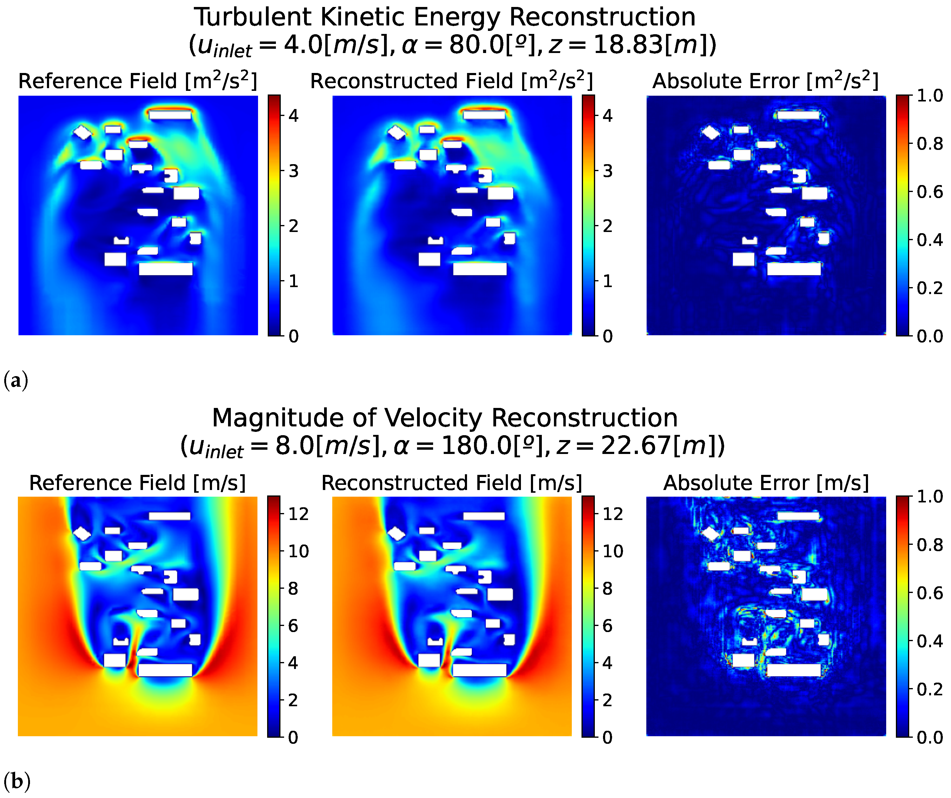
The first stage of the analysis evaluates the ability of the convolutional autoencoder to reconstruct the input flow fields on the validation dataset. Figure 4 shows the reconstructed turbulent kinetic energy (TKE) and velocity magnitude fields alongside the corresponding reference data. In both cases, the reconstructions reproduce the global structures of the flow with high accuracy. Error fields indicate that the average reconstruction error is very small (average normalized MAE of less than ${10}^{-3}$) across most of the domain. Localized regions of higher error, where normalized MAE is less than 0.05, appear near the wall boundaries, where the gradients are steeper and small-scale structures are more difficult to capture. Despite these localized discrepancies, the overall accuracy demonstrates that the CAE successfully encodes and decodes the dominant features of the flow.

5.2. Prediction with the CAE–DNN Model

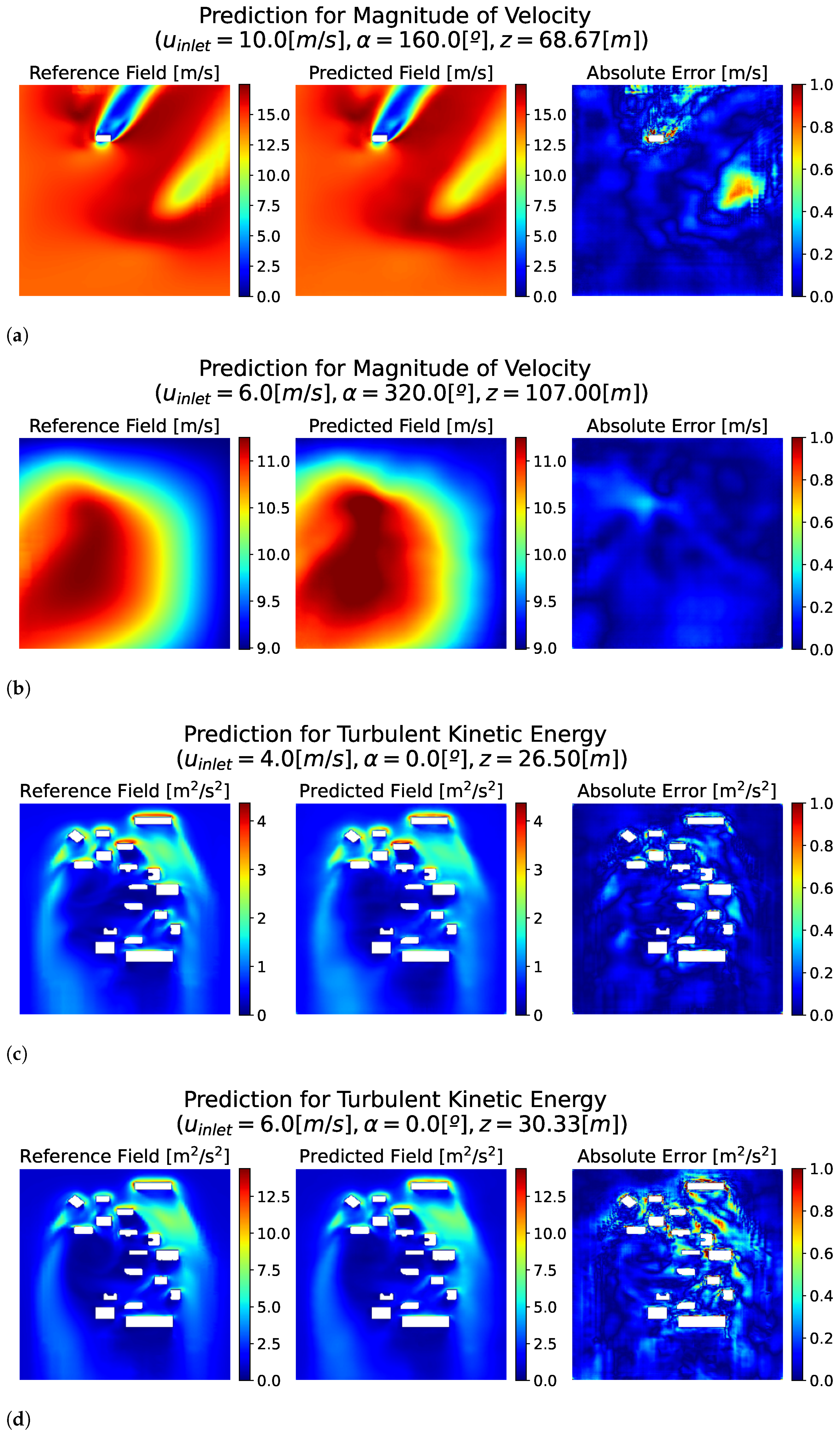
The second stage assesses the predictive capability of the combined CAE–DNN framework. The model was tested on a case not included in the training dataset, in order to evaluate its generalization ability. Figure 5 presents the predicted velocity magnitude and TKE fields, respectively, together with the reference (CFD-computed) fields, showing the corresponding absolute errors.

Similarly to the reconstruction results, the predicted fields closely match the reference data. The global structures of both TKE and velocity magnitude are well reproduced, demonstrating that the model is capable of learning the mapping from input conditions to flow field outputs. Error maps show that the average error remains very small across the domain, with slightly larger deviations again concentrated near the wall regions.

To further quantify the accuracy of the predictions, the error between each predicted slice and its corresponding ground truth was computed using the validation dataset. Three error metrics were evaluated: RMSE, MAE, and MSE. These errors were computed using normalized and de-normalized fields. The detailed values for both velocity magnitude and turbulent kinetic energy are summarized in

Table 4. Average and maximum errors for velocity magnitude and turbulent kinetic energy (TKE) using normalized and de-normalized values.

Velocity Magnitude
Metric	Average Error		Maximum Error
	Normalized	De-Normalized [m/s]	Normalized	De-Normalized [m/s]
MAE	0.0064	0.1341	0.0531	1.1080
RMSE	0.0099	0.2075	0.0765	1.5962
MSE	0.0001	0.0713	0.0058	2.5478
Turbulent Kinetic Energy (TKE)
Metric	Average Error		Maximum Error
	Normalized	De-normalized [${\mathrm{m}}^2$/${\mathrm{s}}^2$]	Normalized	De-normalized [${\mathrm{m}}^2$/${\mathrm{s}}^2$]
MAE	0.0035	0.1047	0.0105	0.3146
RMSE	0.0069	0.2062	0.0337	1.0121
MSE	0.0021	0.0625	0.0342	1.0244

. Physical error values can be obtained by multiplying by the corresponding scaling factor employed during the normalization process. In addition, Figure 6 shows the frequency distribution of the error values for each metric, providing further insight into the variability of the prediction errors across the validation set.

Overall, these results confirm that the proposed CAE–DNN framework can effectively predict complex urban flow fields, capturing both global patterns and localized variations with high fidelity.

The reduced computational cost of the predictive model is a major advantage: a single flow prediction requires approximately 0.03 s, compared to 120 s for a CFD simulation, corresponding to a speed-up of approximately 4000 times.

These results confirm that the predictive model can generate accurate flow predictions with a negligible error margin compared to CFD, while offering a significant speed-up, making it ideal for coupling with the path planning algorithm.

5.3. Path Planning Assessment Results

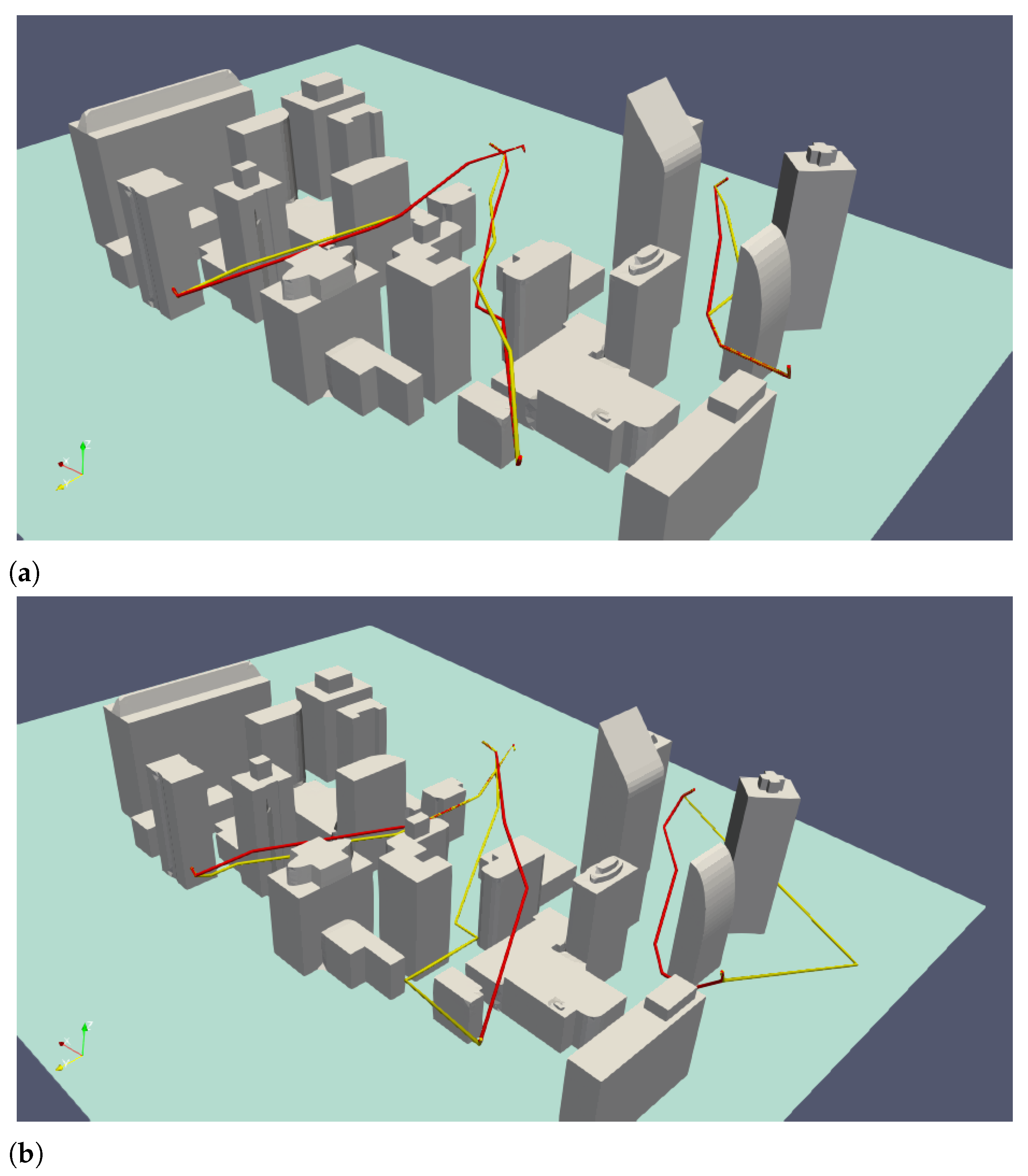
To evaluate the proposed trajectory optimization framework, two test cases were generated with the CAE–DNN surrogate model, each corresponding to different inlet conditions of the urban flow. The boundary conditions for these cases are summarized in

Table 5. Boundary conditions ($u_{\mathrm{inlet}}$ y ${\alpha }_{\mathrm{inlet}}$) for each tested case.

Case	${\mathit{u}}_{\mathbf{inlet}}$ [m/s]	$\mathit{\alpha }$ [°]
#1	6.5	225
#2	7.9	341

, which lists the inlet velocity magnitude and wind direction used as model inputs. In addition to these two boundary conditions, the surrogate model also predicted the vertical distribution of the flow: slices of the turbulent kinetic energy (TKE) field were generated at heights ranging from 0 to 100 m with a resolution of 1 m. This provided the required spatial information on TKE to be used as input for the path planning algorithm.

For each case, two candidate routes were considered, and multiple trajectories were obtained for each route by varying the maximum admissible turbulent kinetic energy ($TK{E}_{max}$). Figure 7a,b show representative examples of the resulting trajectories. As expected, the solutions diverge progressively as the turbulence threshold is reduced, yielding safer but less direct paths. Quantitative indicators summarizing these results are presented in

Table 6. Quantitative indicators for each trajectory under different TKE thresholds ($TK{E}_{max}=2.5{\mathrm{m}}^2/{\mathrm{s}}^2$ and $TK{E}_{max}=4{\mathrm{m}}^2/{\mathrm{s}}^2$) for the two predicted cases (TR denotes the turbulence kinetic energy threshold ($TK{E}_{max}$) applied in the trajectory planning process. P1, P2 and P3 denotes the three different paths).

Case	Parameter	P1		P2		P3
		TR 2.5	TR 4	TR 2.5	TR 4	TR 2.5	TR 4
#1	$\overline{k}$ (${\mathrm{m}}^2$/${\mathrm{s}}^2$)	2.39	2.56	2.38	2.65	2.34	3.03
	L (m)	180.21	179.28	163.60	163.50	129.30	125.99
	t (s)	0.0008	0.0008	0.0005	0.0005	0.0007	0.0007
#2	$\overline{k}$ (${\mathrm{m}}^2$/${\mathrm{s}}^2$)	2.47	2.63	2.43	2.87	2.44	3.21
	L (m)	197.92	183.35	175.70	165.30	163.00	136.50
	t (s)	0.1269	0.1904	0.0010	0.0007	0.0020	0.0004

, which reports the mean turbulent kinetic energy ($\overline{k}$), the length of the path (L), and the computation time (t) for each case. In all scenarios, computation time remained below one second per trajectory.

These results highlight the benefits of the proposed approach: the planner adapts routes to changing flow conditions, avoids regions of excessive turbulence, and maintains smooth, feasible trajectories while requiring negligible computation time. This combination of adaptability, safety, and efficiency demonstrates the potential of the framework for real-time UAV operations in urban environments.

6. Conclusions

The presented CAE–DNN surrogate demonstrates that high-fidelity urban wind fields can be approximated with both high accuracy and extreme speed. The model reproduces the principal flow structures and TKE patterns observed in CFD simulations while speeding-up the prediction by 4000×. These results show that a compact latent representation combined with a lightweight regressor is an effective strategy for compressing and reconstructing spatially complex aerodynamic fields for real-time use.

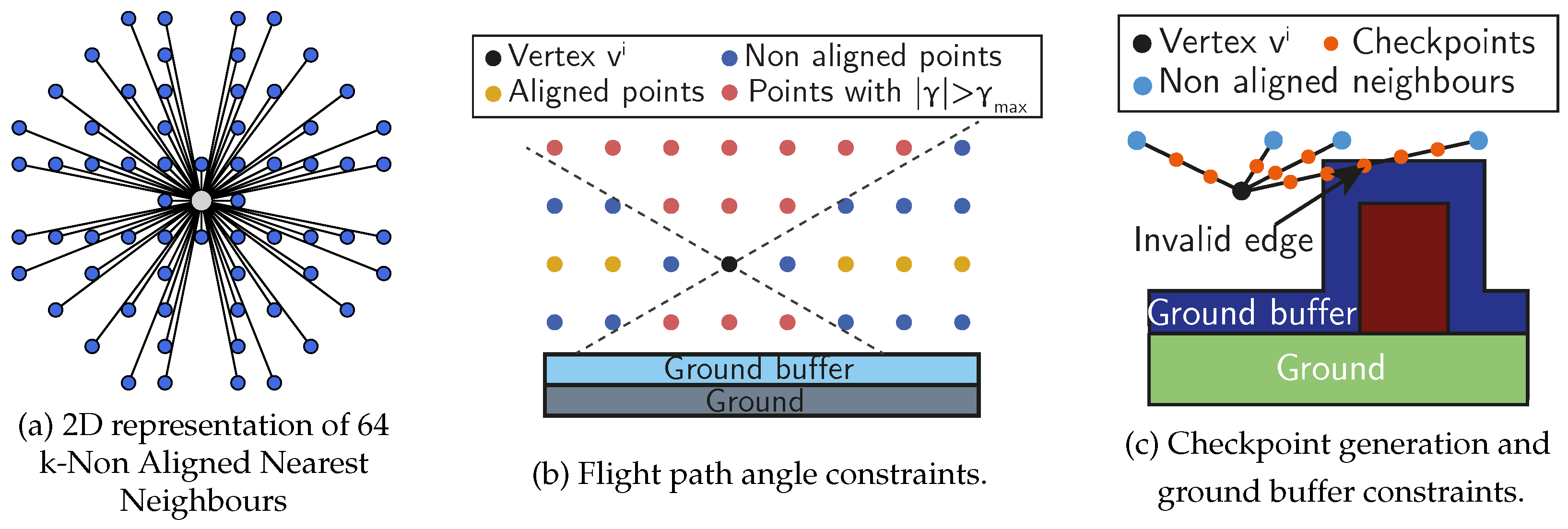
When coupled with the k-NANN airspace discretization and an A* planner that enforces heading and TKE traversability constraints, the surrogate enables adaptive, constraint-aware trajectory generation. The integrated pipeline converts raw flow predictions into operationally meaningful guidance: computed routes systematically avoid high-turbulence regions while remaining smooth and flyable. This closes the loop between environmental estimation and mission planning and demonstrates the practical value of embedding fast flow prediction in UAV navigation systems.

The two-stage training strategy (CAE followed by DNN) and the use of slice-based inputs proved effective for the benchmark scenarios considered, achieving low prediction errors and stable convergence. These results suggest that the current dataset provides a good balance between accuracy and computational cost. Beyond aerodynamic fidelity, we highlight the integration of surrogate predictions with energy-aware route optimization, where vehicle-specific power models enable quantifiable gains in efficiency. Ongoing methodological refinements, such as volumetric encodings and physics-aware losses, are expected to further enhance generalization in complex urban flows. Future work will explore the impact of CFD data diversity and quality on learning efficiency, aiming to minimize the number of required simulations without compromising reconstruction accuracy..

It is also important to acknowledge that, within the current framework, the UAV aerodynamic response is not yet explicitly modeled. The CFD results are incorporated into a strategic path planning system that defines optimal flight trajectories prior to operation. This system uses TKE values obtained from steady-state CFD simulations to compute efficient routes that avoid high-TKE regions prone to strong gust formation. Future work will focus on investigating vehicle–flow interaction effects to further evaluate the influence of TKE thresholds on flight safety.

In parallel, subsequent efforts will extend validation to diverse urban conditions, incorporate uncertainty quantification for risk-aware planning, and assess performance on embedded platforms. Collectively, these steps advance the path toward reliable, auditable, and operationally beneficial deployment of surrogate-assisted wind modeling for drone navigation.

Overall, the methodology provides a scalable foundation for fast wind estimation and UAV trajectory planning. By bridging data-driven models and CFD, and by integrating predicted flow into energy-aware and risk-aware planners, this framework can materially improve the safety, endurance, and operational efficiency of urban drones. With the recommended extensions and validations, it can evolve into a practical module for fleet operations, urban traffic management, and certification workflows, contributing to safer and more sustainable urban air mobility.