Highlights
What are the main findings?
- An efficient multi-object tracking algorithm is proposed, which integrates 2D object detection with unsupervised learning to achieve 3D object detection.
- A multi-object tracking algorithm using multi-level data association strategy is proposed, which effectively mitigates the impact of detection errors on tracking and prevents trajectory fragmentation caused by occlusion and other factors.
What is the implication of the main finding?
- The proposed detection and tracking algorithm is independent of high-performance GPU devices, making it advantageous for practical deployment. On low-cost unmanned system platforms, our algorithm can maintain strong stability.
- The proposed algorithm employs multi-sensor fusion to effectively address the problem of trajectory fragmentation in the absence of 3D information, maintaining high accuracy in complex scenarios.
Abstract
3D object detection and tracking technology are increasingly being adopted in unmanned ground vehicles, as robust perception systems significantly improve the obstacle avoidance performance of a UGV. However, most existing algorithms depend heavily on computationally intensive point cloud neural networks, rendering them unsuitable for resource-constrained platforms. In this work, we propose an efficient 3D object detection and tracking method specially designed for deployment on low-cost vehicle platforms. For the detection phase, our method integrates an image-based 2D detector with data fusion techniques to coarsely extract object point clouds, followed by an unsupervised learning approach to isolate objects from noisy point cloud data. For the tracking process, we propose a multi-target tracking algorithm based on multi-level data association. This method introduces an additional data association step to handle targets that fail in 3D detection, thereby effectively reducing the impact of detection errors on tracking performance. Moreover, our method enhances association precision between detection outputs and existing trajectories through the integration of 2D and 3D information, thereby further mitigating the adverse effects of detection inaccuracies. By adopting unsupervised learning as an alternative to complex neural networks, our approach demonstrates strong compatibility with both low-resolution LiDAR and GPU-free computing platforms. Experiments on the KITTI benchmark demonstrate that our tracking framework achieves significant computational efficiency gains while maintaining detection accuracy. Furthermore, experimental evaluations on the real-world UGV platform demonstrated the deployment feasibility of our approach.
1. Introduction
Autonomous navigation technology has gained significant attention in recent years, as it enables sensor-equipped unmanned ground vehicles (UGV) to perform a wide range of tasks, including data collection, environmental modeling, and monitoring [1,2]. An essential component of an autonomous navigation system is the real-time detection and tracking of obstacles. By fully considering the position, velocity, and historical trajectory of obstacles, the UGV can plan its actions more effectively, thereby preventing unintended collisions [3,4]. In addition, the era of intelligent systems has brought growing requirements for the perceptual and interactive capabilities of unmanned system equipment [5]. Therefore, as the working settings of the UGV become increasingly complex, the ability of UGV to perceive dynamic objects is becoming more and more important.
In the field of autonomous navigation, cameras and LiDAR are the most commonly used sensors for object detection and tracking [6]. In the commonly used tracking-by-detection framework, tracking algorithms typically first utilize neural networks to generate detection boxes, which are then associated with historical trajectories [7]. Early algorithms focus on 2D detection [8] and 2D tracking tasks, which use images to generate 2D boxes and trajectories for objects. In recent years, 3D LiDAR-based perception and navigation technologies have gained significant attention. On the one hand, LiDAR can accurately measure the distance between an obstacle and a UGV. On the other hand, the point cloud data provided by LiDAR offers detailed geometric information about the environment, which is highly beneficial for multi-object detection and tracking. While LiDAR provides significant advantages, it also presents great challenges. Unlike image data, point cloud data is not spatially continuous, and its distribution characteristics vary across frames [9]. Therefore, convolutional neural networks, which are commonly used for image processing, struggle to directly extract features from point cloud data. Correspondingly, multi-object tracking algorithms using point clouds also face several challenges in industrial applications.
The first challenge lies in the low efficiency of traditional detection algorithms, primarily caused by the sparsity and unstructured nature of the point cloud. The irregular distribution of point cloud data compels most object detection algorithms to convert it into alternative representations to facilitate processing by convolutional neural networks. For instance, some algorithms transform 3D point clouds into 2D images, which are subsequently processed using convolutional networks [10,11]. However, this dimensionality reduction results in significant information loss. Consequently, these methods typically use multiple neural networks to extract features from various perspectives (such as bird’s eye view, frontal view, and images) [12]. The concurrent execution of multiple networks severely compromises computational efficiency. Another common approach involves representing the 3D space using uniformly distributed cuboids or voxels, followed by object detection via 3D convolutional networks, with each voxel serving as the basic unit [13,14,15]. This method also suffers from inefficiency due to the need to traverse a large number of empty voxels. Although some studies have proposed algorithms that operate directly on raw point clouds, their performance and efficiency on large-scale data remain inadequate [16,17]. As a result, these methods still fall short of meeting the real-time requirements of autonomous navigation, which often involves processing outdoor point clouds over extensive areas.
The second factor limiting the practical application of multi-object tracking algorithms is that the existing data association based on single-sensor input is not reliable enough. Weng et al. proposed the AB3DMOT algorithm [18], which was regarded as a benchmark method in the 3DMOT field. Their method uses Intersection over Union (IoU) to represent the similarity between detection boxes and prediction boxes, and then uses the Hungarian algorithm and Kalman filtering to complete trajectory updating. The tracking performance of this kind of algorithm is strongly correlated with the precision of the detected bounding boxes. However, the complexity of point cloud data makes accurately generating 3D detection boxes a challenging task in practical industrial applications. Moreover, in real-world environments, the rapid changes in object pose often hinder the ability of 3D IoU to accurately quantify the similarity between detection results and trajectories [19]. Some methods integrate multi-sensor data during the detection phase to enhance tracking performance by improving the accuracy of 3D boxes [20]. Some other methods, such as the ByteTrack algorithm [21,22], employ a staged data association approach based on detection confidence scores. Nonetheless, these methods fail to address the problem at its core, since similarity is still computed based on 3D bounding box comparisons. Consequently, they often suffer from reliability problems in real-world scenarios.
Another critical yet frequently overlooked challenge is the heavy reliance of most existing tracking algorithms on high-performance GPUs and advanced sensors, which severely limits their deployment on cost-constrained UGV platforms. Mobile UGVs must handle multiple tasks simultaneously, including perception, localization, and planning, leaving limited computational resources and processing time for object tracking. Additionally, some UGVs are not equipped with high-line LiDAR, which can significantly degrade the performance of point cloud neural networks. Most existing studies focus on employing complex neural networks to improve algorithm performance on public datasets. The impressive results reported by these algorithms are primarily dependent on 64-line LiDAR sensors and high-performance GPUs. Shi et al. [23] conducted experiments on a desktop equipped with an i9 CPU and an RTX 3090 GPU. Ye et al. [13] conducted experiments on a 2080Ti GPU. The inference time of MV3D-Net for one image was around 0.36 s on a Titan X GPU [12]. On UGVs equipped with only a CPU and 32-line LiDAR, these algorithms often fall short in both accuracy and efficiency, and in some cases, may fail to operate altogether. In real-world applications, limitations in cost, size, and thermal management prevent the control system from enhancing algorithm performance by simply adding more computational hardware [24]. This dilemma causes many 3D MOT algorithms to struggle to meet the needs of autonomous navigation.
In this work, we propose a novel 3D object detection and tracking method designed for low-cost UGVs. To improve the algorithm’s efficiency, we refrain from using point cloud neural networks for 3D feature extraction. Instead, we first identify the region where the object is located, and then distinguish the object from noise points using point cloud clustering. To prevent the fragmentation of tracking trajectories caused by 3D detection errors, we propose a multi-object tracking algorithm that employs a multi-level data association strategy. On the one hand, we compute similarity using 2D IoU and 3D Mahalanobis distance, thereby mitigating the impact of detection errors in any single dimension. On the other hand, we perform grouped data association: first handling objects with both 2D and 3D information based on their confidence scores, and then conducting a third round of association specifically for objects that only contain 2D information due to clustering failures. The proposed tracking algorithm effectively mitigates the impact of detection errors on tracking performance. Section 6 demonstrates that our method not only performs well on public datasets but also adapts to low-cost industrial computers and 32-line LiDAR, which is often unachievable by many existing MOT algorithms. The main contributions of our work are as follows:
- (1)
- We propose an efficient multi-object detection method designed for low-cost UGVs. Our method combines image-based object detection techniques with point cloud data processing methods to achieve 3D object detection. The simplicity of the network enables our algorithm to run efficiently in a CPU environment, while the clustering-based feature extraction ensures compatibility with 32-line LiDAR data.
- (2)
- We propose a tracking algorithm using a multi-level data association strategy, which effectively mitigates the impact of detection errors on tracking performance. In terms of similarity computation, we integrate both 2D and 3D detection results. For data association, we group the detections by first associating those with high confidence and complete information, and then perform a dedicated third matching step to handle cases where point clouds cannot be successfully clustered. Even when the 3D detector cannot provide accurate results at certain moments, our tracking process maintains high accuracy with image data.
- (3)
- We conduct extensive comparative experiments on public datasets and a real UGV platform. The results demonstrate that our algorithm operates efficiently and reliably during the autonomous navigation process.
The remainder of this paper is organized as follows. Section 2 reviews the related work on multi-object detection and tracking. Section 3 presents the overall framework of the proposed method. Section 4 and Section 5 detail the principle of the proposed detection and tracking algorithm, respectively. In Section 6, the proposed method is evaluated on both the KITTI MOT dataset and a real UGV platform to experimentally validate its effectiveness. Finally, some conclusions are drawn in Section 7.
2. Related Work
Multi-object tracking algorithms can be divided into two paradigms, which are tracking by detection (TBD) and joint detection tracking (JDT) [6]. The former divides detection and tracking into two independent tasks, while the latter achieves end-to-end tracking. Consistent with prevailing methodologies, our approach implements the Tracking-by-Detection (TBD) framework. This section provides a comprehensive review and analysis of relevant literature.
2.1. Multi-Object Detection
The unique characteristics of point cloud data necessitate that 3D object detection algorithms address two critical aspects: the architecture of neural networks and the representation methods for point cloud data. Common LiDAR-based detection algorithms can be categorized into projection-based methods, voxel-based methods, and point-based methods. Projection-based methods focus on viewing the point cloud data from a specific perspective, such as a front view (FV) [11,25] or bird’s eye view (BEV) [26]. These methods convert 3D point clouds into 2D images and then use convolutional layers to extract features, avoiding the complexities of processing three-dimensional data. However, the information loss during the projection process inevitably affects detection accuracy. Voxel-based methods format the irregular point cloud data into a neat matrix, facilitating feature extraction using 3D convolutional networks [15]. To avoid wasting computational resources by traversing empty voxels, subsequent voxel-based algorithms have made improvements in voxel partitioning strategies [14] and neural network structure [27]. However, voxel-based methods still cannot avoid the loss of the natural geometry of points and require complex regularization processes [28]. Qi et al. introduced PointNet [16], a point-based architecture that utilizes symmetric functions to effectively process unordered point cloud data, enabling end-to-end object detection. However, point-based approaches exhibit limitations in both computational efficiency and detection accuracy when handling large-scale point cloud datasets [29].
The challenges of single-modal object detection have driven extensive research into multi-modal object detection algorithms. The key distinction among these algorithms lies in how and when the data from different sensors are fused. F-PointNet [30] efficiently identifies regions of interest in the point cloud by leveraging a mature 2D object detector and data fusion technology, and subsequently generates 3D detection results using PointNet. MVX-Net [31] integrates the results of a 2D detector with the point cloud data, which are then fed into VoxelNet, resulting in improved accuracy over the original VoxelNet model. These algorithms adopt the strategy of early fusion. In contrast, MV-3D [12] introduces an intermediate fusion approach, where proposal regions are initially generated separately from the image, bird’s eye view, and front view, and then fused using networks for bounding box prediction. Other intermediate fusion methods share a similar structure but differ in their point cloud feature extraction techniques. Additionally, some algorithms use a late fusion strategy [32,33], where 2D and 3D bounding boxes are independently generated from the image and point cloud data, and subsequently fused to enhance detection accuracy. However, regardless of the fusion strategy designed, these methods require multiple complex feature extraction networks and fusion networks. Therefore, while multi-sensor fusion can enhance detection accuracy, the computational burden of processing data from multiple sensors cannot be overlooked.
It can be observed that current research primarily focuses on the innovative design of neural network models to enhance object detection accuracy. Undoubtedly, these complex algorithms have shown improved performance in terms of metrics, demonstrating significant potential for applications in complex tasks such as small object detection. However, the complexity of these algorithms limits their practical applicability. For UGVs, real-time updates of the trajectories of surrounding pedestrians are more critical than the detection of pedestrians at a distance. On the other hand, in real-world applications, controlling hardware costs is just as important as achieving high accuracy. Most current detection and tracking algorithms rely on high-performance GPUs and high-line LiDAR sensors. For example, References [34,35] used an RTX 3090 GPU, while Reference [33] used an RTX 3080 GPU. However, in real-world applications, limited hardware capabilities often prevent these algorithms from achieving the expected efficiency and accuracy.
2.2. Multi-Object Tracking
Within the TBD paradigm, the tracking process aims to establish one-to-one correspondence between detection outputs and existing trajectories, followed by subsequent trajectory updates. Bewley et al. introduced the SORT algorithm [7], an efficient framework that generated predicted boxes from historical trajectories and then used the Hungarian algorithm and IoU to match predicted boxes with detection boxes. Weng et al. extended SORT to three dimensions and proposed the AB3DMOT algorithm [18], which was regarded as a benchmark method in the 3DMOT field. However, the algorithm’s accuracy often falls short of meeting practical application requirements. When objects are difficult to detect due to occlusion or other factors, the accuracy can significantly decrease.
To improve the accuracy of tracking algorithms, researchers have made enhancements to various components of the tracking process. Hu et al. [36] enhanced the state prediction process by introducing an LSTM-based object velocity learning module, which aggregated long-term trajectory information to achieve more accurate motion extrapolation. Zhang et al. [22] proposed a complementary 3D motion prediction strategy that utilized the object velocity predicted by the detector for short-term association and adopted the Kalman filter for long-term association when objects were lost and reappeared. While state estimation model refinement enhances tracking precision, it remains ineffective in mitigating the adverse effects of detection errors on tracking performance. Some studies perform data association in stages based on the confidence of detection boxes or tracklets [21,37], achieving better performance in cases of partial object occlusion. However, if the accuracy of the 3D bounding boxes is poor, the performance of these algorithms will be severely impacted. Cheng et al. [19] improved the similarity calculation function by extracting features from the high-dimensional space of 3D bounding boxes and then calculating the feature distance between detection and predicted boxes to represent similarity. However, the complex feature extraction process in their algorithm further increased the computational burden on the control system.
Overall, most current multi-object tracking algorithms heavily depend on precise 3D bounding boxes. Regardless of the data association strategy employed, these algorithms universally require accurate 3D bounding box information to compute similarity metrics. Consequently, if the detection algorithm fails to provide reliable 3D information at any point, the tracking trajectories are susceptible to fragmentation. Therefore, these algorithms may struggle to achieve the desired performance in practical applications.
3. System Framework
In this work, we focus on the study of 3D multi-object detection and tracking algorithms, emphasizing improvements in computational efficiency and deployability on low-cost UGV platforms. The overall framework of our method is illustrated in Figure 1. Our algorithm follows the tracking-by-detection paradigm, where we first perform object detection using both image and point cloud data. Then, the detected objects are matched to existing trajectories based on their 2D and 3D information. To address the limitations of low-cost devices, we design a novel data fusion-based object detection algorithm. Additionally, we enhance the critical data association process to improve the performance of the tracking system built on our detection algorithm.
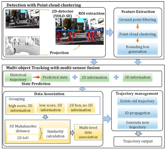
Figure 1.
Overall framework of our method.
In practical industrial applications, it may be challenging for UGVs to be equipped with high-performance and expensive GPUs and sensors. On industrial computers with only a CPU, complex point cloud neural networks may struggle to run efficiently. Furthermore, when using 32-line LiDAR as input, some neural networks may face difficulties in extracting 3D features. Therefore, we combine image-based 2D object detection techniques with point cloud processing methods to propose an efficient 3D object detection algorithm. Our algorithm first projects the point cloud onto the image and then extracts the region of interest in the point cloud based on the 2D detection boxes. For the point cloud regions containing objects and noise, we perform ground point filtering and clustering operations, ultimately generating 3D detection boxes as the output. In this process, we avoid using complex point cloud neural networks, making our algorithm more suitable for low-cost UGV platforms.
Consistent with the mainstream tracking algorithm, our method consists of three main steps: prediction, data association, and trajectory lifecycle management. Since the tracking process does not significantly contribute to runtime overhead, our primary innovation focuses on enhancing the data association process, thereby optimizing the tracking algorithm for better compatibility with our detector and the engineering application. In practical applications, missed detections and false positives are inevitable, and this issue is further exacerbated on cost-constrained UGV platforms. Conventional multi-object tracking algorithms are highly susceptible to this issue, often resulting in fragmented trajectories. To address this, we integrate multi-modal data during the data association process. Specifically, we evaluate similarity using the Mahalanobis distance between the 3D detection box and the predicted box. To address situations where 3D information is unavailable, we propose a multi-level data association strategy specifically designed to handle such cases, thereby mitigating trajectory fragmentation. In this process, the detection results are divided into three groups: the first and second groups both contain complete information but differ in confidence levels, while the third group lacks 3D information. Conventional tracking algorithms typically discard the third group of targets; however, our method employs a dedicated third round of data association to handle such cases, thereby preventing trajectory fragmentation. Specifically, we leverage the targets’ 2D information for association, ensuring that their identifiers remain consistent when they are re-clustered in the LiDAR coordinate system. The combined effect of data fusion and association strategies ensures robust reliability in practical engineering scenarios.
4. Detection with Point Cloud Clustering
The key advantage of our object detection process lies in its independence from powerful computing devices and high-line LiDAR. It consists of five main steps: performing 2D object detection, extracting regions of interest (ROIs) from the point cloud, removing ground points, applying clustering, and generating 3D bounding boxes. The first step uses the 2D detector to obtain the objects’ class, location, and confidence score. The remaining steps focus on extracting the point cloud corresponding to the detected object. Since our tracking algorithm uses 2D IOU and 3D Mahalanobis distance in the data association process, our detection process outputs both the 2D bounding boxes and the 3D spatial coordinates of all objects. Any unused information will not be computed during the detection process, which can further enhance the algorithm’s operational efficiency.
4.1. 2D Detector
Compared to point clouds, RGB images provide richer color and contextual information in a more compact format, making them easier to process with neural networks. In addition, the rich color and texture information they provide contribute to improved detection accuracy. Given the notable variations in efficiency, accuracy, and hardware demands across different 2D object detection algorithms, the choice of a suitable detection method is crucial for real-world applications. In this work, we use the YOLO algorithm for 2D object detection, as it provides end-to-end detection and demonstrates strong performance in both efficiency and accuracy. Furthermore, we integrate Squeeze-and-Excitation (SE) modules into YOLO, which produces significant performance improvements at minimal additional computational cost. The SE module, as a channel attention mechanism, enhances the network’s focus on important features by adaptively adjusting the weight of each channel, while suppressing redundant information, thereby improving the accuracy of the detector. Final outputs of the 2D detector can be formulated as
where represents the j-th detection bounding box in the image frame at time t, represent the horizontal and vertical coordinates of the four vertices of the detection box, is the detection confidence score, and denotes the category of the object.
4.2. ROI Extraction
After obtaining the 2D detection box, our algorithm extracts the point cloud ROI by utilizing the relative position relationship between the camera and the LiDAR. As shown in Figure 2, this process involves three coordinate systems: the LiDAR coordinate system, the camera coordinate system, and the pixel coordinate system. The LiDAR and camera coordinate systems are 3D spatial coordinate systems with the origin at the locations of the respective sensors, while the pixel coordinate system is a 2D coordinate system corresponding to the RGB image.
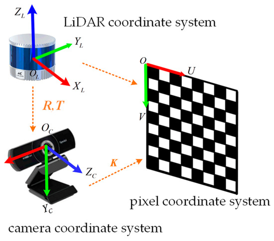
Figure 2.
The three coordinate systems in the data fusion process.
To obtain the point cloud region corresponding to the 2D detection box, the point cloud data in the LiDAR coordinate system must be projected onto the pixel coordinate system. Since the LiDAR and camera are mounted at different positions on the vehicle, the point cloud needs to be transformed into the camera coordinate system first. This process can be formulated as
where , , and represent the coordinates in the camera coordinate system, and , , and represent the coordinates in the LiDAR coordinate system. and represent the rotation and translation matrices, respectively, that define the transformation between the two coordinate systems. After the transformation from the LiDAR coordinate system to the camera coordinate system, the points can be further projected into the pixel coordinate system using the corresponding camera intrinsic calibration parameters. This process can be formulated as
In Equation (3), (, ) represents the coordinate of a point in the point cloud within the pixel coordinate system, and is the intrinsic matrix of the camera. The transformation matrices , , and are obtained through the sensor calibration process, which is a necessary step before running any multi-sensor fusion algorithm. The camera intrinsic calibration process provides the intrinsic reference matrix , while the joint calibration of the camera and LiDAR provides the spatial transformation matrices and .
Equations (2) and (3) define the transformation between the LiDAR and pixel coordinate systems, which makes it possible to project 3D point cloud data onto the 2D image space. The subsequent step involves identifying potential object points in the point cloud by evaluating their projected locations within the pixel coordinate system.
For each detection box , if the confidence score exceeds a predefined threshold, it is likely to contain a valid object. Consequently, the points falling within these boxes is considered to belong to the ROI point cloud. The ROI point cloud can be formulated as
In Equation (4), represents the j-th region of interest in the point cloud at time t, which is associated with detection box , and is the i-th point contained in . As described in Equation (5), the location of each point in within the pixel coordinate system is constrained to lie inside the detection box . The set represents the output of the ROI extraction process, which includes the object point cloud along with some background noise.
It is worth noting that the accuracy of the 2D detector we use meets the practical requirements of autonomous navigation. This ensures that the size and position of the 2D bounding boxes are generally well aligned with the objects the vehicle is focused on. In other words, the detection boxes do not include excessive non-object pixels. Hence, the point cloud after rough extraction contains a high proportion of object points, which guarantees the feasibility of subsequent feature extraction.
4.3. Feature Extraction in Point Clouds
The 2D detector selects both the object and noise pixels, resulting in the ROI point cloud containing both object points and points of the surrounding environment, as shown in Figure 3. In outdoor environments where UGVs operate, the objects to be detected are typically pedestrians, cars, and other similar objects, while noises in point clouds mostly consist of ground points and background features. Typically, points of these features and objects exhibit significant differences in their spatial distribution characteristics. The height of ground points is significantly lower than that of other features, while background features, such as buildings, have a different depth compared to the objects awaiting detection. Thus, our algorithm employs an unsupervised learning approach to classify the point cloud: it first removes ground points, then performs clustering, and ultimately selects the object point clouds. Compared to algorithms utilizing point cloud neural networks, our algorithm demonstrates superior efficiency. Furthermore, it excels at processing 32-line point cloud data. Consequently, our algorithm offers greater advantages in practical applications, particularly on low-cost devices.
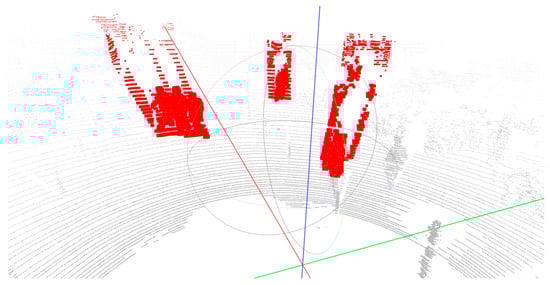
Figure 3.
The point cloud extracted from the 2D bounding box. The red part in the represents the point cloud corresponding to the area within the 2D detection box in 3D space, while the gray part denotes the remaining points. The red, green, and blue lines are the x-, y-, and z-axes of the point cloud coordinate system, respectively.
4.3.1. Ground Point Filtering
Ground points have two distinguishing features: (1) they lie on the same horizontal plane, (2) their Z-coordinates, when negated, are roughly equal to the height at which the LiDAR is mounted. Our algorithm searches for points that exhibit these features, starting from the point closest to the LiDAR. In the subsequent step, we evaluate whether pairs of potential ground points belong to the same horizontal plane. We begin by examining the first feature. As illustrated in Figure 4, consider two adjacent LiDAR beams intersecting the object at points A and B, whose coordinates are and . Let the height difference between points A and B be , and their distance in the XOY-plane be . The angle formed between the line connecting points A and B and the horizontal plane can be computed as
Theoretically, if point A and B satisfy the second condition, the angle should be negligible. In practice, due to possible ground slope and sensor measurement errors, we allow tolerance. Specifically, point A and B are considered to meet the second feature if . If the vertical coordinates of points A and B are numerically close to the installation height of the LiDAR, they are considered as ground points. By iterating through all points and filtering out those identified as ground points, we obtain a refined point cloud that retains only background elements and objects of interest.

Figure 4.
Schematic diagram of ground points extraction. The red lines represent the laser beams emitted by the sensor, and the orange circles mark the points where the beams hit object surfaces.
4.3.2. Point Cloud Clustering
After filtering out the ground points, we use the DBSCAN (Density-Based Spatial Clustering of Applications with Noise) algorithm to extract object point clouds from the ROI point cloud. The DBSCAN algorithm can cluster point cloud clusters of arbitrary shapes within noisy data, aligning well with the requirements of our application.
As shown in Figure 5, DBSCAN algorithm divides the points in the data into three categories, which are core points, boundary points, and noise points.
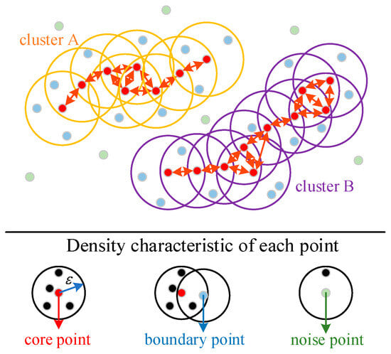
Figure 5.
Schematic diagram of point cloud clustering. The points within the orange and purple circles correspond to two different classes. The red arrows connect a sequence of core objects that are density-reachable. Each blue boundary point within the same circle is directly density-reachable from the red core point, and any two blue boundary points within the same circle are density-connected to each other.
- Core points: A point p is classified as a core point if the number of points q within its neighborhood exceeds a predefined threshold . It can be formulated as . The neighborhood radius and the threshold are input parameters for the algorithm. In Figure 5, circles represent the neighborhood radius, and red points indicate the core points.
- Boundary points: Points that lie within the neighborhood of a core point but are not core points themselves are referred to as boundary points.
- Noise points: Points that are neither core points nor located within the neighborhood of any core points are classified as noise points.
DBSCAN defines three fundamental concepts to characterize relationships between these points: directly density-reachable, density-reachable, and density-connected [38]. A point q is directly density-reachable from a point p if q lies within the ε-neighborhood of p, and p is a core point. A point q is density-reachable from p if there exists a chain of core points {p1, p2, …, pk}, with p1 = p and pk = q, where each point is directly density-reachable from the previous one. This relationship is asymmetric. Two points p and q are density-connected if there exists a point o from which both are density-reachable. These definitions allow DBSCAN to discover clusters of arbitrary shapes and effectively identify noise based on local point density. All density connected points are considered to belong to the same cluster point cloud. After inputting the point cloud data into the DBSCAN algorithm, several clusters of denoised point clouds can be obtained:
In Equation (9), represents the output of the clustering algorithm, which contains n clusters of point clouds of different categories. denotes the clustering process, and is the input of the clustering algorithm. Since the object within each detection box corresponds to the majority of the pixels, the associated point cloud within the corresponding region is also expected to contain the highest density of points representing the object. Therefore, for the clustered point cloud, our algorithm selects the cluster with the largest number of points as the object point cloud. For the object point cloud, a 3D bounding box can be fitted to its boundary. However, since our tracking algorithm does not rely on 3D IoU for similarity computation, the 3D information provided by the detection module to the tracking module in this work is limited to the coordinates of the center of each detected object.
5. Multi-Object Tracking with Multi-Sensor Fusion
The ultimate task of the multi-object tracking algorithm is the updating and management of trajectories. In tracking-by-detection frameworks, Kalman filtering is commonly used for updating trajectory states, with real-time detection results serving as the observation data. In this process, the algorithm needs to obtain predicted data based on historical trajectories. More importantly, it must perform a one-to-one matching between the predicted data and the observation data. Current mainstream algorithms follow the SORT framework, which performs data association using the IoU between the predicted and detected bounding boxes. However, when 3D detection results are inaccurate, the tracking process may not proceed smoothly. In fact, errors in 3D detection are likely to occur in real-world complex scenarios, especially when the LiDAR has a low number of scan lines. Therefore, current general-purpose 3D multi-object tracking algorithms may struggle to achieve the desired performance in real-world tasks.
In this work, we propose a multi-level data association strategy based on multi-sensor data fusion, which mitigates the impact of detection errors on tracking performance. Our tracking algorithm comprises three components: prediction, data association, and trajectory lifecycle management. In the data association stage, we calculate the similarity between detection results and predicted results using a weighted sum of 2D IoU and 3D Mahalanobis distance. Then, based on the similarity, the Hungarian algorithm is used to match trajectories with detection results. Unlike other algorithms that only use 3D IoU to calculate similarity, our algorithm can associate detection results with trajectories even in the absence of 3D detection boxes, preventing trajectory fragmentation. Furthermore, we adopt a grouped matching approach, where detection results are matched in batches according to the confidence levels and the availability of 3D information. This further enhances the accuracy of our algorithm.
5.1. State Prediction
Since 2D IoU and Mahalanobis distance are used during the data association process, both the predicted results and detection results must include the following information:
In Equation (10), is the information of the j-th object detected by our algorithm at time t. It includes the 2D bounding box, object category, confidence score, and the center coordinates of the corresponding object point cloud. During the tracking process, this information serves as the observation data for the state update step.
For a given trajectory, the object category and the detection box size at each historical time step are known. During the prediction stage, we assume that the size of the 2D bounding box corresponding to the object at time t remains the same as at time t. Therefore, only the object’s center position in both the image coordinate system and the LiDAR coordinate system needs to be estimated for time t. Consistent with the AB3DMOT algorithm, our approach employs a constant velocity model to predict the object’s position. This process can be formulated as
where is a prior estimate of the i-th object’s center position at time t in the LiDAR coordinate system. It is important to note that the i-th object refers to the object associated with the i-th trajectory. represent the object’s velocity components along the three spatial axes, and denotes the time interval. It can be observed that we do not use the object’s angular velocity information in the prediction process. This is because previous studies have shown that including angular velocity does not significantly improve prediction accuracy [39]. Given the difficulty of estimating the object’s yaw angle, using angular velocity for position estimation may, in fact, reduce accuracy. Once the 3D center position of the object is estimated, its complete spatial information can be further derived. This process can be expressed as
Equation (12) provides an estimation of the boundary coordinates of the bounding box at time t. Here, represents the estimated center position of the i-th object at time t in the pixel coordinate system, which can be computed based on the estimated 3D coordinates using Equations (2) and (3). and represent the width and height of the detection box at time t, respectively. Equation (13) defines as the final predicted state of the i-th object at time t, where all variables retain the same meanings as in Equation (10), except for differences in subscripts and the time index. It is worth noting that these states are derived from the historical data of the i-th trajectory. Consequently, both the confidence score and the object category remain the same as in the previous time step.
5.2. Multimodal Data Association
Based on the characteristics of our multi-object detection algorithm, we propose a multimodal data association method that integrates 2D and 3D detection results. Unlike conventional algorithms, our method calculates the similarity matrix using both image and point cloud data. Furthermore, it performs data association in batches based on the 2D detection confidence scores. The combination of the similarity calculation method and the matching mechanism enables our algorithm to reduce the impact of detection errors on tracking accuracy.
Similarity calculation: For 2D and 3D detection results, we employ distinct methods to calculate the similarity between detected and predicted objects. Since the 2D detector can output accurate bounding boxes, we calculate the similarity between the 2D detection results and predicted results using the IoU of the bounding boxes. This process can be formulated as
where is the similarity between the i-th 2D detection result and the j-th predicted result, represents the area of the prediction box, represents the area of the prediction box. The larger the similarity is, the closer the predicted result is to the actual detection result, and the more likely they belong to the same trajectory. More specifically, and can be derived from the boundary coordinates of Bounding the box contained in and , respectively.
Unlike 2D bounding boxes in images, 3D cuboid bounding boxes in 3D space additionally require the acquisition of the objects’ pose angles and depth information. However, pedestrians and cars exhibit significant uncertainty in both the temporal and spatial dimensions of their poses. Consequently, generating accurate 3D bounding boxes is a considerable challenge for both detection and prediction phases. In this context, it is not advisable to continue using 3D IoU to calculate similarity. Consequently, we employ the Mahalanobis distance between the detection and prediction results as a measure of similarity. This process can be formulated as
In Equation (15), represents the Mahalanobis distance between the detection and the prediction, is the 3D observation matrix, is the noise covariance matrix, and represent the 3D coordinates of the detection result and the prediction result, respectively. In Equation (16), denotes the 3D similarity. The final similarity matrix can be obtained by weighted summation of these two similarity matrices, and the specific calculation formula is as follows
Matching strategy: Our 3D detector first generates 2D detection boxes and then extracts features within these boxes. The output detection results can be categorized into three classes. The first class consists of objects that are most reliably detected, characterized by complete 3D information and a confidence score above the threshold. The second class includes objects that may be partially occluded, resulting in confidence scores below the threshold; however, they can still be clustered and thus retain complete 3D information. The third category of objects can be detected in images; however, due to factors such as distance and occlusion, the corresponding point clouds are too sparse to form clusters. As a result, these objects contain only 2D detection information and lack 3D information. If the first two categories of objects are treated equally using the Hungarian algorithm, the tracking accuracy deteriorates. Moreover, if the third category of objects is directly discarded, they will be regarded as new objects once they are re-clustered, leading to fragmented tracking trajectories. Therefore, we propose a multi-level data association strategy to address this problem.
In the data association process, we initially apply the Hungarian algorithm to match objects from the high-confidence group with all available trajectories. Subsequently, the remaining trajectories are matched with the results from the low-confidence group. In both matching stages, we use the overall similarity as the input to the Hungarian algorithm. Finally, the third group of objects is associated with the remaining trajectories, where 2D IoU is used as the similarity measure during this process. Since the transformation between the camera and LiDAR coordinates is constant, maintaining consistent object IDs in the image ensures that the correct IDs can be reassigned when objects inside the 2D detection boxes are re-clustered. Even when the 3D feature extraction for certain objects is suboptimal, our algorithm can leverage 2D detection boxes to refine the tracking results. As a result, our data association process is well-suited to our detector.
5.3. Trajectory Management
After completing data association, the tracking algorithm utilizes detection results to update and maintain existing trajectories. During this process, the algorithm addresses three categories: successfully matched pairs, unmatched detection results, and unmatched trajectories. Accordingly, the algorithm executes three operations: trajectory updating, new trajectory initialization, and old trajectory removal.
Trajectory updating: For successfully matched pairs, the corresponding trajectories are updated using Kalman filtering. In the previous steps, all detection and prediction data have already been obtained. Assume that the Hungarian algorithm matches the i-th prediction with the j-th detection, indicating that they belong to the same object. The state updating process of the trajectory can be formulated as
where is the prior state of the object at time , is the posterior state the object at time , is the Kalman gain, is the observation of the object, and is the observation matrix. By integrating into the trajectory, the algorithm finalizes the update of the corresponding trajectory.
New trajectory initialization: In the data association process, certain detection bounding boxes exhibit high confidence levels yet remain unmatched to existing trajectories. These detections likely represent newly emerged objects, necessitating the initialization of new trajectories. However, to avoid tracking errors induced by detection inaccuracies, our algorithm refrains from immediately outputting newly initialized trajectories. These potential trajectories are only confirmed and output as new trajectories upon successful matching with detection bounding boxes in the subsequent data association cycle.
Old trajectory removal: Trajectory objects that fail to match any detection objects in data associations are typically assumed to have exited the vehicle’s detection range. However, in complex and dynamic environments, such mismatches may also result from long-term occlusion, causing the detector to miss previously tracked objects. To distinguish between objects that have left and those missed due to occlusion, the tracker employs a deletion threshold of 30 frames. This prevents the premature removal of trajectories, thereby avoiding trajectory fragmentation. Specifically, if a trajectory object fails to match any detection object over 30 consecutive frames, it is deemed to have exited the vehicle’s vicinity and is removed from the trajectory set, excluding it from further data association.
6. Experiments and Results
In this section, we provide a comprehensive evaluation of our algorithm’s performance in terms of accuracy and efficiency. For accuracy evaluation, we compare the outputs of our algorithm with those of commonly used 3D object tracking methods on publicly available datasets. Regarding efficiency, we deployed both our algorithm and the comparative algorithms on an actual UGV platform, comparing their execution times. Finally, we conducted multi-object tracking experiments in real-world scenarios using our unmanned vehicle, which is equipped with a CPU and a 32-line LiDAR, but no GPU. The experimental results demonstrate that our algorithm offers significant advantages on low-cost devices.
6.1. Datasets and Platform
The accuracy evaluation experiments are conducted on the KITTI 3D multi-object tracking dataset. The KITTI dataset consists of 21 training sequences and 29 testing sequences, providing both image and LiDAR data. These datasets are primarily composed of urban and highway environments, featuring numerous pedestrians and a wide range of vehicles. Since the ground truth for the KITTI test set is not publicly available, we follow the approach in references [18,19,20], dividing the training set into a training subset and a validation subset. Specifically, we use sequences 1, 6, 8, 10, 12, 13, 14, 15, 16, 18, 19 as the val set to compute the multi-object tracking metrics, and other sequences as the train set.
The efficiency evaluation experiments are conducted on a real UGV platform, which is equipped with an industrial computer along with sensors such as a LiDAR and a camera, as illustrated in Figure 6. The industrial control computer is not equipped with a GPU. For the specific efficiency evaluation, we will conduct tests using an Intel Core i5-12600TE CPU and an i7-9750H CPU. During autonomous navigation, the industrial computer may need to simultaneously handle tasks such as object detection, localization, and path planning. Therefore, the computational efficiency of each algorithm is critically important.
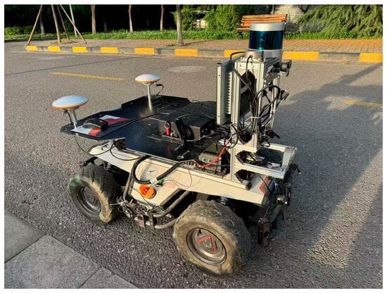
Figure 6.
Our UGV platform.
6.2. Evaluation Metrics
In the accuracy evaluation experiments, we calculate the widely used CLEAR MOT metrics and HOTA (higher order tracking accuracy) [40] to assess our algorithm from multiple dimensions, including detection and tracking. Specifically, the CLEAR metrics encompass key performance indicators such as MOTA (Multiple Object Tracking Accuracy), MOTP (Multiple Object Tracking Precision), and FRAG (Fragmentation). These metrics project the detection boxes onto the image and compare them with the ground truth boxes. We refer to the objects in the tracking results as “prDets” and those in the ground truth as “gtDets.” Before calculating the metrics, these two sets of objects are matched one-to-one based on similarity using the Hungarian algorithm. Successfully matched objects are referred to as true positives (TP). Unmatched objects in the ground truth (missed) are referred to as false negatives (FN). Unmatched objects in the detection results (extra predictions) are referred to as false positives (FP). The specific meanings and calculation methods of these indicators are as follows:
MOTA (Multiple Object Tracking Accuracy) comprehensively evaluates the accuracy of detection and tracking by accounting for the number of false positives, false negatives, and identity switches. An Identity Switch arises when the tracker mistakenly exchanges object identities or reassigns a new identity after a track is lost and reinitialized. MOTA can be calculated as
where an (Identity Switch) is the number of identity switches (mismatches), and is the number of “gtDets.” It can be observed that when incorrect detections or erroneous data associations occur, the MOTA value decreases, indicating degraded tracking performance.
MOTP reflects the localization accuracy of the true positives, which is measured by the overlapping ratio between the estimated object and its ground truth. It is simply the average similarity score S over the set of TPs. The more accurate the estimated object positions from the detector are, the higher the MOTP value will be.
HOTA is a recently proposed metric that comprehensively evaluates multi-object tracking algorithms by balancing detection, association, and localization performance into a unified score for thorough assessment. The calculation formulas for the relevant indicators of HOTA are as follows:
where DetA reflects the accuracy of the object detection module, AssA evaluates the precision of the data association process, TPA means true positive associations, FNA means false negative associations, and FPA means false positive associations. The more correct detections and the fewer false detections there are, the higher the DetA value will be. Similarly, the more accurate the data associations and the fewer association errors, the higher the AssA value will be. By jointly considering these two metrics, HOTA provides a comprehensive evaluation of the overall accuracy of multi-object tracking.
6.3. Result on KITTI Datasets
6.3.1. Comparison with Other 3D MOT Algorithms
As with most algorithms, we assess the accuracy of our method based on the tracking results of cars and pedestrians. This evaluation method is well-suited to our research context, as cars and pedestrians are the most common obstacles encountered by conventional UGVs. We begin by using the AB3DMOT algorithm as a baseline to evaluate the performance of our method using the MOTA metric. During the metric calculation process, the matching criteria (e.g., IoUthtes = 0.25, 0.5) can have an impact on the result. When IoUthtes is set to 0.5, it means that a detection box will only be considered a TP if its IoU with the ground truth box is greater than 0.5. Figure 7 illustrates the performance of our algorithm with respect to the baseline algorithm under different matching criteria.
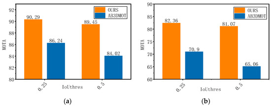
Figure 7.
Comparison of MOTA between our algorithm and the baseline at different IoUthres. (a) shows the tracking accuracy comparison for cars under varying thresholds, whereas (b) illustrates the corresponding results for pedestrians.
It can be observed that under different matching criteria, our algorithm consistently demonstrates superior performance in MOTA (Multi-Object Tracking Accuracy metrics). Under IoU thresholds of 0.25 and 0.5, our algorithm achieves tracking accuracy rates of 90.29 and 89.45 for cars, respectively, outperforming AB3DMOT, which obtains 86.24 and 84.02 under the same settings. Due to their smaller size and greater variability in motion, pedestrians are generally more difficult to track than vehicles. Under an IoU threshold of 0.5, AB3DMOT achieves a tracking accuracy of 65.06 for pedestrians, while our method significantly improves this performance, reaching an accuracy of 81.07. The superior accuracy of our algorithm is attributed to its effective integration of image and point cloud data. Our algorithm inputs both 2D and 3D detection boxes into the tracker. If the detector produces poor 3D detection results in certain frames, resulting in a significant decrease in similarity with the predicted outcomes, the tracker assigns the correct ID to the object based on the 2D detection boxes. The incorporation of multimodal data prevents ID-switching errors caused by failed 3D detections, ultimately enabling our algorithm to achieve superior performance metrics. Figure 8 illustrates the tracking performance for cars in terms of the HOTA metric, comparing our algorithm with AB3DMOT. The results shown in the figure provide additional validation of our analysis and conclusions.
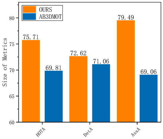
Figure 8.
Tracking performance for cars in terms of the HOTA metric. Our algorithm achieves a higher association accuracy (AssA), which contributes to a higher overall HOTA score.
In Figure 8, the different metrics represent the differences between our method and the baseline algorithms at various stages of tracking. Specifically, HOTA reflects the overall accuracy of detection and tracking; a higher DetA (detection accuracy) indicates better detection accuracy, while a higher AssA (association accuracy) corresponds to higher association accuracy. The AB3DMOT algorithm employs the PointRCNN network during the detection phase, achieving a detection accuracy of 71.06. Although we do not employ a point cloud neural network, our detection accuracy remains slightly higher than that of AB3DMOT. Moreover, due to our use of multi-level data association and a similarity computation method based on multi-sensor data fusion, our association accuracy is significantly higher than that of AB3DMOT. Therefore, our method achieves higher overall tracking accuracy (HOTA) compared to the baseline algorithm.
In addition to AB3DMOT, we further compare the performance of our algorithm on the KITTI validation set with that of other classical and recently proposed tracking methods. The results are presented in Table 1.

Table 1.
Performance of car tracking on the kitti val set using the clear metrics.
In Table 1, the IoU threshold is set to 0.5, which is a commonly used value in metric computation. Our algorithm achieves a MOTA (Multi-Object Tracking Accuracy metrics) of 89.45, a MOTP of 81.87, a FRAG of 26, and an IDS of 11, where MOTA stands for comprehensive tracking performance and FRAG represents the number of trajectory fragments. The experimental results clearly indicate that our algorithm achieves superior performance compared to several well-established tracking algorithms, which demonstrates that our proposed fusion algorithm achieves the desired performance. Naturally, we do not aim for our algorithm to outperform the most advanced multi-object tracking methods in terms of accuracy. Instead, our primary objective is to ensure efficiency without compromising accuracy, thereby making the algorithm more suitable for deployment on low-cost UGV platforms. Overall, the accuracy of our algorithm is comparable to the results reported in the latest published studies. However, by employing a point cloud clustering algorithm to extract 3D features instead of relying on complex neural networks, our algorithm achieves higher efficiency and greater lightweight capability. In the next section, we will provide a detailed comparison of the computational complexity and efficiency between our algorithm and others.
6.3.2. Ablation Studies
As described in Section 4 and Section 5, the proposed framework first conducts 2D object detection using a YOLO model integrated with an SE module, then extracts object point clouds using DBSCN, and ultimately achieves object tracking through multi-level data association. In this subsection, we conduct a sequential analysis of how the SE module, the parameter settings of the DSSCN algorithm, and the multi-level data association module affect the detection and tracking performance. This part of the experiment is also conducted on the KITTI dataset, as its ground-truth annotations can be used for metric computation.
Effect of SE module: Table 2 presents the HOTA metrics of the tracking algorithm using different detection models. Specifically, HOTA reflects the overall tracking performance; DetA, DetRe, and DetPr indicate the detection accuracy, recall, and precision, respectively; while AssA, AssRe, and AssPr denote the association accuracy, recall, and precision, respectively. It can be concluded that incorporating the SE module improves all metrics. The results suggest that the tracking performance could be further improved by integrating more sophisticated modules or by substituting YOLO with a more advanced neural network architecture. However, this is not the primary focus of our work. YOLO offers a favorable balance between accuracy and efficiency, as its end-to-end detection framework achieves faster inference than two-stage detection methods. Therefore, YOLO demonstrates greater advantages when applied to autonomous navigation scenarios with high efficiency requirements.
Table 2.
Performance of car tracking with different detection models.
Effect of DBSCAN parameters: As mentioned in Section 4.3.2, the input parameters of the clustering algorithm include the neighborhood radius and the threshold . Table 3 presents the variations in the evaluation metrics under different values of these two parameters. The evaluated metrics include MOTA, HOTA, MOTP, and DetA. Among them, MOTA and HOTA are used to assess the overall tracking performance, DetA evaluates the algorithm’s ability to correctly detect targets, and MOTP reflects the localization accuracy for the detected objects.
Table 3.
Performance of car tracking with different clustering parameters.
As shown in Table 3, when the neighborhood radius is set to 0.1, the algorithm exhibits a weaker ability to successfully detect objects, resulting in a significant decrease in the DetA metric. The overall tracking performance metrics, MOTA and HOTA, also decline accordingly. However, unlike these metrics, MOTP increases under this parameter setting, indicating that the localization accuracy for successfully detected objects remains unaffected. This indicates that the neighborhood radius should not be set too small. Since points in a point cloud are spatially discrete, an excessively small neighborhood radius may cause a single object to be split into multiple clusters. It is worth noting that when the neighborhood radius is set above 0.3, variations in either parameter have little impact on the final detection and tracking performance.
These results suggest that the proposed algorithm is relatively insensitive to parameter variations. This robustness stems from the spatial distribution differences between the object points and the noisy point clouds. The point cloud roughly extracted based on 2D detection boxes consists of target points, ground points, and points belonging to other objects. While ground points are spatially adjacent to the target points, they are eliminated during the ground filtering stage. In contrast, point clouds from other objects are spatially separated from the target, as shown in Figure 9. Therefore, it is easy to use the clustering algorithm to distinguish them. This fact allows the input parameters of the clustering process to be chosen within a relatively wide range. Such robustness to parameter settings further improves the practical applicability of our method in engineering applications.
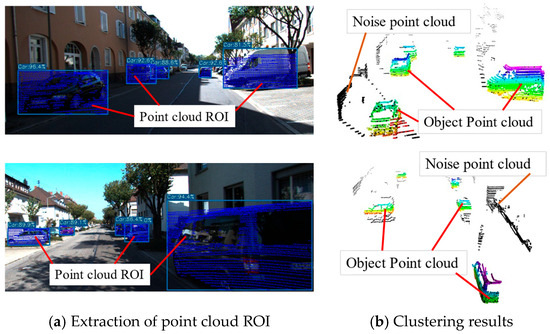
Figure 9.
The point cloud within the detection box and the clustering results. In (a), the blue region within the detection box represents the point cloud ROI, which consists of both the object point clouds and the noise point clouds. In (b), the colored point clouds represent the object point clouds extracted using the clustering algorithm, while the black points correspond to background noise. It can be observed that although the object point clouds and the noise points are enclosed within the same detection box in the 2D image, their positions differ significantly in 3D space.
Effect of multi-level data association: The proposed multi-level data association strategy aims to reduce the influence of detection errors on tracking performance. In the KITTI dataset, such errors are typically caused by mutual occlusions between targets. Therefore, the evaluation metrics in this experiment are calculated using the KITTI 06, 08, 14, and 15 sequences, where vehicle occlusions occur more frequently.
Table 4 summarizes the car tracking results of our method and the comparison approaches on the selected sequences. Method A does not categorize the detection results. Instead, it directly performs data association between detections with confidence scores above 0.1 and existing trajectories using the Hungarian algorithm. Method B, on the other hand, divides the detection results into two groups based on confidence scores. It first associates the high-confidence detections with existing trajectories, and then associates the low-confidence detections with the remaining trajectories. Both Method A and Method B use the similarity function designed in this work for data association, which is a weighted combination of 2D IoU and 3D Mahalanobis distance. Specifically, metrics associated with data association are reported in the table. HOTA and MOTA offer an overall assessment of tracking performance, AssA evaluates the precision of trajectory association, and FRAG indicates the frequency of trajectory breaks resulting from false detections, missed detections, or identity switches.
Table 4.
Performance of car tracking with different data association strategies.
It can be observed that the adoption of multi-level data association improves tracking performance, with a particularly notable reduction in FRAG. While Methods A and B share identical FRAG metrics, our approach lowers this value from 30 to 11, indicating that the designed multi-level data association strategy helps prevent fragmentation of trajectories. During the object detection process, some partially occluded objects have few associated point cloud points, which makes the clustering process difficult to be carred out. As a result, Methods A and B directly discard these objects, since the Mahalanobis distance cannot be computed without clustered point clouds. Such cases cause some trajectories failing to be correctly associated with objects, ultimately leading to an increase in the FRAG value. In our method, the third data association stage is specifically designed to handle such cases. When 3D information is missing, it associates these targets with trajectories using 2D detection results, thereby significantly reducing trajectory fragmentation.
6.3.3. Tracking Performance in Scenes with High Object Density
As we have emphasized several times, the core of this work is to provide an efficient multi-object tracking algorithm that can be deployed on low-cost devices. Therefore, we abandon 3D point cloud neural networks and instead employ a 2D image-based neural network combined with a clustering algorithm for 3D information extraction. Since 2D object detection is the first step of the algorithm, it largely determines the final tracking performance. While 2D object detection offers efficiency advantages over its 3D counterpart due to the reduced dimensionality, it also constrains our algorithm from reaching the performance of state-of-the-art detection and tracking approaches in terms of accuracy. In this section, we analyze the detection and tracking performance of our algorithm in environments with high target density, which helps assess its limitations and evaluate its robustness for practical applications.
Table 5 presents the pedestrian tracking performance metrics of our algorithm on two KITTI sequences with high object density (sequences 13 and 16). The specific scenarios corresponding to the two sequences are shown in Figure 10. It can be observed that each scene contains a large number of pedestrians. Columns 2 to 3 of the table present the performance metrics of our method on sequences 13 and 16, respectively, while the last column provides the aggregated metrics across all 11 validation sequences. In sequences 13 and 16, the object detection performance is relatively poor, resulting in lower DetA values. Consequently, the overall tracking metric MOTA is also relatively low due to the impact of detection results.
Table 5.
Performance of pedestrian tracking in in sequences with high object density.
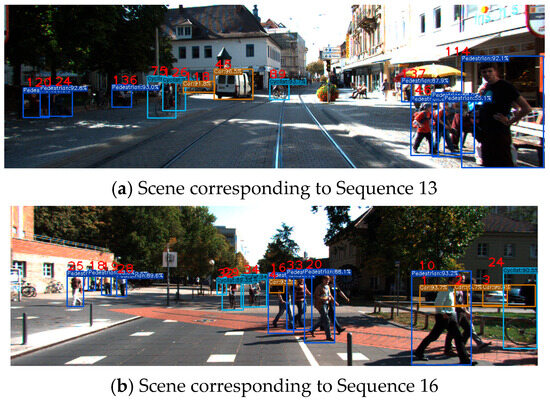
Figure 10.
The scenes with high target density selected from the three KITTI datasets. These two sequences contain dense distributions of pedestrians, cyclists, and vehicles, which are enclosed by dark blue, light blue, and orange bounding boxes, respectively, during the 2D object detection stage.
It is noteworthy that, despite the relatively poor detection performance in these two scenarios, the AssA values remain high, indicating that the accuracy of data association is not significantly affected by detection errors. In Figure 11, we present three frames of detection and tracking results, along with the corresponding trajectories in the point cloud coordinate system. In frame 496, the object 121 is occluded, resulting in a relatively small number of corresponding point cloud points. Under such circumstances, it is difficult to detect the target in 3D space. However, our multi-level data association strategy leverages 2D image data to maintain the target’s ID, thereby preventing trajectory fragmentation. Similarly, the IDs of distant targets remain unchanged under our algorithm, and their corresponding trajectories consistently retain the same color.
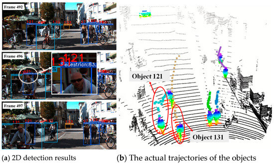
Figure 11.
Tracking visualization on the KITTI dataset. (a) presents the detection results of three frames of images. In frame 496, object 121 is occluded by object 131. (b) shows the trajectories of the objects, where the cyan and brown trajectories correspond to targets No. 121 and No. 131, respectively. The trajectories in other colors correspond to the estimated trajectories of other objects. Our multi-level data association strategy ensures that the ID of object 131 remains unchanged after occlusion, and its corresponding trajectory remains continuous without fragmentation.
6.4. Results on a Real UGV Platform
6.4.1. Comparison of Efficiency
As the runtime of an object tracking algorithm is largely influenced by the detection process, this sub-section focuses on evaluating the efficiency of our detection method. To accurately demonstrate the practical value of our algorithm, we conducted efficiency evaluation experiments on a real vehicle platform, where the industrial computer was not equipped with a GPU. Before deploying the algorithm, we needed to convert the model, as the runtime efficiency of different model formats varies significantly in a CPU environment.
Figure 12 presents the detection time per frame of our algorithm on an Intel i5-12600 CPU when using different neural network models. The total runtime consists of both the 2D object detection process and the clustering-based 3D information extraction. The three curves in the figure represent the 3D object detection time corresponding to the PyTorch model, ONNX model, and OpenVINO model, respectively. The PyTorch model (PyTorch 2.4.1) is directly obtained as the output of the training process. It is first converted to the ONNX format and then further optimized into the OpenVINO format, which is specifically tailored for Intel processors. It can be observed that the OpenVINO model demonstrates the highest inference efficiency on our vehicle platform, owing to its optimization and specific design for Intel CPUs. Therefore, improving algorithm efficiency does not necessarily require modifying the algorithm or neural network structure. Selecting an appropriate inference framework based on the specific hardware can enhance the algorithm’s real-world performance.
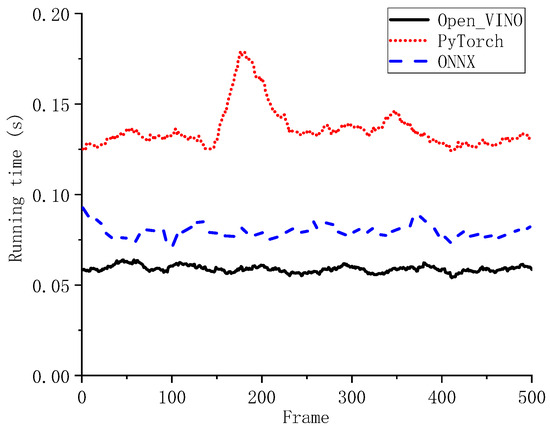
Figure 12.
Comparison of the running time of our detector when using models in various formats.
To demonstrate that our algorithm is not dependent on specific hardware, we conducted efficiency tests using the ONNX-format model on different hardware platforms, including different LiDAR sensors and different CPUs. In Table 6, the point cloud and image data corresponding to the 64-line LiDAR are from the KITTI dataset, while the data for the 32-line and 16-line LiDARs are collected from our own robotic platform. Since our image data differ from those in the KITTI dataset, the corresponding 2D detection times also vary significantly. However, in all experiments, the time consumed by point cloud clustering is far less than that of 2D object detection. Moreover, as the number of LiDAR channels decreases, the clustering time further reduces. As shown in Table 7, when our algorithm is deployed on an Intel i7-9750H CPU released in 2019, the per-detection time increases slightly, but it still only requires approximately 100 ms. Therefore, we can conclude that the efficiency of our method is minimally affected by the hardware. Even when using a 64-line LiDAR and a relatively low-performance CPU such as the i7-9750H, our method still maintains high efficiency.
Table 6.
Running time of our detector on i5-12600 CPU with different LiDAR sensors.
Table 7.
Running time of our detector on i7-9750H CPU with different LiDAR sensors.
To further demonstrate the efficiency advantage of our algorithm, we compared the runtime of our detection algorithm with that of other methods. Table 8 summarizes the operating environments and the detection time per frame for different algorithms.
Table 8.
Comparison of the running time of our detector and commonly used detectors.
The data in Table 8 clearly demonstrates the substantial efficiency advantage of our algorithm. In the same CPU environment, PointGNN takes an average of 1.43 s to perform object detection on a single frame, whereas our algorithm requires only 0.059 s. The other three algorithms in the table, despite utilizing GPUs for inference, still fall short of the runtime efficiency achieved by our algorithm. The R-GCN algorithm requires 0.26 s for object detection using a 1080Ti GPU. Undoubtedly, it would take even longer if deployed on our vehicle platform, which is unacceptable for the real-time autonomous navigation task. In contrast, our algorithm can run efficiently on devices with limited computational resources, making it highly valuable for practical applications.
6.4.2. Detection Results Using a 32-Line LIDAR
The strengths of our algorithm lie not only in its computational efficiency but also in its compatibility with 32-line LiDAR systems. Therefore, in this work, we not only calculate metrics on public datasets but also conduct experiments using a real UGV platform in real campus environments. The UGV platform is equipped with a monocular camera and a 32-line LiDAR. Figure 13 and Figure 14 illustrate the object labels in the image and their corresponding trajectories in 3D space, respectively.
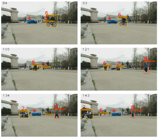
Figure 13.
Visual display of detection and tracking results in real scenarios.
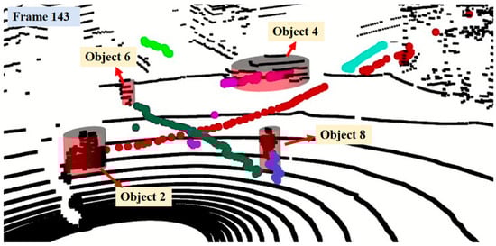
Figure 14.
The trajectory of the objects generated by our algorithm in a real-world scenario. The curves formed by points of different colors represent the trajectories corresponding to different objects. Certain trajectories in Figure 11 correspond to objects that are not present in Figure 10 but do appear in other frames of the sequence.
As shown in Figure 13, the 84th frame image includes the cyclist labeled as No. 2, the car labeled as No. 4, and the cyclist labeled as No. 6. However, mutual occlusion occurs among these objects in frames 93, 105, 121, and 134, resulting in the detector’s inability to accurately identify individual objects. In frame 143, when the detector re-detects these objects, our tracking algorithm correctly restores their respective labels. Figure 14 displays the point cloud data for the 143rd frame. The black points depict the raw LiDAR point cloud, serving as the detector’s input. The cylindrical bounding boxes represent the detector’s output, enclosing the detected object point clouds. The lines formed by points of different colors illustrate the historical trajectories of the tracked objects, where distinct colors correspond to different object labels. It can be observed that occlusion causes the trajectories not to be strictly continuous. Nevertheless, the trajectory of each object maintains a consistent color, demonstrating that occlusion does not cause trajectory fragmentation. Thus, this experiment validates the robustness of our algorithm in real-world scenarios.
7. Conclusions
In this study, we presented an efficient 3D object detection and tracking framework tailored for resource-constrained UGV platforms. By combining an image-based 2D detector with data fusion and unsupervised learning techniques, our method effectively extracts and isolates object point clouds without relying on computationally intensive neural networks. The integration of both 2D and 3D information during the tracking phase improves association accuracy and reduces the impact of detection errors. Experimental results on the KITTI benchmark demonstrate that our approach achieves notable computational efficiency while maintaining high detection accuracy. Additionally, real-world deployment tests validate the practicality and robustness of our method on low-cost vehicle systems, confirming its suitability for embedded applications with limited processing capabilities.
Author Contributions
Conceptualization, X.Y., W.F. and J.Y.; Methodology, X.Y., A.H., J.L. and J.Y.; Software, A.H. and J.L.; Validation, J.L. and J.G.; Investigation, X.Y.; Data curation, J.G.; Writing—original draft, X.Y. and A.H.; Supervision, W.F.; Project administration, W.F.; Funding acquisition, J.Y. All authors have read and agreed to the published version of the manuscript.
Funding
This work was funded by the Industrial Key Research and Development Projects of Shaanxi Province, grant number 2024CY2-GIHX-91, and the Practice and Innovation Funds for Graduate Students of Northwestern Polytechnical University, grant number PF2025067.
Data Availability Statement
The original contributions presented in this study are included in the article. Further inquiries can be directed to the corresponding author.
Conflicts of Interest
The authors declare no conflict of interest.
References
- Nahavandi, S.; Alizadehsani, R.; Nahavandi, D.; Mohamed, S.; Mohajer, N.; Rokonuzzaman, M.; Hossain, I. A comprehensive review on autonomous navigation. ACM Comput. Surv. 2025, 57, 234. [Google Scholar] [CrossRef]
- Tang, W.; Huang, A.; Liu, E.; Wu, J.; Zhang, R. A Reliable Robot Localization Method Using LiDAR and GNSS Fusion Based on a Two-Step Particle Adjustment Strategy. IEEE Sens. J. 2024, 24, 37846–37858. [Google Scholar]
- Hung, N.; Rego, F.; Quintas, J.; Cruz, J.; Jacinto, M.; Souto, D.; Potes, A.; Sebastiao, L.; Pascoal, A. A review of path following control strategies for autonomous robotic vehicles: Theory, simulations, and experiments. J. Field Robot. 2023, 40, 747–779. [Google Scholar] [CrossRef]
- Xu, G.; Khan, A.S.; Moshayedi, A.J.; Zhang, X.; Yang, S. The object detection, perspective and obstacles in robotic: A review. EAI Endorsed Trans. AI Robot. 2022, 1, e13. [Google Scholar] [CrossRef]
- Qi, W.; Xu, X.; Qian, K.; Schuller, B.W.; Fortino, G.; Aliverti, A. A Review of AIoT-Based Human Activity Recognition: From Application to Technique. IEEE J. Biomed. Health Inform. 2025, 29, 2425–2438. [Google Scholar] [CrossRef] [PubMed]
- Ravindran, R.; Santora, M.J.; Jamali, M.M. Multi-object detection and tracking, based on DNN, for autonomous vehicles: A review. IEEE Sens. J. 2020, 21, 5668–5677. [Google Scholar] [CrossRef]
- Bewley, A.; Ge, Z.; Ott, L.; Ramos, F.; Upcroft, B. Simple online and realtime tracking. In Proceedings of the 2016 IEEE International Conference on Image Processing (ICIP), Phoenix, AZ, USA, 25–28 September 2016. [Google Scholar]
- Malagoli, E.; Di Persio, L. 2D Object Detection: A Survey. Mathematics 2025, 13, 893. [Google Scholar] [CrossRef]
- An, P.; Zhu, D.; Quan, S.; Ding, J.; Ma, J.; Yang, Y.; Liu, Q. ESC-Net: Alleviating Triple Sparsity on 3D LiDAR Point Clouds for Extreme Sparse Scene Completion. IEEE Trans. Multimed. 2024, 26, 6799–6810. [Google Scholar]
- Milioto, A.; Vizzo, I.; Behley, J.; Stachniss, C. RangeNet++: Fast and accurate LiDAR semantic segmentation. In Proceedings of the 2019 IEEE/RSJ International Conference on Intelligent Robots and Systems (IROS), Macau, China, 3–8 November 2019. [Google Scholar]
- Meyer, G.P.; Laddha, A.; Kee, E.; Vallespi-Gonzalez, C.; Wellington, C.K. Lasernet: An efficient probabilistic 3d object detector for autonomous driving. In Proceedings of the IEEE/CVF Conference on Computer Vision and Pattern Recognition, Long Beach, CA, USA, 16–20 June 2019. [Google Scholar]
- Chen, X.; Ma, H.; Wan, J.; Li, B.; Xia, T. Multi-view 3d object detection network for autonomous driving. In Proceedings of the IEEE Conference on Computer Vision and Pattern Recognition, Honolulu, HI, USA, 21–26 July 2017. [Google Scholar]
- Ye, M.; Xu, S.; Cao, T. Hvnet: Hybrid voxel network for lidar based 3d object detection. In Proceedings of the IEEE/CVF Conference on Computer Vision and Pattern Recognition, Virtual, 16–18 June 2020. [Google Scholar]
- Lang, A.H.; Vora, S.; Caesar, H.; Zhou, L.; Yang, J.; Beijbom, O. PointPillars: Fast encoders for object detection from point clouds. In Proceedings of the IEEE/CVF Conference on Computer Vision and Pattern Recognition, Long Beach, CA, USA, 16–20 June 2019. [Google Scholar]
- Zhou, Y.; Tuzel, O. Voxelnet: End-to-end learning for point cloud based 3d object detection. In Proceedings of the IEEE Conference on Computer Vision and Pattern Recognition, Salt Lake City, UT, USA, 19–21 June 2018. [Google Scholar]
- Qi, C.R.; Su, H.; Mo, K.; Guibas, L.J. Pointnet: Deep learning on point sets for 3d classification and segmentation. In Proceedings of the IEEE Conference on Computer Vision and Pattern Recognition, Honolulu, HI, USA, 21–26 July 2017. [Google Scholar]
- Zhao, H.; Jiang, L.; Jia, J.; Torr, P.H.; Koltun, V. Point transformer. In Proceedings of the IEEE/CVF International Conference on Computer Vision, Virtual, 11–17 October 2021. [Google Scholar]
- Weng, X.; Wang, J.; Held, D.; Kitani, K. 3D Multi-Object Tracking: A Baseline and New Evaluation Metrics. In Proceedings of the IEEE/RSJ International Conference on Intelligent Robots and Systems (IROS), Las Vegas, NV, USA, 25–29 October 2020. [Google Scholar]
- Cheng, X.; Zhou, J.; Liu, P.; Zhao, X.; Wang, H. 3D vehicle object tracking algorithm based on bounding box similarity measurement. IEEE Trans. Intell. Transp. Syst. 2023, 24, 15844–15854. [Google Scholar] [CrossRef]
- Fu, Z.; Shang, H.; Song, L.; Li, Z.; Chen, C. Camera-LiDAR Fusion Based Three-Stages Data Association Framework for 3D Multi-Object Tracking. In Proceedings of the 2nd International Conference on Networking Systems of AI (INSAI), Shanghai, China, 14–15 October 2022. [Google Scholar]
- Zhang, Y.; Sun, P.; Jiang, Y.; Yu, D.; Weng, F. Bytetrack: Multi-object tracking by associating every detection box. In Proceedings of the European Conference on Computer Vision, Tel Aviv, Israel, 23–27 October 2022. [Google Scholar]
- Zhan, Y.; Wang, X.-H.; Ye, X.; Zhang, W.; Lu, J.; Tan, X.; Ding, E.; Sun, P.; Wang, J. ByteTrackV2: 2D and 3D multi-object tracking by associating every detection box. arXiv 2023, arXiv:2303.15334. [Google Scholar]
- Shi, G.; Li, R.; Ma, C. Pillarnet: Real-time and high-performance pillar-based 3d object detection. In Proceedings of the European Conference on Computer Vision, Tel Aviv, Israel, 23–27 October 2022. [Google Scholar]
- Su, H.; Schmirander, Y.; Li, Z.; Zhou, X.; Ferrigno, G.; De Momi, E. Bilateral Teleoperation Control of a Redundant Manipulator with an RCM Kinematic Constraint. In Proceedings of the 2020 IEEE International Conference on Robotics and Automation (ICRA), Paris, France, 31 May–31 August 2020. [Google Scholar]
- Li, B.; Zhang, T.; Xia, T. Vehicle detection from 3d lidar using fully convolutional network. arXiv 2016, arXiv:1608.07916. [Google Scholar] [CrossRef]
- Beltran, J.; Guindel, C.; Moreno, F.M.; Cruzado, D.; Garcia, F.; De La Escalera, A. BirdNet: A 3D object detection framework from LiDAR information. In Proceedings of the 21st International Conference on Intelligent Transportation Systems, Maui, HI, USA, 4–7 November 2018. [Google Scholar]
- Yan, Y.; Mao, Y.; Li, B. SECOND: Sparsely Embedded Convolutional Detection. Sensors 2018, 18, 3337. [Google Scholar] [CrossRef] [PubMed]
- Wu, Y.; Wang, Y.; Zhang, S.; Ogai, H. Deep 3D object detection networks using LiDAR data: A review. IEEE Sens. J. 2020, 21, 1152–1171. [Google Scholar] [CrossRef]
- Shi, S.; Wang, X.; Li, H. PointRCNN: 3D object proposal generation and detection from point cloud. In Proceedings of the IEEE/CVF Conference on Computer Vision and Pattern Recognition, Long Beach, CA, USA, 16–20 June 2019. [Google Scholar]
- Qi, C.R.; Liu, W.; Wu, C.; Su, H.; Guibas, L.J. Frustum PointNets for 3D Object Detection from RGB-D Data. In Proceedings of the IEEE/CVF Conference on Computer Vision and Pattern Recognition, Salt Lake City, UT, USA, 18–20 June 2018. [Google Scholar]
- Sindagi, V.A.; Zhou, Y.; Tuzel, O. Mvx-net: Multimodal voxelnet for 3d object detection. In Proceedings of the International Conference on Robotics and Automation (ICRA), Montreal, QC, Canada, 20–24 May 2019. [Google Scholar]
- Pang, S.; Morris, D.; Radha, H. CLOCs: Camera-LiDAR object candidates fusion for 3D object detection. In Proceedings of the IEEE/RSJ International Conference on Intelligent Robots and Systems, Las Vegas, NV, USA, 25–29 October 2020. [Google Scholar]
- Pang, S.; Morris, D.; Radha, H. Fast-CLOCs: Fast camera-LiDAR object candidates fusion for 3D object detection. In Proceedings of the IEEE/CVF Winter Conference on Applications of Computer Vision, Waikoloa, HI, USA, 4–8 January 2022. [Google Scholar]
- Yu, Z.; Qiu, B.; Khong, A.W.H. ViKIENet: Towards Efficient 3D Object Detection with Virtual Key Instance Enhanced Network. In Proceedings of the 2025 IEEE/CVF Conference on Computer Vision and Pattern Recognition (CVPR), Nashville, TN, USA, 16–20 June 2025. [Google Scholar]
- Hoang, H.; Bui, D.; Yoo, M. TSSTDet: Transformation-Based 3-D Object Detection via a Spatial Shape Transformer. IEEE Sens. J. 2024, 24, 7126–7139. [Google Scholar] [CrossRef]
- Hu, H.-N.; Yang, Y.-H.; Fischer, T.; Darrell, T.; Yu, F.; Sun, M. Monocular quasi-dense 3d object tracking. IEEE Trans. Pattern Anal. Mach. Intell. 2022, 45, 1992–2008. [Google Scholar] [CrossRef] [PubMed]
- Bae, S.H.; Yoon, K.J. Robust online multi-object tracking based on tracklet confidence and online discriminative appearance learning. In Proceedings of the IEEE Conference on Computer Vision and Pattern Recognition, Columbus, OH, USA, 24–27 June 2014. [Google Scholar]
- Sander, J.; Ester, M.; Kriegel, H.P.; Xu, X. Density-Based Clustering in Spatial Databases: The Algorithm GDBSCAN and Its Applications. Data Min. Knowl. Discov. 1998, 2, 169–194. [Google Scholar] [CrossRef]
- Yin, T.; Zhou, X.; Krahenbuhl, P. Center-based 3D Object Detection and Tracking. In Proceedings of the IEEE/CVF Conference on Computer Vision and Pattern Recognition (CVPR), Nashville, TN, USA, 19–25 June 2021. [Google Scholar]
- Luiten, J.; Osep, A.; Dendorfer, P.; Torr, P.; Geiger, A.; Leal-Taixé, L.; Leibe, B. Hota: A higher order metric for evaluating multi-object tracking. Int. J. Comput. Vis. 2021, 129, 548–578. [Google Scholar] [CrossRef] [PubMed]
- Zhang, W.; Zhou, H.; Sun, S.; Wang, Z.; Shi, J.; Chen, C.L. Robust multi-modality multi-object tracking. In Proceedings of the IEEE/CVF International Conference on Computer Vision (ICCV), Seoul, Republic of Korea, 27 October–2 November 2019. [Google Scholar]
- Baser, E.; Balasubramanian, V.; Bhattacharyya, P.; Czarnecki, K. FANTrack: 3D Multi-Object Tracking with Feature Association Network. In Proceedings of the 2019 IEEE Intelligent Vehicles Symposium (IV), Paris, France, 9–12 June 2019. [Google Scholar]
- Wang, L.; Zhang, X.; Qin, W.; Li, X.; Gao, J.; Yang, L.; Li, Z.; Li, J.; Zhu, L.; Wang, H.; et al. Camo-mot: Combined appearance-motion optimization for 3d multi-object tracking with camera-lidar fusion. IEEE Trans. Intell. Transp. Syst. 2023, 24, 11981–11996. [Google Scholar] [CrossRef]
- Weng, X.; Wang, Y.; Man, Y.; Kitani, K.M. GNN3DMOT: Graph neural network for 3d multi-object tracking with 2d-3d multi-feature learning. In Proceedings of the IEEE/CVF Conference on Computer Vision and Pattern Recognition (CVPR), Virtual, 16–18 June 2020. [Google Scholar]
- Zhai, G.; Kong, X.; Cui, J.; Liu, Y.; Yang, Z. Flowmot: 3d multi-object tracking by scene flow association. arXiv 2021, arXiv:2012.07541v3. [Google Scholar]
- Shi, W.; Rajkumar, R. Point-gnn: Graph neural network for 3d object detection in a point cloud. In Proceedings of the IEEE/CVF Conference on Computer Vision and Pattern Recognition, Virtual, 16–18 June 2020. [Google Scholar]
- Degraeve, V.; Vandewiele, G.; Ongenae, F.; Van Hoecke, S. R-GCN: The R could stand for random. arXiv 2022, arXiv:2203.02424. [Google Scholar] [CrossRef]
- Chen, Y.; Liu, S.; Shen, X.; Jia, J. Fast point r-cnn. In Proceedings of the IEEE/CVF International Conference on Computer Vision (ICCV), Seoul, Republic of Korea, 27 October–2 November 2019. [Google Scholar]
Disclaimer/Publisher’s Note: The statements, opinions and data contained in all publications are solely those of the individual author(s) and contributor(s) and not of MDPI and/or the editor(s). MDPI and/or the editor(s) disclaim responsibility for any injury to people or property resulting from any ideas, methods, instructions or products referred to in the content. |
© 2025 by the authors. Licensee MDPI, Basel, Switzerland. This article is an open access article distributed under the terms and conditions of the Creative Commons Attribution (CC BY) license (https://creativecommons.org/licenses/by/4.0/).