MobileAmcT: A Lightweight Mobile Automatic Modulation Classification Transformer in Drone Communication Systems

Abstract

With the rapid advancement of wireless communication technology, automatic modulation classification (AMC) plays a crucial role in drone communication systems, ensuring reliable and efficient communication in various non-cooperative environments. Deep learning technology has demonstrated significant advantages in the field of AMC, effectively and accurately extracting and classifying modulation signal features. However, existing deep learning models often have high computational costs, making them difficult to deploy on resource-constrained drone communication devices. To address this issue, this study proposes a lightweight Mobile Automatic Modulation Classification Transformer (MobileAmcT). This model combines the advantages of lightweight convolutional neural networks and efficient Transformer modules, incorporating the Token and Channel Conv (TCC) module and the EfficientShuffleFormer module to enhance the accuracy and efficiency of the automatic modulation classification task. The TCC module, based on the MetaFormer architecture, integrates lightweight convolution and channel attention mechanisms, significantly improving local feature extraction efficiency. Additionally, the proposed EfficientShuffleFormer innovatively improves the traditional Transformer architecture by adopting Efficient Additive Attention and a novel ShuffleConvMLP feedforward network, effectively enhancing the global feature representation and fusion capabilities of the model. Experimental results on the RadioML2016.10a dataset show that compared to MobileNet-V2 (CNN-based) and MobileViT-XS (ViT-based), MobileAmcT reduces the parameter count by 74% and 65%, respectively, and improves classification accuracy by 1.7% and 1.09% under different SNR conditions, achieving an accuracy of 62.93%. This indicates that MobileAmcT can maintain high classification accuracy while significantly reducing the parameter count and computational complexity, clearly outperforming existing state-of-the-art AMC methods and other lightweight deep learning models.

1. Introduction

Automatic modulation classification (AMC) can automatically identify the modulation types of radio signals transmitted over unknown channels that are affected by fading and noise. It is used to distinguish drone signals and identify interference signals, enabling intelligent spectrum monitoring and management for drone communication systems [1]. AMC can also monitor spectrum usage in real-time, helping drone communication systems switch flexibly between different spectrum resources, thus improving spectrum utilization [2]. Furthermore, by accurately identifying modulation types, AMC improves data transmission rates and output signal-to-noise ratios, ensuring the effectiveness and reliability of drone communication systems [3].

Traditional AMC methods are typically divided into two categories: likelihood-based (LB) and feature-based (FB) methods [4]. Likelihood-based AMC methods utilize Bayesian criteria to construct likelihood ratio tests, calculating the likelihood probabilities of received signals under various modulation types and making decisions by comparing the likelihood ratios with thresholds. Examples include maximum likelihood ratio tests (MLRT), generalized likelihood ratio tests (GLRT), and sequential likelihood ratio tests (SLRT) [5]. Although LB methods are optimal in the Bayesian sense, they have high computational complexity, are sensitive to noise and interference, and can be unstable in complex electromagnetic environments [6]. Feature-based AMC methods, on the other hand, use manually designed features such as cyclostationary features, higher-order cumulants, constellation diagrams, and cyclic spectra [7,8,9], and classify these features using classifiers [10]. Manually designed features are usually based on an understanding and experience of signal modulation types, while classifiers are selected and optimized according to different application requirements and metrics. Examples of classifiers include support vector machines (SVM), k-nearest neighbors (KNN), and artificial neural networks (ANN). While FB methods have lower computational complexity, they are highly dependent on the design of signal features and the choice of classifiers.

In recent years, deep learning (DL) technology has made significant advancements in fields such as natural language processing and image recognition and has been successfully applied to wireless communications [11]. In the domain of automatic modulation classification (AMC), traditional LB and FB methods, despite their achievements, exhibit instability in handling complex and dynamic electromagnetic environments. These methods also face challenges related to the subjectivity of feature design and the dependence on classifiers. In contrast, deep learning learns the non-linear mapping from raw input signals to actual outputs in an end-to-end manner [12], eliminating the need for manually extracted features [13]. This capability allows DL models to automatically learn and adapt to complex signal patterns and environmental changes, thereby demonstrating overwhelming advantages in performance and robustness.

Deep learning model architectures, such as convolutional neural networks (CNN), can effectively utilize the spatial information of signals [14,15]. In reference [16], a CNN consisting of three fully connected layers and three convolutional layers was designed. This CNN achieved automatic modulation classification in an additive white Gaussian noise (AWGN) model by learning deep features from sample data. In reference [17], a short-time discrete Fourier transform was used to convert one-dimensional radio signals into time-frequency images, and a denoising method, SCNN2, was introduced by adding a Gaussian filter to reduce noise. Long Short-Term Memory networks (LSTM) specialize in capturing the temporal information of signals [18,19]. For example, Zhang et al. [20] proposed a new Automatic Modulation Recognition (AMR) method based on Recurrent Neural Networks (RNN), which directly uses raw signal data, thus eliminating the need for manual feature extraction. This method employs two layers of Gated Recurrent Units (GRU) to achieve better recognition accuracy. To fully leverage the local feature extraction capability of CNNs and the temporal modeling capability of RNNs, DL-AMR also incorporates several hybrid networks combining CNN and RNN. Reference [21] effectively extracts features from both time and spatial dimensions by combining one-dimensional (1D) convolution, two-dimensional (2D) convolution, and LSTM layers, with a particular focus on handling individual and combined features of in-phase/quadrature (I/Q) symbols of modulation data. Reference [22] proposed a dual-stream structure based on CNN-LSTM, focusing on the spatio-temporal properties of raw complex time-domain signals. This structure uses CNNs to extract spatial features and LSTMs to process temporal sequence data, simultaneously considering the interactions between different features. Graph Convolutional Networks (GCN) can utilize the topological structure information between signals, capturing their correlations and feature distributions more accurately, thus making the model more sensitive to the structural distribution of data [23]. Tonchev et al. [24] proposed a GCN-based AMC method that includes attention modules and I/Q channel fusion modules, formalizing the multi-level graph structure of modulation signals in the signal domain. Transformers, incorporating self-attention mechanisms, can effectively capture global correlations and long-range dependencies within signals [25], making the recognition of signal modulation types more accurate and reliable. For example, Kong et al. [26] introduced a Transformer-based CTDNN structure, which captures local signal features through a wide and deep convolutional design and extracts global features with a three-layer self-attention module within the Transformer. Reference [27] proposed a Transformer-based FEA-T structure, employing a frame embedding module and optimizing the optimal frame length, while designing dual-branch gated linear units for the Transformer’s feedforward network. Consequently, deep learning techniques are gradually replacing traditional AMC methods, becoming powerful tools for addressing automatic modulation classification problems in wireless communications.

However, the aforementioned studies primarily focus on comparing classification accuracy, paying less attention to crucial aspects of wireless communication, such as parameter efficiency, computational workload, and complexity. In the field of wireless communications, there is an urgent need for lightweight devices, which are widely used in IoT devices, mobile terminals, and sensor nodes. These devices are often constrained by size and power consumption, requiring them to operate in resource-limited environments with significant restrictions on storage space and computational capacity. Despite the outstanding performance of deep neural networks in various fields, their large number of parameters and high computational complexity limit their deployment on lightweight devices. Consequently, finding efficient models and algorithms suitable for lightweight devices has become a pressing task in the field of wireless communications. While some lightweight network structures, such as SqueezeNet [28], MobileNet [29], ShuffleNet [30], Mobileformer [31], and MobileViT [32], have been developed in the field of image processing, they are not specifically designed for handling radio tasks. In other words, directly applying these deep learning models to AMC tasks without sacrificing performance is quite challenging.

Simultaneously, although CNN-based models excel in local feature extraction, their limited receptive field makes it difficult to capture long-range information, potentially leading to insufficient feature extraction and affecting classification results. In contrast, Transformer-based models demonstrate superior performance in global modeling, but their self-attention mechanism’s quadratic complexity is closely related to the input size, resulting in a high computational burden [33,34]. To address these issues, this study proposes a lightweight Mobile AMC Transformer (MobileAmcT) specifically designed for AMC tasks. The MobileAmcT model combines lightweight convolutional neural networks with efficient Transformer modules, effectively extracting modulation features from I/Q signals through continuous model training and weight optimization. Experiments conducted on the public dataset RadioML 2016.10a [35] demonstrate that MobileAmcT outperforms a series of state-of-the-art methods in terms of classification accuracy, parameter count, and computational complexity. Additionally, a series of ablation experiments were conducted to verify the effectiveness and importance of each module in the MobileAmcT model for AMC tasks. The main contributions of this study are as follows:

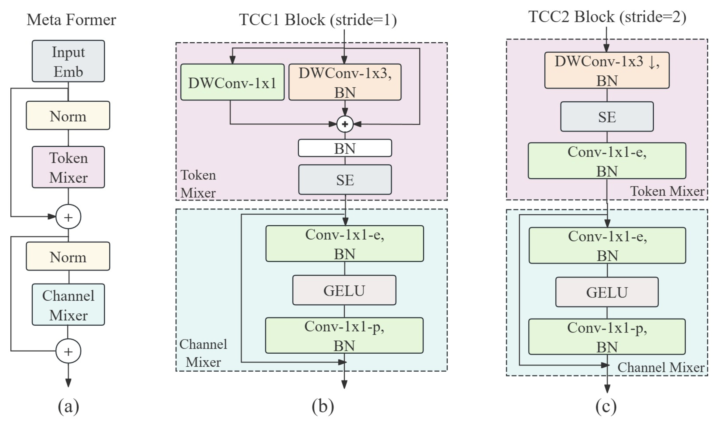
• Proposed TCC1 and TCC2 Modules: In the MobileAmcT model, we have proposed two novel Token and Channel Conv (TCC) modules, TCC1 and TCC2, designed to efficiently capture local features of signals at different levels. These modules are based on the MetaFormer [36] general architecture, integrating the concepts of Token Mixer and Channel Mixer. By combining lightweight convolution and channel attention mechanisms, the TCC modules are structured uniquely to significantly enhance the efficiency and accuracy of local feature extraction while maintaining the model’s lightweight nature.
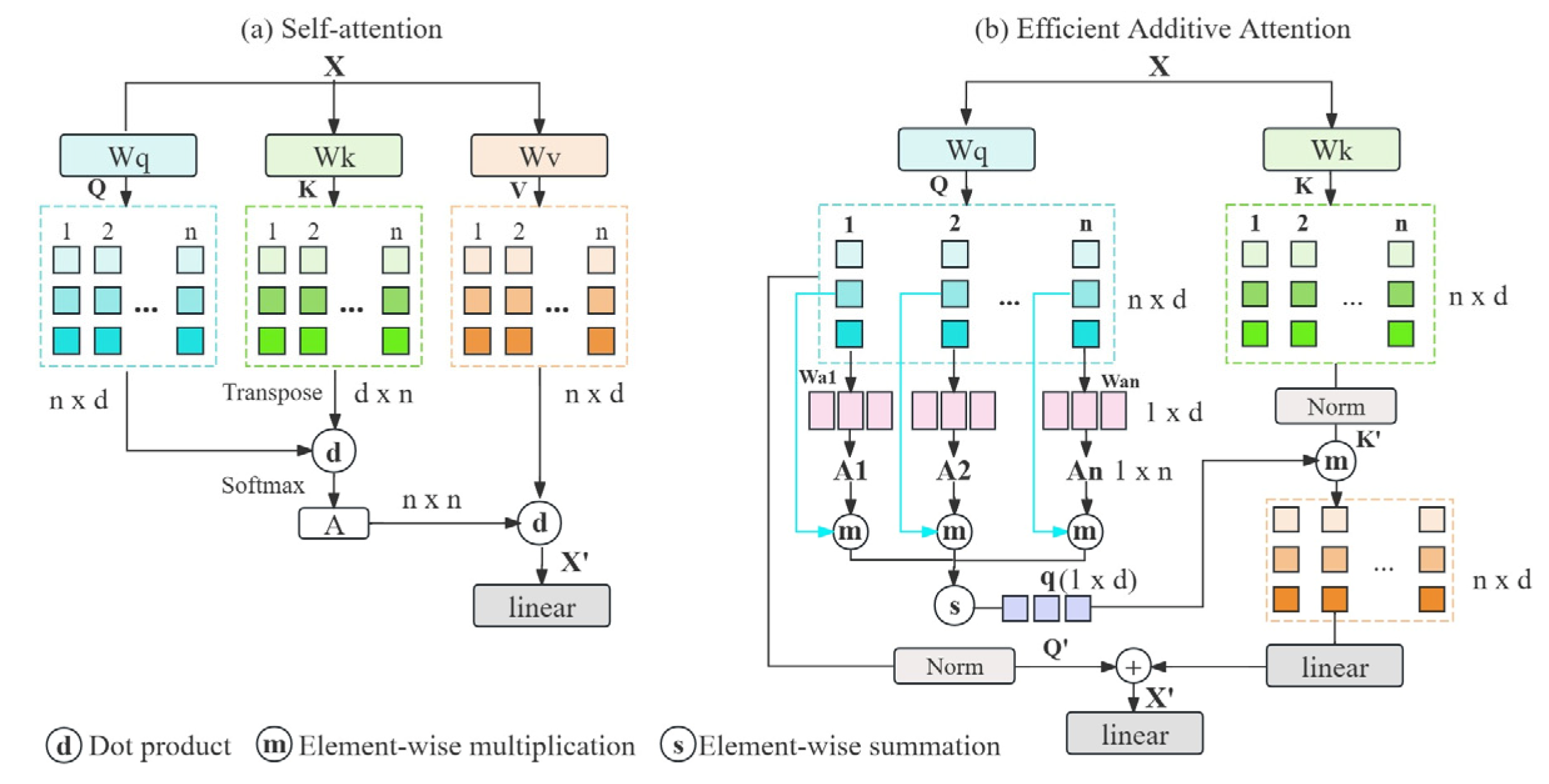
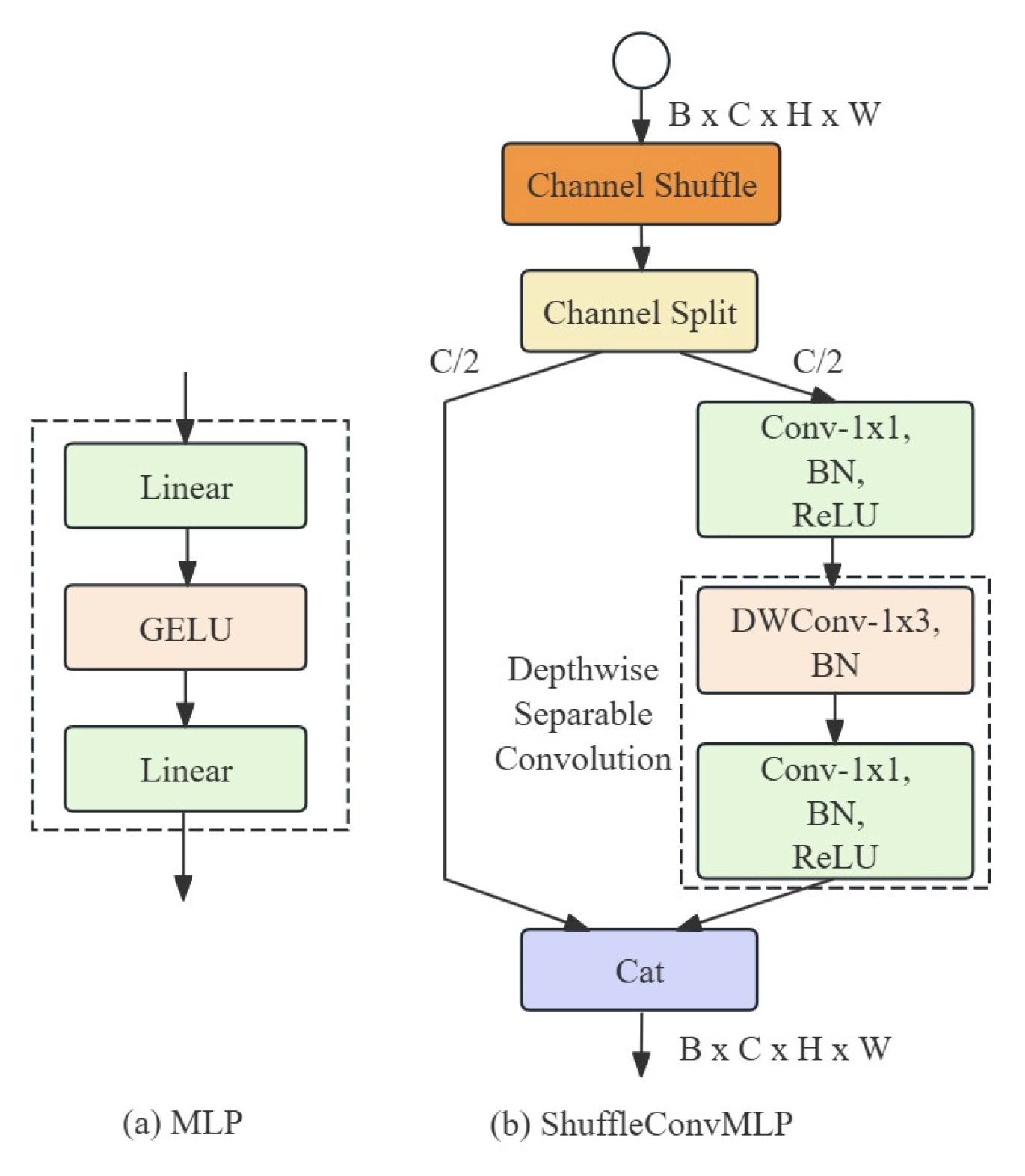
• Innovative EfficientShuffleFormer Module: The EfficientShuffleFormer module in the MobileAmcT model combines Efficient Additive Attention and ShuffleConvMLP to provide efficient global feature representation and fusion capabilities while keeping the model lightweight. Efficient Additive Attention reduces computational complexity by replacing traditional matrix multiplication with element-wise multiplication. ShuffleConvMLP utilizes channel shuffling and depthwise separable convolution techniques to enhance the model’s ability to handle diverse features and capture fine-grained information, thereby improving the efficiency of the feedforward network.
• Enhanced Classification Accuracy and Computational Efficiency: Extensive experiments on the public RadioML2016.10a dataset validate the superior performance of the MobileAmcT model. Compared to existing representative methods, MobileAmcT exhibits high classification accuracy across different SNR environments while significantly reducing the model’s parameter count and computational requirements. The parameters were reduced by up to 82.5%, and classification accuracy was improved by up to 13.6%. Additionally, through ablation experiments, this study systematically evaluates the critical impact and innovative value of core components such as the TCC modules and EfficientShuffleFormer on the overall performance of AMC tasks, showcasing the model’s potential for applications in resource-constrained environments.

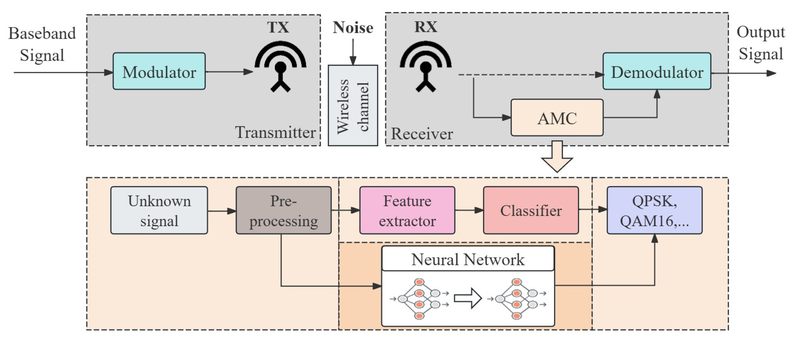
2. AMC System Architecture and Signal Model

2.1. AMC System Architecture

The framework of the AMC system is illustrated in Figure 1. In a non-cooperative communication scenario, the modulator converts the input signals into a form suitable for wireless transmission, which is then transmitted by the transmitter. Due to fading and noise interference in the channel, the receiver cannot directly demodulate the received signals. Therefore, an AMC system is introduced at the receiver to accurately identify the modulation types of the received signal.

Traditional AMC methods consist of three steps: preprocessing, feature extraction, and classification. Firstly, the received unknown signal is preprocessed to obtain effective signal samples suitable for feature extraction. Subsequently, feature extraction is performed on the signal samples, a process that requires extensive expertise and complex technical methods. Finally, the extracted features are classified by a classifier to accurately identify the modulation type of the signal.

Unlike traditional methods, deep learning techniques can simultaneously achieve feature extraction and classification after signal preprocessing, thereby simplifying the entire process. In the new AMC system model, neural networks are designed to automatically perform feature extraction and classification of signals. This approach not only reduces dependence on expert knowledge but also significantly improves the system’s processing efficiency and recognition accuracy. Neural networks can automatically learn and extract complex features from signals and accurately classify different modulation types, thus achieving end-to-end signal processing. This method demonstrates greater robustness and adaptability in handling various signal and noise environments.

In a deep learning-based AMC system, neural networks learn a mapping function $f(R;\theta )$ to predict the modulation type of the received signal sequence, where $R$ represents the input received signal sequence and $\theta$ denotes the network parameters. This mapping function outputs the predicted probability distribution $y$:

$$y=f(R;\theta )$$

(1)

To evaluate the accuracy of the model’s predictions, the cross-entropy loss function $L(\theta )$ is used. This function measures the difference between the predicted probability distribution $y$ and the actual label distribution $y_{t\arg et}$:

$$L(\theta )=-{\displaystyle \sum _i{y}_{t\arg et,i}\log (y_i)}$$

(2)

Model training involves using optimization algorithms (such as gradient descent) to adjust $\theta$ to minimize the loss function, thereby enhancing the model’s ability to recognize signal types in various signal-to-noise ratio (SNR) environments. Let the set of modulation types be $M=[m_1,m_2,\dots ,m_k,\dots ,m_K]$, where $K$ is the number of all possible modulation types. When making classification decisions, the model calculates the posterior probability $P(m_k|R)$ of the modulation type $m_k$ based on the output probability $y$ and follows the maximum a posteriori (MAP) criterion for the neural network output:

$$m_k=\arg \underset{m_k\in M}{\max }P(m_k|R)$$

(3)

where $\left\{R\right|R=r[n],n=1,2,\dots ,N\}$.

This neural network-based AMC system, by automatically learning signal feature representations and classification rules, not only simplifies the traditional feature extraction and classification process but also improves the accuracy and speed of recognition. It is suitable for modulation recognition tasks in complex communication environments.

2.2. Signal Model

To better understand the signal processing mechanism of the system, we will describe the specific signal model next. In a wireless communication system, the transmitted modulated signal, after transmission and sampling, is typically represented by a multipath channel model as follows:

$$r[n]={\displaystyle \sum _{l=1}^L{h}_l\cdot s[n_l]}{e}^{j(2\pi f_d{n}_{l}T+{\varphi }_l)}+w[n],n=1,2,\dots ,N$$

(4)

where $r[n]$ represents the n-th received value, $L$ denotes the number of multipath channels, $h_l$ indicates the channel gain of the l-th path, $n_l$ represents the n-th sample of the l-th path, $s[n_l]$ is the transmitted modulated signal, $f_d$ is the frequency offset, $T$ is the sampling period, ${\varphi }_l$ represents the phase offset of the l-th path, and $w[n]$ denotes the complex additive white Gaussian noise, which represents random noise interference in the communication environment. $N$ is the length of the signal samples.

In unknown channel and noise conditions, the task of Automatic Modulation Recognition is to automatically identify the modulation type $s[n]$ from the received signal $r[n]$. Typically, to facilitate data processing and modulation recognition, the received signal can be preprocessed into in-phase and quadrature (I/Q) components as follows:

$$r[n]=I[n]+jQ[n]$$

(5)

where $I[n]$ and $Q[n]$ represent the real part and the imaginary part of the received signal, respectively. Specifically, $I[n]=A[n]\sin \theta [n]$ and $Q[n]=A[n]\cos \theta [n]$; both of them are related to the signal’s amplitude $A[n]$ and phase $\theta [n]$. As shown in Figure 2, by analyzing the real and imaginary parts of the I/Q signal, the signal’s phase and amplitude information can be obtained, encompassing the signal’s time-domain characteristics. Using the I/Q sequence form of the received signal as the input to a neural network helps efficiently extract the key features of the signal, thereby achieving accurate modulation recognition.

3. Our Proposed MobileAmcT Model

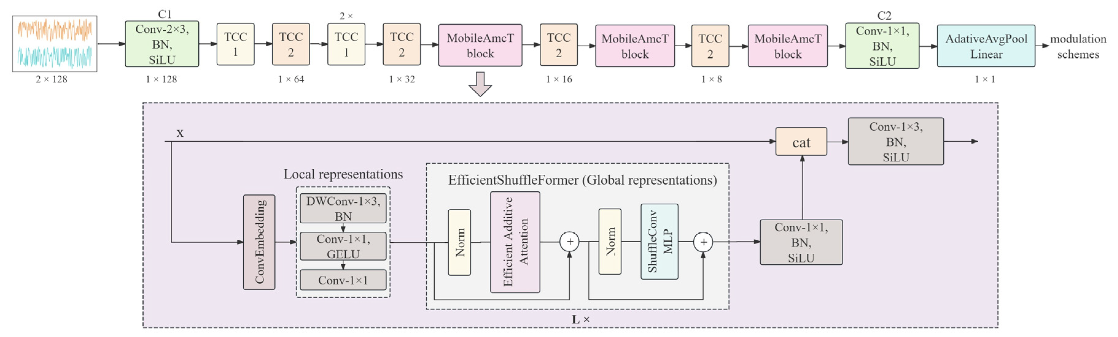
3.1. Model Framework

The MobileAmcT model integrates lightweight convolutional neural networks with efficient Transformer technology, aiming to provide an efficient and lightweight solution for automatic modulation classification tasks. This design optimizes the local processing capabilities of convolutional networks and the global information learning capabilities of Transformers, thereby achieving efficient feature extraction and fusion.

As shown in Figure 3, the model architecture includes an initial convolution layer C1, Token and Channel Conv (TCC) modules, MobileAmcT Blocks, an information fusion convolution layer C2, an adaptive global pooling layer, and a fully connected layer. Each part is dedicated to enhancing the efficiency of feature extraction and fusion. The data processing flow is as follows:

• Firstly, the model processes the input signal through the initial convolutional layer C1, which uses 2 × 3 convolutional kernels with a stride of 1, and integrates batch normalization (BN) and the SiLU activation function. This layer extracts low-level features from the signal and facilitates information exchange between I/Q channels.
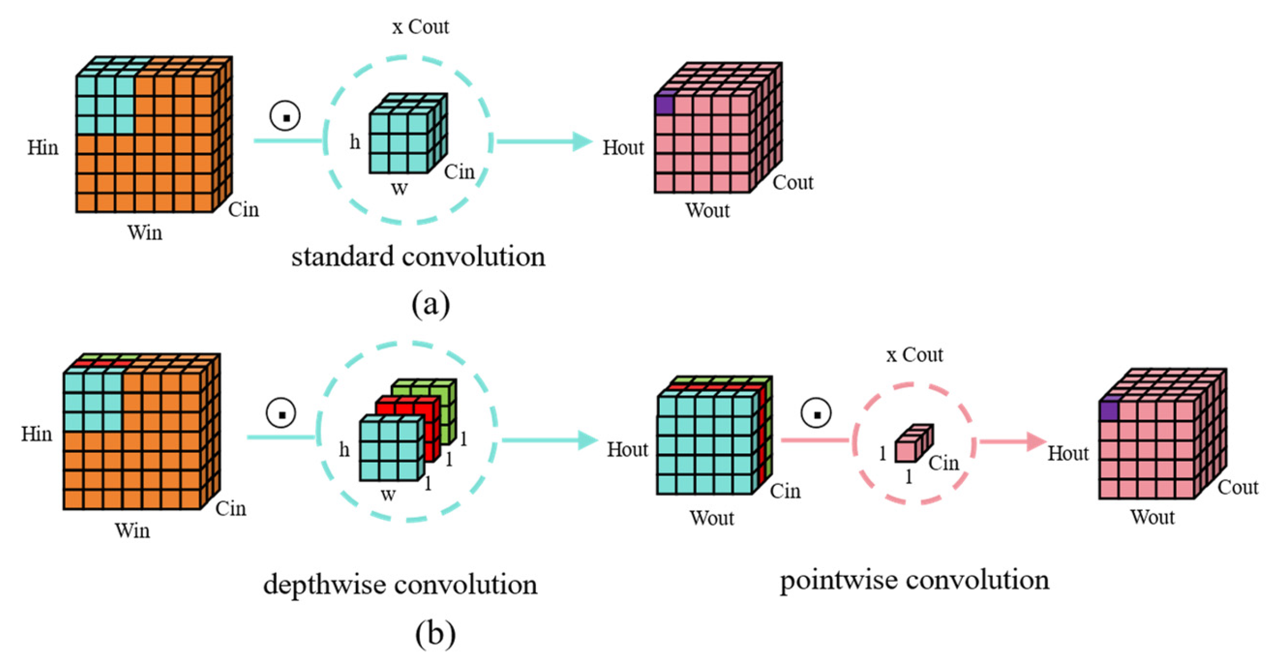
• Secondly, the intermediate TCC modules are divided into TCC1 and TCC2 modules. The TCC1 module combines depthwise convolution and channel attention mechanisms, focusing on efficient local feature extraction. This module efficiently extracts deep features through depthwise convolution and enhances feature representation using the channel attention mechanism. The TCC2 module further performs feature fusion and downsampling, extending the spatial range of features and enabling the model to effectively capture and process signal features at different scales.
• Thirdly, the core part of the model—the MobileAmcT Block—leverages lightweight convolution combined with the EfficientShuffleFormer to simultaneously handle local and global features. This module integrates the outputs of various layers through feature fusion techniques, forming a comprehensive feature representation, which significantly enhances the model’s performance in automatic modulation classification tasks.
• Finally, the information fusion convolutional layer C2 uses pointwise convolution to linearly combine the features from each channel, increasing the number of feature map channels and facilitating the capture of complex patterns. Finally, the adaptive global pooling layer and the fully connected layer work together to output the final classification results.

3.2. Key Module Design

3.2.1. TCC1 and TCC2 Modules

In recent studies, Yu et al. [36] proposed the innovative MetaFormer, a type of generalized architecture. As shown in Figure 4a, this architecture abstracts the structure of the Transformer network, isolating the Token Mixer and Channel Mixer modules. This highlights the importance of the general architecture behind the Transformer for model performance, providing a foundation for subsequent model designs. Building on the MetaFormer framework, this study combines MobileViT [37] and RepViT [38] technologies to propose lightweight convolutional neural network modules specifically designed for AMC tasks: the TCC1 module (with a stride of 1) and the TCC2 module (with a stride of 2).

• TCC1 Module

As shown in Figure 4b, the TCC1 module is designed for efficient local feature extraction and enhanced feature representation capabilities, comprising two parts: the Token Mixer and the Channel Mixer. The Token Mixer achieves feature fusion $X_f$ through a 1 × 1 depthwise convolution $W_{11}\in R^{C\times C}$, a 1 × 3 depthwise convolution $W_{13}\in R^{C\times C}$, and the original input $X\in R^{C\times H_0\times W_0}$, to capture features at different scales and effectively extract spatial information. The calculation process is shown in Equation (6), where $C$ represents the number of channels, $H_0$ is the feature height, and $W_0$ is the feature width. As shown in Figure 5, compared to traditional convolution, depthwise convolution operates independently on each channel, significantly reducing the number of parameters and computational complexity. The fused features are then processed by Batch Normalization (BN) and a squeeze-and-excitation (SE) module to obtain the token information, as described in Equation (7). Batch normalization is used to adjust the feature distribution, enhancing the model’s convergence speed and generalization ability. As illustrated in Figure 6, the SE module strengthens the model’s adaptive learning of channel importance by dynamically adjusting channel weights through fully connected layers and the Sigmoid activation function [39].

$$X_f=X{W}_{11}+X{W}_{13}+X$$

(6)

$$Y_t=SE(BN(X_f))$$

(7)

The Channel Mixer part includes a 1 × 1 expansion convolution $W_{11e}\in R^{C\times rC}$ and a 1 × 1 projection convolution $W_{11p}\in R^{rC\times C}$. These operations integrate all channel information through pointwise convolution and use the GELU activation function to optimize feature representation. Additionally, the Channel Mixer includes residual connections to facilitate effective gradient flow and deep model training, ultimately obtaining the mixed channel information, as described in Equation (8).

$$Y_c=BN(GELU(BN(Y_t{W}_{11e}))W_{11p})+Y_t$$

(8)

2.

TCC2 Module

As shown in Figure 4c, the TCC2 module builds upon the TCC1 module, adjusted to extract features over a broader spatial range and perform downsampling. The Token Mixer employs a 1 × 3 depthwise convolution with a stride of 2 to accelerate the reduction of feature map size. Subsequently, features are finely adjusted through the SE module and batch normalization.

In the design of both modules, we paid particular attention to computational efficiency and parameter optimization. Recent studies have shown that adjusting the expansion ratio of the Channel Mixer and applying structured pruning [40,41] can reduce the model’s parameter count and computational requirements while maintaining performance. Therefore, in this paper, the Channel Mixer expansion ratios for the TCC1 and TCC2 modules are both set to 2 to achieve higher computational efficiency and model lightweighting.

3.2.2. MobileAmcT Block

As shown in Figure 3, the design of the MobileAmcT Block integrates the dual advantages of local feature extraction and global feature capture, accurately processing input data in a modular manner. In the input stage, the tensor $X$ is split into two paths: one serving as the fusion baseline and the other being enhanced by the ConvEmbedding layer to accommodate the processing requirements of the subsequent network. Next, the local representation module achieves detailed local feature extraction through depthwise convolution, pointwise convolution, and the GELU activation function. Subsequently, the data is processed through the EfficientShuffleFormer module, which integrates Efficient Additive Attention and ShuffleConvMLP to comprehensively enhance the expression of global features. After dimensionality reduction through a 1 × 1 convolution layer and feature fusion through a 1 × 3 convolution layer, a richer and more comprehensive feature representation is ultimately generated. This efficient modular combination strategy allows MobileAmcT to retain local feature details while fully leveraging global information, significantly improving performance in automatic modulation classification tasks.

Local Representation Learning

Firstly, the input tensor $X_{tcc}\in R^{C_{tcc}\times H_{tcc}\times W_{tcc}}$ is converted into an embedded tensor $X_{emb}\in R^{D\times H_s\times W_s}$ through the embedding layer by performing a convolution operation $W_{emb}\in R^{C_{tcc}\times D}$ with a kernel size of 1 × 3, a stride of 1, and padding of (0, 1), as shown in Equation (9). Where $C_{tcc}$, $H_{tcc}$, and $W_{tcc}$ are the increased number of channels, reduced feature height, and reduced feature width after the series of TCC modules, respectively, and $D$ is the hidden dimension of the EfficientShuffleFormer module, $H_s=H_{tcc}/s$, $W_s=W_{tcc}/s$, and $\mathrm{s}$ represents the stride of the convolution kernel. The embedding layer adjusts the feature dimensions of the input, increasing the number of channels from $C_{tcc}$ to the hidden dimension $D$ required by EfficientShuffleFormer, thereby enhancing the model’s initial parsing capability of the signal. Additionally, the local representation layer further extracts fine-grained local features $X_{local}\in R^{D\times H_s\times W_s}$ through depthwise convolution $W_{13}$ and pointwise convolution $W_{11}$, enhancing the model’s ability to capture spatial information. The calculation process is shown in Equation (10). Specifically, depthwise convolution is performed independently on each channel, focusing on capturing local spatial features, while pointwise convolution is applied across all channels, promoting the integration of information between channels. This design not only enhances the local feature representation capability of the input signal but also provides a solid foundation for global feature extraction and fusion. The entire process uses the GELU activation function to increase the network’s non-linear expressive power, facilitating the learning of more complex patterns.

$$X_{emb}=BN(X{W}_{emb})$$

(9)

$$X_{local}=(GELU((BN(X_{emb}{W}_{13}))W_{11}))W_{11}$$

(10)

Global Representation Learning

In EfficientShuffleFormer, we introduced the EfficientAdditiveAttention and ShuffleConvMLP modules based on the MetaFormer architecture to enhance global feature extraction and representation. The EfficientAdditiveAttention module primarily captures global dependencies, improving the context awareness of features, thereby generating enhanced intermediate feature representation $Y$. Simultaneously, ShuffleConvMLP, as the feedforward neural network part, further processes the intermediate features $Y$ by utilizing channel shuffling and depthwise separable convolution to enhance feature integration, ultimately outputting the global feature representation $Z$.

$$Y=EfficientAdditiveAttention(BN(X_{local}))+X_{local}$$

(11)

$$Z=ShuffleConvMLP(BN(Y))+Y$$

(12)

To address the high computational complexity in the self-attention mechanism of Transformer models, an Efficient Additive Attention mechanism (EfficientAdditiveAttention) [42] was designed. The traditional matrix multiplication operation in self-attention mechanisms, which scales quadratically with image resolution, becomes a performance bottleneck. The additive attention mechanism in this study replaces the traditional matrix multiplication with a linear element-wise multiplication operation, significantly reducing computational complexity.

The self-attention mechanism enhances feature representation by capturing dependencies between different positions in the input sequence. The computational process is as follows:

Given an input embedding matrix $X_{local}\in R^{n\times d}(n=H_s\cdot W_s,d=D)$, where $n$ is the number of tokens and $d$ is the hidden dimension, it is mapped to the query matrix $Q$, key matrix $K$, and value matrix $V$ as follows:

$$Q=X_{local}{W}_q,K=X_{local}{W}_k,V=X_{local}{W}_v$$

(13)

where $W_q$, $W_k$, $W_v\in R^{d\times d}$ are learnable weight matrices. Then, the dot product of the query matrix and the key matrix is computed and divided by the scaling factor $\sqrt{d}$ to obtain the attention scores matrix:

$$a={\displaystyle \frac{Q{K}^T}{\sqrt{d}}}$$

(14)

Next, the attention scores matrix is subjected to the softmax operation to obtain the attention weights matrix:

$$A=soft\max (a)$$

(15)

Finally, the attention weights matrix is multiplied with the value matrix $V$ to obtain the final attention output $X_{att}\in R^{n\times d}$:

$$X_{att}=AV$$

(16)

Although the self-attention mechanism can effectively capture global contextual information, its computational complexity is $O(n^{2}d)$, which results in a very high computational cost for high-resolution images and long sequences.

As shown in Figure 7, the Efficient Additive self-attention mechanism only requires query-key interactions followed by a linear transformation, without the need for explicit key-value interactions. The computation process is as follows:

The input matrix $X_{local}$ is transformed into a query matrix $Q$ and a key matrix $K$ using two matrices $W_q$ and $W_k$:

$$Q=X_{local}{W}_q,K=X_{local}{W}_k$$

(17)

where $Q,K\in R^{n\times d}$, $W_{\mathrm{q}},W_k\in R^{d\times d}$. Then, the query matrix $Q$ is multiplied by the learnable parameter vector $w_a\in R^d$ to learn the attention weights of the query, generating the global attention query vector $A\in R^n$:

$$A={\displaystyle \frac{Q\cdot w_a}{\sqrt{d}}}$$

(18)

Then, based on the learned attention weights, the query matrix is pooled to obtain a single global query vector $q\in R^d$:

$$q={\displaystyle \sum _{i=1}^n{A}_i\cdot Q_i}$$

(19)

Next, the global query vector $q$ is interactively encoded with the key matrix $K$ to generate the final context vector $X_{att}\in R^{n\times d}$:

$$X_{att}=Q_{nor}+F(K\cdot q)$$

(20)

Here, $Q_{nor}$ represents the normalized query matrix, and $F$ denotes the linear transformation. The Efficient Additive Attention mechanism significantly reduces computational complexity by simplifying operations while maintaining or enhancing model performance. This makes it particularly suitable for handling high-resolution images and long sequence data.

As shown in Figure 8a, in the Transformer model, the feedforward neural network (FFN) is typically designed as a Multi-Layer Perceptron (MLP) consisting of two linear transformations separated by a non-linear activation function. The traditional FFN maps the input features from the original dimension to a higher dimension, increasing the model’s expressiveness through non-linear activation, and then maps it back to the original dimension. While this design enhances the model’s expressive power, it also significantly increases computational complexity and the number of parameters.

To address this challenge, we designed ShuffleConvMLP based on ShuffleNet V2 [43] as the feedforward neural network component of EfficientShuffleFormer. As illustrated in Figure 8b, ShuffleConvMLP employs channel shuffling and depthwise separable convolution techniques. Through per-channel and pointwise convolution operations, it enhances the understanding of input feature diversity and the processing of fine-grained information. The specific operations are as follows:

Introducing the channel shuffling technique, the enhanced intermediate feature $Y\in R^{D\times H_s\times W_s}$ undergoes channel shuffling to ensure thorough interaction between different channel groups, thereby enhancing the model’s representational capability. This process yields the channel-shuffled feature $Y_{cs}$. Next, the channel halving technique is applied. The channel-shuffled feature $Y_{cs}$ is split into two branches, each with $D/2$ channels. One branch, $Y_{cs1}\in R^{D/2\times H_s\times W_s}$, is kept as an identity and directly passed through, while the other branch, $Y_{cs2}\in R^{D/2\times H_s\times W_s}$, undergoes a series of convolution operations where the input and output channel numbers remain the same during the convolutions.

$$Y_{cs}=ChannelShuffle(Y)$$

(21)

The convolution operations are as follows:

Firstly, a 1 × 1 convolution $W_{11}\in R^{D/2\times D/2}$ is applied to map the number of channels to a higher dimension, enhancing the model’s representational capacity by increasing the feature dimension. This is followed by a depthwise separable convolution operation, which includes a 1 × 3 depthwise convolution $W_{13}\in R^{D/2\times D/2}$; this spatial convolution is applied channel-wise, using a 1 × 3 convolutional filter for each input channel separately. Compared to traditional convolution, depthwise convolution significantly reduces the computational load and effectively extracts local spatial features. Additionally, it includes a 1 × 1 pointwise convolution operation $W_{11}\in R^{D/2\times D/2}$; this step applies a 1 × 1 convolutional filter to each spatial position to integrate information across different channels, mapping the number of channels back to the original dimension. This process enhances the model’s non-linear representational capacity, efficiently fusing information from different channels and improving feature representation while maintaining computational efficiency.

$$Y_{cs2-conv1}=RELU(BN(Y_{cs2}{W}_{11})W_{13})$$

(22)

$$Y_{cs2-conv2}=BN(Y_{cs2-conv1}{W}_{13})$$

(23)

$$Y_{cs2-conv3}=RELU(BN(Y_{cs2-conv2}{W}_{11}))$$

(24)

After the convolution operations, the branch $Y_{cs2-conv3}$ is concatenated with the identity branch $Y_{cs1}$, restoring the original number of channels. This process further enhances the representational capacity of the fused information from different branches. Through the ShuffleConvMLP module, EfficientShuffleFormer can more effectively handle complex modulation recognition tasks, optimizing both the model’s performance and computational efficiency.

4. Experimental Results and Analysis

In this section, we conducted extensive experiments and analyses on different datasets. A comparison with a series of state-of-the-art methods was carried out to demonstrate the superior performance of the proposed method, and ablation experiments were conducted to observe the robustness of MobileAmcT.

4.1. Experimental Settings

4.1.1. Experimental Platform and Hyperparameter Settings

In this study, the training and testing processes were performed in a Python 3.8.18 environment using PyTorch 1.10.2+cu113, running on an x86_64 architecture server equipped with an NVIDIA A100 GPU and an Intel(R) Xeon(R) Gold 5218R CPU @ 2.10 GHz. All models were trained end-to-end using the Adam optimizer, with the classification loss function set to cross-entropy loss. The initial learning rate was set to 4 × 10⁻³ with a learning rate adjustment rate of 0.8. The models were trained for 100 epochs with each batch containing 400 input samples. For each dataset, the ratio of the training set, validation set, and test set was allocated as 6:2:2.

4.1.2. Experimental Dataset

To evaluate and validate the effectiveness of the proposed AMC method, we utilized the RadioML2016.10a dataset generated by GNU Radio for the modulation classification task. The parameters of the public dataset RadioML2016.10a are listed in

Table 1. Parameters of RadioML2016.10a dataset.

Parameters	Contents
Modulation types	8PSK, BPSK, CPFSK, GFSK, PAM4, 16QAM, AM-DSB, AM-SSB, 64QAM, QPSK, WBFM
Sample length	2 × 128
SNR (dB)	−20:2:18
Number	220,000
Standard deviation of the sampling rate offset	0.01 Hz
Maximum sample rate offset	50 Hz
Carrier frequency offset standard deviation	0.01 Hz
Maximum carrier frequency offset	500 Hz
No. of sine waves in frequency selective fading	8
Sampling rate	200 kHz

. This dataset comprises two data sources: analog modulation using real continuous speech signals from the publicly accessible Serial Episode No. 1, and digital modulation using the Gutenberg edition of Shakespeare’s works, which were whitened using a block normalizer to ensure uniform data distribution. To simulate the effects of unknown scaling and translation, the synthetic signals were transmitted through multiple channels. The dataset was then generated by the GNU Radio channel model unit, which simulates real communication transmission environments by adding various interference factors such as AWGN, selective fading (including Rician and Rayleigh fading), center frequency offset, and multipath fading [35]. This unit used a rectangular window of length 128 to segment the time-series signals, with each sample containing raw data of two in-phase and quadrature (I/Q) channels, sized 2 × 128. The dataset contains 220,000 modulation signals, including eleven types of modulation: eight digital modulations and three analog modulations, which are frequently used in wireless communication networks. The digital modulations include BPSK, 8PSK, CPFSK, GFSK, 16QAM, 64QAM, and PAM4, while the analog modulations include AM-DSB, WB-FM, and AM-SSB. The signal-to-noise ratio (SNR) ranges from −20 dB to 18 dB, with an incremental step of 2 dB.

4.2. Comparison with Model Parameter Setting

In the MobileAmcT model, the spatial dimensions of the feature maps are $T_i(i=0,\dots ,10)$, and the number of layers in the EfficientShuffleFormer of the three MobileAmcT Blocks is $L$, with a hidden dimension of $D$. To comprehensively evaluate the impact of different parameter configurations on the performance of the MobileAmcT model, we designed three different network scales: MobileAmcT-S, MobileAmcT-M, and MobileAmcT-L, with the parameter settings shown in

Table 2. The computational cost and accuracy of the architecture with various parameter settings on RadioML2016.10a.

		MobileAmcT-S	MobileAmcT-M	MobileAmcT-L
Parameter Settings	L	2, 4, 3	2, 4, 3	2, 4, 3
	D	48, 64, 80	64, 80, 96	96, 120, 144
	$T_i(i=0,\dots ,10)$	8, 8, 16, 16, 24, 24, 32, 32, 48, 48, 256	16, 16, 24, 24, 48, 48, 64, 64, 80, 80, 320	32, 32, 48, 48, 64, 64, 80, 80, 96, 96, 384
Parameters		310,752	575,064	1,146,440
FLOPs		4,717,248	8,899,328	18,516,160
Average Accuracy		62.58%	62.93%	62.38%

. These three configurations aim to explore the relationship between the number of model parameters and classification accuracy, identifying the optimal model structure in terms of balancing resource usage and performance.

The parameters, floating-point operations (FLOPs), and average accuracy levels shown in Table 2 are key metrics for comparing different models. Parameters represent the total number of learnable weights in the model, while FLOPs measure the computational cost of the model. Average accuracy is the mean classification accuracy of the model across all SNR conditions in the test set, calculated as the ratio of the number of correctly predicted samples to the total number of samples under all SNR conditions. It provides a unified metric for quickly comparing the overall performance of different models, reflecting the model’s general capability and robustness in various environments, and serves as a crucial indicator for evaluating model effectiveness. These metrics are also used in the remaining tables.

As shown in Figure 9, the accuracy parameters shown in the figure represent the classification accuracy of the model at each SNR value on the test set, which is the ratio of the number of correctly predicted samples to the total number of samples at that SNR value, demonstrating the model’s performance under different SNR conditions. The accuracy parameters in the remaining figures have the same meaning as those in Figure 9. The experimental results indicate that the medium-sized MobileAmcT-M demonstrates the highest average classification accuracy across various signal-to-noise ratio (SNR) settings, outperforming the more parameter-heavy MobileAmcT-S and the more parameter-efficient MobileAmcT-L. Specifically, despite MobileAmcT-S having higher theoretical computational capabilities, its actual performance is hindered, possibly due to overfitting and increased model complexity. On the other hand, MobileAmcT-L, while suitable for resource-constrained environments, lacks sufficient capability to capture complex signal features, leading to a decline in performance. This finding suggests that merely increasing the model size is not always the optimal strategy in designing deep learning models. In particular, for automatic modulation classification tasks, a moderate model size (as exemplified by MobileAmcT-M) can more effectively balance performance and computational resource usage, thereby achieving broad applicability and efficient performance in different operating environments.

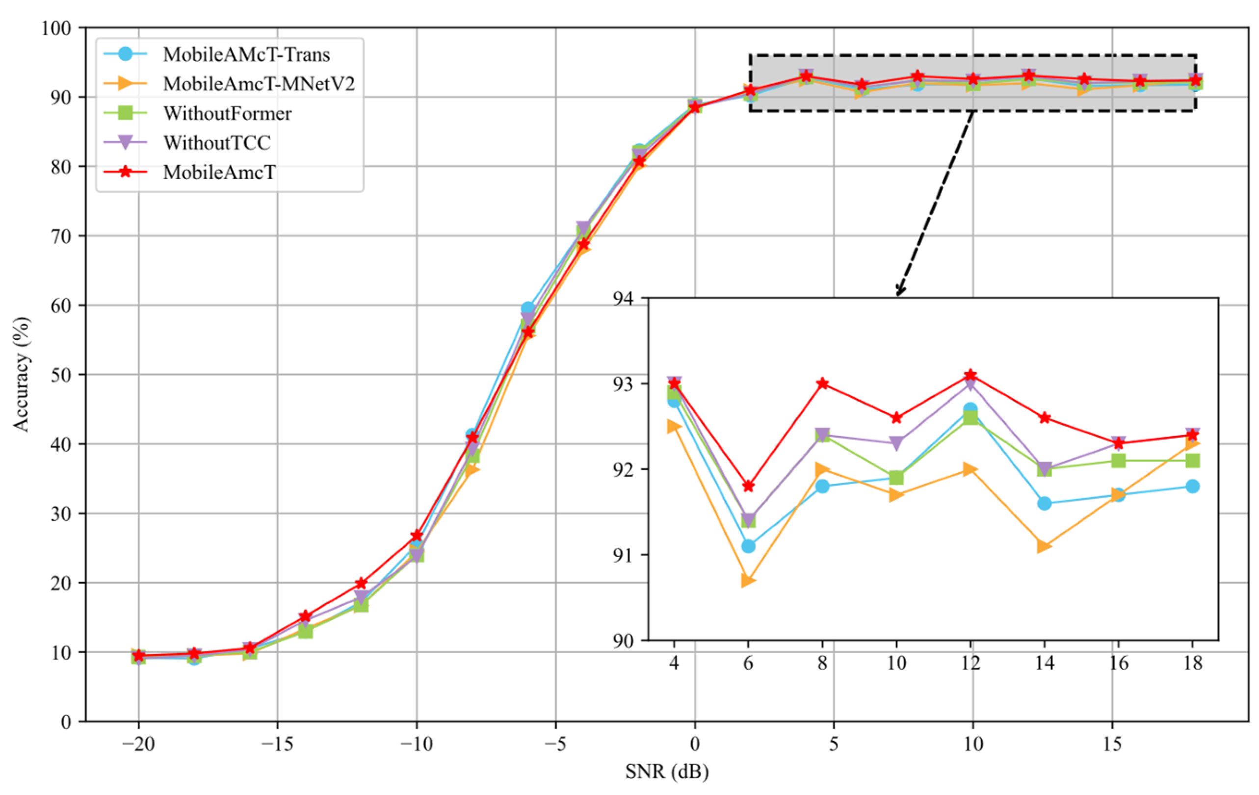
4.3. Evaluating Modules in MobileAmcT Model

Through the following experiments, we systematically evaluated the impact of various modules in the MobileAmcT model on the performance of AMC tasks to further optimize the model structure. The classification accuracy, parameters, and floating-point operations (FLOPs) for each ablation experiment are shown in

Table 3. Performance comparison of different ablated models in MobileAmcT on RadioML2016.10a.

Model Variation	Average Accuracy	Parameters	FLOPs
MobileAmcT-Trans	62.65%	1,135,016	8,454,032
MobileAmcT-MNetV2	61.84%	540,352	8,578,176
WithoutFormer	62.35%	290,856	4,748,672
WithoutTCC	62.64%	521,120	66,596,608
MobileAmcT	62.93%	575,064	8,899,328

, and the experimental results are illustrated in Figure 10.

4.3.1. Importance Analysis of Global Feature Extraction Module (MobileAmcT-Trans)

In this ablation experiment, we replaced the EfficientShuffleFormer module in the MobileAmcT model with a traditional Transformer module, forming the MobileAmcT-Trans model. Although MobileAmcT-Trans increased the parameter count by approximately 97.3% (from 575,064 to 1,135,016) and reduced FLOPs by 5%, its average classification accuracy dropped from 62.93% to 62.65%. This indicates the critical role of EfficientShuffleFormer in efficient global feature extraction. Despite the strong modeling capabilities of the traditional Transformer, the significant increase in parameter count may lead to overfitting, thereby affecting overall performance. Specifically, at an SNR of 12 dB, the classification accuracy of MobileAmcT-Trans was 92.7%, slightly lower than MobileAmcT’s 93.1%, further confirming the advantages of EfficientShuffleFormer.

4.3.2. Suitability Analysis of Local Feature Extraction Module (MobileAmcT-MNetV2)

By replacing the TCC module with MobileNet-V2’s Inverted Residual Block, experimental results show that the parameter count of MobileAmcT-MNetV2 was reduced by 6%, while FLOPs slightly increased by 3.6%. However, the classification accuracy dropped by 1.09%. Under certain SNR conditions, such as 6 dB, the accuracy of MobileAmcT-MNetV2 was 90.7%, lower than MobileAmcT’s 91.8%. This result highlights the advantage of the TCC module in capturing subtle variations in modulation signals. The TCC module is specially designed to more effectively handle the time series characteristics of automatic modulation classification tasks, while the structure of MobileNet-V2 performs worse in this specific task.

4.3.3. Impact Verification of Global Feature Extraction Module (WithoutFormer)

To verify the role of the EfficientShuffleFormer module, we completely removed this module. The experimental results show that the parameter count and FLOPs of the WithoutFormer model were reduced by 49.4% and 46.6%, respectively, but the classification accuracy also dropped by 0.58%. For example, at 10 dB, the accuracy of WithoutFormer was 91.9%, while MobileAmcT’s accuracy was 92.6%. This indicates the significant role of the EfficientShuffleFormer module in enhancing global feature representation and fusion capabilities. The combination of EfficientAdditiveAttention and ShuffleConvMLP significantly enhances the model’s ability to capture features, especially under higher SNR conditions, where the performance is particularly outstanding.

4.3.4. Performance Impact of Local Feature Extraction Module (WithoutTCC)

We removed the TCC module from the MobileAmcT model, forming the WithoutTCC model. The experimental data shows that the parameter count of WithoutTCC was reduced by 9.4%, and the classification accuracy dropped by 0.31%. Under low SNR conditions, such as −6 dB, the accuracy of WithoutTCC was only 57.9%, while MobileAmcT’s accuracy was 56.1%. Although the performances were similar under some high SNR conditions (e.g., 18 dB), overall, the core role of the TCC module in local feature extraction and performance improvement is evident. A well-designed local processing module is crucial for maintaining high classification accuracy, especially when dealing with complex signals, where the advantages of the TCC module are more pronounced.

In summary, the experimental results indicate that MobileAmcT performs significantly better than other variant models under various SNR conditions, validating the importance of the EfficientShuffleFormer and TCC modules in improving model performance and reducing computational complexity. These results further emphasize the effectiveness of innovative module design in feature extraction and fusion.

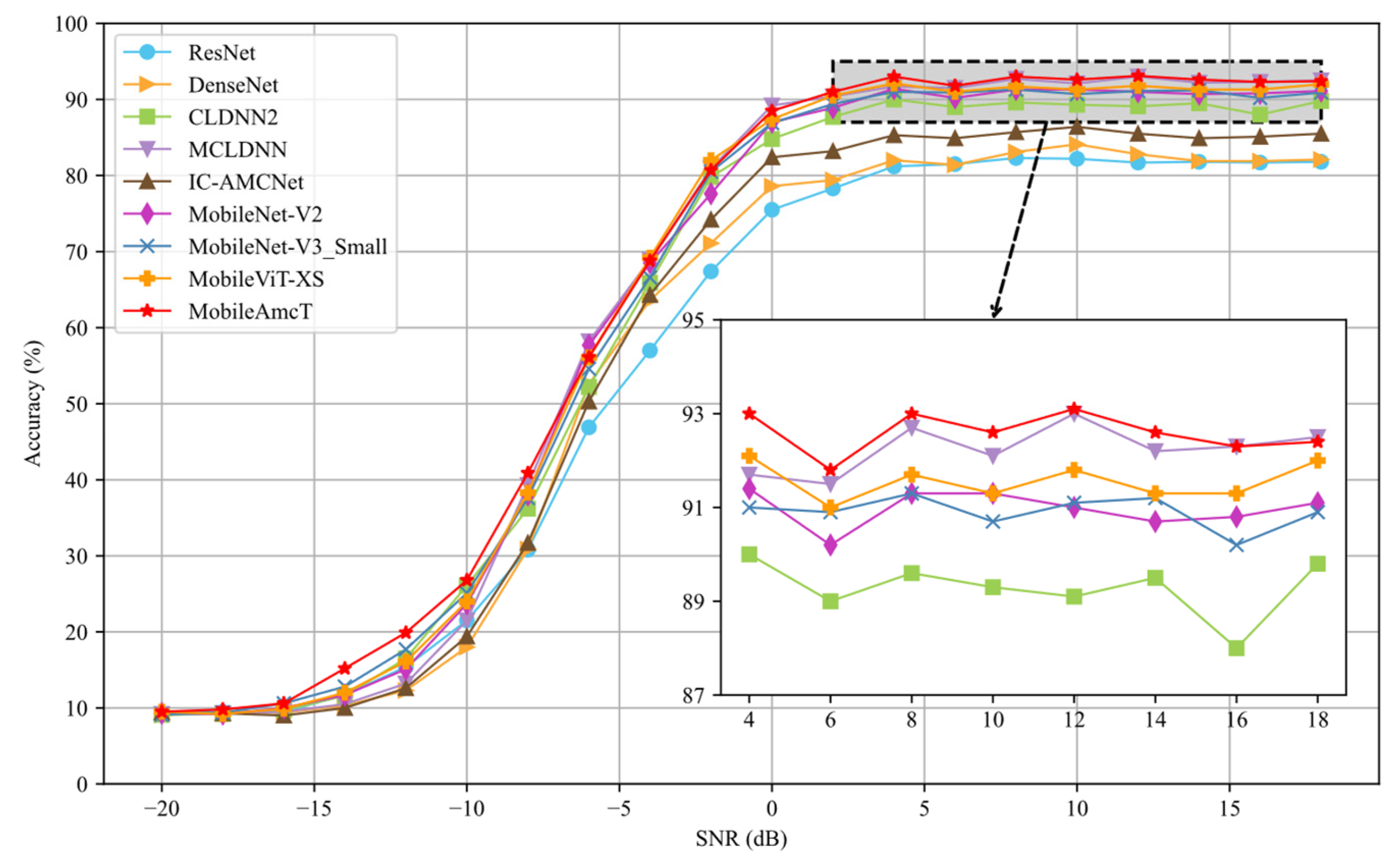
4.4. Performance Comparison between Different Methods

In this study, we propose a lightweight model specifically designed for automatic modulation classification tasks, named MobileAmcT. We compared MobileAmcT with several representative AMC models, including ResNet [44], DenseNet [44], CLDNN2 [45], MCLDNN [46], and IC-AMCNet [47]. Additionally, we compared it with several state-of-the-art lightweight models commonly used for vision tasks, including MobileNet-V2 [48], MobileNet-V3_Small [49], and MobileViT-XS [32].

Figure 11 illustrates the variation in classification accuracy with increasing signal-to-noise ratios (SNR) for different methods on the RadioML2016.10a dataset. Notably, our proposed MobileAmcT model achieves an average accuracy of only 9.5% at an SNR of −20 dB. However, as the SNR increases to 0 dB, the accuracy significantly improves to 88.5%. Furthermore, at an SNR of 12 dB, the classification accuracy reaches its highest value of 93.1%. This improvement in accuracy is primarily attributed to the enhanced signal quality and reduced noise interference with increasing SNR, enabling the model to more effectively extract and recognize signal features, thereby significantly enhancing classification performance.

Our experimental results demonstrate that MobileAmcT performs excellently across all SNR environments, with its classification accuracy significantly surpassing other representative AMC models. Moreover, compared to advanced lightweight models, MobileAmcT not only maintains high accuracy but also significantly reduces the number of parameters and computational complexity, proving its potential in practical applications. Specifically, under an SNR of 12 dB, MobileAmcT achieves the highest classification accuracy of 93.1%, exceeding the other compared methods by up to 11.4%.

Additionally,

Table 4. Performance comparison of different methods on RadioML2016.10a.

Dataset	Model	Average Accuracy	Parameters	FLOPs
RadioML2016.10a	ResNet [43]	54.35%	3,098,283	248,425,410
	DenseNet [43]	55.20%	3,282,603	342,797,250
	CLDNN2 [44]	60.16%	517,643	117,635,426
	MCLDNN [45]	61.91%	406,070	35,773,612
	IC-AMCNet [46]	56.96%	1,264,011	29,686,722
	MobileNet-V2 [47]	61.23%	2,194,475	24,250,880
	MobileNet-V3_Small [48]	61.38%	1,636,483	19,411,840
	MobileViT-XS [32]	61.84%	1,639,952	27,083,296
	MobileAmcT (proposed)	62.93%	575,064	8,899,328

presents the classification accuracy, parameter count, and FLOPs (floating-point operations) for various models on the RML2016.10a dataset. On this dataset, MobileAmcT achieves an average accuracy of 0.6293 with 575,064 parameters and 8,899,328 FLOPs, outperforming other models. Specifically, ResNet has 3,098,283 parameters and 248,425,410 FLOPs, but its average accuracy is only 0.5435. Compared to ResNet, MobileAmcT reduces the parameter count by 81.4% and FLOPs by 96.4%, while increasing accuracy by 8.58%. DenseNet has 3,282,603 parameters, 342,797,250 FLOPs, and an average accuracy of 0.5520. In contrast, MobileAmcT reduces the parameter count by 82.5% and FLOPs by 97.4%, with a 7.74% increase in accuracy. MobileAmcT achieves higher classification accuracy with fewer parameters and lower computational complexity compared to more complex models like ResNet, DenseNet, and IC-AMCNet. For other AMC models, although CLDNN2 and MCLDNN have fewer parameters, their accuracy is still lower than that of MobileAmcT. Regarding advanced lightweight network models such as MobileNet-V2, MobileNet-V3_Small, and MobileViT-XS, MobileAmcT surpasses them in terms of parameter count, FLOPs, and average accuracy. Overall, MobileAmcT demonstrates higher efficiency and superior performance.

To further analyze the classification performance of the MobileAmcT model, confusion matrices were presented for different SNR conditions (−10 dB, 0 dB, 10 dB, 18 dB) on the RadioML2016.10a dataset. As shown in Figure 12, at an SNR of −10 dB, the significant noise causes difficulty in distinguishing modulation types, often misclassifying multiple signals as AM-SSB modulation, with an accuracy of only 26.8%. When the SNR improves to 0 dB, the classification accuracy significantly increases to 88.5%, although there is still noticeable confusion between WBFM and AM-DSB, mainly due to both being continuous analog voice signals. Confusion between QPSK and 8PSK is also common since the constellation points of 8PSK are a subdivision of QPSK. As the SNR further increases to 6 dB and 12 dB, the classification performance continues to improve, reaching a high of 93.1% at 12 dB, with all modulation types accurately recognized except for some remaining confusion between WBFM and AM-DSB.

5. Conclusions

AMC ensures reliable and efficient communication for drone systems in various non-cooperative environments, playing a critical role in drone communications. In this study, we propose the MobileAmcT model, which introduces innovative TCC1 and TCC2 modules and the EfficientShuffleFormer module, providing an efficient and lightweight solution for automatic modulation classification (AMC) tasks. The TCC modules focus on efficiently capturing local features of the signals, while the EfficientShuffleFormer module combines Efficient Additive Attention and ShuffleConvMLP technologies to optimize the fusion and expression of global features. Experimental results on the RadioML2016.10a dataset demonstrate that MobileAmcT maintains low computational complexity and parameter count under various signal-to-noise ratio (SNR) conditions while achieving outstanding classification accuracy, significantly surpassing existing models. Specifically, compared to ResNet, DenseNet, and IC-AMCNet, which have more parameters and more complex structures, MobileAmcT reduces parameter counts by 81.4%, 82.5%, and 54.5%, respectively, while improving accuracy by 8.58%, 7.74%, and 5.98%. These results highlight the potential and practical value of MobileAmcT for deployment in resource-constrained drone communication devices.

References

1. Liu, M.; Liao, G.; Zhao, N.; Song, H.; Gong, F. Data-driven deep learning for signal classification in industrial cognitive radio networks. IEEE Trans. Ind. Inform. 2020, 17, 3412–3421. [Google Scholar] [CrossRef]
2. Ma, J.; Liu, H.; Peng, C.; Qiu, T. Unauthorized broadcasting identification: A deep LSTM recurrent learning approach. IEEE Trans. Instrum. Meas. 2020, 69, 5981–5983. [Google Scholar] [CrossRef]
3. Chang, S.; Huang, S.; Zhang, R.; Feng, Z.; Liu, L. Multitask-learning-based deep neural network for automatic modulation classification. IEEE Internet Things J. 2021, 9, 2192–2206. [Google Scholar] [CrossRef]
4. Dobre, O.A.; Abdi, A.; Bar-Ness, Y.; Su, W. Survey of automatic modulation classification techniques: Classical approaches and new trends. IET Commun. 2007, 1, 137–156. [Google Scholar] [CrossRef]
5. Tadaion, A.; Derakhtian, M.; Gazor, S.; Aref, M. Likelihood ratio tests for PSK modulation classification in unknown noise environment. In Proceedings of the Canadian Conference on Electrical and Computer Engineering, Saskatoon, SK, Canada, 1–4 May 2005; pp. 151–154. [Google Scholar]
6. Xu, J.L.; Su, W.; Zhou, M. Likelihood-ratio approaches to automatic modulation classification. IEEE Trans. Syst. Man Cybern. Part C (Appl. Rev.) 2010, 41, 455–469. [Google Scholar] [CrossRef]
7. Xie, L.; Wan, Q. Cyclic feature-based modulation recognition using compressive sensing. IEEE Wirel. Commun. Lett. 2017, 6, 402–405. [Google Scholar] [CrossRef]
8. Li, T.; Li, Y.; Dobre, O.A. Modulation classification based on fourth-order cumulants of superposed signal in NOMA systems. IEEE Trans. Inf. Forensics Secur. 2021, 16, 2885–2897. [Google Scholar] [CrossRef]
9. Gardner, W.A.; Spooner, C.M. Cyclic spectral analysis for signal detection and modulation recognition. In Proceedings of the MILCOM 88, 21st Century Military Communications-What’s Possible? Conference Record. Military Communications Conference, San Diego, CA, USA, 23–26 October 1988; pp. 419–424. [Google Scholar]
10. Hazza, A.; Shoaib, M.; Alshebeili, S.A.; Fahad, A. An overview of feature-based methods for digital modulation classification. In Proceedings of the 2013 1st International Conference on Communications, Signal Processing, and Their Applications (ICCSPA), Sharjah, United Arab Emirates, 12–14 February 2013; pp. 1–6. [Google Scholar]
11. Zheng, S.; Zhou, X.; Zhang, L.; Qi, P.; Qiu, K.; Zhu, J.; Yang, X. Towards next-generation signal intelligence: A hybrid knowledge and data-driven deep learning framework for radio signal classification. IEEE Trans. Cogn. Commun. Netw. 2023, 9, 564–579. [Google Scholar] [CrossRef]
12. Wang, Y.; Liu, M.; Yang, J.; Gui, G. Data-driven deep learning for automatic modulation recognition in cognitive radios. IEEE Trans. Veh. Technol. 2019, 68, 4074–4077. [Google Scholar] [CrossRef]
13. Huang, S.; Lin, C.; Xu, W.; Gao, Y.; Feng, Z.; Zhu, F. Identification of active attacks in Internet of Things: Joint model-and data-driven automatic modulation classification approach. IEEE Internet Things J. 2020, 8, 2051–2065. [Google Scholar] [CrossRef]
14. Zheng, Q.; Zhao, P.; Li, Y.; Wang, H.; Yang, Y. Spectrum interference-based two-level data augmentation method in deep learning for automatic modulation classification. Neural Comput. Appl. 2021, 33, 7723–7745. [Google Scholar] [CrossRef]
15. Wang, Y.; Gui, G.; Ohtsuki, T.; Adachi, F. Multi-task learning for generalized automatic modulation classification under non-Gaussian noise with varying SNR conditions. IEEE Trans. Wirel. Commun. 2021, 20, 3587–3596. [Google Scholar] [CrossRef]
16. Ma, K.; Zhou, Y.; Chen, J. CNN-based automatic modulation recognition of wireless signal. In Proceedings of the 2020 IEEE 3rd International Conference on Information Systems and Computer Aided Education (ICISCAE), Dalian, China, 27–29 September 2020; pp. 654–659. [Google Scholar]
17. Zeng, Y.; Zhang, M.; Han, F.; Gong, Y.; Zhang, J. Spectrum analysis and convolutional neural network for automatic modulation recognition. IEEE Wirel. Commun. Lett. 2019, 8, 929–932. [Google Scholar] [CrossRef]
18. Daldal, N.; Yıldırım, Ö.; Polat, K. Deep long short-term memory networks-based automatic recognition of six different digital modulation types under varying noise conditions. Neural Comput. Appl. 2019, 31, 1967–1981. [Google Scholar] [CrossRef]
19. Zheng, Q.; Tian, X.; Yu, Z.; Wang, H.; Elhanashi, A.; Saponara, S. DL-PR: Generalized automatic modulation classification method based on deep learning with priori regularization. Eng. Appl. Artif. Intell. 2023, 122, 106082. [Google Scholar] [CrossRef]
20. Hong, D.; Zhang, Z.; Xu, X. Automatic modulation classification using recurrent neural networks. In Proceedings of the 2017 3rd IEEE International Conference on Computer and Communications (ICCC), Chengdu, China, 13–16 December 2017; pp. 695–700. [Google Scholar]
21. Sümen, G.; Çelebi, B.A.; Kurt, G.K.; Görçin, A.; Başaran, S.T. Multi-Channel Learning with Preprocessing for Automatic Modulation Order Separation. In Proceedings of the 2022 IEEE Symposium on Computers and Communications (ISCC), Rhodes, Greece, 30 June–3 July 2022; pp. 1–5. [Google Scholar]
22. Zhang, Z.; Luo, H.; Wang, C.; Gan, C.; Xiang, Y. Automatic modulation classification using CNN-LSTM based dual-stream structure. IEEE Trans. Veh. Technol. 2020, 69, 13521–13531. [Google Scholar] [CrossRef]
23. Liu, Y.; Liu, Y.; Yang, C. Modulation recognition with graph convolutional network. IEEE Wirel. Commun. Lett. 2020, 9, 624–627. [Google Scholar] [CrossRef]
24. Tonchev, K.; Neshov, N.; Ivanov, A.; Manolova, A.; Poulkov, V. Automatic modulation classification using graph convolutional neural networks for time-frequency representation. In Proceedings of the 2022 25th International Symposium on Wireless Personal Multimedia Communications (WPMC), Herning, Denmark, 30 October–2 November 2022; pp. 75–79. [Google Scholar]
25. Zheng, Q.; Zhao, P.; Wang, H.; Elhanashi, A.; Saponara, S. Fine-grained modulation classification using multi-scale radio transformer with dual-channel representation. IEEE Commun. Lett. 2022, 26, 1298–1302. [Google Scholar] [CrossRef]
26. Kong, W.; Yang, Q.; Jiao, X.; Niu, Y.; Ji, G. A transformer-based CTDNN structure for automatic modulation recognition. In Proceedings of the 2021 7th International Conference on Computer and Communications (ICCC), Chengdu, China, 10–13 December 2021; pp. 159–163. [Google Scholar]
27. Chen, Y.; Dong, B.; Liu, C.; Xiong, W.; Li, S. Abandon locality: Frame-wise embedding aided transformer for automatic modulation recognition. IEEE Commun. Lett. 2022, 27, 327–331. [Google Scholar] [CrossRef]
28. Iandola, F.N.; Han, S.; Moskewicz, M.W.; Ashraf, K.; Dally, W.J.; Keutzer, K. SqueezeNet: AlexNet-level accuracy with 50x fewer parameters and< 0.5 MB model size. arXiv preprint 2016, arXiv:1602.07360. [Google Scholar]
29. Howard, A.G.; Zhu, M.; Chen, B.; Kalenichenko, D.; Wang, W.; Weyand, T.; Andreetto, M.; Adam, H. Mobilenets: Efficient convolutional neural networks for mobile vision applications. arXiv 2017, arXiv:1704.04861. [Google Scholar]
30. Zhang, X.; Zhou, X.; Lin, M.; Sun, J. Shufflenet: An extremely efficient convolutional neural network for mobile devices. In Proceedings of the IEEE Conference on Computer Vision and Pattern Recognition, Salt Lake City, UT, USA, 18–22 June 2018; pp. 6848–6856. [Google Scholar]
31. Chen, Y.; Dai, X.; Chen, D.; Liu, M.; Dong, X.; Yuan, L.; Liu, Z. Mobile-former: Bridging mobilenet and transformer. In Proceedings of the IEEE/CVF Conference on Computer Vision and Pattern Recognition, New Orleans, LA, USA, 18–24 June 2022; pp. 5270–5279. [Google Scholar]
32. Mehta, S.; Rastegari, M. Mobilevit: Light-weight, general-purpose, and mobile-friendly vision transformer. arXiv 2021, arXiv:2110.02178. [Google Scholar]
33. Vaswani, A.; Shazeer, N.; Parmar, N.; Uszkoreit, J.; Jones, L.; Gomez, A.N.; Kaiser, Ł.; Polosukhin, I. Attention is all you need. In Proceedings of the 31st Conference on Neural Information Processing Systems (NIPS 2017), Long Beach, CA, USA, 4–9 December 2017. [Google Scholar]
34. Dosovitskiy, A.; Beyer, L.; Kolesnikov, A.; Weissenborn, D.; Zhai, X.; Unterthiner, T.; Dehghani, M.; Minderer, M.; Heigold, G.; Gelly, S. An image is worth 16 × 16 words: Transformers for image recognition at scale. arXiv 2020, arXiv:2010.11929. [Google Scholar]
35. O’shea, T.J.; West, N. Radio machine learning dataset generation with gnu radio. In Proceedings of the GNU Radio Conference, Boulder, CO, USA, 12–16 September 2016; Volume 1. [Google Scholar]
36. Yu, W.; Luo, M.; Zhou, P.; Si, C.; Zhou, Y.; Wang, X.; Feng, J.; Yan, S. Metaformer is actually what you need for vision. In Proceedings of the IEEE/CVF Conference on Computer Vision and Pattern Recognition, New Orleans, LA, USA, 18–24 June 2022; pp. 10819–10829. [Google Scholar]
37. Mehta, S.; Rastegari, M. Separable self-attention for mobile vision transformers. arXiv preprint 2022, arXiv:2206.02680. [Google Scholar]
38. Wang, A.; Chen, H.; Lin, Z.; Han, J.; Ding, G. Repvit: Revisiting mobile cnn from vit perspective. arXiv 2023, arXiv:2307.09283. [Google Scholar]
39. Hu, J.; Shen, L.; Sun, G. Squeeze-and-excitation networks. In Proceedings of the IEEE Conference on Computer Vision and Pattern Recognition, Salt Lake City, UT, USA, 18–22 June 2018; pp. 7132–7141. [Google Scholar]
40. Graham, B.; El-Nouby, A.; Touvron, H.; Stock, P.; Joulin, A.; Jégou, H.; Douze, M. Levit: A vision transformer in convnet’s clothing for faster inference. In Proceedings of the IEEE/CVF International Conference on Computer Vision, Montreal, BC, Canada, 11–17 October 2021; pp. 12259–12269. [Google Scholar]
41. Yang, H.; Yin, H.; Molchanov, P.; Li, H.; Kautz, J. Nvit: Vision Transformer Compression and Parameter Redistribution. Available online: https://openreview.net/forum?id=LzBBxCg-xpa (accessed on 21 March 2023).
42. Shaker, A.; Maaz, M.; Rasheed, H.; Khan, S.; Yang, M.-H.; Khan, F.S. Swiftformer: Efficient additive attention for transformer-based real-time mobile vision applications. In Proceedings of the IEEE/CVF International Conference on Computer Vision, Paris, France, 2–6 October 2023; pp. 17425–17436. [Google Scholar]
43. Ma, N.; Zhang, X.; Zheng, H.T.; Sun, J. Shufflenet v2: Practical guidelines for efficient cnn architecture design. In Proceedings of the European Conference on Computer Vision (ECCV), Munich, Germany, 8–14 September 2018; pp. 116–131. [Google Scholar]
44. Liu, X.; Yang, D.; El Gamal, A. Deep neural network architectures for modulation classification. In Proceedings of the 2017 51st Asilomar Conference on Signals, Systems, and Computers, Pacific Grove, CA, USA, 29 October–1 November 2017; pp. 915–919. [Google Scholar]
45. West, N.E.; O’shea, T. Deep architectures for modulation recognition. In Proceedings of the 2017 IEEE International Symposium on Dynamic Spectrum Access Networks (DySPAN), Baltimore, MD, USA, 6–9 March 2017; pp. 1–6. [Google Scholar]
46. Xu, J.; Luo, C.; Parr, G.; Luo, Y. A spatiotemporal multi-channel learning framework for automatic modulation recognition. IEEE Wirel. Commun. Lett. 2020, 9, 1629–1632. [Google Scholar] [CrossRef]
47. Hermawan, A.P.; Ginanjar, R.R.; Kim, D.S.; Lee, J.-M. CNN-based automatic modulation classification for beyond 5G communications. IEEE Commun. Lett. 2020, 24, 1038–1041. [Google Scholar] [CrossRef]
48. Sandler, M.; Howard, A.; Zhu, M.; Zhmoginov, A.; Chen, L.-C. Mobilenetv2: Inverted residuals and linear bottlenecks. In Proceedings of the IEEE Conference on Computer Vision and Pattern Recognition, Salt Lake City, UT, USA, 18–22 June 2018; pp. 4510–4520. [Google Scholar]
49. Howard, A.; Sandler, M.; Chu, G.; Chen, L.-C.; Chen, B.; Tan, M.; Wang, W.; Zhu, Y.; Pang, R.; Vasudevan, V. Searching for MobileNetV3. In Proceedings of the IEEE/CVF International Conference on Computer Vision, Seoul, Republic of Korea, 27 October–2 November 2019; pp. 1314–1324. [Google Scholar]
Figure 1. System architecture for automatic modulation classification.
Drones 08 00357 g001
Figure 2. Modulation type I/Q signal waveforms from the RadioML2016.10a dataset: (a) QAM64, (b) QPSK, (c) AM-DSB, (d) 8PSK.
Drones 08 00357 g002
Figure 3. Specific structure of MobileAmcT.
Drones 08 00357 g003
Figure 4. (a) MetaFormer general architecture, (b) TCC1 Block with stride of 1, (c) TCC2 Block with stride of 2. Here, DWConv-1xn represents a 1 × n depthwise convolution, Conv-1x1-e represents a standard 1 × 1 convolution used for expansion, and Conv-1x1-p refers to a standard 1 × 1 convolution used for projection. Blocks that perform downsampling are marked with ↓2.
Drones 08 00357 g004
Figure 5. Comparison of depthwise convolution, pointwise convolution, and standard convolution. (a) standard convolution. (b) depthwise convolution.
Drones 08 00357 g005
Figure 6. The structure of the SE module.
Drones 08 00357 g006
Figure 7. Comparison of Efficient Additive Attention and self-attention. (a) Self-attention. (b) Efficient Additive Attention.
Drones 08 00357 g007
Figure 8. Comparison of ShuffleConvMLP and MLP.
Drones 08 00357 g008
Figure 9. Accuracy of the architecture with various parameter settings on RadioML2016.10a.
Drones 08 00357 g009
Figure 10. Accuracy of different ablated models in MobileAmcT on RadioML2016.10a.
Drones 08 00357 g010
Figure 11. Accuracy of different methods on RadioML2016.10a.
Drones 08 00357 g011
Figure 12. Confusion matrix of the MobileAmcT method on RadioML2016.10a. (a) SNR = −10dB. (b) SNR = 0dB. (c) SNR = 6dB. (d) SNR = 12dB.
Drones 08 00357 g012