Improved PSO-Based Two-Phase Logistics UAV Path Planning under Dynamic Demand and Wind Conditions

Abstract

Unmanned aerial vehicles (UAVs) have increasingly become integral to logistics and distribution due to their flexibility and mobility. However, the existing studies often overlook the dynamic nature of customer demands and wind conditions, limiting the practical applicability of their proposed strategies. To tackle this challenge, we firstly construct a time-slicing-based UAV path planning model that incorporates dynamic customer demands and wind impacts. Based on this model, a two-stage logistics UAV path planning framework is developed according to the analysis of the customer pool updates and dynamic attitudes. Secondly, a dynamic demand and wind-aware logistics UAV path planning problem is formulated to minimize the weighted average of the energy consumption and the customer satisfaction penalty cost, which comprehensively takes the energy consumption constraints, load weight constraints, and hybrid time window constraints into consideration. To solve this problem, an improved particle swarm optimization (PSO)-based multiple logistics UAV path planning algorithm is developed, which has good performance with fast convergence and better solutions. Finally, extensive simulation results verify that the proposed algorithm can not only adhere to the UAV’s maximum load and battery power constraints but also significantly enhance the loading efficiency and battery utilization rate. Particularly, compared to the genetic algorithm (GA), simulated annealing (SA), and traditional PSO strategies, our proposed algorithm achieves satisfactory solutions within a reasonable time frame and reduces the distribution costs by up to $9.82\%$.

1. Introduction

With the profound changes in the patterns of global economic development, and as the Internet of Things (IoT), artificial intelligence (AI), and other representative technologies of a new generation continue to develop and mature, the concept of “smart logistics” has emerged. This concept is typically regarded as a novel approach to leverage emerging technologies for more intelligent and efficient planning, management, and control of logistics activities [1,2,3]. As a critical technological component in smart logistics, the unmanned aerial vehicle (UAV) has demonstrated its unique advantages in the field of logistics and distribution, particularly in short-distance distribution (such as last-mile delivery) scenarios and in areas with underdeveloped road infrastructure [4]. For instance, the Amazon’s prime air service employs the multi-rotor UAV for rapid delivery within 30 min, enhancing last-kilometer efficiency [5]. The DHL has introduced the parcelcopter UAV delivery service in Germany, capable of efficient delivery even in adverse weather conditions, surpassing the limitations of traditional logistics methods [6]. Additionally, Walmart is piloting UAV distribution in America, exploring their application for last-kilometer delivery to enhance the overall logistics efficiency [7]. These practical experiences underscore the UAV’s unique advantages in logistics and distribution.

On the one hand, compared with traditional logistics methods, the logistics UAV distribution eliminates the reliance on ground transportation and manpower, achieving point-to-point air travel via approximately straight-line flights. This approach avoids the traffic congestion and the limitations of ground-based physical facilities, significantly reducing logistics and distribution times [8]. On the other hand, compared with conventional air transportation, the logistics UAV distribution offers the benefits of lower costs and more flexible scheduling, effectively bridging the gap in general aviation capacity [9]. However, in the practical logistics of the UAV distribution process, the customer demands and wind are usually dynamic and time-varying, which has a great impact on the system distribution efficiency and customer satisfaction [10]. Thus, it is crucial to investigate the dynamic demand and wind-aware logistics UAV path planning problem to improve the system distribution efficiency and customer satisfaction in intelligent transportation systems.

Constrained by technical limitations, the traditional logistics UAV path optimization process experiences a notable lag in information flow response between the depot and customers. Fortunately, the emergence and maturation of IoT technology offer new strategies and assurances for overcoming the barriers to information transmission between the depot and customers, with the IoT architecture enabling quicker feedback of dynamic customer demands to the operator, thereby imposing new requirements on dynamic UAV path optimization methods. In intelligent logistics of UAV transportation scenarios employing the IoT architecture, dynamic customer demands precipitate changes in the associated UAV tasks. Consequently, swiftly and accurately responding to IoT customers’ dynamic demands is crucial to the intelligent logistics UAV scheduling system, with the optimization method being crucial for its support. Hence, it is imperative to delineate the current research status of the dynamic logistics UAV path planning problem in the context of dynamic customer demands.

Recently, some works have been devoted to the study of the logistics UAV path planning problem in the context of dynamic customer demands [11,12,13,14,15,16,17,18]. Aiming at minimizing the delayed deliveries from a fleet of UAVs at a central station, the authors of [11] investigated the dynamic UAV scheduling delivery problem, which takes into account the uncertainty in parcel arrival, soft time windows, and energy requirements. In this work, the authors developed a Markov decision process formulation and addressed the problem using a value-based reinforcement learning approach. While, the authors in [12] explored the scenario involving multiple shipper cooperation to minimize the total UAV delivery cost, proposing a Bayesian shipper cooperation framework for stochastic UAV delivery. This framework comprises three functions: parcel allocation, shipper cooperation formation, and cost management, considering the uncertainties of UAV failures and misbehavior among cooperating shippers. The authors in [13] focused on a multi-depot distribution scenario with each depot experiencing random and time-varying demand, investigating the dynamic UAV allocation problem within UAV distribution systems, with a primary focus on service quality. A cooperative UAV-truck distribution framework was proposed in [14] to accommodate time-varying dynamics, incorporating wind as a factor and utilizing the relative speed and energy consumption model presented in [15] to minimize the total delivery time while prioritizing low energy consumption as a secondary objective. To minimize the total delivery cost, a two-stage optimization model centered on various demand response strategies was developed in [16], employing the simulated annealing (SA) chimpanzee optimization algorithm with sine and cosine operators for problem-solving and ultimately analyzing the impact of dynamic complexity on delivery costs. Diverging from conventional graph-based UAV path problems, the mixed integer programming formulation proposed in [17], discrete in time and continuous in space, inherently considers geometry and maneuverability, enabling dynamic input of order information at any given pickup and delivery location. This model incorporates specific constraints and artificial objective functions to accurately represent the system state across a continuous time horizon. The authors of [18] developed a framework to model UAV delivery reliability, predicated on stochastic demand and meteorological conditions, quantifying the UAV failure rate in relation to UAV range and meteorological conditions, and analyzing the interrelations among UAV reliability, fleet size, population size, and meteorological conditions.

Since the UAVs are constrained by their limited battery capacity, the energy consumption emerges as a primary constraint limiting UAVs’ potential for delivery efficiency and emission reduction in distribution scenarios [19]. Furthermore, the influence of wind speed and direction on logistics UAV distribution is significant and cannot be overlooked. There have been some works investigating the impact of energy consumption and dynamic wind on logistics UAV delivery performance [20,21,22,23,24,25,26,27,28,29,30,31,32,33,34,35]. The authors of [20] partitioned the UAV energy consumption into two components: the energy used for computing tasks and the energy associated with distribution. They optimized the execution time of computing tasks and the CPU utilization of edge servers to reduce the energy consumption during the UAV computation, thereby enhancing last-mile distribution efficiency. In the context of an intelligent on-demand meal delivery system using UAVs, the authors of [21] further dissected the UAV energy consumption into four categories: communication-related, computation-related, and UAV flight energy consumption. Additionally, they addressed the battery capacity limitations by integrating a battery replacement mechanism into the scheduling algorithm, effectively mitigating the UAV energy consumption challenge. The authors of [22] investigated four typical methods to obtain additional energy at field stations, considering the relationship between the UAV residual energy and the charging time at charging points. They defined a model for UAV flight time and energy consumption between task nodes, discretized time and energy consumption, and proposed an innovative parcel delivery scheme based on UAV base stations. The authors of [23] developed an energy consumption model based on the characteristics of rotary-wing UAVs, considering the effects of UAV size, weight, propulsion power, and motion and communication modes on energy consumption. They used a dynamic programming method to divide the plane into a grid and designed a grid-based trajectory planning algorithm to minimize the UAV energy consumption. Regarding the energy consumption, the authors of [24] analyzed the effects of wind speed, wind direction, and UAV orientation on the energy consumption of a small multi-rotor UAV, conceptualizing it as a nonlinear function that integrates varying energy consumption, and validated the proposed model empirically. In [25], an energy consumption model for a multi-rotor UAV in a hovering state was constructed, deriving a linear formula for energy consumption through linear approximation. Based on this, it was further demonstrated that the energy consumption of UAVs during cruising and hovering phases is approximately equivalent, with the former even marginally less than the latter. Then, the authors of [26] realistically validated the energy consumption model of the hovering phase from [25] with specific payload considerations, finding that experimental results align closely with the model’s predictions, thereby further confirming the model’s applicability. Conversely, the authors in [27] incorporated actual load and cruise distance into the UAV’s energy consumption modeling, transforming it into a nonlinear function of both variables. To solve this problem, the authors of this work proposed incorporating logic cuts and hierarchical gradient cuts into the solution methodology. A perception-based UAV battery model was proposed in [28] to ascertain actual energy consumption across varied UAV operating environments, applying this model to UAV delivery scenarios. Significant research has also been conducted on the UAV logistics and distribution path planning problem, taking into account wind speed and direction. In addition, the impact of actual UAVs’ load on flight speed was analyzed in [29], with the logistics UAV path planning problem being studied in light of this factor. Subsequently, the authors in [30] explored the influence of wind on UAV flight time, building upon the findings of [29], further delving into the UAV path planning problem with considerations for UAVs’ load and wind speed magnitude, and proposing a dynamic planning algorithm as a solution. The authors in [31] examined how to optimize the use of wind in UAV distribution, considering adjustments to UAV flight trajectories based on wind direction and adopting a strategy to maximize downwind travel between nodes. The impact of wind uncertainty on delivery delays was investigated in [32], with the UAV’s speed changing in varying wind fields between the depot and customer locations modeled in polar coordinates. Considering the wind’s impact on energy consumption in the UAV path planning context, the authors of [33] explored the problem in scenarios featuring constant loads and stable speeds within uniform wind conditions. A method for sensing weather conditions in UAV logistics and distribution was proposed in [34]; leveraging this method, the effects of downwind and upwind conditions on actual UAV flight speeds were examined. Lastly, the impact of wind speed on the maximum distribution range of UAVs was quantitatively analyzed in [35], considering the airspace restrictions due to rainfall and examining strategies to mitigate its impact on UAV distribution times under various weather conditions. Considering the energy constraint, dynamic demand and wind, the main differences between this work and the above literature are summarized in

Table 1. Main Differences between this work and related work.

Reference	Energy Constraint	Dynamic Demand	Dynamic Wind
Campuzano [11], Sawadsitang [12], Xu [20], Huang [21]	Yes	Yes	No
Khamidehi [13], Han [16], Liu [17]	No	Yes	No
Khanda [14], Sorbelli [15], Liu [24], Cheng [32], Radzki [33]	Yes	No	Yes
Glick [18]	Yes	Yes	No
Huang [22], Cherif [23], Dorling [25], Abeywickrama [26], Cheng [27], Chen [28]	Yes	No	No
Funabashi [29]	No	No	No
Ito [30], Sorbelli [31], Hamdi [34], Peng [35]	No	No	Yes
This work	Yes	Yes	Yes

.

For complex logistics UAV path planning problems, heuristic algorithms can be used to obtain reasonable solutions. They offer the advantages of a simple algorithmic structure that is easy to understand and implement. In contrast, meta-heuristic algorithms do not rely on domain-specific knowledge. They exhibit strong generalization abilities and conduct extensive searches within the solution space. As a result, they have a higher likelihood of identifying global optimal solutions or near-optimal alternatives. Furthermore, meta-heuristic algorithms can complement other optimization methods, enhancing the quality and efficiency of solutions. The authors of [36] introduced a novel ant colony algorithm combined with Pareto optimization, integrating multiple isomorphic UAVs and a logistics UAV. Similarly, the authors of [37] developed a mixed-integer nonlinear planning model, aiming to minimize the total delivery time while adhering to time and path constraints. They successfully solved the model using a variable neighborhood forbidden search algorithm, which dynamically adjusts the neighborhood structure through point swapping and link swapping. The authors of [38] introduced a novel system based on a new UAV parcel sending and receiving mode. Their objective was to address the scheduling and path planning challenges within this proposed system. To achieve this, the authors devised a two-phase optimization approach grounded in SA. In the initial phase of task assignment, they enhanced the process using an improved variable neighborhood descent algorithm. Subsequently, for route planning, they proposed a local search algorithm. Meanwhile, the authors of [39] tackled the multi-UAV path planning problem in scenarios with multiple obstacles within narrow channels. Their solution involved the development of a hybrid particle swarm optimization algorithm called PPSwarm. This algorithm leveraged the RRT algorithm to generate initial paths and employed a priority planning method to assign UAVs’ priorities. Additionally, by introducing a path randomization strategy, they increased the particle swarm’s diversity, effectively avoiding local optima. Experimental results demonstrated that the PPSwarm algorithm outperformed existing methods in terms of path quality, convergence speed, and execution time when solving path planning problems for 40 UAVs across four distinct scenarios. Addressing UAV path selection and route scheduling in UAV-assisted delivery systems, the authors in [40] proposed a joint optimization framework. Their mixed-integer linear programming (MILP) model accounted for load variations during flight time. To minimize flight duration, they introduced the hybrid genetic simulated annealing (HGSA) algorithm. In this approach, the genetic algorithm (GA) employed a novel stochastic crossover operator to locate optimal global client positions, while the SA method prevented convergence to local optima through its local search operator.

This observation can be grounded in the current state of research as outlined above: the current research landscape reveals an emphasis on path planning modeling for logistics UAVs, with a significant portion of these studies concentrating on single-objective optimization. This includes objectives like minimizing the total flight distance, distribution time, and electricity consumption, alongside maximizing customer satisfaction. Additionally, multi-objective optimization that considers a combination of these objectives is also prevalent. Within the complex operational context of logistics end distribution, constraints impacting UAV logistics tasks are primarily influenced by weather conditions and the flight environment. Moreover, intrinsic factors such as the UAV’s maximum load and power capacity limits are crucial determinants of distribution efficiency. Present studies on logistics UAV path planning that account for dynamic customer demands often do not concurrently consider UAV energy constraints, customer time windows, and the impact of dynamic wind speed and direction. Therefore, there is a noticeable gap in research regarding the consideration of dynamic customer demands in logistics UAV path planning. This oversight results in changes to the tasks assigned to the logistics UAVs, thereby influencing the system’s efficiency and customer satisfaction. Additionally, the insufficient consideration given to the impact of wind speed and direction, especially under conditions of dynamic customer demands, complicates the application of existing models to real-world transportation systems.

To address these challenges, we investigate the dynamic demand and wind-aware logistics UAV path planning problem in intelligent transportation systems. More specifically, we firstly develop a two-phase logistics UAV path planning framework according to the analysis of customer pool updates and dynamic attitudes. Then, a dynamic demand and wind-aware logistics UAV path planning problem is formulated to minimize the weighted average of the energy consumption cost and the customer satisfaction penalty cost, which takes the energy consumption constraints, load weight constraints, and hybrid time window constraints into consideration. Finally, we propose an improved particle swarm optimization (PSO)-based multiple logistics UAV path planning algorithm to solve this problem, which has a good performance with fast convergence and better solutions. The main contributions of this work are outlined as follows:

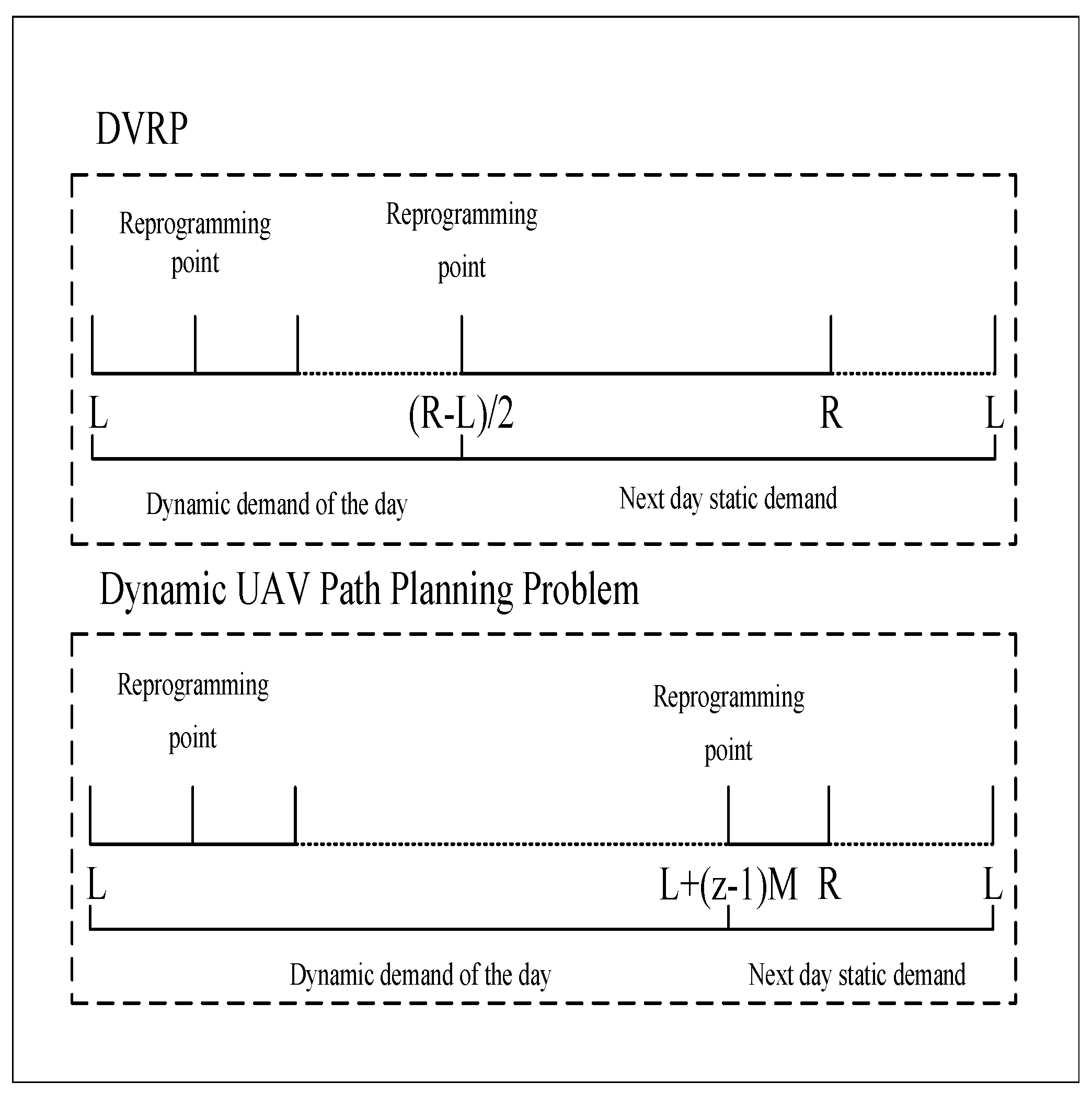
• We introduce the concept of time slicing, which accounts for the time-varying demand and wind, and then propose a two-phase logistics UAV path planning framework to address the dynamic customer demands through customer pool updates and kinetic attitude analysis. Based on this framework, the dynamic UAV path planning problem is transformed into a static problem at each time-slice node through initial pre-planning and subsequent delayed replanning. Then, a dynamic demand and wind-aware logistics UAV path planning problem is formulated to minimize the weighted average of the energy consumption cost and customer satisfaction penalty cost, while thoroughly considering constraints related to the energy consumption, load capacity, and hybrid time window.
• To address the issue of slow convergence and the tendency of the traditional PSO algorithm to fall into local optima, we incorporate an inferior solution mutation strategy. Specifically, a threshold is established, and when the number of successive iterations without the appearance of a superior individual exceeds this threshold, poorly-adapted particles within the swarm are reinitialized. Furthermore, we introduce the concept of selective crossover, commonly found in GA, into the traditional PSO algorithm. This approach allows for the “inheritance” of better values from certain dimensions retained from previous iterations, enabling newly generated particles to search for optimal positions based on these values. Consequently, we have an improved PSO-based multiple logistics UAV path planning algorithm to solve the formulated problem, which has a good performance with fast convergence and better solutions.
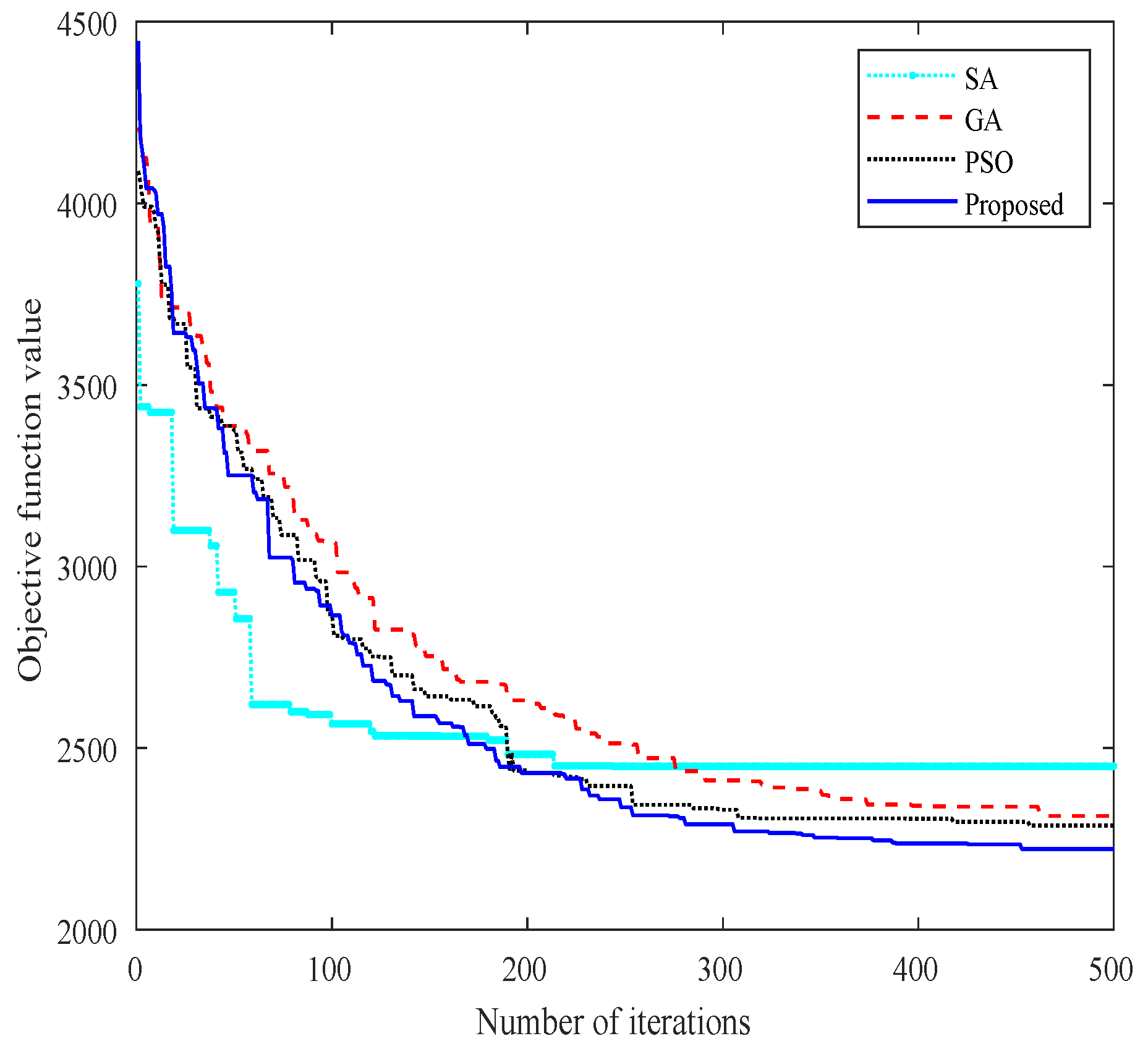
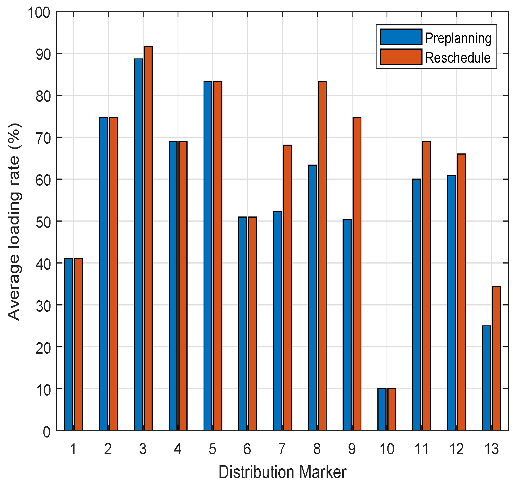
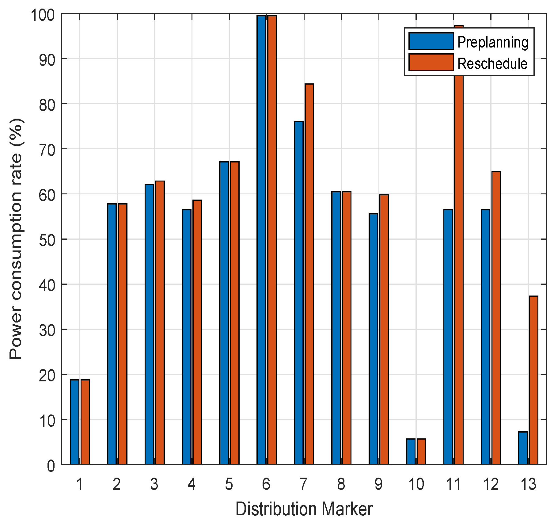
• To validate the advantages of the proposed algorithm, we utilize the Solomon-R201 dataset [41] for simulations, which is widely used as a standard benchmark dataset for testing and evaluating UAV delivery path planning algorithms. Wherein certain customer locations were randomized to represent new customer demands and alterations in existing customer information. Abundant simulation results verify that, when compared with the GA, simulated annealing (SA), and PSO-based UAV path planning strategies, the proposed algorithm achieves a satisfactory solution within a reasonable time and manages to reduce the distribution cost by up to $9.82$% amidst the dynamic customer demands and wind. Moreover, the average loading rate and battery consumption rate on the distribution paths, where the customer locations undergoing replanning are situated, are enhanced to $10.4$% and $15.75$%, respectively. This enhancement significantly boosts the loading efficiency and battery utilization rate during the UAV distribution, adhering to the constraints of the UAV’s maximum load and battery power.

The remainder of this work is structured as follows. In Section 2, we present the system model and then formulate the logistics UAV path planning problem. To solve this problem, the improved PSO-based multiple logistics UAV path planning algorithm is proposed in Section 3. Then, the advantages of the proposed algorithm are demonstrated in Section 4. Finally, we provide our conclusion and future work in Section 5.

2. System Model and Problem Formulation

In this section, we first provide the network model, and then, the dynamic customers’ demands and dynamic wind model are introduced. Based on this model, we develop a two-stage logistics UAV path planning framework that takes into account customer pool updates and dynamic attitudes. Subsequently, we formulate a dynamic demand and wind-aware logistics UAV path planning problem, aiming to minimize the weighted average of energy consumption and customer satisfaction penalty costs.

2.1. Network Model

As illustrated in Figure 1, we consider a logistics UAV distribution system that comprises multiple rechargeable multi-rotor UAVs with limited load capacities, capable of vertical takeoff and landing, along with a depot. After loading goods and replacing their batteries at the depot, the UAVs provide delivery and pickup services to the customers within the distribution range, according to the paths planned by the scheduling system. Throughout the distribution process, the variability in wind speed and direction and the dynamic changes in customer demands, including new and existing customer requests, are considered, which leads to dynamic adjustments in the distribution program. Firstly, the system pre-plans the distribution program based on the initial customer demand, continuously updating for new and modified demands, and deciding on their acceptance based on specific rules. Replanning occurs at various stages, taking into account the current progress of UAV deliveries and variables such as load and power. This process is repeated until all customer requirements are addressed. The main notations used in this work are shown in

Table 2. Notations and definitions.

Notations	Definitions
$\mathcal{C}$	The set of all nodes.
${\mathcal{C}}^s$	The set of nodes of the $s_{\mathrm{th}}$ time slice.
${\mathcal{C}}_0$	Depot.
${\mathcal{C}}_1^s$	Client locations waiting for further processing.
${\mathcal{C}}_2^s$	Client locations that have been processed.
${\mathcal{C}}_3^s$	A new need for a customer.
${\mathcal{C}}_4^s$	Client locations that meet time window constraints.
$g_i^s=\left(a_i^s,b_i^s\right)$	The coordinate of node i at time slice $s_{\mathrm{th}}$.
$di{s}_{ij}$	Distance from node i to node j at time slice $s_{\mathrm{th}}$.
$d_i^s$	Demand for deliveries at customer i.
$p_i^s$	Demand for pickup at customer i.
$l_i^s$	Earliest service window acceptable to customer i.
$r_i^s$	Latest service time window acceptable to customer i.
${\lambda }_1$	Penalty factor when UAV’s arrival time is earlier than the earliest acceptable service time window.
${\lambda }_2$	Penalty factor when UAV’s arrival time is later than the latest service time window.
L, R	The start and end times of the depot.
T	Depot working hours.
$\mathcal{S}={\left\{s^s\right\}}_{s=1}^z$	The set of time slices.
$\mathcal{T}={\left\{t^t\right\}}_{t=1}^v$	The set of wind speed and direction time sequences.
$h_{iu}^s$	Sum of descent, ascent and hovering time of UAV u at customer location i at time slice s.
$\mathcal{U}={\left\{u^u\right\}}_{u=1}^w$	The set of UAVs.
${\alpha }_{ij}^{st}$	Heading angle from node i to node j.
${\beta }_{ij}^{st}$	Trajectory angle from node i to node j.
$G{S}_{ij}^{st}$	Ground speed from node i to node j.
$Z_{ij}^{ut}$	Flight time from node i to node j.
$f_u$	Fixed costs of UAV u.
$m_{ij}^s$	The payload from node i to node j.
$ar{r}_{ij}^u$	Time for UAV u to arrive at node j from node i.
Q	The maximum payload of UAV.
$E_{max}$	The maximum power of UAV.
$e_{ij}^{su}$	Remaining power of UAV when it departs from node i to j.
$Z_{ij}^{sut}$	Flight time of UAV u from node i to node j in time slice s in time window t.
$\mathcal{X}=\left\{x_{ij}^{su}\right\}$	Binary variable to indicate whether the delivery service between node i and node j is performed by UAV u.
$\mathcal{Y}=\left\{y_{ij}^{su}\right\}$	Binary variable to indicate whether the UAV u performs the next delivery service again after returning to the depot.

.

The studies in this work are based on the following assumptions:

• It is assumed that the logistics UAVs depart from and subsequently return to the depot upon completing their pickup and delivery services. These UAVs execute battery replacements, as well as cargo loading and unloading tasks within the depot, in minimal time. In addition, these UAVs are uniform in type, and details regarding their loaded battery power and maximum payload capacity are precisely defined.
• Each customer’s pickup and delivery requirements are serviced by a single UAV during a singular instance. These requirements cannot be divided, ensuring the total weight remains within the UAV’s maximum payload capacity. Furthermore, each customer’s location is accurately identified and falls within the UAV’s operational delivery range.
• During the delivery tasks, the UAV maintains a constant airspeed, with wind speed and direction subject to time variations, impacting the entire delivery process and range. Foreknowledge of changes in wind speed and direction is assumed. It is presumed that, despite changes in wind patterns during cross-node flights or flights across different wind speed and direction time windows, the UAV maintains its trajectory by adjusting its heading, ignoring the potential time and errors associated with heading adjustments.

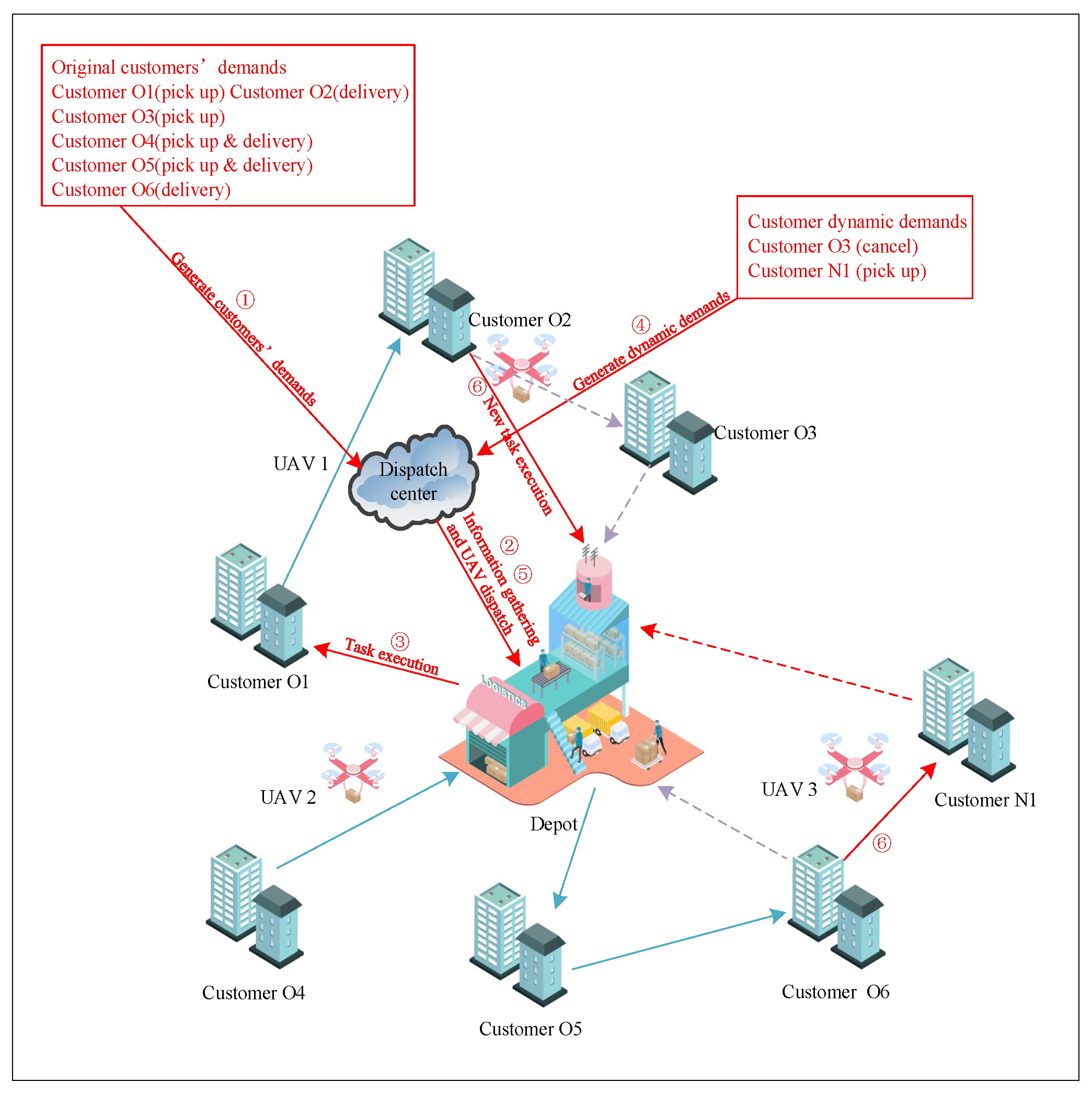
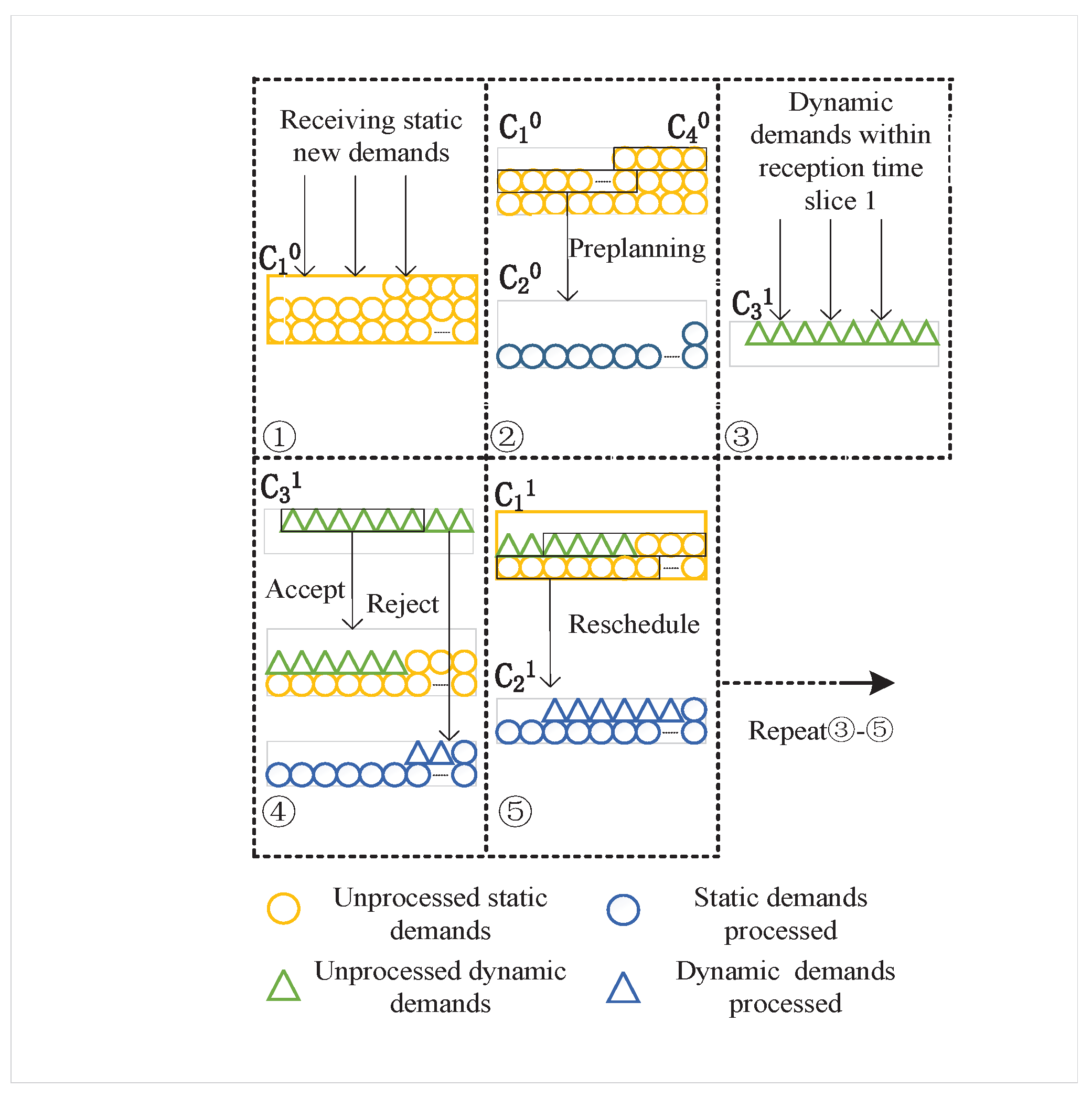
2.2. The Two-Phase Customer Demands Processing Model

During the logistics distribution process, the customer’s location information remains dynamic and cannot remain stable. When a new customer’s location emerges for the UAV in the logistics distribution process, the adjustments are necessary due to changes in the original customers’ demands and other dynamic factors. These adjustments involve reevaluating the planned distribution route. The dynamic demands from the customers significantly impact the task complexity of the logistics distribution system. Furthermore, the associated distribution task for the UAV undergoes modifications. The system’s efficiency depends on how effectively it responds to these dynamic customer demands, ultimately influencing distribution flexibility and customer satisfaction.

To cope with dynamic customer demands, two general processing methods are adopted: immediate and delayed processing. The immediate processing entails adding dynamic demands to the customer pool as soon as they arise and re-planning the distribution path based on new customer information. Although this method allows for timely response to new customer demands, frequent re-planning results in significant changes to delivery preparations. The delayed processing involves withholding dynamic demands from the customer pool until certain conditions are met for collective processing. These conditions typically encompass quantitative and timed processing approaches. Delayed quantitative processing waits until the customer’s demand changes reach a predefined threshold, at which location-accumulated demands are added to the customer pool for subsequent path re-planning. However, the interval before reaching this threshold can be prolonged, causing some dynamic demands to experience significant delays before being addressed. Delayed timed processing divides the depot’s operational hours into daily time segments, adding the accumulation of new customer demands to the pool at set intervals for path re-planning based on the updated pool. To mitigate excessive dynamic demand due to frequent path replanning and to prevent delays in processing customer demands during periods of low demand accumulation, which may not meet the processing threshold, we employ the delayed timed processing approach for managing dynamic customer demands.

To address the delayed timing processing, we incorporate the duration of working days into the timing strategy, leveraging periodic optimization to segment the depot’s operational hours into equal time slices. Customer demands prior to the depot’s operational window are considered initial static customer demands, and those within the operational window categorized as dynamic customer demands. Utilizing this approach, a two-phase logistics UAV path planning framework is proposed, which is shown in Figure 2. In this framework, it is assumed that the depot operates within a time window of $[L,R]$, and the timeframe is divided into N equal time slices, each with a duration of $(R-L)/N$. Prior to L, the path planning system continuously accumulates customer demands up to the time L. The initial static customer demands collected are pre-planned, with the logistics UAVs commencing deliveries based on these pre-planning results. During the task execution, the system dynamically accepts or rejects new customer demands within each time slice. Prior to concluding each time slice, the system re-plans the paths by integrating the current distribution plan with unserviced customer locations, transforming the dynamic path planning challenge into a static one within each time slice. This process is repeated for each time slice until the depot’s operations cease at the R time slot. Towards the end of each time slice, the presence of advanced commitment time (ACT) prevents the transfer of delivery tasks among UAVs. Consequently, the commitment made to UAVs during the task allocation remains deterministic and final. As a result, the UAVs currently executing tasks will persist in completing those tasks until the end of the time slice.

2.3. The Dynamic Customer Pool Model

As depicted in Figure 3, the customer pool is divided into the pending customer pool $C_1^s$ and the processed customers pool $\left[C_2^s\right]$, based on acceptance by the distribution system at time slice s and the status of pickup or delivery tasks. $C_1^s$ includes unprocessed customer locations and those newly accepted. $\left[C_2^s\right]$ comprises customer locations actively engaged in or having completed distribution tasks and newly rejected customer locations. During the replanning process, customer locations $C_4^s$ within current time slices meeting the earliest acceptable time window constraints are subject to replanning. Notably, the new customer demands are added to a new demand pool $C_3^s$ for assessment. If rejected, they’re moved to $C_2^s$, otherwise to $C_1^s$. In the delivery process, pending customer pools for each current time slice are updated accordingly. As the distribution advances, the current time slice for both pending and processed customer pools is continuously updated, and as each time slice elapses, customer locations in the pending pool $C_1^s$ meeting time window constraints transition to $C_4^s$ for inclusion in the replanning process.

2.4. The Customers’ Dynamic Attitude Model

Similarly to [42], the customer’s dynamic attitude refers to the ratio of customers with dynamic demands to all customers within a specific time slice. Factors influencing this dynamic attitude include the cutoff time for dynamic responses, the number of time slices, and the advanced commitment time. The dynamic response cutoff time defines the threshold beyond which the distribution system ceases to react to dynamic demand, with requests beyond this cutoff deferred to the next working day. Typically, in standard datasets, the cutoff time is set at half the working day’s length. The number of time slices influences the replanning frequency, with more slices enabling quicker responses to customer demand, yet longer slices can reduce distribution costs, necessitating a balance between responsiveness and cost. Advance commitment time applies to the UAVs’ already assigned tasks, indicating these tasks cannot be reassigned, ensuring task commitment certainty and finality. Within each time slice, the cumulative number of dynamic demand customers increases, elevating the dynamic attitude and altering the strategic dynamic response environment. A dynamic response with a lower dynamic attitude can swiftly meet customer demands but at the cost of increased distribution expenses; conversely, a higher dynamic attitude can cut distribution costs but may delay satisfying customer demands.

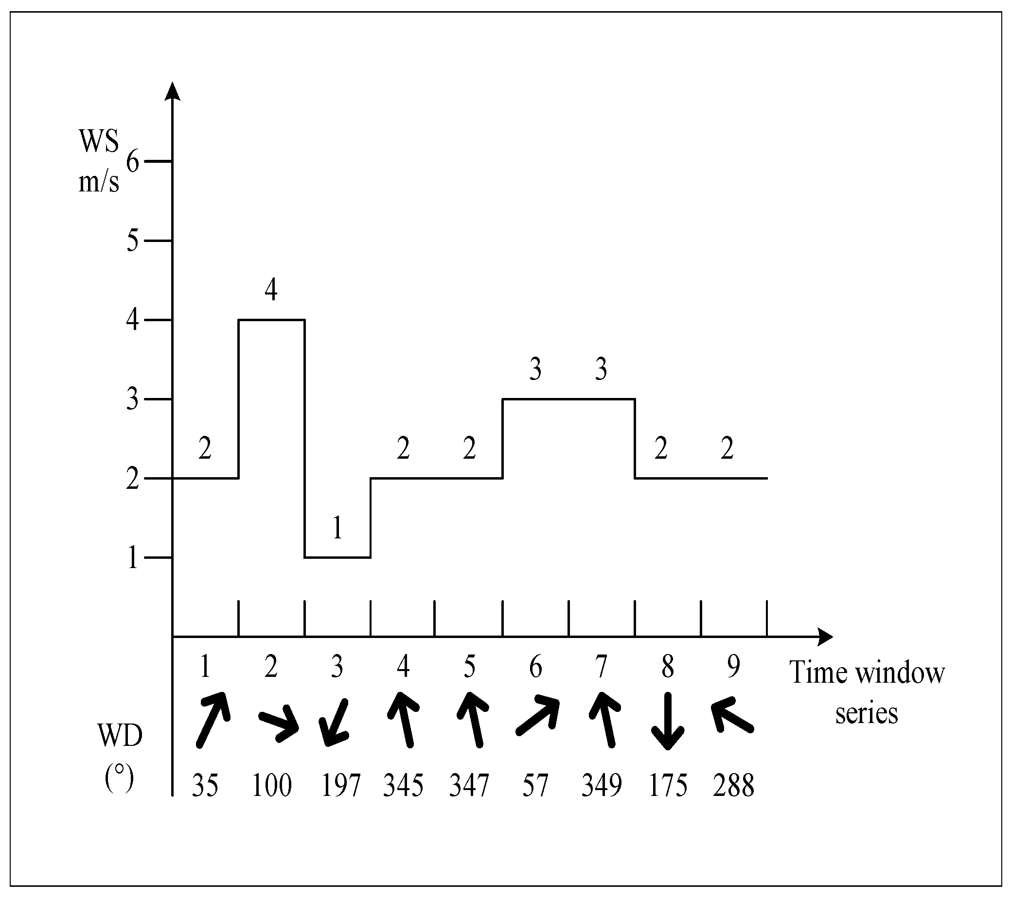
2.5. The Dynamic Wind Model

In the context of UAV logistics and distribution, the UAVs cannot consistently follow their expected flight paths due to the effects of airflow. For instance, tailwinds and headwinds alter delivery times between nodes, while crosswinds can cause deviations from the original flight trajectories, ultimately impacting the overall delivery route. The varying wind speeds and directions result in different degrees of influence. Therefore, in UAV logistics and distribution, the real-time adjustments for wind speed and direction changes are crucial.

As shown in [35], we discretize the dynamic wind speed and direction changes within the distribution area into distinct time windows, where wind conditions vary between windows, and assume a global influence of wind speed and direction across the entire UAV distribution range and process, with wind speed and direction for each time window anticipated in advance. Referencing the impact of wind speed and direction on logistics UAVs, as discussed in [43], to maintain stable airspeed and adhere to predetermined flight paths amid wind influences, the UAVs must first adjust their heading angles to counteract lateral wind deflections, subsequently adjusting ground speed as necessary to preserve airspeed following heading angle corrections. Building on these considerations, the following sections will further explore the logistics UAV path planning problem, taking into account dynamic customer demand and wind conditions.

2.6. The Degree of Dynamism

As shown in [42], the degree of dynamism in the logistics UAV path planning is the percentage of the number of dynamically demanding customers over all customers in a given time period during the course of the UAV’s delivery mission, i.e.,

$$\begin{array}{c}\hfill DoD={\displaystyle \frac{N_c^d}{N_c^d+N_c^s}}\times 100\%,\end{array}$$

(1)

where $N_c^d$ and $N_c^s$ denote the number of dynamic demand customers and the number of static demand customers in a time period, respectively.

In the classic dynamic vehicle routing problem (DVRP), with a depot working time window of $\left[L,R\right]$, the period is bisected by $\left(R-L\right)/2$ [44]. Customers requesting service before this midpoint are served the same day, whereas requests after are deferred to the next day. Customers requesting after $\left(R-L\right)/2$ on the previous day and before L on the current day are considered static, while those within $\left[L,\left.\left(R-L\right)/2\right)\right.$ of the current day are deemed dynamic. Considering the UAV delivery’s flexibility, this study segments the depot working time into equal-length slices, transforming the entire work period into Z equal consecutive intervals, each of duration $M=\left(R-L\right)/z$. As illustrated in Figure 4, the dynamic response cutoff is at the end of the penultimate time slice and treats customers with requests before L on the day following $L+\left(z-1\right)M$ as static and requests within $\left[L,\left.L+\left(z-1\right)M\right)\right.$ as dynamic for that day.

For dynamic customers arising within the $\left[L+\left(i-1\right)M,\left.L+iM\right)\right.$ time period of the day, the decision to accept a dynamic request is based on the following rules: for a new pickup/delivery demand within the time window $\left[l_k^i,\left.r_k^i\right)\right.$, accept the dynamic request if $r_k^i\ge L+\left(i-1\right)M$; otherwise, reject it. This rule also applies when the time window of an existing customer location changes dynamically, temporarily disregarding rejections due to changes in the pickup/delivery demands or location of existing customer locations.

Given that the dynamic customer demand imposes higher response rate requirements on the distribution system, to enhance the path planning stability, this paper introduces two dynamic demand replanning strategies, categorized by the level of motivational attitude. First, the motivational level is assessed based on the existing UAV fleet’s capability to timely complete the next time slice’s distribution tasks after accommodating dynamic demand. If the current UAV fleet can still meet the distribution timeline, this is classified as low motivation, prompting local adjustments to the distribution plan using a local optimization strategy. Should an increase in UAVs be necessary to adhere to the schedule, this constitutes a high motivational attitude, necessitating the use of a global optimization strategy for the replanning. This determination of motivational attitude, high or low, can be facilitated by establishing a threshold value.

2.7. Problem Formulation

In this work, we investigate the dynamic demand and wind-aware logistics UAV path planning problem to minimize the weighted average of the energy consumption cost and the customer satisfaction penalty cost, which takes the energy consumption constraints, load weight constraints, and hybrid time window constraints into account. Consequently, this dynamic logistics UAV path planning problem can be formulated as follows:

$$\begin{array}{ll}\underset{\mathcal{X},\mathcal{Y}}{min}{C}^T& =\sum _{u\in \mathcal{U}}\left\{{\kappa }_1·{\left(W+m_{ij}^s\right)}^{{\displaystyle \frac{3}{2}}}·\chi ·\left(\sum _{t=1}^k{Z}_{ij}^{ut}+h_{ju}^s\right)·x_{ij}^{su}\right.\\ & +{\kappa }_2·\left({\lambda }_1·max\left\{l_j^s-ar{r}_{ij}^u,0\right\}+{\lambda }_2·max\left\{ar{r}_{ij}^u-r_j^s,0\right\}\right)·x_{ij}^{su}\}\end{array}$$

(2)

$$\begin{array}{cc}\hfill & \mathrm{s}.\mathrm{t}.x_{ij}^{su}\in \{0,1\},i\in C_4^s,j\in C_4^s,u\in \mathcal{U},i\ne j,\hfill \end{array}$$

(3)

$$\begin{array}{cc}\hfill & y_{ij}^{su}\in \{0,1\},i\in C_4^s,j\in C_4^s,u\in \mathcal{U},i\ne j,\hfill \end{array}$$

(4)

$$\begin{array}{cc}\hfill & \sum _{u\in \mathcal{U}}\sum _{j\in C_s^{\prime }}{x}_{ij}^{su}=1,i\in C_4^s,\hfill \end{array}$$

(5)

$$\begin{array}{cc}\hfill & \sum _{i\in C_s^{\prime }}{x}_{ij}^{su}=\sum _{k\in C_s^{\prime }}{x}_{jk}^{su},u\in \mathcal{U},j\in C_4^s,i\ne j,\hfill \end{array}$$

(6)

$$\begin{array}{cc}\hfill & \sum _{j\in C_s^{\prime }}{y}_{ij}^{su}=x_{i0}^{su},i\in C_4^s,i\ne j,\hfill \end{array}$$

(7)

$$\begin{array}{cc}\hfill & \sum _{i\in C_4^s}{x}_{0j}^{su}-\sum _{{\displaystyle \genfrac{}{}{0pt}{}{i\in C_4^s,j\in C_4^s\hfill }{i\ne j\hfill }}}{y}_{ij}^{su}\le w,i\in C_4^s,u\in U,i\ne j\hfill \end{array}$$

(8)

$$\begin{array}{cc}\hfill & 0\le m_{ij}^s\le Q,i\in C_s^{\prime },j\in C_s^{\prime },i\ne j,\hfill \end{array}$$

(9)

$$\begin{array}{cc}\hfill & m_{ij}^s-m_{jk}^s=d_i^s-p_i^s,i\in C_s^{\prime },j\in C_4^s,k\in C_s^{\prime },i\ne j,j\ne k,\hfill \end{array}$$

(10)

$$\begin{array}{cc}\hfill & e_{0j}^{su}=E_{max}·x_{oj}^{su},j\in C_4^s,\hfill \end{array}$$

(11)

$$\begin{array}{cc}\hfill & 0\le e_{ij}^{su}\le E_{max},i\in C_4^s,j\in C_4^s,u\in \mathcal{U},i\ne j,\hfill \\ \hfill & e_{ij}^{su}-e_{jk}^{su}={\left(W+m_{ij}^s\right)}^{{\displaystyle \frac{3}{2}}}·\chi ·\left(\sum _{t=1}^k{Z}_{ij}^{ut}+h_j^{su}\right)·x_{ij}^{su},\hfill \end{array}$$

(12)

$$\begin{array}{cc}\hfill & i\in C_s^{\prime },j\in C_4^s,k\in C_s^{\prime },i\ne j\ne k,u\in \mathcal{U},t\in \mathcal{T},\hfill \end{array}$$

(13)

where the objective function $C^T$ of this problem is to minimize the distribution cost for each time slice, i.e.,  to minimize the weighted average of the energy consumption and the cost of customer satisfaction penalties. As shown in [26], the  energy consumption can be calculated by ${\left(W+m\right)}^{{\displaystyle \frac{3}{2}}}\sqrt{g^3/2\rho \zeta n}$, where W is the empty weight of the UAV, m is the actual load of the UAV, the value of $\chi =\sqrt{g^3/2\rho \zeta n}$ depends on the type of the UAV, g is the acceleration of gravity, $\rho$ is the air fluid density, $\zeta$ and n are the area of the rotor blades and the number of rotor blades, respectively. On the other hand, the cost of customer satisfaction penalties can be calculated based on the service time window model proposed in [45,46]. In addition, ${\kappa }_1$ and ${\kappa }_2$ represent the weights of energy consumption and the customer satisfaction penalty cost in the objective function, which serves as a trade-off between energy consumption and the customer satisfaction penalty cost, while they should satisfy the conditions ${\kappa }_1+{\kappa }_2=1,0\le {\kappa }_1\le 1,0\le {\kappa }_2\le 1$.

In this problem, constraints (3) and (4) define two decision variables: whether the UAV performs the delivery service between nodes in the first time slice and whether it executes the subsequent delivery task upon returning to the depot, respectively. Constraints (5) and (6) ensure a unique UAV is assigned to each customer location and that the UAV departs after completing its delivery task there. Constraint (7) ensures the UAV, after completing a delivery task and returning to the depot, can be reused for the next delivery task. Constraint (8) specifies that the number of UAVs operating at the same time slice must not surpass the total available UAVs in the system. Constraint (9) states that the UAV’s load weight at any node must always remain below its maximum weight limit. Constraint (10) describes the difference in UAV load weights before and after completing a delivery at a customer location as the disparity between delivery and pickup demands for that location. Constraints (11) and (12) ensure UAVs are fully charged upon departure from the depot and capable of prolonged flight. Constraint (13) represents the UAV’s power consumption during delivery tasks at neighboring nodes across varying wind speed and direction time windows.

3. Proposed Dynamic Demand and Wind-Aware Logistics UAV Path Planning Algorithm

In this section, we propose a dynamic demand and wind-aware logistics UAV path planning algorithm to cope with the dynamic customer demands and wind in logistics UAV distribution. More specifically, the dynamic-customers demand-driven UAV path planning problem is converted into a static problem across multiple time slices by utilizing the time-slicing strategy. Subsequently, we develop a pre-planning and delayed replanning combined UAV path planning algorithm to solve this static problem. During the preplanning phase, an improved PSO algorithm is utilized to facilitate the task planning for each time slice. While, during the delayed replanning phase, the global and local optimization strategies are developed to address the high and low dynamic demand scenarios, respectively, through the evaluation of demand dynamics in each time slice. For the global optimization, the same improved PSO algorithm from the pre-planning phase is utilized, while the local optimization strategy employs an insertion algorithm for adjustments to the original distribution plan.

3.1. The Description of Proposed Algorithm

As presented in Algorithm 1, we propose a dynamic demand and wind-aware logistics UAV path planning algorithm to cope with the dynamic customer demands and wind in logistics UAV distribution, which combines the pre-planning and delayed replanning outlined in the two-phase processing framework detailed previously. During the pre-planning phase, an improved PSO algorithm is utilized to facilitate the task planning for each time slice. During the delayed replanning phase, the global and local optimization strategies are developed to address the high and low dynamic demand scenarios, respectively, through the evaluation of demand dynamics in each time slice. For the global optimization, the same improved PSO algorithm from the pre-planning phase is utilized, while the local optimization strategy employs an insertion algorithm for adjustments to the original distribution plan.

Algorithm 1 Dynamic Demand and Wind-aware Logistics UAV Path Planning Algorithm

Input: The parameters of customer location, depot, wind speed and direction, and logistics UAVs. 1: Using the proposed improved PSO-based UAV path pre-planning algorithm (Algorithm 2) to obtain the pre-planned distribution routes. 2: if the customer demands have changed 3: Enter the change information of the customer demands. 4: Update the customer pool. 5: Employ the insertion algorithm to compute the objective function value. 6: end if 7: if the objective function value is less than the penalty factor set to be extremely positive 8: Employ the proposed insertion-based local optimization algorithm (Algorithm 3) to perform the local path planning. 9: else Employ the proposed, improved PSO-based UAV path pre-planning algorithm (Algorithm 2) for the global path replanning. 10: end if 11: Execution of planned distribution routes. 12: Repeat from step 2 until the end of time slicing. Output: The optimal logistics UAV distribution paths.

Specifically, for  customer location i requiring the insertion, it is sequentially inserted into sub-distribution paths, and the associated objective function value is calculated. Violations of UAV energy and loading constraints are quantified using the penalty factor $\varphi$, a value significantly larger than the objective function value. If the quantized objective function value is less than $\varphi$, it signifies a low-motivation case. This indicates that none of the current sub-distribution paths achieve an insertion point compliant with UAV energy and load constraints, necessitating global replanning for the high-motivation scenario.

3.2. The Improved PSO-Based UAV Path Pre-Planning Algorithm

Given that pre-planning and global replanning for high-mobility demand scenarios are largely analogous, the same algorithm is utilized for both to address the issue. As the formulated problem involves dynamic and real-time characteristics, the solution space changes dynamically with distribution, necessitating higher algorithm performance to enhance solution efficiency and avoid local optima. We propose an improved PSO-based UAV path pre-planning algorithm, which is detailed in Algorithm 2, incorporating an inferior solution mutation strategy into the traditional framework. This enables particles to escape the current search region and explore previously unexplored areas of the solution space, thus preventing premature convergence to local optima, and integrates selective crossover from the traditional GA to increase particle diversity and enhance the swarm’s solution-searching capabilities. The detailed steps of the improved PSO-based UAV path pre-planning algorithm are described as follows.

Algorithm 2 The Improved PSO-based UAV Path Pre-Planning Algorithm

Input: The parameters of the customer location, depot, wind speed and direction, logistics UAVs, particle swarm size NIND, maximum number of iterations GENmax, current number of iterations j, initial inertia weight $\omega$, inertia weight decay coefficient $\lambda$, cognitive coefficient $c1$, social coefficient $c2$, particle position upper limit $X_{max}$, lower particle position limit $X_{min}$, particle velocity upper limit $V_{max}$, particle velocity lower limit $V_{min}$, inferior solution mutation strategy threshold N. 1: Initialize the particle swarm. For each particle $i=1,2,\dots ,N$: Random initialization of position $z_i$ and velocity $v_i$ 2: Calculate the initial fitness value $f\left(z_i\right)$ for each particle. 3: Calculate individual optimization $p_{\mathrm{best}}^i=z_i$ and global optimization $g_{\mathrm{best}}$. 4: while  $j\le GENmax$  do 5:    for $i=1,2,\dots ,N$, 6:       Update velocity: $v_i=\omega v_i+c_1\alpha (p_{\mathrm{best}}^i-z_i)+c_2\beta (g_{\mathrm{best}}-z_i)$ 7:       Update position: $z_i=z_i+v_i$ 8:    end for 9:    Calculate the fitness of the new position: $f\left(z_i\right)$ 10:    if $f\left(z_i\right)\ge f\left(p_{\mathrm{best}}^i\right)$ 11:       Cross-preservation of the current iteration’s optimum, global optimum, and individual optimums. 12:       if there is a superior individual after crossover 13:          Update the position and velocity of each particle. 14:       end if 15:    else 16:       if the number of iterations that have not been updated reaches a threshold value N. 17:          Perform the poorly resolved mutation strategy. 18:       end if 19:    end if 20:    $j=j+1$ 21: end while Output: The optimal UAV distribution solutions during the path pre-planning process.

3.2.1. Encoding and Decoding Strategies

To cope with dynamic customer demands in the UAV path planning, we employ an encoding method for particle positions within the improved PSO algorithm. It is assumed to have N customer locations in the distribution system and U UAV sorties performing delivery tasks, and the particle positions are defined as a two-row matrix $[U_m;U_s]$. $U_m$, encoded as a natural number from 1 to U, denotes the number of UAV sorties serving the respective customer location. $U_s$, encoded as a real number between 1 and N, represents the service order of customer locations in each UAV sortie. When decoding a particle, customer locations are first categorized by UAV sortie number $U_m$, then ordered by $U_s$ according to these categories, with this sorting order determining the service sequence in the UAV deliveries.

The encoding and decoding process is illustrated through the following example. To aid understanding, the  depot is labeled 0, the 12 customer locations are sequentially labeled 1–12, and the four UAVs’ flights are labeled 1–4. Given a particle’s position matrix, as depicted in

Table 3. The particle position encoding situation.

Customer Location Label	${\mathit{U}}_{\mathit{m}}$ Marker	${\mathit{U}}_{\mathit{s}}$ Marker
1	4	1.17
2	1	3.34
3	3	6.56
4	2	11.49
5	3	1.89
6	1	5.82
7	4	9.60
8	3	10.98
9	2	7.87
10	4	8.14
11	2	4.71
12	1	2.05

, during decoding, since customer locations 2, 6, and 12 have $U_m$ labels of 1, they are all assigned to the 1st UAV for delivery. By comparing the $U_s$ labels of these locations, the service sequence is determined as 0-12-2-6-0 based on the $U_s$ values. Thus, the specific delivery scheme corresponding to the encoding strategy is presented in Table 3 and 

Table 4. The distribution scheme obtained after decoding.

UAV Flights	Distribution Program
1	0-12-2-6-0
2	0-11-9-4-0
3	0-5-3-8-0
4	0-1-10-7-0

.

3.2.2. Update of Particles

To ensure the algorithm initially performs a comprehensive global search of the solution space and transitions to a detailed local search in subsequent iterations, we developed a speed updating mechanism where the inertia weights $\omega$ decay exponentially, specifically, during the $t_{th}$ iteration.

$$\begin{array}{cc}\hfill & {\omega }_t={\displaystyle \frac{{\omega }_0}{{\lambda }^{1-t}}},\hfill \end{array}$$

(14)

$$\begin{array}{cc}\hfill & V_{ij}^{t+1}={\omega }_t{V}_{ij}^t+c_1\alpha \left(B_{ij}^t-Z_{ij}^t\right)+c_2\beta \left(B_{gj}^t-Z_{ij}^t\right),i=1,2,\dots ,n,\hfill \end{array}$$

(15)

$$\begin{array}{cc}\hfill & X_{ij}^{t+1}=X_{ij}^t+V_{ij}^t,i=1,2,\dots ,n,\hfill \end{array}$$

(16)

where ${\omega }_t$ is the inertia coefficient at the $t_{th}$ iteration, and  $\lambda$ is the inertia weight decay coefficient, a real number between $\left(0,1\right)$. As the number of iterations increases, ${\lambda }^{1-t}$ increases, and  ${\omega }_t$ decreases, ensuring strong global search capability at the iteration’s start, and progressively enhancing local search ability in the current region as iterations proceed, thus dynamically adjusting the search capabilities of the algorithm. Meanwhile, $V_{ij}^{t+1}$ and $X_{ij}^{t+1}$ denote the velocity and position of the $i_{th}$ particle in the $j_{th}$ dimension after the $t_{th}$ iteration, respectively; $B1$ and $B2$ represent the individual optimal value of the $i_{th}$ particle and the overall optimal value of the swarm at the $t_{th}$ iteration, respectively. $c_1$ and $c_2$ are the cognitive and social coefficients, representing the influence of a particle’s historical and swarm information, respectively, and $\alpha$ and $\beta$, random numbers uniformly distributed between $\left(0,1\right)$, are introduced to enhance the randomness in particle updates. Using the above formula, particles navigate the search space, learning from individual and social experiences to guide their search direction and step size, continually updating their position and velocity to find the optimal solution.

3.2.3. Calculation of Individual Fitness Values

Initially, the energy consumption of each UAV during actual task execution is calculated and the satisfaction penalty value for each customer location is determined based on the initially generated or perturbed delivery tasks. To address violations of the model constraints, we introduce highly positive penalty factors for quantization. These adjustments aim to resolve issues related to UAV energy consumption constraints and load constraints. Ultimately, we compute the objective function value of the current solution, considering the respective weights.

Once the objective function value for the current solution is obtained, its individual fitness is computed using a fitness function. This fitness value serves as an evaluation metric for the solution’s effectiveness and guides subsequent operations based on its magnitude. The goal of this section is to minimize the weighted average of energy costs during distribution and satisfaction penalties at customer locations, which can be expressed as

$$\begin{array}{cc}\hfill & \underset{\mathcal{X},\mathcal{Y}}{min}{C}^T=\sum _{u\in \mathcal{U}}\left\{{\kappa }_1·{\left(W+m_{ij}^s\right)}^{{\displaystyle \frac{3}{2}}}·\chi ·\left(\sum _{t=1}^k{Z}_{ij}^{ut}+h_{ju}^s\right)·x_{ij}^{su}\right.\hfill \\ \hfill & +{\kappa }_2·\left({\lambda }_1·max\left\{l_j^s-ar{r}_{ij}^u,0\right\}+{\lambda }_2·max\left\{ar{r}_{ij}^u-r_j^s,0\right\}\right)·x_{ij}^{su}\}.\hfill \end{array}$$

(17)

Consequently, the inverse of the objective function value is taken as the individual fitness, ensuring that higher fitness values correspond to smaller weighted averages.

3.2.4. The Mutation Strategy

To prevent the algorithm from stagnating at a local optimum during iterations, this study incorporates a cleavage mutation strategy into the traditional particle swarm optimization algorithm. Specifically, a threshold is set whereby, if a more optimal individual fails to emerge within a certain number of successive iterations exceeding this threshold, the poorly adapted particles within the current swarm undergo re-initialization. This approach aims to enhance the swarm’s exploration of the solution space, facilitating an escape from local optima and fostering a continued search for optimal solutions in subsequent iterations. For instance, if the swarm fails to generate improved particles for more than 10 consecutive generations, $10\%$ of the particles with suboptimal fitness values is reinitialized. This strategy allows them to escape local optima and facilitates their ongoing search for better solutions in subsequent iterations.

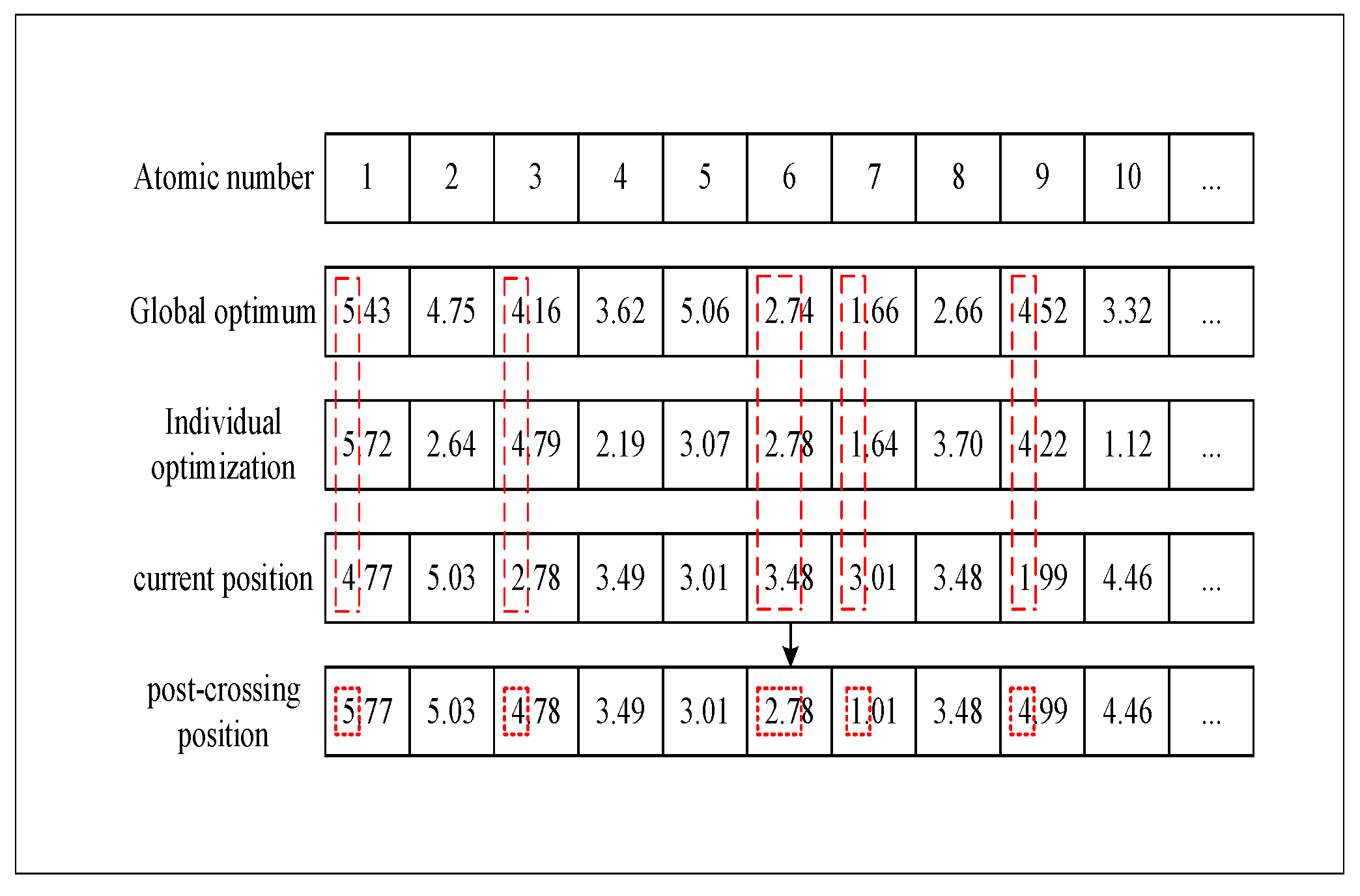
3.2.5. Selection of Cross-Cutting Strategy

Within a single iteration of the particle swarm algorithm, two types of optimal particles are identified: individual optimal particles and the global optimum of the entire swarm. To accelerate the convergence and “inherit” superior dimensional values from a previous iteration, enabling newly generated particles to find improved positions, we propose a selection crossover strategy based on a PSO algorithm. The specific selection process for crossover is illustrated in Figure 5, using the i-th particle in the t-th iteration as an example. For particle i, this includes the swarm’s global optimal position, particle i’s historical optimal position, and the position of the optimal particle in the t-th iteration; positions of these optimal particles are compared, retaining those with identical values corresponding to particle i. For instance, in Figure 5, the optimal value 5 of the iterated particle at ordinal number 1 is swapped with 4 of the current particle’s position, yielding the new particle position $5.77$, and values marked with dashed lines represent the dimensions’ optimal values retained from the previous iteration.

3.3. The Insertion-Based Local Optimization Algorithm

In the scenario where the customer dynamic demand is low, meaning the current system has enough UAVs to timely complete delivery tasks, we employ an insertion algorithm for local adjustments to the original delivery plan, which is detailed in Algorithm 3. Upon receiving the new customer’s demand, the system evaluates the existing UAV distribution task sequence, assessing whether each UAV’s remaining capacity and power can accommodate this new demand. For UAVs and sub-distribution sequences meeting the new demand, it sequentially evaluates the feasibility of inserting the new demand, calculating various potential insertion costs and selecting the insertion location with the lowest cost to distribute the new demand. Selecting the lowest-cost location for new demand insertion into the sub-distribution path is central to the scheduling strategy. Specifically, for each new demand at a customer location, the process involves traversing generated sub-distribution paths, sequentially inserting the customer location, and calculating the current objective function value. Violations of the UAVs’ energy consumption and load constraints during insertion are quantified using a penalization factor. Ultimately, the customer location is inserted at the position with the smallest objective function value, thereby integrating it into the distribution path. If, upon traversing the entire sub-distribution path, no suitable insertion location meeting the UAV’s energy and load constraints is found, global replanning is initiated based on a high-mobility strategy.

Algorithm 3 The Insertion-based Local Optimization Algorithm

Input: Distribution sequence $\mathcal{S}$ in place, the set of client locations to be inserted $\mathcal{U}$. 1: while $\mathcal{U}$ is not empty 2:    for each location i in $\mathcal{U}$ 3:       Calculate the objective function of the sub-distribution sequence for location i 4:    end for 5:     Select the location with the smallest objective function value for current location insertion. Insert customer location i into the sub-distribution sequence $\mathcal{S}$. 6:    Remove client location i from set $\mathcal{U}$. 7: end while Output: The optimal distribution solutions.

3.4. The Analysis of Time Complexity

As shown in [47,48], the time complexity of the PSO algorithm is $O(N\ast M)$, where N denotes the number of particles, and M represents the number of iterations. In accordance with Algorithm 1, when inserting a customer location “i”, it is sequentially placed within various sub-delivery paths, and the corresponding objective function values are computed. The penalty factor $\varphi$ quantifies the violation of UAV energy and load constraints, significantly surpassing the objective function value. If the quantized objective function value falls below $\varphi$, it signifies a low-motivation scenario, indicating that no existing sub-distribution path can accommodate the insertion location while adhering to UAV energy and load constraints. In cases with high dynamic demands, global replanning becomes imperative. For each new customer location requiring insertion, the algorithm iterates through all generated sub-delivery paths, evaluating the objective function value to determine the optimal placement. The proposed algorithm’s time complexity primarily hinges on the PSO algorithm. Consequently, the overall time complexity of the proposed algorithm is $O(m\ast n)$, where m represents the number of customer locations to be inserted, and n denotes the number of sub-delivery paths.

4. Simulation Results

In this section, we conduct extensive numerical simulations to validate the advantages of the proposed algorithm.

4.1. Simulation Scenario and Parameters Description

The numerical simulation of this work is conducted within a scenario that consists of a depot, 50 customer locations, and 4 ARK-150 UAVs. The length of the simulation scenario is 2500 m and the width is 2000 m. There is a distribution of 50 customer locations, each with specific pickup/delivery demands and service time windows. In addition, the depot is located at $(1050,1050)$ to incorporate four UAVs for serving these customer locations.

Similarly to [43], the ARK-150 hexacopter UAV is employed for logistics distribution in this work, with its specific parameters detailed in

Table 5. The parameters of UAV ARK-150.

Parameters	Value
Empty weight	100 kg
Maximum payload	30 kg
Maximum charge	1600 Wh
TAS	20 m/s

. These UAVs are loaded with goods and have their batteries replaced at the depot before servicing each customer location according to the paths planned by the scheduling system. Throughout the logistics distribution process, the impact of dynamic wind speed and direction, which is illustrated in Figure 6, is considered. To obtain the practical data on dynamic customer demands and wind, the R201 dataset from the Solomon series will be utilized for simulation and analysis [49,50]. This dataset will be suitably adjusted to accommodate the flexibility of UAV distribution, with 10 customers designated as those presenting dynamic demands. Moreover, the dynamic changes in customer demand, as detailed in

Table 6. System parameters for numerical simulation.

Parameter	Parameter Symbol	Value
Particle swarm size	$NIND$	500
Maximum number of iterations	$GE{N}_{max}$	500
Initial inertia weight	$\omega$	1
Inertia weight decay coefficient	$\lambda$	0.95
Cognitive coefficient	$c_1$	1.5
Social coefficient	$c_2$	2
Particle position upper limit	$X_{max}$	4
Lower particle position limit	$X_{min}$	1
Particle velocity upper limit	$V_{max}$	50
Particle velocity lower limit	$V_{min}$	−50
Inferior solution mutation strategy threshold	N	10

and

Table 7. The distribution sequences of the UAVs.

Distribution Serial Number	Distribution Sequence	Average Loading Rate	Electricity Consumption
1-1	0→26→40→0	41.11%	302
1-2	0→33→9 →29→3	76.67%	924.6
1-3	0→39→23→41 →53→22→0	88.67%	993.39
1-4	0→21→4→25 →24→12→0	68.89%	905.5
2-1	0→37→14→17 →45→18→0	83.33%	1073.9
2-2	0→46→47→11 →36→49→8→0	50.95%	1592.6
2-3	0→34→35→20 →32→50→57→0	52.22%	1217
3-1	0→1→30→10 →19→31→0	63.33%	968.32
3-2	0→6→42→15 →43→2→56→0	63.89%	889.49
3-3	0→27→0	10%	90.09
4-1	0→48→7→5 →13→51→0	60%	904.38
4-2	0→38→44 →16→52→0	60.83%	905.51
4-3	0→28→54→0	25%	114.81

, are also considered in the simulation to quantify the impact of dynamic customer demands on the logistics UAV distribution, and demonstrate the effectiveness of the proposed algorithm. The settings of some other parameters during the numerical simulation are shown in

Table 8. Information on the new customer demands.

Label	Type	a	b	Time	l	r	d	p
51	pickup	630	720	5	9	115	0	9
52		1470	1740	164	174	227	0	5
53		1110	930	172	207	245	0	3
54	delivery	360	720	102	145	189	7	0
55		1590	360	261	293	346	3	0
56	both	810	1290	67	87	150	6	3
57		1350	1960	296	361	431	4	7

.

4.2. Simulation Results Analysis

Figure 7 presents the convergence comparison graphs after 500 iterations of pre-planning the R201-50 dataset using the SA, GA, PSO, and proposed algorithm, respectively. It is observed that the objective function values of these four algorithms are $2450.01$, $2313.36$, $2287.40$, and $2222.59$, respectively. The objective function of the proposed algorithm shows a maximum reduction of about $9.28\%$, which highlights the proposed algorithm’s superior efficacy in distribution path pre-planning. Furthermore, the proposed algorithm’s ability to escape local optima underscores its capability to generate superior distribution solutions compared to the other three algorithms. Figure 8 displays the optimal path planning graph for the R201-50 dataset, as derived from the proposed algorithm, with the corresponding delivery sequences for each UAV and their analyses presented in

Table 9. The change information regarding existing customers.

Label	Type	a	b	Time	l	r	d	p
28	(l,r)	1230	1110	213	320	421	7	7
41	(a,b)	1260	210	103	198	255	10	7
50	(d,p)	1410	1410	67	274	321	6	9

.

Reflecting on the new customer requirements derived from pre-planning results, as depicted in Table 5, these requirements are organized by the sequence of customer submissions and the specific type of pickup and delivery requested. This includes detailing the location of customer locations with dynamic needs, the volume of pickup and delivery requests, their time windows, and the submission times of these dynamic requests. Furthermore, Table 6 presents changes to original customer data, with initial demands indicated in parentheses. In scenario R201-50, the depot’s operational hours are set from 0 to 500, according to the previously mentioned concept of time slicing, this timeframe is divided into five equal time slices, meaning that, from the onset of operations, each period is segmented into five slices to accommodate customer dynamic demand. The UAV delivery path undergoes replanning through either a local or global optimization strategy.

By integrating the new customer demand data from Table 6 with the original customer change information in Table 7, it is revealed that, at the 100-min mark of the depot’s operational hours, two new customer demands for No. 51 and No. 58 emerge, along with a change in demand for customer location No. 50. Following the demand change for customer location No. 50, the 2-3 delivery sequence remains within the UAV’s load and energy consumption limits, altering the average loading rate of the 2-3 delivery sequence to $69.44\%$ and the power consumption to 1283. The new customer demand No. 51 represents a pure pickup request, enabling its addition to the ongoing delivery sequence, guided by the minimum inserted objective function value, No. 51, followed by No. 58, can be incorporated into the current delivery sequence. Consequently, customer location No. 51 is integrated into the 4-1 distribution sequence, resulting in an average loading rate of $63.89\%$ for this sequence, with power consumption reaching $2593.2$. Assuming No. 58 involves simultaneous pickup and delivery, it necessitates insertion into a subsequent stage of the distribution path, and after evaluation, is inserted into the 3-2 distribution sequence, with an updated average loading rate of $74.76\%$ and power consumption of $2015.18$. In addition,

Table 10. The new distribution sequences of the UAVs after the customer demands change.

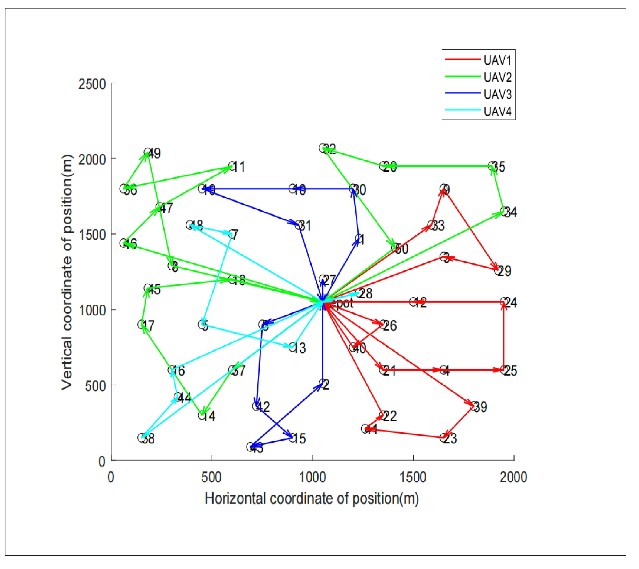
UAV Serial Number	Distribution Serial Number	Distribution Sequence
1	1-1	0→26→40→0
	1-2	0→33→9→29→3
	1-3	039→23→41 →53→22→0
	1-4	0→21→4→ 25→24→12→0
2	2-1	0→37→14 →17→45→18→0
	2-2	0→46→47→ 11→36→49→8→0
	2-3	0→34→35→20 →32→50→57→0
3	3-1	0→1→30→ 10→19→31→0
	3-2	0→6→42→ 15→43→2→56→0
	3-3	0→27→0
4	4-1	0→48→7→ 5→13→51→0
	4-2	0→38→44→ 16→52→0
	4-3	0→28→54→0

presents the final distribution sequence achieved via the optimization strategy, with all user demands met except for customer location 55, which is unable to be serviced due to time window constraints. This indicates the strategy and algorithm’s ability to address dynamic customer demands promptly and effectively.

Figure 9 and Figure 10 compare the average loading rate and battery consumption rate between the final and pre-planned distribution sequences, respectively. Based on distribution markers 1–13, as detailed in Table 10, it is evident that the average loading rate for distribution paths involving re-planned customer locations improved by an average of $10.4\%$, with a peak improvement of $24.36\%$. Furthermore, as depicted in Figure 10, the ARK-150’s maximum battery capacity is 1600 Wh. When comparing battery utilization before and after pre-planning and re-planning, the average increase in battery utilization across the aforementioned distribution sequences is $15.75\%$, equivalent to 252 Wh. Notably, distribution sequence 7 exhibits a remarkable $40.78\%$ increase in utilization. Thus, it can be concluded that UAV path planning, which accounts for dynamic customer demand, significantly enhances loading efficiency and battery utilization during delivery, adhering to the maximum UAV’s load and battery power constraints.

5. Conclusions and Future Work

In this work, we have investigated the dynamic demand and wind-aware logistics UAV path planning problem in intelligent transportation systems. To enhance the distribution system’s responsiveness to the dynamic customer demands and wind, we have introduced the concept of time slicing and developed a two-phase logistics UAV path planning framework based on customer pool updates and demand dynamics analysis. Based on this framework, we have formulated a logistics UAV path planning problem to minimize the weighted average of the energy consumption cost and the customer satisfaction penalty cost, which is subject to the energy consumption constraints, load weight constraints, and hybrid time window constraints. Through the pre-planning and delayed replanning, the dynamic logistics UAV path planning problem has been transformed into a static problem at each time slice. To solve this problem, we proposed an improved PSO-based multiple logistics UAV path planning algorithm. Then, we conducted an abundant numerical simulation to verify that the proposed algorithm achieves satisfactory solutions within a reasonable time for dynamic customer demands and wind. Moreover, it can be demonstrated that the proposed algorithm effectively enhances the loading efficiency and battery utilization during the UAVs’ delivery process, adhering to the UAVs’ maximum load and battery power constraints.

Based on the findings of our work and its limitations, future research will mainly focus on the following two aspects: on the one hand, in terms of modeling, the introduction of multiple depots within the region will be considered, expanding the model to include a broader range of weather conditions, particularly focusing on more precise variations in wind speed and direction. On the other hand, in real urban distribution scenarios, factors such as building heights, take-off and landing site locations, and charging station placements will be investigated for their effects on the cost and efficiency of the logistics UAVs. This will involve refining the modeling of the UAV path planning problem to incorporate these factors. Additionally, the feasibility and effectiveness of deep reinforcement learning algorithms will be explored.

References

- Ding, Y.; Jin, M.; Li, S.; Feng, D. Smart Logistics Based on the Internet of Things Technology: An Overview. Int. J. Logist. Res. Appl. 2021, 24, 323–345. [Google Scholar] [CrossRef]
- Feng, B.; Ye, Q. Operations Management of Smart Logistics: A Literature Review and Future Research. Front. Eng. Manag. 2021, 8, 344–355. [Google Scholar] [CrossRef]
- Aliahmadi, A.; Nozari, H.; Ghahremani-Nahr, J. Big Data IoT-based Agile-lean Logistic in Pharmaceutical Industries. Int. J. Innov. Manag. Econ. Soc. Sci. 2022, 2, 70–81. [Google Scholar] [CrossRef]
- Li, X.; Gong, L.; Jiang, F.; Shi, W.; Fan, L.; Gao, H.; Li, R.; Xu, J. Solving the Last Mile Problem in Logistics: A Mobile Edge Computing and Blockchain-Based Unmanned Aerial Vehicle Delivery System. Concurr. Comput. Pract. Exp. 2022, 34, e6068. [Google Scholar] [CrossRef]
- Jones, W.D. Amazon Plans to Take Home Delivery to New Heights. IEEE Spectr. 2023, 60, 16–17. [Google Scholar] [CrossRef]
- Yigit, K.A.; Dalkiran, A.; Karakoc, T.H. Applications of Drones in the Health Industry. In Unmanned Aerial Vehicle Design and Technology; Springer: Cham, Switzerland, 2023; pp. 69–93. Available online: https://link.springer.com/chapter/10.1007/978-3-031-45321-2_5 (accessed on 25 May 2024).
- Baloch, G.; Gzara, F. Strategic Network Design for Parcel Delivery with Drones under Competition. Transp. Sci. 2020, 54, 204–228. [Google Scholar] [CrossRef]
- Agatz, N.; Bouman, P.; Schmidt, M. Optimization Approaches for the Traveling Salesman Problem with Drone. Transp. Sci. 2018, 52, 965–981. [Google Scholar] [CrossRef]
- Chiang, W.C.; Li, Y.; Shang, J.; Urban, T.L. Impact of Drone Delivery on Sustainability and Cost: Realizing the UAV Potential through Vehicle Routing Optimization. Appl. Energy 2019, 242, 1164–1175. [Google Scholar] [CrossRef]
- Wu, Y.; Low, K.H. An Adaptive Path Replanning Method for Coordinated Operations of Drone in Dynamic Urban Environments. IEEE Syst. J. 2020, 15, 4600–4611. [Google Scholar] [CrossRef]
- Campuzano, G.; Lalla-Ruiz, E.; Mes, M. The Dynamic Drone Scheduling Delivery Problem. In International Conference on Computational Logistics; Springer International Publishing: Cham, Switzerland, 2022; pp. 260–274. Available online: https://springer.longhoe.net/chapter/10.1007/978-3-031-16579-5_18 (accessed on 25 May 2024).
- Sawadsitang, S.; Niyato, D.; Tan, P.S.; Wang, P.; Nutanong, S. Shipper Cooperation in Stochastic Drone Delivery: A Dynamic Bayesian Game Approach. IEEE Trans. Veh. Technol. 2021, 70, 7437–7452. [Google Scholar] [CrossRef]
- Khamidehi, B.; Raeis, M.; Sousa, E.S. Dynamic Resource Management for Providing QoS in Drone Delivery Systems. In Proceedings of the 2022 IEEE 25th International Conference on Intelligent Transportation Systems (ITSC), Macau, China, 8–12 October 2022; pp. 3529–3536. Available online: https://ieeexplore.ieee.org/abstract/document/9922133 (accessed on 25 May 2024).
- Khanda, A.; Coro, F.; Das, S.K. Drone-Truck Cooperated Delivery under Time Varying Dynamics. In Proceedings of the 2022 Workshop on Advanced Tools, Programming Languages, and PLatforms for Implementing and Evaluating Algorithms for Distributed Systems, Salerno, Italy, 25 July 2022; Association for Computing Machinery: New York, NY, USA, 2022; pp. 24–29. [Google Scholar] [CrossRef]
- Sorbelli, F.B.; Corò, F.; Das, S.K.; Pinotti, C.M. Energy-Constrained Delivery of Goods with UAVs under Varying Wind Conditions. IEEE Trans. Intell. Transp. Syst. 2020, 22, 6048–6060. [Google Scholar] [CrossRef]
- Han, J.; Liu, Y.; Li, Y. Vehicle Routing Problem with UAVs Considering Time Windows and Dynamic Demand. Appl. Sci. 2023, 13, 13086. [Google Scholar] [CrossRef]
- Liu, Y. An Optimization-Driven Dynamic Vehicle Routing Algorithm for on-Demand Meal Delivery using UAVs. Comput. Oper. Res. 2019, 111, 1–20. [Google Scholar] [CrossRef]
- Glick, T.B.; Figliozzi, M.A.; Unnikrishnan, A. Case Study of Drone Delivery Reliability for Time-Sensitive Medical Supplies with Stochastic Demand and Meteorological Conditions. Transp. Res. Rec. 2022, 2676, 242–255. [Google Scholar] [CrossRef]
- Zhang, J.; Campbell, J.F.; Sweeney, D.C., II; Hupman, A.C. Energy Consumption Models for Delivery UAVs: A Comparison and Assessment. Transp. Res. Part Transp. Environ. 2021, 90, 102668. [Google Scholar] [CrossRef]
- Xu, J.; Liu, X.; Li, X.; Zhang, L.; Jin, J.; Yang, Y. Energy-Aware Computation Management Strategy for Smart Logistic System with MEC. IEEE Internet Things J. 2021, 9, 8544–8559. [Google Scholar] [CrossRef]
- Huang, H.; Hu, C.; Zhu, J.; Wu, M.; Malekian, R. Stochastic Task Scheduling in UAV-Based Intelligent on-Demand Meal Delivery System. IEEE Trans. Intell. Transp. Syst. 2021, 23, 13040–13054. [Google Scholar] [CrossRef]
- Huang, C.; Ming, Z.; Huang, H. Drone Stations-Aided Beyond-Battery-Lifetime Flight Planning for Parcel Delivery. IEEE Trans. Autom. Sci. Eng. 2022, 20, 2294–2304. [Google Scholar] [CrossRef]
- Cherif, N.; Jaafar, W.; Yanikomeroglu, H.; Yongacoglu, A. Disconnectivity-Aware Energy-Efficient Cargo-UAV Trajectory Planning with Minimum Handoffs. In Proceedings of the ICC 2021-IEEE International Conference on Communications, Montreal, QC, Canada, 14–23 June 2021; pp. 1–6. [Google Scholar] [CrossRef]
- Liu, Z.; Sengupta, R.; Kurzhanskiy, A. A Power Consumption Model for Multi-Rotor Small, Unmanned Aircraft Systems. In Proceedings of the 2017 International Conference on Unmanned Aircraft Systems (ICUAS), Miami, FL, USA, 13–16 June 2017; pp. 310–315. [Google Scholar]
- Dorling, K.; Heinrichs, J.; Messier, G.G.; Magierowski, S. Vehicle Routing Problems for Drone Delivery. IEEE Trans. Syst. Man Cybern. Syst. 2016, 47, 70–85. [Google Scholar] [CrossRef]
- Abeywickrama, H.V.; Jayawickrama, B.A.; He, Y.; Dutkiewicz, E. Comprehensive Energy Consumption Model for Unmanned Aerial Vehicles, Based on Empirical Studies of Battery Performance. IEEE Access 2018, 6, 58383–58394. [Google Scholar] [CrossRef]
- Cheng, C.; Adulyasak, Y.; Rousseau, L.M. Drone Routing with Energy Function: Formulation and Exact Algorithm. Transp. Res. Part B Methodol. 2020, 139, 364–387. [Google Scholar] [CrossRef]
- Chen, Y.; Baek, D.; Bocca, A.; Macii, A.; Macii, E.; Poncino, M. A Case for a Battery-aware Model of Drone Energy Consumption. In Proceedings of the 2018 IEEE International Telecommunications Energy Conference (INTELEC), Turino, Italy, 7–11 October 2018; pp. 1–8. [Google Scholar]
- Funabashi, Y.; Taniguchi, I.; Tomiyama, H. Work-in-progress: Routing of Delivery UAVs with Load-Dependent Flight Speed. In Proceedings of the 2019 IEEE Real-Time Systems Symposium (RTSS), Hong Kong, China, 3–6 December 2019; pp. 520–523. [Google Scholar]
- Ito, S.; Akaiwa, K.; Funabashi, Y.; Nishikawa, H.; Kong, X.; Taniguchi, I.; Tomiyama, H. Load and Wind Aware Routing of Delivery UAVs. UAVs 2022, 6, 50. [Google Scholar]
- Sorbelli, F.B.; Corò, F.; Palazzetti, L.; Pinotti, C.M.; Rigoni, G. How the Wind Can be Leveraged for Saving Energy in a Truck-Drone Delivery System. IEEE Trans. Intell. Transp. Syst. 2023, 24, 4038–4049. [Google Scholar] [CrossRef]
- Cheng, C.; Adulyasak, Y.; Rousseau, L.M. Robust Drone Delivery with Weather Information. History 2020, 26, 1189–1585. [Google Scholar] [CrossRef]
- Radzki, G.; Thibbotuwawa, A.; Bocewicz, G. UAVs Flight Routes Optimization in Changing Weather Conditions—Constraint Programming Approach. Appl. Comput. Sci. 2019, 15, 5–12. [Google Scholar] [CrossRef]
- Hamdi, A.; Salim, F.D.; Kim, D.Y.; Neiat, A.G.; Bouguettaya, A. Drone-as-a-Service Composition under Uncertainty. IEEE Trans. Serv. Comput. 2021, 15, 2685–2698. [Google Scholar] [CrossRef]
- Peng, L.; Murray, C. Parallel Drone Scheduling Traveling Salesman Problem with Weather Impacts. Available at SSRN 4254262 2022. [Google Scholar] [CrossRef]
- Das, D.N.; Sewani, R.; Wang, J. Synchronized Truck and Drone Routing in Package Delivery Logistics. IEEE Trans. Intell. Transp. Syst. 2020, 22, 5772–5782. [Google Scholar] [CrossRef]
- Tong, B.; Wang, J.; Wang, X.; Zhou, F.; Mao, X.; Zheng, W. Optimal Route Planning for Truck–Drone Delivery using Variable Neighborhood Tabu Search Algorithm. Appl. Sci. 2022, 12, 529. [Google Scholar] [CrossRef]
- Hong, F.; Wu, G.; Luo, Q.; Liu, H.; Fang, X.; Pedrycz, W. Logistics in the sky: A Two-Phase Optimization Approach for the Drone Package Pickup and Delivery System. IEEE Trans. Intell. Transp. Syst. 2023, 24, 9175–9190. [Google Scholar] [CrossRef]
- Meng, Q.; Chen, K.; Qu, Q. PPSwarm: Multi-UAV Path Planning Based on Hybrid PSO in Complex Scenarios. Drones 2024, 8, 192. [Google Scholar] [CrossRef]
- Sajid, M.; Mittal, H.; Pare, S.; Prasad, M. Routing and Scheduling Optimization for UAV Assisted Delivery System: A Hybrid Approach. Appl. Soft Comput. 2022, 126, 109225. [Google Scholar] [CrossRef]
- Solomon, M.M. Algorithms for the Vehicle Routing and Scheduling Problems with Time Window Constraints. Oper. Res. 1987, 35, 254–265. [Google Scholar] [CrossRef]
- Okulewicz, M.; Mandziuk, J. A Metaheuristic Approach to Solve Dynamic Vehicle Routing Problem in Continuous Search Space. Swarm Evol. Comput. 2019, 48, 44–61. [Google Scholar] [CrossRef]
- Du, P.; Shi, Y.; Cao, H.; Garg, S.; Alrashoud, M.; Shukla, P.K. AI-Enabled Trajectory Optimization of Logistics UAVs with Wind Impacts in Smart Cities. IEEE Trans. Consum. Electron. 2024, 70, 3885–3897. [Google Scholar] [CrossRef]
- Bouleft, Y.; Elhilali Alaoui, A. Dynamic Multi-Compartment Vehicle Routing Problem for Smart Waste Collection. Appl. Syst. Innov. 2023, 6, 30. [Google Scholar] [CrossRef]
- Khan, R.; Tausif, S.; Malik, A.J. Consumer Acceptance of Delivery Drones in Urban Areas. Int. J. Consum. Stud. 2019, 43, 87–101. [Google Scholar] [CrossRef]
- Felch, V.; Karl, D.; Asdecker, B.; Niedermaier, A.; Sucky, E. Reconfiguration of the Last Mile: Consumer Acceptance of Alternative Delivery Concepts. In Logistics Management: Strategies and Instruments for Digitalizing and Decarbonizing Dupply Chains-Proceedings of the German Academic Association for Business Research, Halle, 2019; Springer International Publishing: Cham, Switzerland, 2019; pp. 157–171. [Google Scholar] [CrossRef]
- Bi, J.; Yuan, H.; Duanmu, S.; Zhou, M.; Abusorrah, A. Energy-Optimized Partial Computation Offloading in Mobile-Edge Computing with Genetic Simulated-Annealing-Based Particle Swarm Optimization. IEEE Internet Things J. 2020, 8, 3774–3785. [Google Scholar] [CrossRef]
- Asif, M.; Khan, M.A.; Abbas, S.; Saleem, M. Analysis of Space & Time Complexity with PSO Based Synchronous MC-CDMA System. In Proceedings of the 2019 2nd International Conference on Computing, Mathematics and Engineering Technologies, Sukkur, Pakistan, 30–31 January 2019; pp. 1–5. [Google Scholar] [CrossRef]
- The Data Set of Solomn. Available online: http://web.cba.neu.edu/~msolomon/problems.htm (accessed on 25 May 2024).
- Du, P.; He, X.; Cao, H.; Garg, S.; Kaddoum, G.; Hassan, M.M. AI-Based Energy-Efficient Path Planning of Multiple Logistics UAVs in Intelligent Transportation Systems. Comput. Commun. 2023, 207, 46–55. [Google Scholar] [CrossRef]