
Fast Finite-Time Super-Twisting Sliding Mode Control with an Extended State Higher-Order Sliding Mode Observer for UUV Trajectory Tracking


Abstract
1. Introduction
2. Uuv Modeling and Problem Formulation
2.1. Notations
2.2. Lemmas
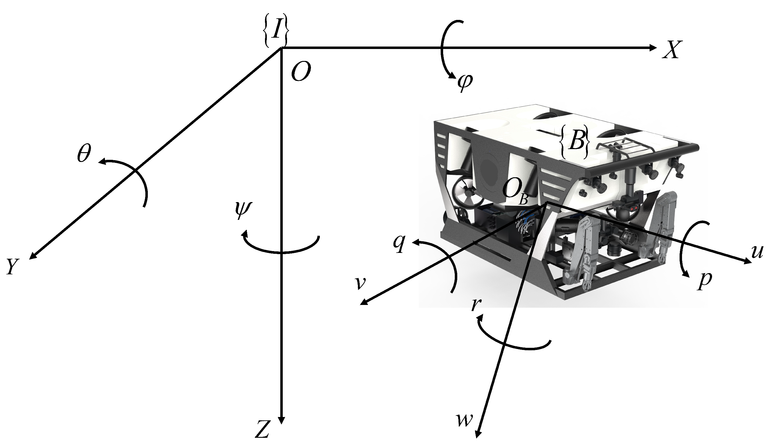
2.3. UUV Kinematics
2.4. UUV Dynamics
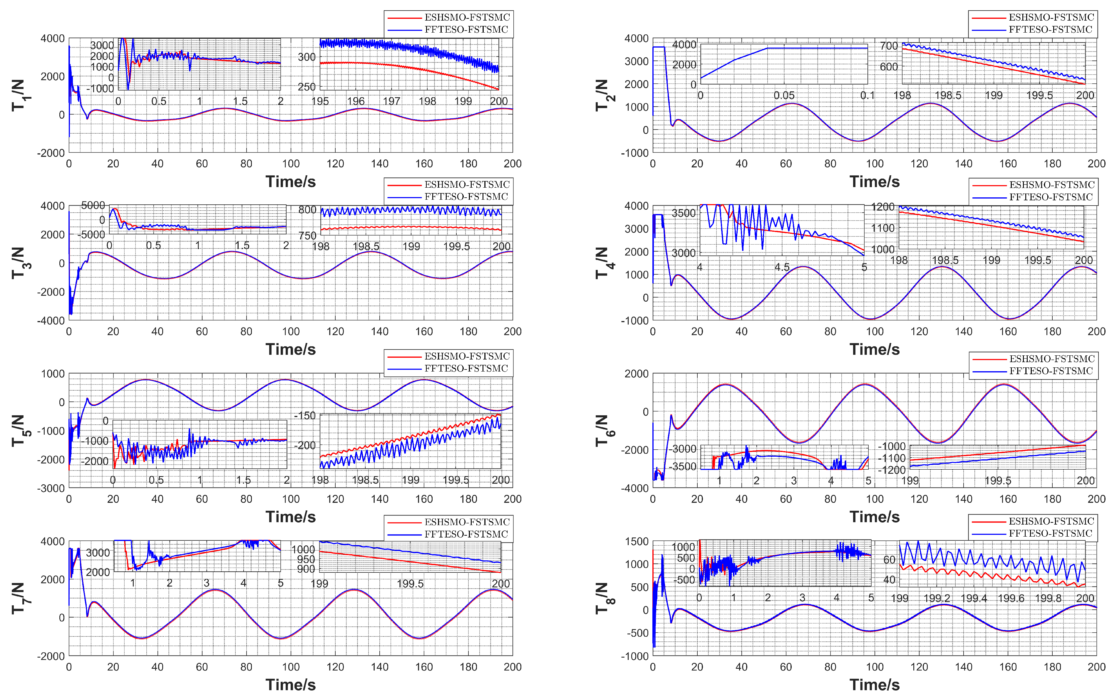
2.5. Thrust Forces Distribution
2.6. Control Objectives
3. Extended State Higher-Order Sliding Mode Observer
3.1. Design of ESHSMO
3.2. Convergence Analysis of ESHSMO
4. Fast Finite-Time Super-Twisting Sliding Mode Control
4.1. Design of FSTSMC
4.2. Stability Analysis of FSTSMC
5. Numerical Simulation and Experimental Verification
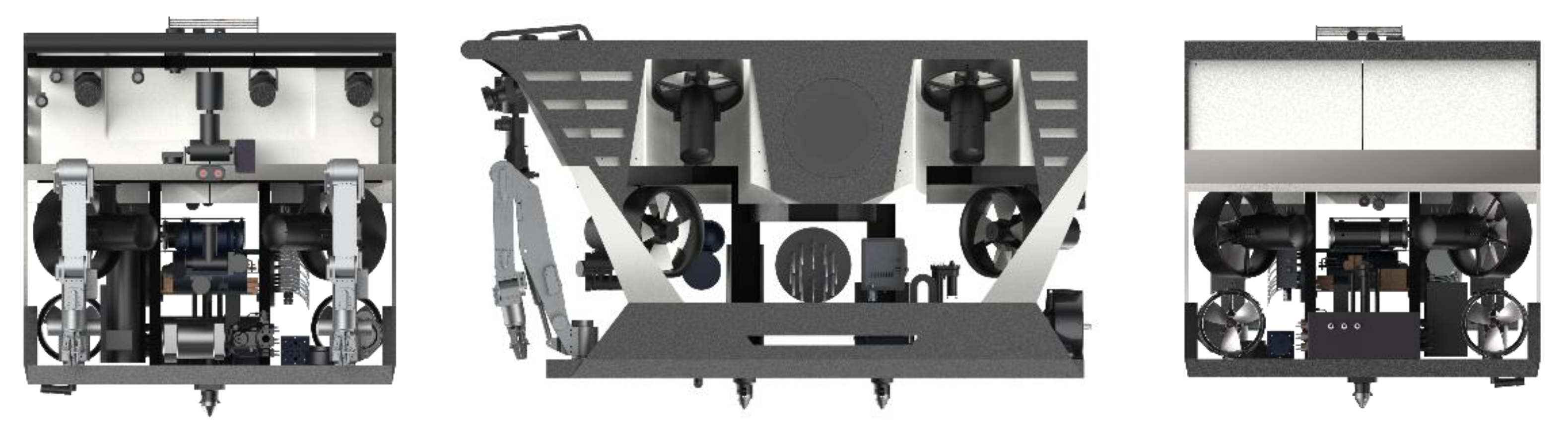
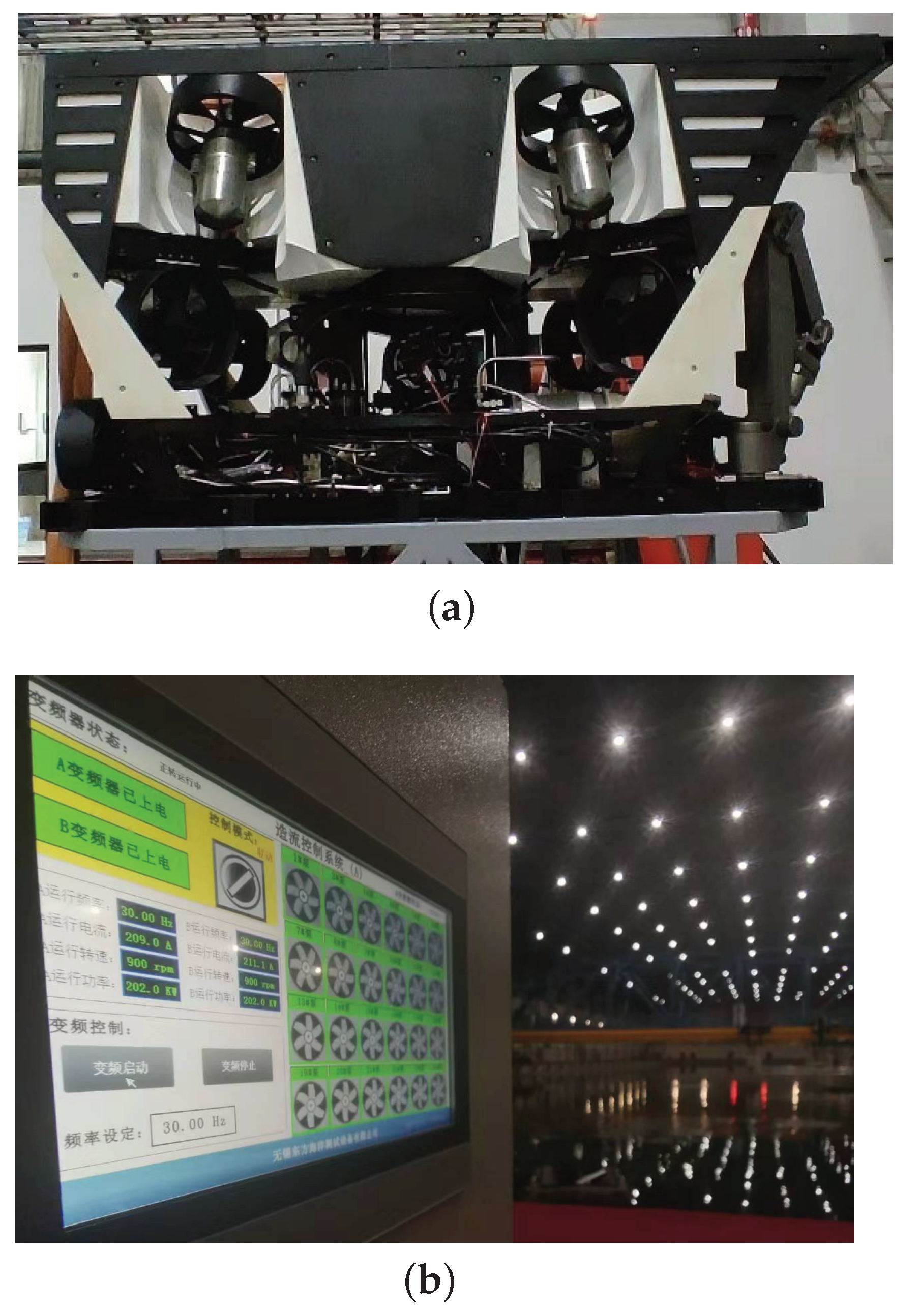
5.1. Uuv Platform
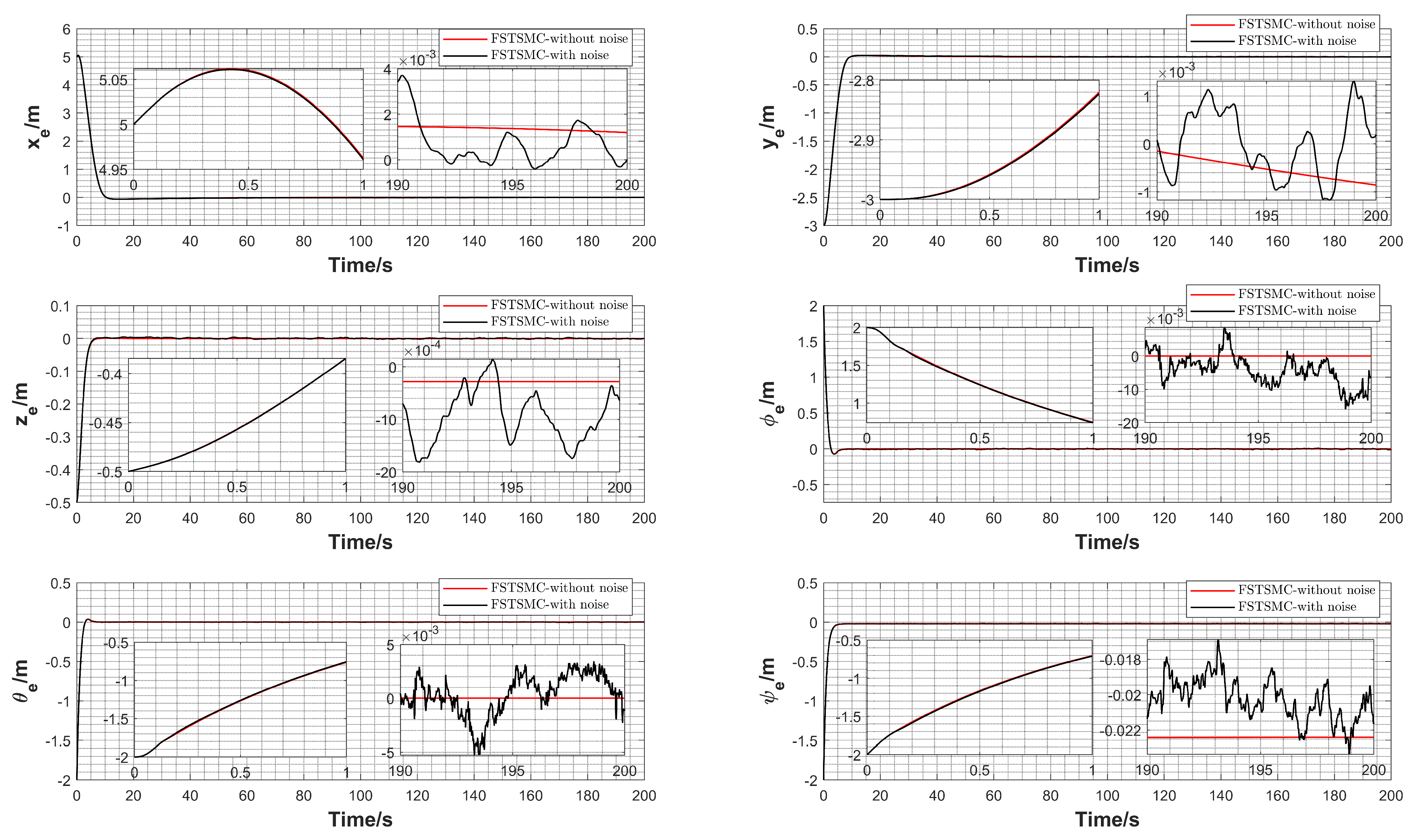
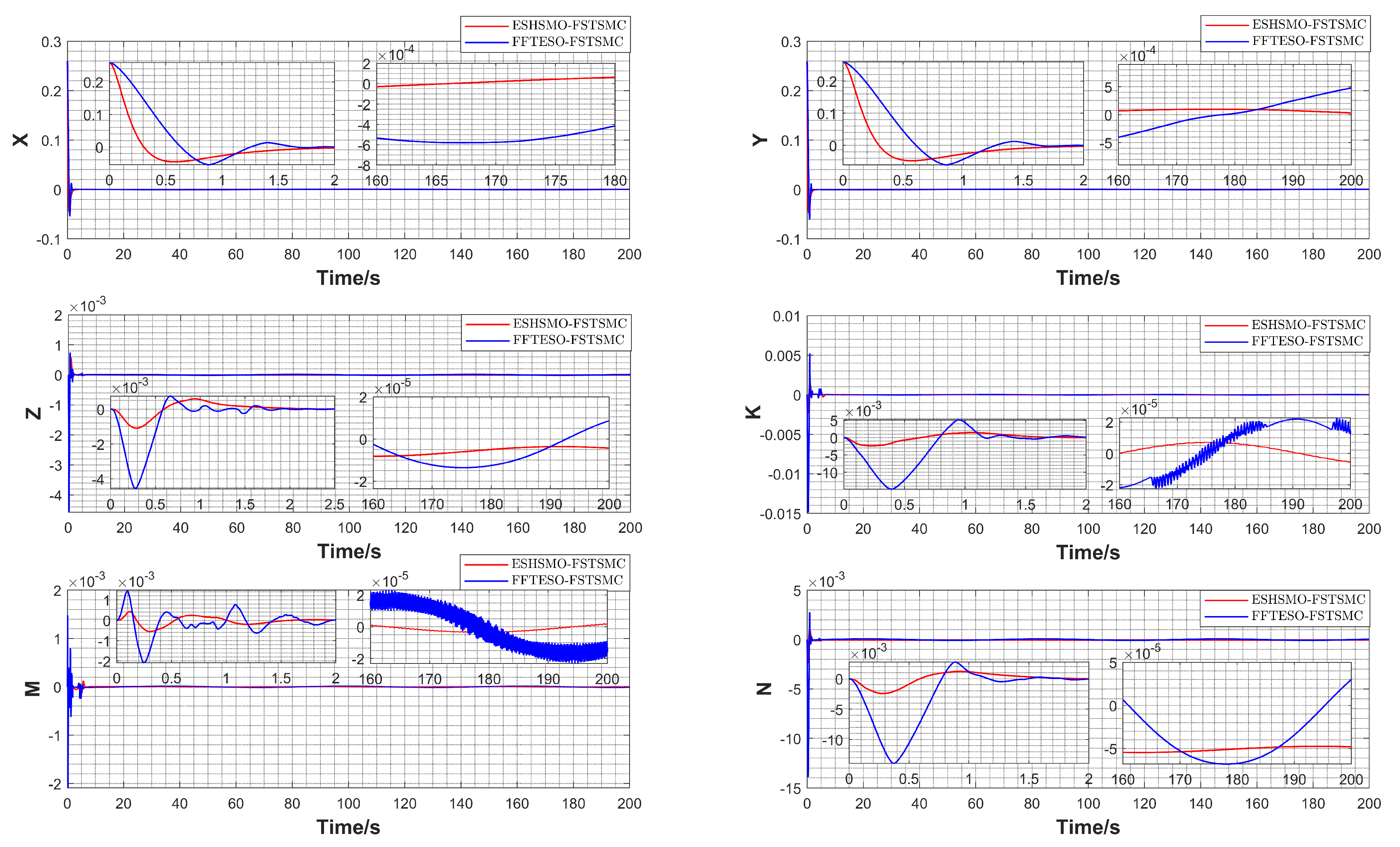
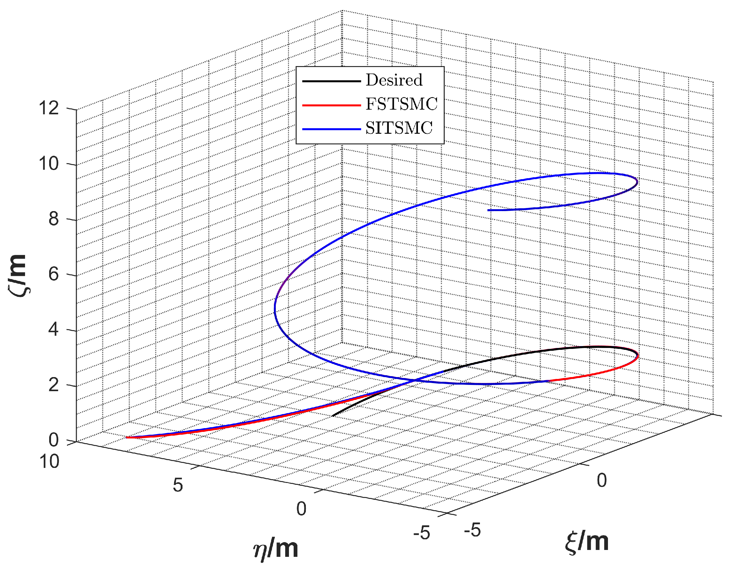
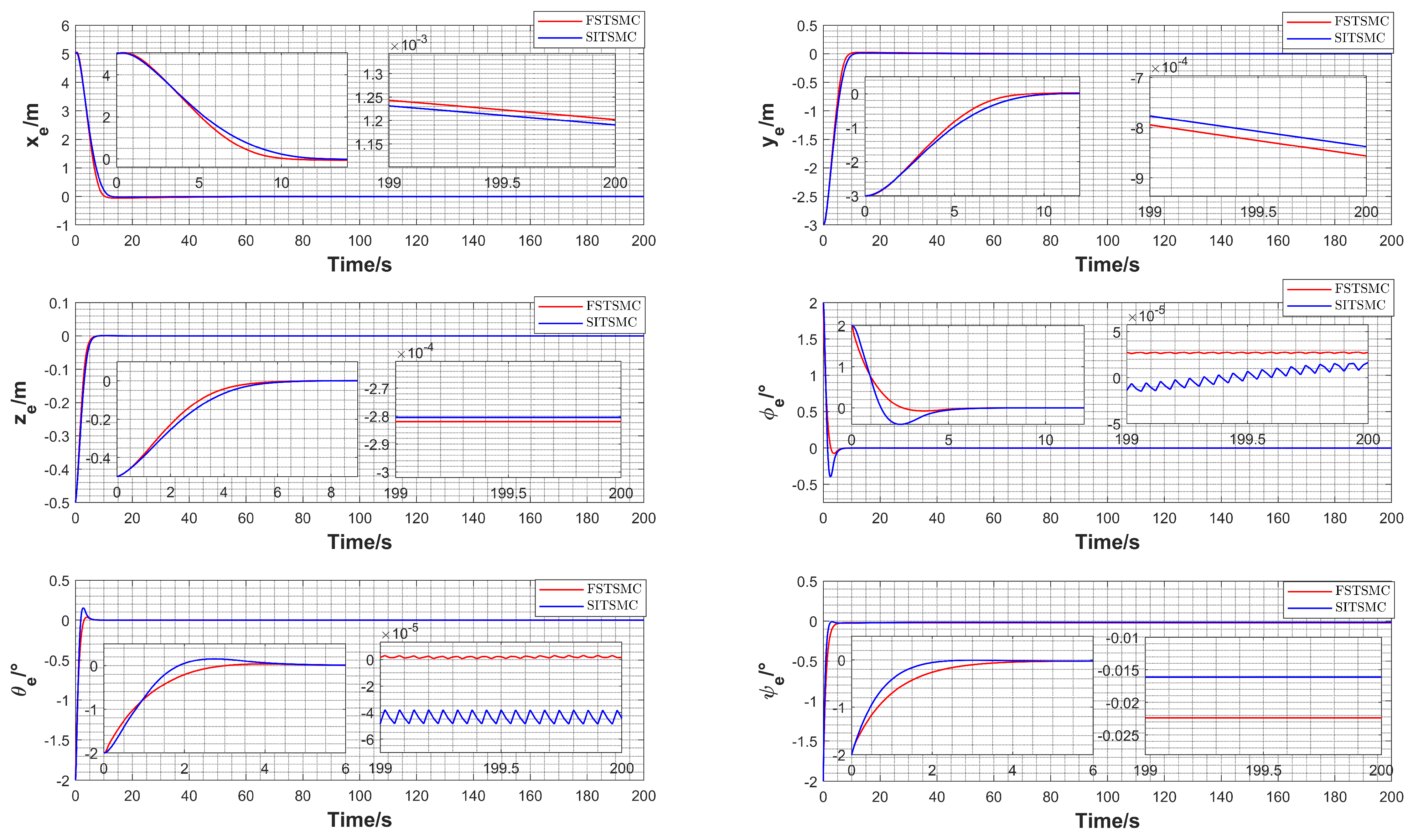
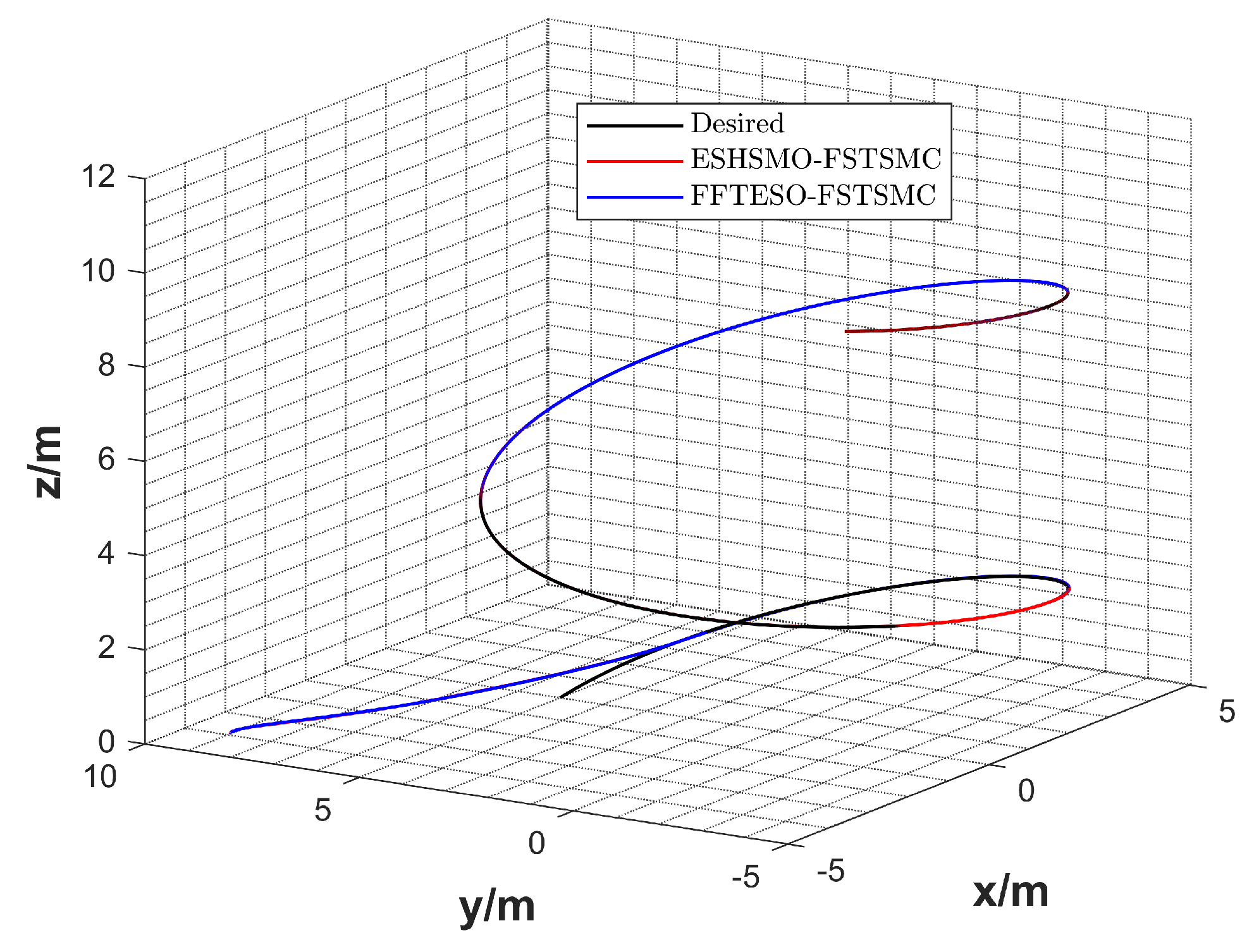
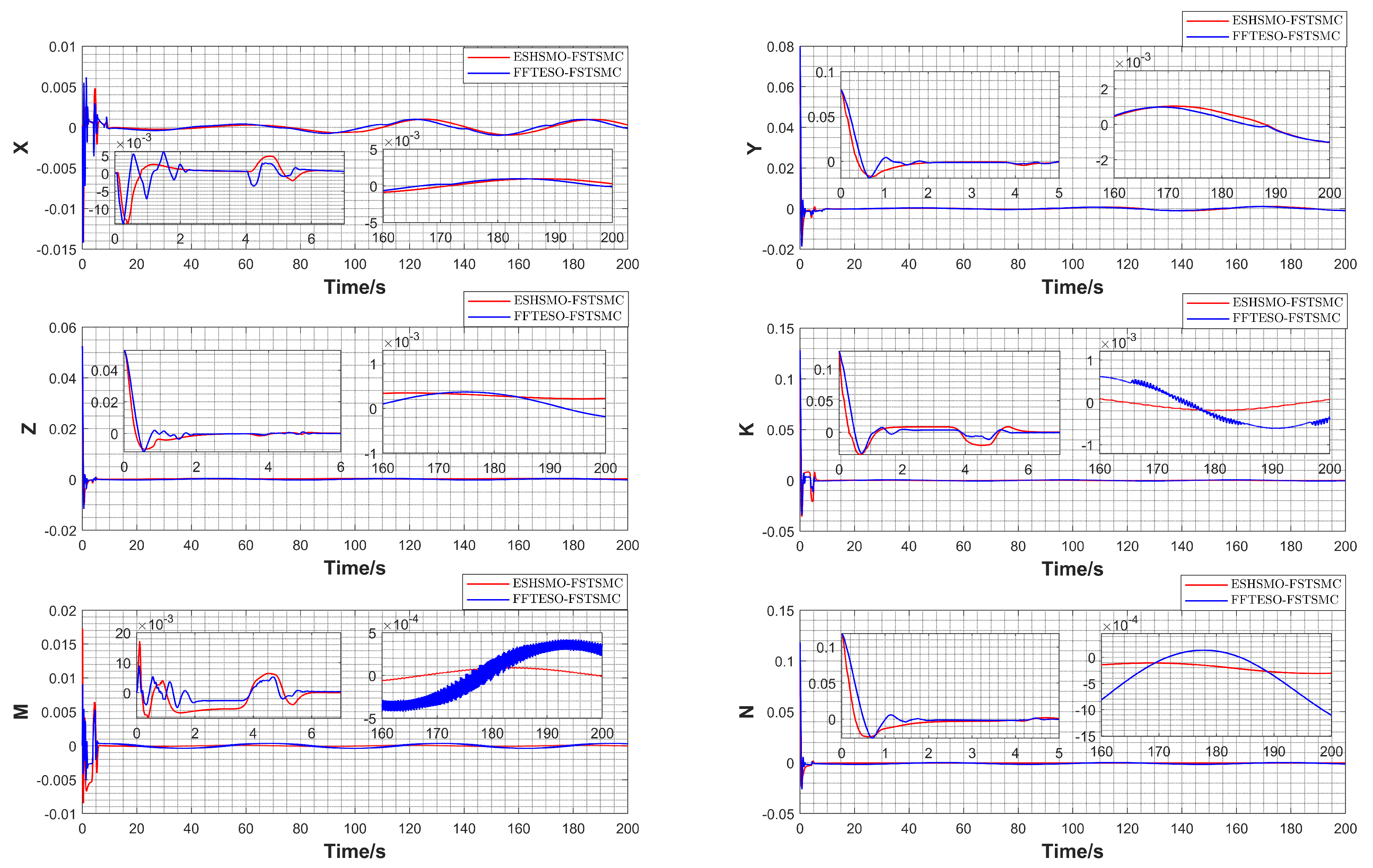
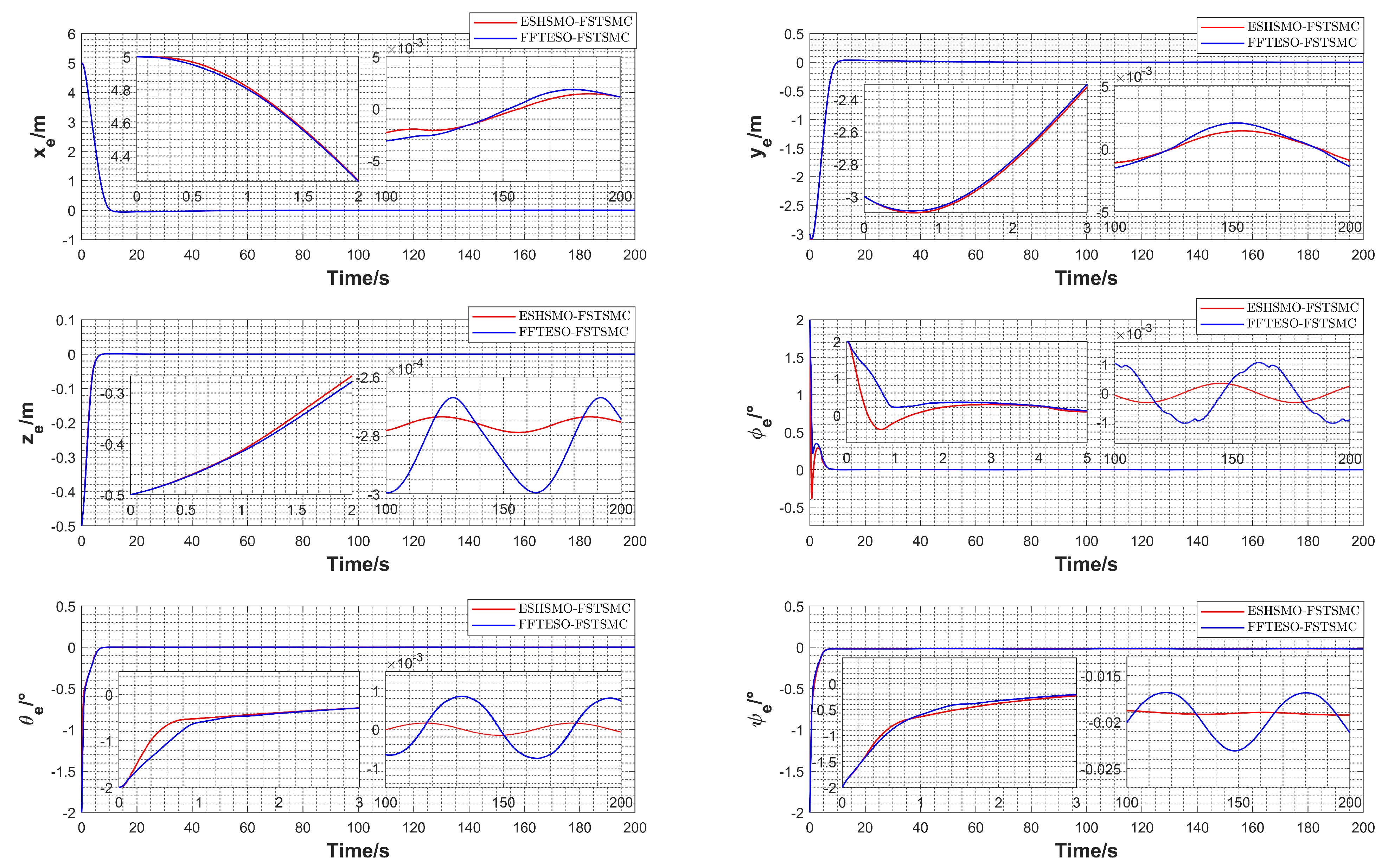
5.2. Numerical Simulation
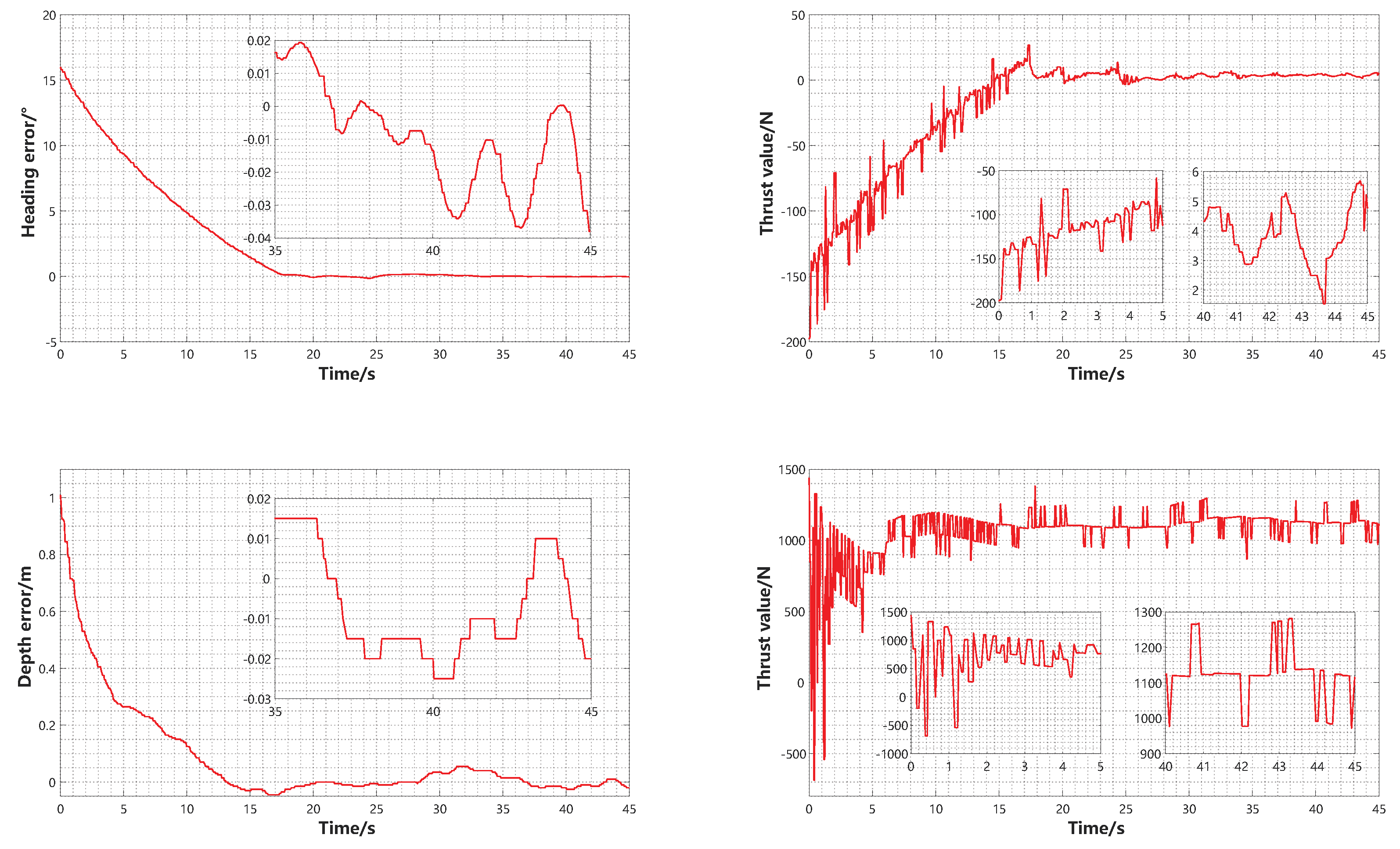
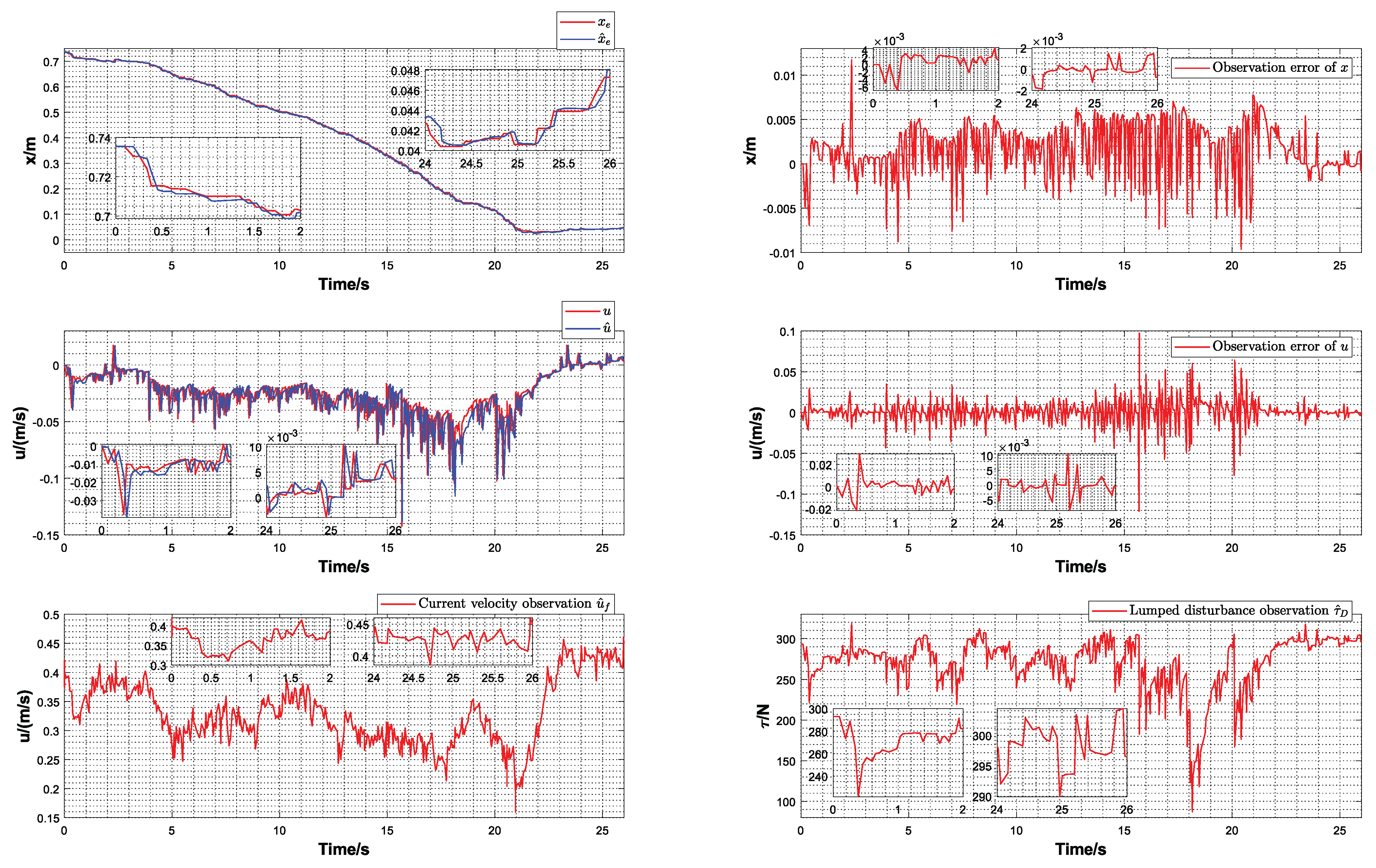
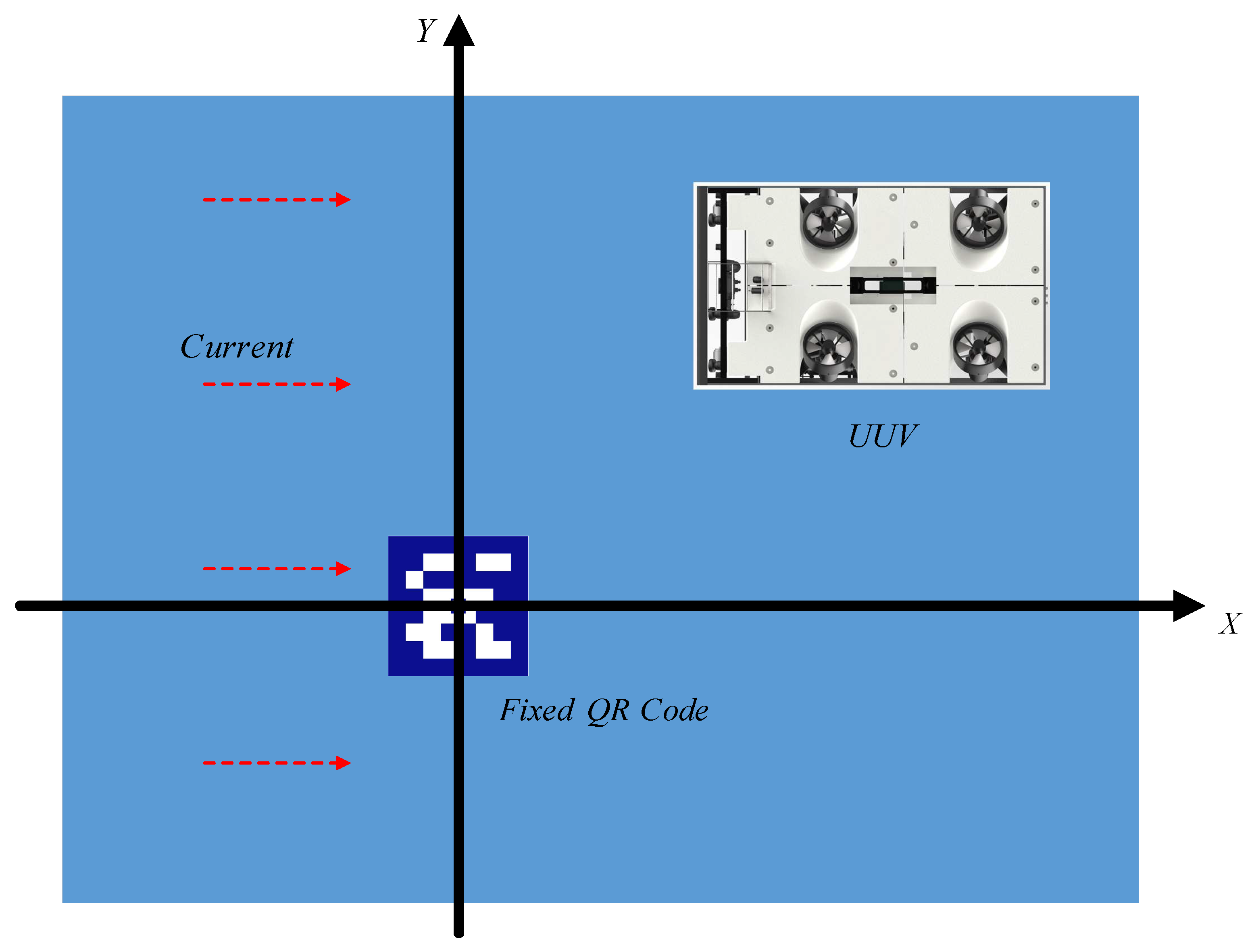
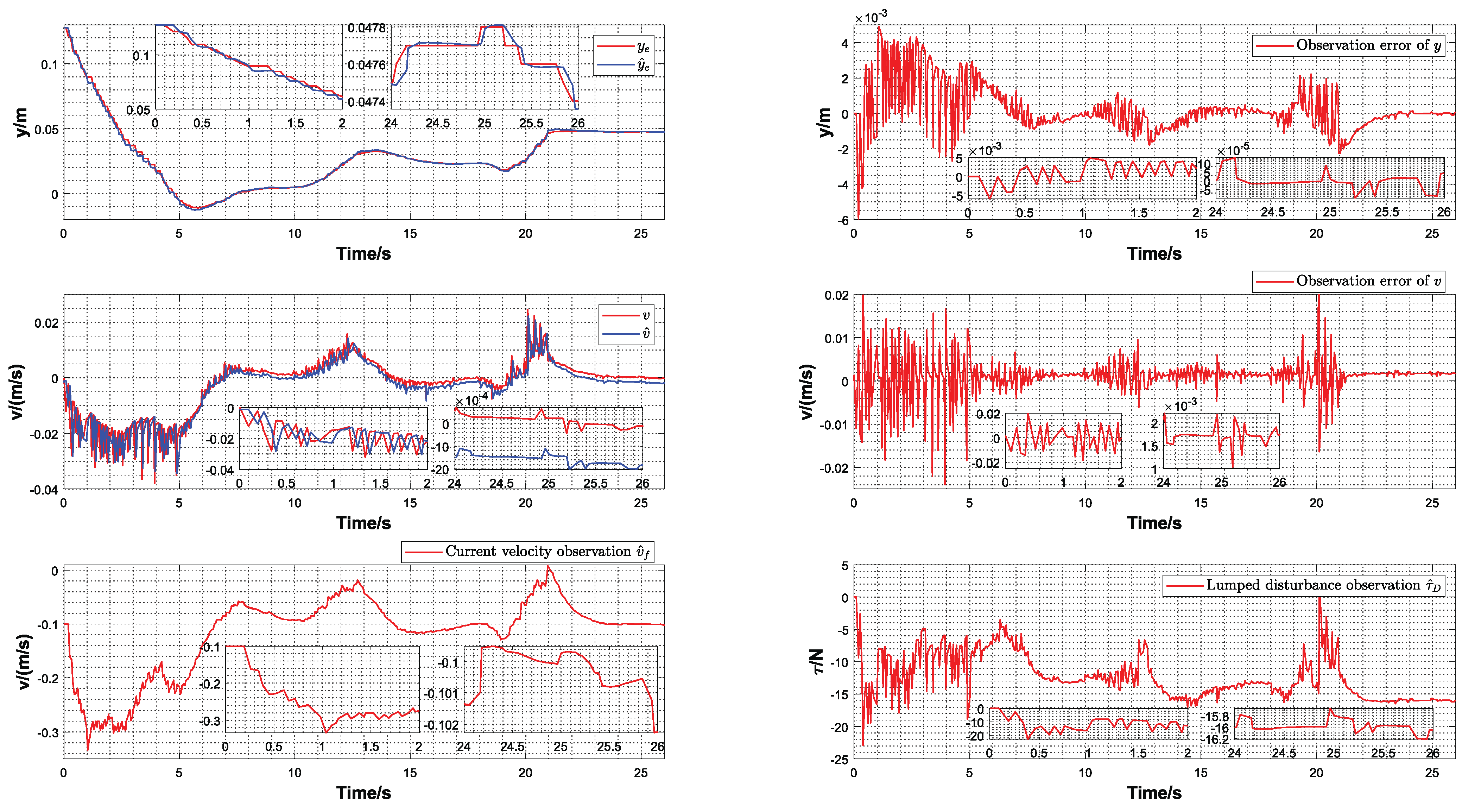
5.3. Experimental Verification
6. Conclusions
Author Contributions
Funding
Institutional Review Board Statement
Informed Consent Statement
Data Availability Statement
Conflicts of Interest
Abbreviations
| FSTSMC | Fast finite-time super-twisting sliding mode control |
| ESHSMO | Extended state higher-order sliding mode observer |
| UUV | Unmanned underwater vehicle |
| PID | Proportion integration differentiation |
| AUV | Autonomous underwater vehicle |
| ESO | Extended state observer |
| STISMC | Super-twisting integral sliding mode control |
| FFTESO | Fast finite-time extended state observer |
References
- Ali, N.; Tawiah, I.; Zhang, W. Finite-time extended state observer based nonsingular fast terminal sliding mode control of autonomous underwater vehicles. Ocean Eng. 2020, 218, 108179. [Google Scholar] [CrossRef]
- Zhang, W.; Wu, W.; Li, Z.; Du, X.; Yan, Z. Three-Dimensional Trajectory Tracking of AUV Based on Nonsingular Terminal Sliding Mode and Active Disturbance Rejection Decoupling Control. J. Mar. Sci. Eng. 2023, 11, 959. [Google Scholar] [CrossRef]
- Lv, T.; Zhou, J.; Wang, Y.; Gong, W.; Zhang, M. Sliding mode based fault tolerant control for autonomous underwater vehicle. Ocean Eng. 2020, 216, 107855. [Google Scholar] [CrossRef]
- Mu, W.; Wang, Y.; Sun, H.; Liu, G. Double-Loop Sliding Mode Controller with An Ocean Current Observer for the Trajectory Tracking of ROV. J. Mar. Sci. Eng. 2021, 9, 1000. [Google Scholar] [CrossRef]
- Elmokadem, T.; Zribi, M.; Youcef-Toumi, K. Terminal sliding mode control for the trajectory tracking of underactuated Autonomous Underwater Vehicles. Ocean Eng. 2017, 129, 613–625. [Google Scholar] [CrossRef]
- Nguyen, X.; Mehdi, G.; Hong, S. Constrained Nonsingular Terminal Sliding Mode Attitude Control for Spacecraft: A Funnel Control Approach. Mathematics 2023, 11, 247. [Google Scholar]
- Nguyen, X.; Mehdi, G. Smooth, Singularity-Free, Finite-Time Tracking Control for Euler–Lagrange Systems. Mathematics 2022, 10, 3850. [Google Scholar]
- Xuan-Mung, N.; Nguyen, N.P.; Pham, D.B.; Dao, N.N.; Nguyen, H.T.; Ha Le Nhu Ngoc, T.; Vu, M.T.; Hong, S.K. Novel gain-tuning for sliding mode control of second-order mechanical systems: Theory and experiments. Sci. Rep. 2023, 13, 10541. [Google Scholar] [CrossRef]
- Wang, W.; Yan, J.; Wang, H.; Ge, H.; Zhu, Z.; Yang, G. Adaptive MPC trajectory tracking for AUV based on Laguerre function. Ocean Eng. 2022, 261, 111870. [Google Scholar] [CrossRef]
- Li, J.; Xia, Y.; Xu, G.; He, Z.; Xu, K.; Xu, G. Three-Dimensional Prescribed Performance Tracking Control of UUV via PMPC and RBFNN-FTTSMC. J. Mar. Sci. Eng. 2023, 11, 1357. [Google Scholar] [CrossRef]
- Li, S.; Xu, C.; Liu, J.; Han, B. Data-driven docking control of autonomous double-ended ferries based on iterative learning model predictive control. Ocean Eng. 2023, 273, 113994. [Google Scholar] [CrossRef]
- Long, C.; Qin, X.; Bian, Y.; Hu, M. Trajectory tracking control of ROVs considering external disturbances and measurement noises using ESKF-based MPC. Ocean Eng. 2021, 241, 109991. [Google Scholar] [CrossRef]
- Zhang, J.; Xiang, X.; Lapierre, L.; Zhang, Q.; Li, W. Approach-angle-based three-dimensional indirect adaptive fuzzy path following of under-actuated AUV with input saturation. Appl. Ocean Res. 2021, 107, 102486. [Google Scholar] [CrossRef]
- Yu, C.; Xiang, X.; Wilson, P.A.; Zhang, Q. Guidance-error-based robust fuzzy adaptive control for bottom following of a flight-style AUV with saturated actuator dynamics. IEEE Trans. Cybern. 2020, 50, 1887–1899. [Google Scholar] [CrossRef] [PubMed]
- Miao, J.; Sun, X.; Chen, Q.; Zhang, H.; Liu, W.; Wang, Y. Robust Path-Following Control for AUV under Multiple Uncertainties and Input Saturation. Drones 2023, 7, 665. [Google Scholar] [CrossRef]
- Che, G. Single critic network based fault-tolerant tracking control for underactuated AUV with actuator fault. Ocean Eng. 2022, 254, 111380. [Google Scholar] [CrossRef]
- Xuan-Mung, N.; Golestani, M.; Hong, S.-K. Tan-Type BLF-Based Attitude Tracking Control Design for Rigid Spacecraft with Arbitrary Disturbances. Mathematics 2022, 10, 4548. [Google Scholar] [CrossRef]
- Wan, J.; Liu, H.; Yuan, J.; Shen, Y.; Zhang, H.; Wang, H.; Zheng, Y. Motion Control of Autonomous Underwater Vehicle Based on Fractional Calculus Active Disturbance Rejection. J. Mar. Sci. Eng. 2021, 9, 1306. [Google Scholar] [CrossRef]
- Lamraoui, H.C.; Qidan, Z. Path following control of fully-actuated autonomous underwater vehicle in presence of fast-varying disturbances. Appl. Ocean Res. 2019, 86, 40–46. [Google Scholar] [CrossRef]
- An, L.; Li, Y.; Cao, J.; Jiang, Y.; He, J.; Wu, H. Proximate time optimal for the heading control of underactuated autonomous underwater vehicle with input nonlinearities. Appl. Ocean Res. 2020, 95, 102002. [Google Scholar] [CrossRef]
- Zhou, Y.; Sun, X.; Sang, H.; Yu, P. Robust dynamic heading tracking control for wave gliders. Ocean Eng. 2022, 256, 111510. [Google Scholar] [CrossRef]
- Liu, J.; Zhao, M.; Qiao, L. Adaptive barrier Lyapunov function-based obstacle avoidance control for an autonomous underwater vehicle with multiple static and moving obstacles. Ocean Eng. 2022, 243, 110303. [Google Scholar] [CrossRef]
- Guo, J.; Wang, J.; Bo, Y. An observer-based adaptive neural network finite-time tracking control for autonomous underwater vehicles via command filters. Drones 2023, 7, 604. [Google Scholar] [CrossRef]
- Zhao, J.; Qin, Y.; Hu, C.; Xu, G.; Xu, K.; Xia, Y. Robust Adaptive Backstepping Motion Control of Underwater Cable-Driven Parallel Mechanism Using Improved Linear Model Predictive Control. J. Mar. Sci. Eng. 2023, 11, 1173. [Google Scholar] [CrossRef]
- Makavita, C.D.; Jayasinghe, S.G.; Nguyen, H.D.; Ranmuthugala, D. Experimental comparison of two composite MRAC methods for UUV operations with low adaptation gains. IEEE J. Ocean. Eng. 2020, 45, 227–246. [Google Scholar] [CrossRef]
- Nguyen, X.; Mehdi, G. Energy-Efficient Disturbance Observer-Based Attitude Tracking Control With Fixed-Time Convergence for Spacecraft. IEEE Trans. Aerosp. Electron. Syst. 2023, 59, 3659–3668. [Google Scholar]
- Golestani, M.; Zhang, W.; Yang, Y.; Xuan-Mung, N. Disturbance observer-based constrained attitude control for flexible spacecraft. IEEE Trans. Aerosp. Electron. Syst. 2022, 59, 963–972. [Google Scholar] [CrossRef]
- Mehdi, G.; Seyed, M.; Saleh, M. Fixed-time control for high-precision attitude stabilization of flexible spacecraft. Eur. J. Control 2021, 57, 222–231. [Google Scholar]
- Huang, B.; Yang, Q. Double-loop sliding mode controller with a novel switching term for the trajectory tracking of work-class ROVs. Ocean Eng. 2019, 178, 80–94. [Google Scholar] [CrossRef]
- Labbadi, M.; Cherkaoui, M. Robust adaptive backstepping fast terminal sliding mode controller for uncertain quadrotor UAV. Aerosp. Sci. Technol. 2019, 93, 105306. [Google Scholar] [CrossRef]
- Elmokadem, T.; Zribi, M.; Youcef-Toumi, K. Trajectory tracking sliding mode control of underactuated AUVs. Nonlinear Dyn. 2016, 84, 1079–1091. [Google Scholar] [CrossRef]
- Levant, A. Higher Order Sliding Modes and Their Application for Controlling Uncertain Processes. Ph.D. Dissertation, Institute for System Studies of the USSR Academy of Science, Moscow, Russia, 1987. [Google Scholar]
- Borlaug, I.G.; Pettersen, K.Y.; Gravdahl, J.T. Comparison of two second-order sliding mode control algorithms for an articulated intervention AUV: Theory and experimental results. Ocean Eng. 2021, 222, 108480. [Google Scholar] [CrossRef]
- Manzanilla, A.; Ibarra, E.; Salazar, S. Super-twisting integral sliding mode control for trajectory tracking of an Unmanned Underwater Vehicle. Ocean Eng. 2021, 234, 109164. [Google Scholar] [CrossRef]
- González-García, J.; Gómez-Espinosa, A.; García-Valdovinos, L.G.; Salgado-Jiménez, T.; Cuan-Urquizo, E.; Escobedo Cabello, J.A. Experimental Validation of a Model-Free High-Order Sliding Mode Controller with Finite-Time Convergence for Trajectory Tracking of Autonomous Underwater Vehicles. Sensors 2022, 22, 488. [Google Scholar] [CrossRef] [PubMed]
- Li, X.; Ren, C.; Ma, S.; Zhu, X. Compensated model-free adaptive tracking control scheme for autonomous underwater vehicles via extended state observer. Ocean Eng. 2020, 217, 107976. [Google Scholar] [CrossRef]
- Wu, C.; Dai, Y.; Shan, L.; Zhu, Z.; Wu, Z. Data-driven trajectory tracking control for autonomous underwater vehicle based on iterative extended state observer. Math. Biosci. Eng. MBE 2022, 19, 3036–3055. [Google Scholar] [CrossRef] [PubMed]
- Kim, H.-H.; Lee, M.C.; Cho, H.-J.; Hwang, J.-H.; Won, J.-S. SMCSPO-Based Robust Control of AUV in Underwater Environments including Disturbances. Appl. Sci. 2021, 11, 10978. [Google Scholar] [CrossRef]
- Hu, Q.; Jiang, B. Continuous Finite-Time Attitude Control for Rigid Spacecraft Based on Angular Velocity Observer. IEEE Trans. Aerosp. Electron. Syst. 2018, 54, 1082–1092. [Google Scholar] [CrossRef]
- Li, S.; Du, H.; Lin, X. Finite-time consensus algorithm for multi-agent systems with double-integrator dynamics. Automatica 2011, 47, 1706–1712. [Google Scholar] [CrossRef]
- Fossen, T.I. Marine Control Systems. Marine Cybernetics. 2002. Available online: http://kashti.ir/files/ENBOOKS/Marine%20control%20systems.pdf (accessed on 23 January 2024).
- Abdurahman, B.; Savvaris, A.; Tsourdos, A. Switching LOS guidance with speed allocation and vertical course control for path-following of unmanned underwater vehicles under ocean current disturbances. Ocean Eng. 2019, 182, 412–426. [Google Scholar] [CrossRef]


| Serial Number of the Thrusters | Description | x | y | z | Angle of Installation | |
|---|---|---|---|---|---|---|
| Horizontal thrusters | 1 | Bow left horizontal thruster | 1.250 | −0.960 | −0.185 | 35° to axis |
| 2 | Bow right horizontal thruster | 1.250 | 0.960 | −0.185 | −35° to axis | |
| 3 | Stern left horizontal thruster | −1.250 | −0.960 | −0.185 | 145° to axis | |
| 4 | Stern right horizontal thruster | −1.250 | 0.960 | −0.185 | 215° to axis | |
| Vertical thrusters | 5 | Bow left vertical thruster | 0.925 | −0.678 | −0.875 | 10° to axis |
| 6 | Bow right vertical thruster | 0.925 | 0.678 | −0.875 | −10° to axis | |
| 7 | Stern left vertical thruster | −0.925 | -0.678 | −0.875 | 10° to axis | |
| 8 | Stern right vertical thruster | −0.925 | 0.678 | −0.875 | −10° to axis | |
| Performance Indicators | Control Approach | x | y | z | |||
|---|---|---|---|---|---|---|---|
| Root mean square error | FSTSMC | 0.6570 | 0.3468 | 0.0411 | 0.1013 | 0.1034 | 0.1001 |
| STISMC | 0.6633 | 0.3542 | 0.0429 | 0.1143 | 0.1082 | 0.0840 | |
| Convergence time | FSTSMC | 8.54 | 7.36 | 4.52 | 2.20 | 2.38 | 3.06 |
| STISMC | 9.86 | 8.34 | 5.00 | 4.36 | 3.54 | 1.74 | |
| Steady-state error | FSTSMC | 0.0012 | −0.00084 | −0.00028 | 2.7 × | 1.6 × | −0.022 |
| STISMC | 0.0012 | -0.00086 | −0.00028 | 1.7 × | −4.5 × | −0.016 |
| Performance Indicators | Control Scheme | x | y | z | |||
|---|---|---|---|---|---|---|---|
| Root mean square error of lumped disturbance observation | ESHSMO-FSTSMC | 0.0066 | 0.0066 | 4.6 × | 1.1 × | 2.3 × | 1.2 × |
| FFTESO-FSTSMC | 0.0094 | 0.0093 | 1.5 × | 6.0 × | 6.2 × | 5.3 × | |
| Root mean square error of ocean current velocity observation | ESHSMO-FSTSMC | 7.9 × | 0.0023 | 0.0014 | 0.0035 | 8.9 × | 0.0031 |
| FFTESO-FSTSMC | 7.4 × | 0.0026 | 0.0016 | 0.0042 | 5.4 × | 0.0039 | |
| Root mean square error of trajectory tracking | ESHSMO-FSTSMC | 0.6417 | 0.4050 | 0.0440 | 0.0686 | 0.0926 | 0.0984 |
| FFTESO-FSTSMC | 0.6427 | 0.4075 | 0.0447 | 0.0958 | 0.1047 | 0.0975 | |
| Convergence time | ESHSMO-FSTSMC | 8.76 | 8.22 | 5.34 | 4.78 | 4.82 | 4.32 |
| FFTESO-FSTSMC | 8.78 | 8.26 | 5.40 | 5.18 | 5.00 | 4.36 | |
| Steady-state error | ESHSMO-FSTSMC | 0.00112 | −0.00091 | −0.00027 | 0.00024 | −7.2 × | −0.019 |
| FFTESO-FSTSMC | 0.00112 | −0.00141 | −0.00027 | −0.00092 | 0.00073 | −0.021 |
Disclaimer/Publisher’s Note: The statements, opinions and data contained in all publications are solely those of the individual author(s) and contributor(s) and not of MDPI and/or the editor(s). MDPI and/or the editor(s) disclaim responsibility for any injury to people or property resulting from any ideas, methods, instructions or products referred to in the content. |
© 2024 by the authors. Licensee MDPI, Basel, Switzerland. This article is an open access article distributed under the terms and conditions of the Creative Commons Attribution (CC BY) license (https://creativecommons.org/licenses/by/4.0/).
Share and Cite
Guo, L.; Liu, W.; Li, L.; Xu, J.; Zhang, K.; Zhang, Y. Fast Finite-Time Super-Twisting Sliding Mode Control with an Extended State Higher-Order Sliding Mode Observer for UUV Trajectory Tracking. Drones 2024, 8, 41. https://doi.org/10.3390/drones8020041
Guo L, Liu W, Li L, Xu J, Zhang K, Zhang Y. Fast Finite-Time Super-Twisting Sliding Mode Control with an Extended State Higher-Order Sliding Mode Observer for UUV Trajectory Tracking. Drones. 2024; 8(2):41. https://doi.org/10.3390/drones8020041
Chicago/Turabian StyleGuo, Liwei, Weidong Liu, Le Li, Jingming Xu, Kang Zhang, and Yuang Zhang. 2024. "Fast Finite-Time Super-Twisting Sliding Mode Control with an Extended State Higher-Order Sliding Mode Observer for UUV Trajectory Tracking" Drones 8, no. 2: 41. https://doi.org/10.3390/drones8020041
APA StyleGuo, L., Liu, W., Li, L., Xu, J., Zhang, K., & Zhang, Y. (2024). Fast Finite-Time Super-Twisting Sliding Mode Control with an Extended State Higher-Order Sliding Mode Observer for UUV Trajectory Tracking. Drones, 8(2), 41. https://doi.org/10.3390/drones8020041