Abstract
Drones are an increasingly popular choice for wildlife surveys due to their versatility, quick response capabilities, and ability to access remote areas while covering large regions. A novel application presented here is to combine drone imagery with neural networks to assess mortality within a bird colony. Since 2021, Highly Pathogenic Avian Influenza (HPAI) has caused significant bird mortality in the UK, mainly affecting aquatic bird species. The world’s largest northern gannet colony on Scotland’s Bass Rock experienced substantial losses in 2022 due to the outbreak. To assess the impact, RGB imagery of Bass Rock was acquired in both 2022 and 2023 by deploying a drone over the island for the first time. A deep learning neural network was subsequently applied to the data to automatically detect and count live and dead gannets, providing population estimates for both years. The model was trained on the 2022 dataset and achieved a mean average precision (mAP) of 37%. Application of the model predicted 18,220 live and 3761 dead gannets for 2022, consistent with NatureScot’s manual count of 21,277 live and 5035 dead gannets. For 2023, the model predicted 48,455 live and 43 dead gannets, and the manual count carried out by the Scottish Seabird Centre and UK Centre for Ecology and Hydrology (UKCEH) of the same area gave 51,428 live and 23 dead gannets. This marks a promising start to the colony’s recovery with a population increase of 166% determined by the model. The results presented here are the first known application of deep learning to detect dead birds from drone imagery, showcasing the methodology’s swift and adaptable nature to not only provide ongoing monitoring of seabird colonies and other wildlife species but also to conduct mortality assessments. As such, it could prove to be a valuable tool for conservation purposes.
1. Introduction
Drones, also known as Unmanned Aerial Vehicles (UAVs), are increasingly popular for wildlife conservation due to their versatility, quick response capabilities, and ability to access remote areas while covering large regions. Seabirds, nesting in vast and hard-to-reach colonies, benefit greatly from drones, as they avoid disturbances caused by ground surveys []. Their diverse applications include estimating deer populations [], monitoring whale health [], and detecting the tracks of nesting turtles []. Technological advancements have resulted in higher-resolution imagery and video, more sensitive detectors, longer battery life, and quieter motors, crucial for approaching wildlife without causing disturbance. The drones’ hovering capability also ensures clearer images by eliminating motion blur from camera movement.
Since November 2021, a record number of cases of Highly Pathogenic Avian Influenza H5N1 (HPAI) have been confirmed in the UK []. HPAI spreads through saliva, nasal secretions, or droppings and has caused tens of thousands of bird deaths across 65 different species, with a particular impact on aquatic bird populations []. One colony that suffered a huge loss in its wake is that of the northern gannet, located on Scotland’s Bass Rock.
Scotland is home to 58% of the world’s northern gannets, Morus bassanus. Northern gannets are large, colonially breeding seabirds. Their striking white and black plumage, densely packed colonies, and long breeding season (March–October) make them a conspicuous feature of coastal systems. The largest individual colony can be found on Bass Rock, located in the Firth of Forth off the East Lothian coastline ([]; Figure 1). At the seasonal peak, over 150,000 gannets can be found on Bass Rock, making it a Site of Specific Scientific Interest (SSSI; []).
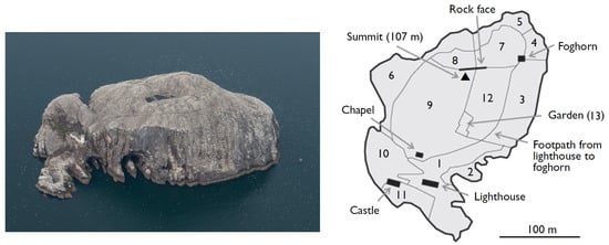
Figure 1.
Left: Aerial view of the study site—Bass Rock (N 566′, W 236′). Image credit: UK Centre for Ecology and Hydrology. Right: Delimited areas used for counting during the previous decadal censuses. Image taken from Murray et al. (2014) [].
Unfortunately, HPAI was detected on Bass Rock in mid-June 2022 and had a devastating effect on the northern gannet colony, resulting in both high adult mortality and breeding failure. With HPAI now moving through seabird populations for the third year in a row as of the end of 2023 [], carrying out regular survey work will be of great importance. These surveys will play a crucial role in monitoring disease progression and assessing the recovery of decimated seabird colonies by conducting population counts. The advent of drone technology promises to make a particular impact on how and when these surveys are conducted, offering a quick and flexible solution.
1.1. Population Census
Gannets are relatively straightforward to count compared to many other species of seabird due to their large size and regular nesting dispersion. The recommended time for counting is June/July, during the middle of the breeding season. Approximately decadal surveys of Bass Rock have been carried out since the mid-1990s using a small fixed-wing plane and observer (or observers) taking aerial photos using film/digital cameras []. Results from these surveys have documented a sustained increase in population size as indicated by the number of Apparently Occupied Sites (AOSs), defined as sites occupied by one or two gannets irrespective of whether nest material is present ([]; Table 1). However, the methodology faces limitations in its logistics, including the need for a suitable aircraft with an experienced pilot and a team of photographers on standby for good conditions. It was also noted in Murray et al. [] that the lack of standardisation in counting units used between colonies across Scotland makes it difficult to produce an accurate total. The final number typically involves combining the total AOSs from most colonies, with counts of individual nests at others.

Table 1.
Counts of Apparently Occupied Sites (AOSs) for northern gannets on Bass Rock as published by previous surveys: 2014, 2009 [], 2004, 1994, and 1985 [].
Previous aerial surveys of the Bass Rock gannetry have required the manual counting of AOSs on discrete images by at least two experienced individuals. The method involved sub-dividing Bass Rock into distinct count sections based on the topography of the cliffs (Figure 1) and marking off the AOSs as they are noted using basic photo editing software. Obvious groups of birds with immature plumage that are clearly not breeding were not counted. Even when counters are highly experienced and motivated, this method is time-consuming and the criteria for identifying AOSs are subjective. Comparisons of independent counts by different individuals highlight the potential for inter-observer variation, which tends to be greater when the resolution of the images is poorer. More generally, manual counts tend to become more prone to human error as the dataset and colony size increase due to, e.g., tiredness, boredom of repetition, or distraction [,,]. Thus, carrying out a complete, replicated manual count of a large seabird colony can take days, or even weeks.
1.2. Drones and Deep Learning as the Solution
The combination of Bass Rock’s location and the unpredictable Scottish weather makes drones a cost-effective, convenient, and efficient means of acquiring imagery compared to fixed-wing plane surveys. As such, the HPAI outbreak provided an opportune time to evaluate how drones could be used to provide a swifter and more standardised method for assessing the population of northern gannets on Bass Rock.
For counting individuals, the logical replacement to performing it manually is to use Artificial Neural Networks (ANNs) capable of supervised learning to automatically detect gannets in an image. This increases counting speed and accuracy. ANNs consist of ‘node layers’, where individual nodes acts like artificial neurons connecting to the next. Each node has an associated weight, representing the importance of features in predicting the presence of an object, and a threshold value, above which the node is ‘activated’ and data are passed to the next layer for further learning. A ‘deep’ neural network consists of at least four layers: an input layer, two or more hidden layers, and an output layer []. This approach is commonly known as Deep Learning (DL).
Publications applying DL techniques to wildlife observations have only really appeared in the past 5–7 years, mostly in response to the technology becoming easier to use by non-technical specialists []. Since 2019, a growing number of studies have been published showcasing how drone imagery and DL can be effectively used for bird population-related research. These studies include estimating breeding numbers of West African terns [], detecting changes in Turkish migrating bird populations [], and monitoring black-browed albatrosses and southern rockhopper penguins on the Falkland Islands []. A paper by Hong et al. [] also focuses on comparing DL architectures for the detection of different bird species in drone imagery.
Currently, only a few publications have utilised machine learning techniques to analyse images of gannets specifically. Dujon et al. [] conducted a proof-of-concept study using a Convolutional Neural Network (CNN) on drone imagery of Australian gannets (Morus serrator) to develop an algorithm capable of monitoring multiple species. More recently, Kuru et al. [] developed a platform to improve detection accuracy in offshore marine wildlife surveys, training their system using images of northern gannets captured from a manned aircraft.
There is a notable absence in the literature regarding the development of a deep learning model that can distinguish between living and dead birds. Only one publication was found that explored the use of machine learning for detecting dead birds, focusing on observing commercial poultry in a barn using night-vision cameras []. Furthermore, no known publication has utilised deep learning specifically for monitoring bird colonies after an HPAI outbreak. This knowledge gap highlights two critical areas that this study aims to address: (a) using neural networks to detect and count dead birds within a colony from drone imagery and (b) applying this methodology to assess the impact of HPAI by comparing counts of individual birds from 2022 and 2023.
2. Materials and Methods
Figure 2 shows an example workflow for developing the deep learning model, and Figure 3 shows the overall workflow for the project.
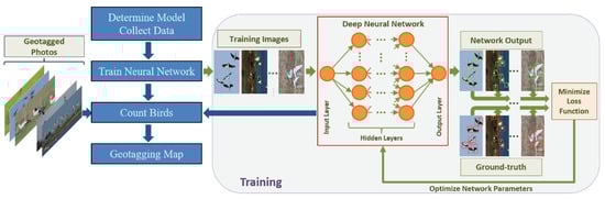
Figure 2.
Basic workflow for a standard DL Convolutional Neural Network (CNN) training process. Image taken from Akçay et al. [].
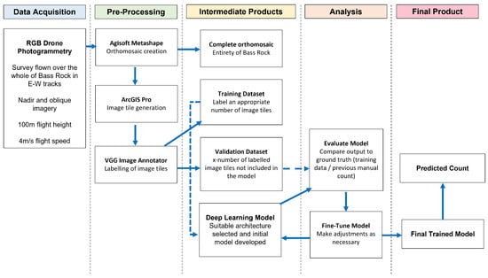
Figure 3.
Complete workflow for the research project, from data acquisition to final product.
2.1. Surveys and Data Preparation
The University of Edinburgh in collaboration with the Scottish Seabird Centre conducted a photogrammetry survey of Bass Rock on 30 June 2022—at the peak of the HPAI outbreak—and during the following breeding season on 27 June 2023 using a DJI Matrice 300 RTK drone. The flight parameters for both missions are shown in Table 2, and the camera properties in Table 3.
Table 2.
DJI Matrice 300 RTK flight parameters for the 2022 and 2023 photogrammetry surveys of Bass Rock.
Table 3.
Properties for the Zenmuse L1 and P1 cameras.
The metric of AOS was not used in this study, rather it aimed to seek out and count individual gannets due to ecological considerations beyond the scope of this project’s aims. Distinguishing between individual gannets requires good image resolution. In 2023, the P1 camera with a higher resolution of 45 MP (compared to 20 MP of L1 used in 2022; Table 3) significantly improved the ground sampling distance (GSD) to 1.36 cm (compared to 3.22 cm for 2022 data). This led to a substantial enhancement in overall image quality. To further improve the contrast of gannets against the rock, the exposure compensation for the 2023 flight was slightly lowered to −0.7, aiming to reduce the saturation of white areas of the gannets.
Balancing the need to separate individual birds in the imagery without disturbing the colony involves a trade-off, with priority given to the welfare of the colony. Previous studies have looked at the response of colonial birds in response to drone flights [,,], with the general result being that the careful selection of flight height both minimised disturbance and prevented habituation to its presence. Any birds that did move in response to the drone quickly regained composure with no ill-effect.
Many of the best practices presented in Edney et al. (2023) [] were adopted to help minimise the disturbance to the gannet colony, with on-site advice and guidance provided by ecologists from the Scottish Seabird Centre during each trip to Bass Rock. For example, the drone take-off/landing site was a marked helipad on the southern tip of the island, away from the main breeding areas, and in such a location that the flight height and parameters could be adjusted out at sea away from the majority of the colony before being brought back in for the survey flight. During the 2022 survey, it was determined that a flight altitude of around 100 m above the surface worked well, with minimal disturbance to the gannets both on the ground and in the air. If a gannet did approach while in the air, usually while close to the water’s edge as they were coming in/out for feeding, all drone movement would be immediately halted and the birds would swoop out of the way. Once the path was clear again, the drone flight was continued.
The standard line-of-sight rules for drone flights were employed, which did mean that some of the surface and cliff faces to the far north of the island could not be covered by the surveys presented here. The 2022 data acquisition involved three individual ‘missions’ oriented E–W and stepped up to effectively contour up the slope of the island. Terrain following was not employed, resulting in each mission flying at slightly different fixed heights above the take-off point. In contrast, for the 2023 survey, a flight height of 105 m was used with automated terrain following based on OS 5 m DTM data. This was flown in a single mission oriented S–N, with some additional hand-flown oblique shots from the south end of the island. In both datasets, coordinates were measured using an RTK method, and no ground control points were utilised.
An orthomosaic for both the 2022 and 2023 datasets was generated by passing geo-referenced RGB oblique and nadir drone imagery into Agisoft Metashape []). There were 176 images in total for the 2022 dataset (102 nadir and 76 oblique) and 150 images for the 2023 dataset (135 nadir, 22 oblique). These orthomosaics were then divided into smaller image tiles for training and validating the deep learning model before its application to the complete dataset (Figure 4 and Figure 5).
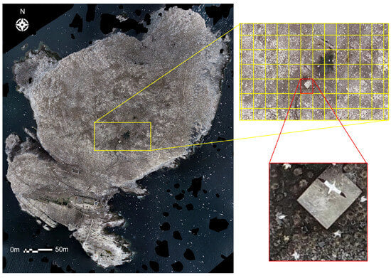
Figure 4.
Example of the tiling process with the 2022 dataset. The entire orthomosaic is split into individual tiles measuring 200 × 200 pixels using the ArcGIS ‘Split Raster’ function. Each 200 × 200 pixel tile (highlighted in red here) equates to 6.4 m on the ground.
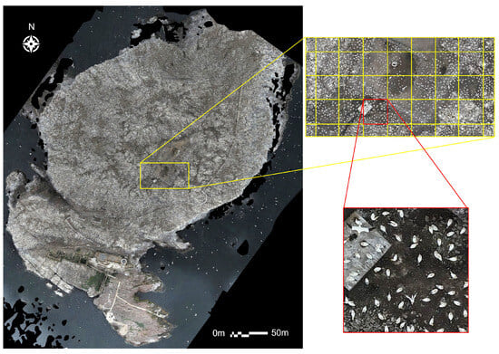
Figure 5.
Example of the tiling process with the 2023 dataset. The entire orthomosaic is split into individual tiles measuring 500 × 500 pixels using the ArcGIS ‘Split Raster’ function. Each 500 × 500 tile (highlighted in red here) equates to 6.8 m on the ground.
The division was accomplished using ArcGIS Pro’s ‘Split Raster’ function within the Image Analyst toolbox [], with a tile size of 200 × 200 pixels for the 2022 dataset, chosen to make the birds appear large enough for labelling without appearing too ‘fuzzy’ (Figure 6, Top Left). Due to the higher resolution of the camera used to acquire the dataset, the gannets appeared much larger in terms of pixel size on the 2023 imagery when split into 200 × 200 pixel tiles, compared to the 2022 imagery (Figure 6, Top Right). This resulted in an issue when attempting to run the model on the 2023 data, as it failed to recognise the gannets for what they were. Therefore, the tile size was varied through trial and error until the relative size of the gannet on the tile roughly matched that of the 2022 tiles, which turned out to be around 500 × 500 pixels (Figure 6, Bottom right).
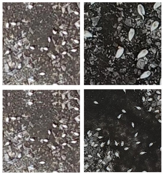
Figure 6.
Top Left and Bottom Left: 2022 image tile, 200 × 200 pixels; Top Right: 2023 image tile, 200 × 200 pixels; Bottom Right: 2023 image tile, 500 × 500 pixels.
Once generated, some of the tiles were deemed to be unsuitable for use in training the model: although they are usually aligned automatically by the software, the large area of water in the Bass Rock imagery means that it is more difficult to detect enough tie points to be able to correctly perform the ortho-rectification. This results in severe distortion and missing data, shown as black patches in the final orthomosaic around the rock–water boundaries. Good data clearly showed live and dead birds, nests, and man-made structures. Removing the bad tiles left 1481 tiles for the 2022 data and 1126 tiles for the 2023 data.
2.2. Developing the Deep Learning Model
The model was set up and trained using the 2022 dataset.
2.2.1. Model Architecture
The chosen DL architecture was a Faster R-CNN MobileNetv3-Large FPN, downloaded from the Pytorch website [], which is a combination of both the Faster R-CNN and MobileNet architectures. The reason for the choice was down to the GPU capabilities of the available machines. A Faster R-CNN network is a two-stage detector made up of a feature extractor, a region proposal generator, and a bounding box classifier and is known to have superior performance and accuracy compared to one-stage detectors such as YOLO and RetinaNet, especially when detecting small objects []. An attempt was made to run the model using a ResNet50 backbone, but it was too large for the available GPU. Instead, MobileNet offered a streamlined architecture and lightweight deep neural network that is less intensive to run and has already been shown to be an effective base network for object detection []. Pre-trained weights were applied to the model from the standard Microsoft COCO dataset (Common Objects in Context; []), a large-scale dataset with 1.5 million labelled object instances across 80 categories for object detection.
2.2.2. Creating the Training Data
In order to train the model to recognise the gannets, a representative dataset was required where each individual is classified as dead or alive. In total, 530 of the acceptable 200 × 200 image tiles were passed through the open source web app VGG Image Annotator ([]; Figure 7) and manually labelled as dead, alive, or flying by drawing a bounding box (also known as a ‘region of interest’, RoI) around each bird and choosing which classification to assign to it. This accounts for approximately 35% of the dataset. This number was chosen because a balance must be sought between having an adequate amount of training data while also leaving enough unseen tiles for the validation process.
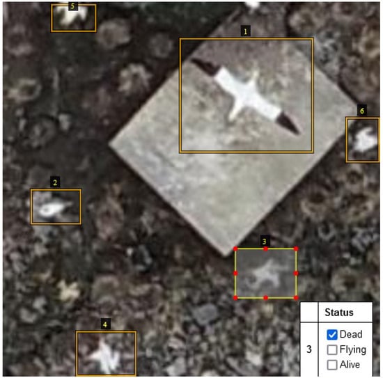
Figure 7.
Example of using the open source software VGG Image Annotator to classify gannets as either ‘Dead’ (e.g., box 3), ‘Alive’ (e.g., box 2), or ‘Flying’ (e.g., box 1). Nests and man-made structures are also visible.
Live and dead gannets exhibit distinct shapes: live gannets appear more ‘tucked in’ and elliptical, while dead gannets tend to have their wings and neck splayed out, providing a useful distinction for classification. To avoid misclassifying flying birds as ‘dead’ due to their spread wings, a separate class was added for flying birds (Figure 8). Flying birds appear larger in pixel size on the imagery, as they are closer to the drone camera, and it was expected that this information would help the model differentiate between the two classes.
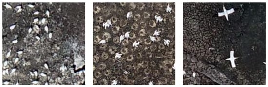
Figure 8.
200 × 200 pixel image tiles showing examples of the three classes of gannet; Left: live gannets on the ground appear elliptical in shape; Middle: dead gannets have their neck and wings splayed; Right: flying gannets appear larger with their wings evenly spread out.
Out of the 530 annotated tiles, 4496 were labelled as ‘Alive’, 1477 as ‘Dead’, and 313 as ‘Flying’. The annotated tile data were saved in a CSV file and read into the Python script. Rows without labels were removed, and the tile names, bounding box coordinates, and gannet status (Dead, Alive, Flying) were stored in a new file for the training process. For the model, ‘Dead’ were classified as 1, ‘Alive’ as 2, and ‘Flying’ as 3, with class 0 automatically assigned as a ‘background’ class.
2.2.3. Hyperparameters
There are several different hyperparameters that can be fine-tuned by the user when training the model, which are set before training begins. The values applied to this model are listed in Table 4. The final trained model was saved as a loadable file so that it could be easily applied to unseen datasets.
Table 4.
Hyperparameters fine-tuned for use in the model.
The optimal number of epochs for training the model was determined by assessing the loss function, which is an indicator of how good the model is at predicting the expected outcome, by observing the training loss and validation loss. Training loss is a metric used to evaluate model fitting on the training dataset (calculated by summing the errors on each individual image for each batch), while validation loss assesses model performance on the validation dataset (calculated by summing the errors on each individual image at the end of each epoch; []). The goal is to reach the lowest validation loss value to reduce overfitting. By plotting loss against training epochs, it is possible to determine if the model needs further fine-tuning to prevent under-fitting or over-fitting of the model. An optimal fit occurs when both training and validation loss decrease and stabilise at around the same epoch. In this model’s case, this occurred at epoch 15.
A section of code was added to automatically stop the training process when the validation loss reached a minimum value. If a lower value was not reached within 15 epochs, the process was terminated and the trained model at that minimum value was saved. This process is known as ‘early stopping’. The epoch at which the minimum was reached varied slightly each time the training process was executed (unless seeds are set), as it depends on which validation images the model utilises and other sources of randomness hidden in the model’s ‘black box’. Despite this, the minimum validation loss was always reached at approximately 4.2–4.7.
2.3. Validating the Model
To validate the model and see if it was working as expected, the remaining 53 of the 530 labelled image tiles were fed in and the output printed onto the screen.
2.3.1. Visualising Model Predictions
A function was created to draw coloured boxes around the gannets to highlight predictions made by the model for each validation tile. The red boxes indicate dead, blue boxes indicate alive, and yellow boxes indicate flying. A second function was used to draw pink boxes around birds manually labelled in VGG Image Annotator, known as the ‘ground-truth’ data. The goal was for all coloured boxes to lie on top of the pink boxes, indicating a correct prediction made by the model (Figure 9).
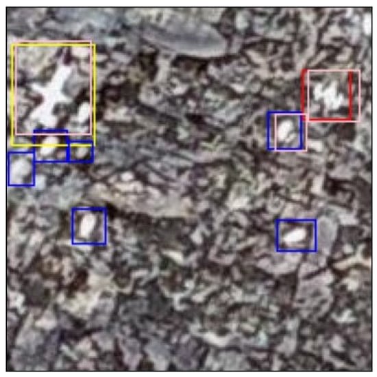
Figure 9.
200 × 200 pixel image tile showing example of ground-truth bounding boxes overlaid by predicted bounding boxes for each given class. Pink = ground truth, red = dead (class 1), blue = alive (class 2), yellow = flying (class 3). Any other background is class 0.
2.3.2. Model Performance Metrics
Positive and Negative Predictions
For object detection, it is important to determine the accuracy of both the resultant classifications and the position of the predicted bounding boxes compared to the ground truth. For the detections performed by the model, the resulting image tiles showed a combination of true positives, false positives, and false negatives—see Table 5 for definitions.
Table 5.
Definitions for object detection.
There are three different occurrences of FPs in the resultant images:
- Incorrect prediction made by the model, e.g., mistaking a rock for a bird (Figure 10).
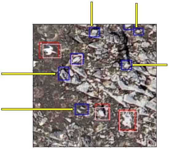 Figure 10. 200 × 200 pixel image tile showing examples of FP predictions made by the model that are rocks or other natural features, indicated by the yellow arrows.
 - Correct prediction of a bird by the model that was missed in the original labelling due to human error (Figure 11).
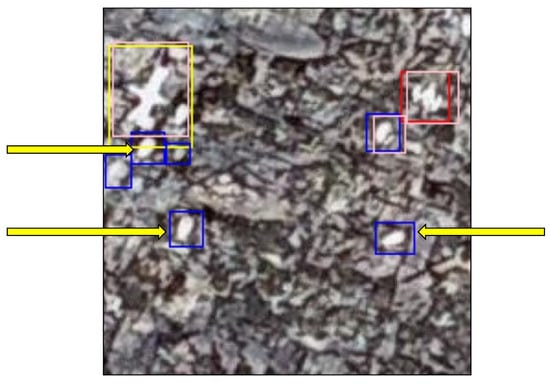 Figure 11. 200 × 200 pixel image tile showing examples of FP predictions made by the model that are real birds missed out of the ground truth, indicated by the yellow arrows. The arrows point to red/blue bounding boxes that do not have a pink ground-truth bounding box underneath.
 - Prediction made by the model, but the wrong classification given compared to ground truth.
The FN occurrences were far fewer and mostly occurred where two gannets were nesting close together, making it difficult for the model to tell them apart (Figure 12).
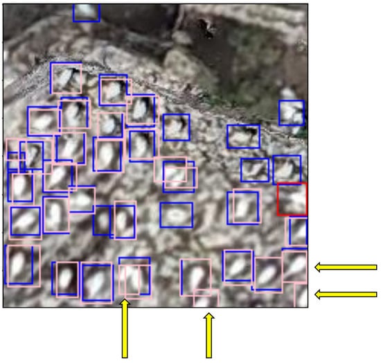
Figure 12.
200 × 200 pixel image tile showing examples of FN predictions made by the model, indicated by the yellow arrows. The arrows point to pink ground-truth bounding boxes that do not have an overlaying predicted red/blue bounding box.
Mean Average Precision (mAP)
An attempt was made to manually verify the predicted count and determine the accuracy of the model predictions compared to ground-truth data. Accuracy is usually calculated as the percentage of correct predictions out of all calculated predictions, given as:
However, this format is not reliable when analysing ‘class imbalanced’ data, where the number of bounding boxes provided for each class is different, as the output places a higher weight on learning those classes with more instances than those with less []. Instead, the mean Average Precision (mAP) is considered a better metric.
The mAP is a single value ranging from 0 to 1 that represents overall detection accuracy for an image (1 = 100% accuracy). The TorchMetrics function MeanAveragePrecision() (TorchMetrics, 2014) automatically calculates and utilises precision, recall, and AP based on the provided IoU threshold of 0.5, predicted bounding boxes/labels, and ground-truth bounding boxes/labels. As such, the mAP was calculated as 0.37 (37% accuracy), marking the final step in the model validation process. This aligns with the reported validation mAP of 32.8% for this model architecture, trained on the original COCO dataset by the PyTorch model developers [].
Reproducibility
To ensure reproducibility, three functions were added to the code to control sources of randomness that arise with each execution. This was performed by setting seed values. However, Pytorch states that complete reproducibility is not guaranteed across releases, commits, or platforms and that results may not be reproducible between CPU and GPU executions even when using identical seeds [].
The model was run three times on the 2022 dataset with three seed values set: torch.manual_seed(0), np.random.seed(0), and random_state = 1. The first two are set to minimise pseudo-randomness, while the latter ensures the same train-test split is used (i.e., the same 477 images are used for training and the same 53 images are used for validation). The results are listed in Table 6. While there is still some variation to be seen, it is not as large a difference as before the seed values were set, which could result in a difference of over 1000 live birds. Given the relatively poor contrast between rocks and birds in the 2022 dataset, this variation is deemed to be of an acceptable level.
Table 6.
Result of 3 model runs on the 2022 dataset to assess reproducibility when seed values are set.
3. Results
3.1. 2022 Dataset
3.1.1. Orthomosaic
An orthomosaic covering the full extent of Bass Rock was generated from 2022 drone imagery and immediately shows the impact of the HPAI outbreak—namely large swathes of bare ground where gannets previously would have been nesting (Figure 13). Remains of man-made structures are also visible, including the lighthouse, chapel, walled garden, foghorn, and walkways.
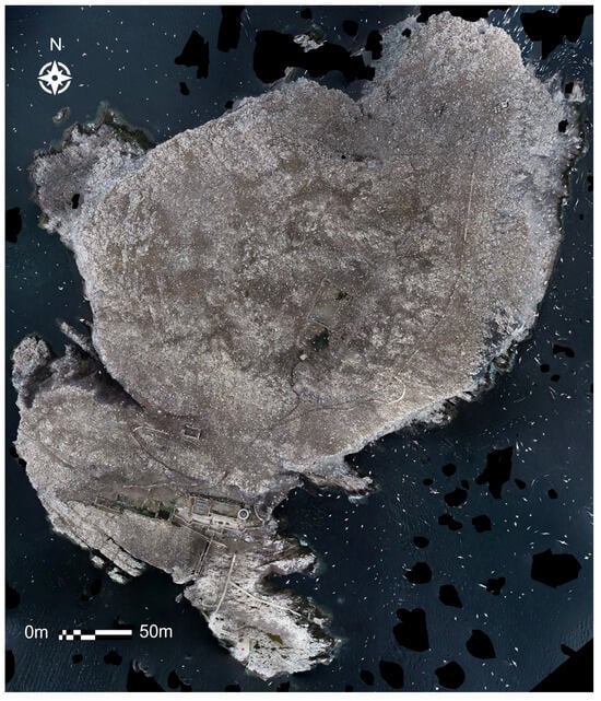
Figure 13.
Full orthomosaic generated from the 2022 RGB imagery.
3.1.2. 2022 Predicted Count
Since any FP predictions would end up included in the automatic count, the ‘true’ count was estimated. The FPs and FNs occurring for all three classes were manually counted in the 53 validation images using DotDotGoose, a free open-source tool to assist with manually counting objects in images ([]) A percentage change to apply to the entire dataset was then calculated by comparing the model count to the true count (TPs + FNs + misclassified FPs). The results are shown in Table 7.
Table 7.
Validating the predicted counts for the 2022 dataset. Model Count = counts predicted by model; FP(−) = FP predictions that were not birds (e.g., rocks); TP = TP predictions; FP(+) = misclassified FP predictions (e.g., predicted dead but actually alive); FN = FN predictions; True Count = total of TP, FP(+), and FN; % Change = difference between Model Count and True Count.
The fully trained and validated model was then run on the entire 2022 dataset consisting of 1481 image tiles. Table 8 shows the results of the predicted count for each of the three classes for the entire dataset.
Table 8.
Predicted counts for each class for the complete 2022 dataset.
3.1.3. Model vs. Manual Count
A manual count carried out by Glen Tyler at NatureScot predicted 21,277 live and 5053 dead gannets [], resulting in a 10% difference for combined live and flying gannets and 26% for dead gannets compared to the adjusted model predictions of 19,028 live (18,220 alive + 808 flying) and 4285 dead. The variation is likely due to the subjective nature of counting, along with challenges such as poor image quality, low colour contrast, and distorted imagery around rock edges, making accurate classifications and counts difficult.
3.2. 2023 Dataset
3.2.1. Orthomosaic
An orthomosaic covering the full extent of Bass Rock was generated from 2023 drone imagery (Figure 14). There are signs of initial population recovery, namely a higher density of gannets now occupying what was previously bare ground in Figure 13. However, it is still significantly below 2020 levels. The 2023 dataset showcased a marked increase in data quality thanks to the P1 camera, with individual gannets now more defined and feather colouration visible.
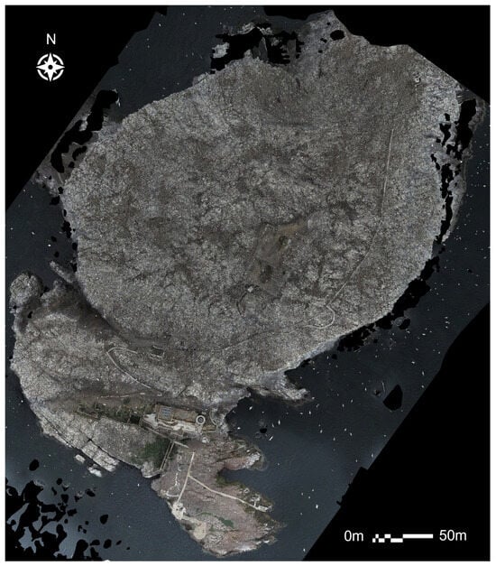
Figure 14.
Full orthomosaic generated from the 2023 RGB imagery.
3.2.2. 2023 Predicted Count
The saved, fully trained model from Section 2.2 was loaded and applied to all 1126 of the 500 × 500 pixel image tiles created in Section 2.1. Examples of the predictions are shown in Figure 15, Figure 16 and Figure 17.
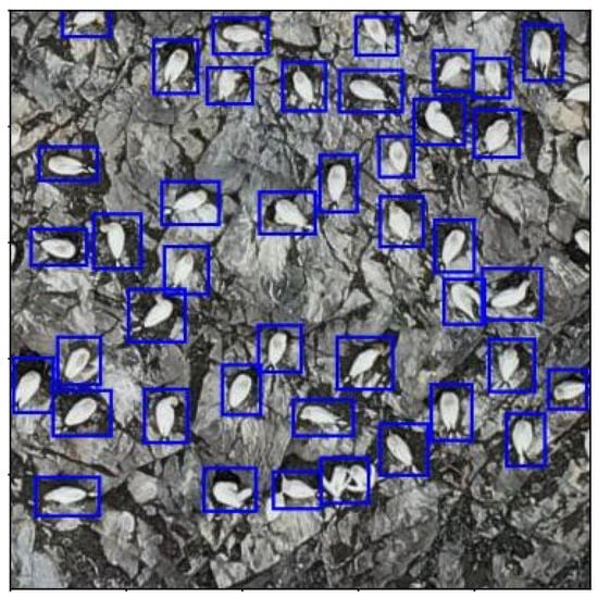
Figure 15.
500 × 500 pixel image tile showing examples of live model predictions (blue) from the 2023 dataset. Gannets clearly detected against rocky background.
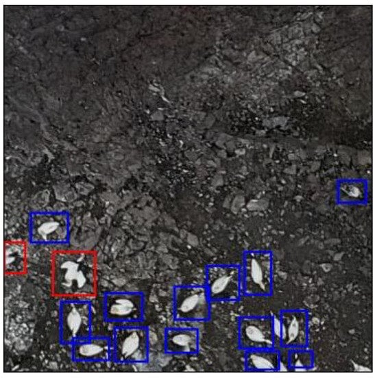
Figure 16.
500 × 500 pixel image tile showing examples of potential TP dead (left, red) and FP dead model predictions (right, red) from the 2023 dataset.
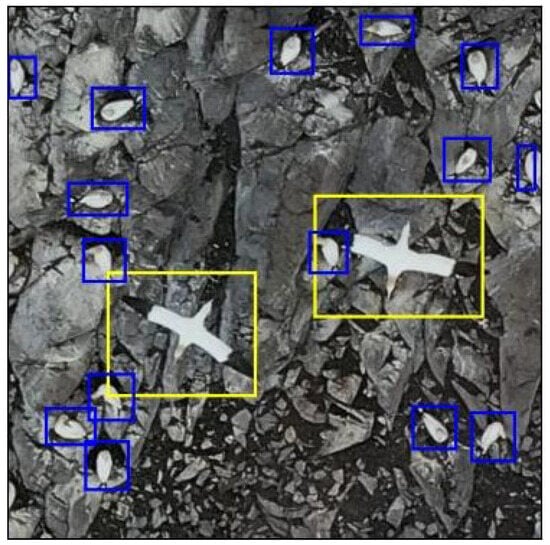
Figure 17.
500 × 500 pixel image tile showing examples of flying model predictions (yellow) from the 2023 dataset. Two gannets in flight clearly highlighted in contrast to live gannets on the ground.
Since the image quality is much greater than that of the 2022 dataset, the error on the predicted counts was re-estimated. A total of 165 of the predicted image tiles were saved and manually checked in DotDotGoose for FPs and FNs, and the appropriate adjustments to the counts were made (Table 9).
Table 9.
Validating the predicted counts for the 2022 dataset. Model Count = counts predicted by model; FP(−) = FP predictions that were not birds (e.g., rocks); TP = TP predictions; FP(+) = misclassified FP predictions (e.g., predicted dead but actually alive); FN = FN predictions; True Count = total of TP, FP(+), and FN; % Change = difference between Model Count and True Count.
The model was then run on the entire 2023 dataset, and the predicted counts were adjusted accordingly (Table 10).
Table 10.
Predicted counts for each class for the complete 2023 dataset.
3.2.3. Model vs. Manual Count
Comparison of Table 8 and Table 10 shows that there is an estimated increase in the number of live gannets for the assessed areas of 166% (2.5 times larger) from 2022 to 2023—a positive sign for its recovery. Three independent manual counts of individuals were carried out using DotDotGoose [] by the UKCEH and the Scottish Seabird Centre. An average was taken for the three counters to provide a final value of 51,428 live birds (not including those in flight), marking a 6% difference between the model count and the manual count. Very few birds were classed as dead, with a mean of 23.
4. Discussion
The project aimed to utilise a deep learning neural network to automate the detection and counting of northern gannets in drone imagery of Bass Rock from 2022 and 2023. The analysis covered nine of the counting areas marked out in Figure 1 (1, 2, 3, 8 + 9, 10, 11, 12, 13) and part of one more (7). The areas in Figure 1 not assessed here (4, 5, 6) are those that could not be covered by the drone due to line-of-sight restrictions. These areas relate to sheer cliff faces where the gannets are known to nest. In 2014, when coverage of the colony was complete, these missing areas contained 15.4% of the population []. In this way, the results presented here do not offer a complete census of the entirety of the Bass Rock gannetry.
When applied to the 2022 dataset, the DL model predicted 18,220 live and 3761 dead gannets, which closely aligns with NatureScot’s manual count of 21,277 live and 5035 dead gannets []. Subsequently, the model was applied to the 2023 dataset and predicted 48,455 live and only 43 dead gannets. In terms of the number of gannets associated with Bass Rock in 2023, these results show a substantial increase of 166% compared to the same areas imaged in 2022. The manual count for 2023 provided a number of 51,428 live gannets. If we assume the manual count to be the ‘ground truth’, then the model performed with around 95% accuracy compared to counting manually.
To enhance the comparability of the estimated count provided in this study with previous Bass Rock censuses, it would be advantageous for future research to investigate the model’s capability or adaptability to estimate Apparently Occupied Sites (AOSs), a metric conventionally employed previously. Deriving AOSs from an individual live bird count necessitates a context-dependent conversion factor, with anticipated variations across colonies, years, and different seasonal periods. Therefore, this study also serves as an initial effort towards developing an automated count of AOSs.
4.1. Limitations
4.1.1. Labelling and Classification
The model output relies heavily on training data quality, and poor class representation can result from an inadequate amount of labelling or incorrect bird classification—the result of a subjective process. To mitigate this, it is recommended to agree with experienced counters on what represents live or dead birds in imagery and to ensure that similar numbers of labelled examples are made for each class—though the model does account for ‘class imbalance’ to some extent through calculation of the mAP.
In the 2023 dataset, the model predicted 1510 dead gannets, with 97% estimated to be FPs. After discussion, it was decided that some of the remaining 3% were probably also alive, and some were likely to really be dead (Figure 18). It was also apparent that many of the FN predictions in both datasets occurred when two gannets were sat very close together, e.g., on a nest, which the model could not easily separate.
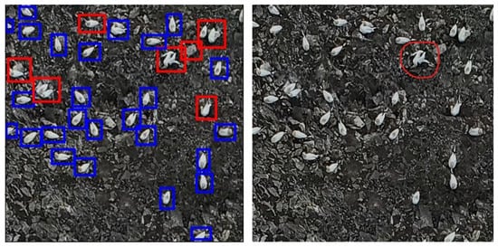
Figure 18.
500 × 500 pixel image tiles showing examples of dead predictions made by the model (Left, red boxes), and the potential TP dead prediction (Right, red circle).
It is important to note that from an aerial perspective, the posture of a dead gannet can appear very similar to one that is ‘displaying’, which presents uncertainty for this particular classification. As such, if a rapid and accurate assessment of mortality is required, then it is vital to try to improve the identifying criteria to distinguish between dead and displaying gannets through more rigorous ground truthing in conjunction with behavioural experts.
Due to the increased resolution of the P1 camera, it might be worth re-training the model using the higher-quality 2023 dataset to see if gannets close together could be better resolved as separate individuals. However, it should be noted that while models trained on ‘worse’ data will run well on better quality data, the reverse is not true. For example, an attempt was made to run the model on historical Bass Rock survey data from 2014, but the poorer quality, motion blur, and viewing angle meant that it did not work effectively enough to be of any use.
The model should ideally be trained using hundreds of images to increase classification representation, but the sizes of the datasets used here were limiting. A way to solve this would be to implement ‘data augmentation’, which artificially increases the size and robustness of the training dataset by making adjustments to copies of the labelled images by, e.g., rotating, resizing, flipping, or changing the brightness [].
4.1.2. Model Performance
The mAP acquired on the 2022 dataset of 37% is in line with the value of 32.8% expected from using Pytorch’s pre-trained Faster R-CNN MobileNetv3-Large FPN architecture. As mentioned in Section 2.2.1, the model was ‘downgraded’ from the suggested ResNet50 due to the available GPU. Had that been used, then the mAP would have increased to around 46.7% []. Pre-training the model with a dataset other than MS COCO may also help with increasing the mAP, as COCO mostly consists of images taken at a regular/side-on viewing angle, whereas the data used here are top-down.
Implementing a different DL architecture and running on a larger GPU could offer improvements in terms of computational efficiency and prediction accuracy. On top of this, pre-training on a different dataset than MS COCO may also offer an improvement.
4.2. Outcomes
4.2.1. Population Counts
In the 2022 dataset, the model and manual counts differed by 10% for live birds and 26% for dead birds. This discrepancy might be due to the lower quality of the imagery, making it challenging to make the same subjective classifications. The 2022 adjustment values in Table 8 are much lower than those calculated for the 2023 data in Table 10, as the model performs better on data with known features used during training, such as pixel size, noise, brightness, and contrast. Similar to Hayes et al. [], this study also found that FPs were the most common prediction errors by the model.
In the 2023 dataset, the model significantly overestimated dead birds and underestimated flying birds, potentially because of the P1 camera’s higher resolution, which can sometimes misinterpret the shape of a live bird on the ground. For example, after visiting Bass Rock in person, it was noted that live gannets stand up and fan their wings out when defending their space, which can be misinterpreted as being a ‘dead’ shape when viewed from above. The expertise of the Scottish Seabird Centre was important in identifying likely TP predictions for dead gannets, which is a crucial factor to get right during an HPAI outbreak scenario.
Image overlap during stitching of the orthomosaic could lead to the same bird being counted multiple times, particularly with flying birds. Flying gannets were often missed as FNs rather than being misclassified. Occasionally, the model also picked up herring gulls, but there were not enough instances to determine if it was a sporadic prediction accident or if a larger number of them would require separate classification.
4.2.2. Deep Learning Model
The Faster R-CNN MobileNetv3-Large FPN architecture provided a streamlined system for quick performance on both GPU and CPU (Section 4.2.3). Another study, published online, also uses the Faster R-CNN MobileNetv3-Large FPN model for bird species detection using Pytorch and DL. However, it uses regular ‘side-on’ images of birds and is applied to species recognition only, not counting [].
The DL model performed well and achieved 37% accuracy, though some manual verification is still required to fine-tune this. This performance aligns with Hong et al. [], where they also used a Faster R-CNN DL model to detect birds from drone imagery at a 100 m flight height. Despite using a larger dataset and ResNet backbone, with the birds on arguably less complex terrain, the results here share similar positive aspects of speed and accuracy. A similar issue of sensitivity to the bounding box pixel size was noted in their study, which was addressed in this work by resizing the 2023 image tiles.
Although Hong et al. [] conclude that they are currently gathering aerial imagery of dead birds to develop a more robust model, there is currently nothing in the literature where this has previously been done. This makes the study presented here one of the first to do so.
4.2.3. Time Efficiency
One of the main aims was to see if it were possible to significantly reduce the time required to acquire a population estimate. The results of this are described in Table 11.
Table 11.
Description of how the DL model reduces time requirements.
Using the saved trained model, obtaining an initial predicted total count takes less than 2 min. Data preparation for the model, including generating the orthomosaic and image tiles, is also relatively quick, at about 1 h. Compared to the current manual methodology [], this approach significantly saves time and provides an instantaneous overview of the colony’s well-being. If needed, manual verification can still be performed using the saved imagery containing the model predictions.
Similarly, Kellenberger et al. [] reported that their CNN model for detecting terns and gulls reduced analysis time from a few days to a few hours, with the prediction stage only taking a few minutes. However, they did not utilise early stopping and ran the model for 75 epochs, visually ensuring convergence, which increased training time to over 3 h. This study demonstrates that implementing early stopping can greatly minimise the required run time.
5. Conclusions
The combination of drone-based remote sensing and deep learning provides a swift and adaptable method for accurately monitoring the northern gannet population on Bass Rock. This methodology improves upon the labour-intensive manual counts based on aerial digital photography first used by Murray et al. [], representing the first advancement of the survey process in almost 15 years.
The results presented here are the first known application of deep learning to detect dead birds from drone imagery with the specific aim of quantifying the impact of HPAI on a bird colony. The model’s potential extends to other gannet colonies in the UK and, with some re-training, could be adapted to detect other bird species, making it a valuable tool for conservation purposes.
Author Contributions
Conceptualisation, A.A.T., C.J.N., T.W. and E.B.; Data curation, A.A.T. and T.W.; Formal analysis, A.A.T.; Investigation, A.A.T.; Methodology, A.A.T. and S.P.; Project administration, C.J.N. and E.B.; Resources, T.W.; Software, S.P.; Supervision, C.J.N.; Validation, A.A.T., M.P.H., S.W. and E.B.; Visualisation, A.A.T.; Writing—original draft, A.A.T.; Writing—review and editing, C.J.N., M.P.H., S.W. and E.B. All authors have read and agreed to the published version of the manuscript.
Funding
A.A.T. acknowledges the University of Edinburgh’s School of Geosciences field costs as part of the MSc Earth Observation & Geoinformation Management programme.
Data Availability Statement
The datasets presented in this article are not readily available because the data are part of an ongoing study. Requests to access the datasets should be directed to caroline.nichol@ed.ac.uk.
Acknowledgments
Thank you to Susan Davies and Maggie Sheddon at the Scottish Seabird Centre for sharing their intimate knowledge of gannet behaviour and for facilitating our trips onto Bass Rock. Thank you to Stuart Murray of Murray Survey who provided the previous decadal census counts, and to Sue Lewis of Edinburgh Napier University for her contribution to the manual count. In Memoriam: Professor Mike Harris: The authors, as well as wider colleagues at the University of Edinburgh, the Scottish Seabird Centre and the UK Centre for Ecology and Hydrology, were extremely saddened to hear of the passing of our co author and colleague, Professor Mike Harris, following the submission of this paper. Mike was a world leader in seabird science and conservation, and enjoyed a long and highly successful career. Mike was instrumental in pioneering the aerial census of northern gannet colonies around the UK and Ireland, and we will remain indebted to him for his valuable collaboration to this work, which he remained excited and committed to, up until his death. We dedicate this publication to his memory.
Conflicts of Interest
The authors declare no conflicts of interest.
References
- Rush, G.P.; Clarke, L.E.; Stone, M.; Wood, M.J. Can drones count gulls? Minimal disturbance and semiautomated image processing with an unmanned aerial vehicle for colony-nesting seabirds. Ecol. Evol. 2018, 8, 12322–12334. [Google Scholar] [CrossRef]
- Conservation from the Clouds: The Use of Drones in Conservation. 2022. Available online: https://www.gwct.org.uk/blogs/news/2022/october/conservation-from-the-clouds-the-use-of-drones-in-conservation/ (accessed on 24 February 2023).
- Raudino, H.C.; Tyne, J.A.; Smith, A.; Ottewell, K.; McArthur, S.; Kopps, A.M.; Chabanne, D.; Harcourt, R.G.; Pirotta, V.; Waples, K. Challenges of collecting blow from small cetaceans. Ecosphere 2019, 10, e02901. [Google Scholar] [CrossRef]
- Sellés-Ríos, B.; Flatt, E.; Ortiz-García, J.; García-Colomé, J.; Latour, O.; Whitworth, A. Warm beach, warmer turtles: Using drone-mounted thermal infrared sensors to monitor sea turtle nesting activity. Front. Conserv. Sci. 2022, 3, 954791. [Google Scholar] [CrossRef]
- Lane, J.V.; Jeglinski, J.W.; Avery-Gomm, S.; Ballstaedt, E.; Banyard, A.C.; Barychka, T.; Brown, I.H.; Brugger, B.; Burt, T.V.; Careen, N.; et al. High Pathogenicity Avian Influenza (H5N1) in Northern Gannets (Morus bassanus): Global Spread, Clinical Signs and Demographic Consequences. Ibis. Available online: https://onlinelibrary.wiley.com/doi/pdf/10.1111/ibi.13275 (accessed on 22 September 2023). [CrossRef]
- Avian Flu. 2022. Available online: https://www.rspb.org.uk/birds-and-wildlife/advice/how-you-can-help-birds/disease-and-garden-wildlife/avian-influenza-updates (accessed on 4 April 2023).
- Murray, S.; Harris, M.P.; Wanless, S. The status of the Gannet in Scotland in 2013–14. Scott. Birds 2015, 35, 3–18. [Google Scholar]
- Bass Rock SSSI. 2022. Available online: https://sitelink.nature.scot/site/155 (accessed on 15 February 2023).
- Murray, S.; Wanless, S.; Harris, M. The Bass Rock—Now the world’s largest Northern Gannet colony. Br. Birds 2014, 107, 769–770. [Google Scholar]
- Seabirds on the Brink as Avian Flu Rips through Colonies for a Third Year. 2023. Available online: https://www.rspb.org.uk/about-the-rspb/about-us/media-centre/press-releases/seabirds-on-the-brink-as-avian-flu-rips-through-colonies-for-a-third-year/ (accessed on 29 July 2023).
- Murray, S.; Wanless, S.; Harris, M. The status of the Northern Gannet in Scotland 2003–04. Scott. Birds 2006, 26, 17–29. [Google Scholar]
- Sardà-Palomera, F.; Bota, G.; Viñolo, C.; Pallarés, O.; Sazatornil, V.; Brotons, L.; Gomáriz, S.; Sardà, F. Fine-scale bird monitoring from light unmanned aircraft systems. Ibis 2012, 154, 177–183. [Google Scholar] [CrossRef]
- Hodgson, J.C.; Baylis, S.M.; Mott, R.; Herrod, A.; Clarke, R.H. Precision wildlife monitoring using unmanned aerial vehicles. Sci. Rep. 2016, 6, 22574. [Google Scholar] [CrossRef]
- Chabot, D.; Craik, S.R.; Bird, D.M. Population Census of a Large Common Tern Colony with a Small Unmanned Aircraft. PLoS ONE 2015, 10, e0122588. [Google Scholar] [CrossRef]
- What Are Neural Networks? 2023. Available online: https://www.ibm.com/topics/neural-networks (accessed on 1 May 2023).
- Wäldchen, J.; Mäder, P. Machine learning for image based species identification. Methods Ecol. Evol. 2018, 9, 2216–2225. [Google Scholar] [CrossRef]
- Kellenberger, B.; Veen, T.; Folmer, E.; Tuia, D. 21,000 birds in 4.5 h: Efficient large-scale seabird detection with machine learning. Remote. Sens. Ecol. Conserv. 2021, 7, 445–460. [Google Scholar] [CrossRef]
- Akçay, H.G.; Kabasakal, B.; Aksu, D.; Demir, N.; Öz, M.; Erdoğan, A. Automated Bird Counting with Deep Learning for Regional Bird Distribution Mapping. Animals 2020, 10, 1207. [Google Scholar] [CrossRef] [PubMed]
- Hayes, M.C.; Gray, P.C.; Harris, G.; Sedgwick, W.C.; Crawford, V.D.; Chazal, N.; Crofts, S.; Johnston, D.W. Drones and deep learning produce accurate and efficient monitoring of large-scale seabird colonies. Ornithol. Appl. 2021, 123, duab022. [Google Scholar] [CrossRef]
- Hong, S.J.; Han, Y.; Kim, S.Y.; Lee, A.Y.; Kim, G. Application of Deep-Learning Methods to Bird Detection Using Unmanned Aerial Vehicle Imagery. Sensors 2019, 19, 1651. [Google Scholar] [CrossRef] [PubMed]
- Dujon, A.M.; Ierodiaconou, D.; Geeson, J.J.; Arnould, J.P.Y.; Allan, B.M.; Katselidis, K.A.; Schofield, G. Machine learning to detect marine animals in UAV imagery: Effect of morphology, spacing, behaviour and habitat. Remote Sens. Ecol. Conserv. 2021, 7, 341–354. Available online: https://onlinelibrary.wiley.com/doi/pdf/10.1002/rse2.205 (accessed on 12 June 2023). [CrossRef]
- Kuru, K.; Clough, S.; Ansell, D.; McCarthy, J.; McGovern, S. WILDetect: An intelligent platform to perform airborne wildlife census automatically in the marine ecosystem using an ensemble of learning techniques and computer vision. Expert Syst. Appl. 2023, 231, 120574. [Google Scholar] [CrossRef]
- Bist, R.B.; Subedi, S.; Yang, X.; Chai, L. Automatic Detection of Cage-Free Dead Hens with Deep Learning Methods. AgriEngineering 2023, 5, 1020–1038. [Google Scholar] [CrossRef]
- Geldart, E.A.; Barnas, A.F.; Semeniuk, C.A.; Gilchrist, H.G.; Harris, C.M.; Love, O.P. A colonial-nesting seabird shows no heart-rate response to drone-based population surveys. Sci. Rep. 2022, 12, 18804. [Google Scholar] [CrossRef]
- Irigoin-Lovera, C.; Luna, D.M.; Acosta, D.A.; Zavalaga, C.B. Response of colonial Peruvian guano birds to flying UAVs: Effects and feasibility for implementing new population monitoring methods. PeerJ 2019, 7, e8129. [Google Scholar] [CrossRef]
- Brisson-Curadeau, E.; Bird, D.; Burke, C.; Fifield, D.A.; Pace, P.; Sherley, R.B.; Elliott, K.H. Seabird species vary in behavioural response to drone census. Sci. Rep. 2017, 7, 17884. [Google Scholar] [CrossRef]
- Edney, A.; Hart, T.; Jessopp, M.; Banks, A.; Clarke, L.; Cugniere, L.; Elliot, K.; Juarez Martinez, I.; Kilcoyne, A.; Murphy, M.; et al. Best practices for using drones in seabird monitoring and research. Mar. Ornithol. 2023, 51, 265–280. [Google Scholar]
- Orthomosaic & DEM Generation (without GCPs). 2023. Available online: https://agisoft.freshdesk.com/support/solutions/articles/31000157908-orthomosaic-dem-generation-without-gcps (accessed on 20 January 2023).
- ArcGIS Pro. 2023. Available online: https://www.esri.com/en-us/arcgis/products/arcgis-pro/overview (accessed on 1 January 2023).
- Faster R-CNN: Model Builders. 2023. Available online: https://pytorch.org/vision/stable/models/faster_rcnn.html (accessed on 2 May 2023).
- Howard, A.G.; Zhu, M.; Chen, B.; Kalenichenko, D.; Wang, W.; Weyand, T.; Andreetto, M.; Adam, H. MobileNets: Efficient Convolutional Neural Networks for Mobile Vision Applications. arXiv 2017, arXiv:1704.04861. [Google Scholar]
- Lin, T.Y.; Maire, M.; Belongie, S.; Hays, J.; Perona, P.; Ramanan, D.; Dollár, P.; Zitnick, C.L. Microsoft COCO: Common Objects in Context. In Computer Vision—ECCV 2014, Proceedings of the 13th European Conference, Zurich, Switzerland, 6–12 September 2014; Fleet, D., Pajdla, T., Schiele, B., Tuytelaars, T., Eds.; Lecture Notes in Computer Science; Springer: Cham, Switzerland, 2014. [Google Scholar]
- Dutta, A.; Gupta, A.; Zissermann, A. VGG Image Annotator (VIA). Version: 2.0.8. 2016. Available online: http://www.robots.ox.ac.uk/~vgg/software/via/ (accessed on 24 February 2023).
- Understanding Learning Rate. 2019. Available online: https://bit.ly/3rB2jzW (accessed on 13 June 2023).
- The Difference between a Batch and an Epoch in a Neural Network. 2022. Available online: https://machinelearningmastery.com/difference-between-a-batch-and-an-epoch/ (accessed on 13 June 2023).
- Training and Validation Loss in Deep Learning. 2023. Available online: https://www.baeldung.com/cs/training-validation-loss-deep-learning (accessed on 21 July 2023).
- Evaluating Object Detection Models: Guide to Performance Metrics. 2019. Available online: https://manalelaidouni.github.io/Evaluating-Object-Detection-Models-Guide-to-Performance-Metrics.html#intersection-over-union-iou (accessed on 23 May 2023).
- Models and Pre-Trained Weights. 2023. Available online: https://pytorch.org/vision/stable/models.html (accessed on 21 July 2023).
- Reproducibility. 2023. Available online: https://pytorch.org/docs/stable/notes/randomness.html (accessed on 12 June 2023).
- DotDotGoose (v.1.6.0). 2023. Available online: https://biodiversityinformatics.amnh.org/open_source/dotdotgoose (accessed on 30 June 2023).
- A Complete Guide to Data Augmentation. 2023. Available online: https://www.datacamp.com/tutorial/complete-guide-data-augmentation (accessed on 21 July 2023).
- Bird Species Detection Using Deep Learning and PyTorch. 2023. Available online: https://debuggercafe.com/bird-species-detection-using-deep-learning-and-pytorch/ (accessed on 20 July 2023).
Disclaimer/Publisher’s Note: The statements, opinions and data contained in all publications are solely those of the individual author(s) and contributor(s) and not of MDPI and/or the editor(s). MDPI and/or the editor(s) disclaim responsibility for any injury to people or property resulting from any ideas, methods, instructions or products referred to in the content. |
© 2024 by the authors. Licensee MDPI, Basel, Switzerland. This article is an open access article distributed under the terms and conditions of the Creative Commons Attribution (CC BY) license (https://creativecommons.org/licenses/by/4.0/).