Robust Flight-Path Angle Consensus Tracking Control for Non-Minimum Phase Unmanned Fixed-Wing Aircraft Formation in the Presence of Measurement Errors

Abstract

The robust flight-path angle consensus tracking control problem for multiple unmanned fixed-wing aircrafts is investigated in this paper, where the non-minimum phase properties and the presence of measurement errors are systematically addressed. A three-module control scheme is proposed for each aircraft: a Distributed Observer that obtains the available information from the reference system and the neighbor aircraft to provide the estimates of the reference states; a Casual Stable Inversion that calculates the bounded estimates of the desired input, desired external states, and most importantly, desired internal states to resolve the divergence issues caused by the non-minimum phase properties; and a Local Measurement Error Rejection Controller that includes a measurement error estimator (MEE) to actively compensate for the adverse effect of measurement errors to achieve robust consensus tracking control. Stability, convergence, and robustness of the proposed control are analyzed, showing that (1) the non-minimum phase issue can be systematically resolved by the designed Casual Stable Inversion to ensure aircraft internal stability and flight safety, and (2) the consensus tracking accuracy can be improved by tuning a single MEE parameter, which is favorable in practical applications to large-scale unmanned aircraft formations. Comparative simulation results with classic PID-based consensus control demonstrate the advantage of the proposed control in transient oscillations, steady-state tracking accuracy, and robustness against measurement errors.

1. Introduction

Formation control of unmanned fixed-wing aircrafts has received considerable attention in the past decades, as it holds promise for extending the capability of a single aircraft to satisfy the growing demand for complex flight missions at a large scale, such as aerial surveillance [1], monitoring [2], search [3], target tracking [4], and so on. As one fundamental control mode in these missions, flight-path angle consensus tracking control achieves motion synchronization of the unmanned aircraft during the climb [5], steady wing-level flight, and landing [6]. However, compared with consensus control of other aircraft states (such as pitch angle, angle of attack, velocity, or height), flight-path angle consensus control is much more challenging due to the inherent non-minimum phase properties of the flight-path angle dynamics. Specifically, for the conventional unmanned fixed-wing aircraft longitudinal model, one real open right half-plane zero (sometimes called the “non-minimum phase zero”) exists in the input–output relationship between the elevator deflection and flight-path angle [7], rendering the corresponding internal dynamics unstable. If the internal dynamics stabilization is not considered in the output tracking control design for non-minimum phase systems, the internal states will almost certainly diverge to destabilize the whole system. Unfortunately, most existing consensus control and consensus tracking control methods (such as [8,9,10,11,12,13,14]) assume the controlled system to be minimum-phase or have no internal dynamics. These methods can hardly be applied to the considered problem in this paper.

To the best of the author’s knowledge, only a handful of works in the literature deal with the problem of consensus control of non-minimum phase systems. Work [15] presents a pole-placement-based distributed adaptive output consensus control scheme for heterogeneous non-minimum phase multi-agent systems in a leader-follower manner, to address the issues of unknown agent parameters and unknown non-identical relative degrees. A low-gain feedback consensus protocol is proposed in [16] for non-minimum phase discrete-time linear multi-agent systems, to achieve output consensus to the optimal point that minimizes the overall objective function, within any specified consensus error. In [17], a two-term control law is proposed for non-linear non-minimum phase multi-agent systems, where a local term stabilizes the internal dynamics, and a coupling term guarantees output consensus. A Lyapunov-like function-based time-dependent switching law is proposed in [18] to ensure state-stabilization of a class of non-minimum phase non-linear systems with switched dynamics. The non-uniform and unknown delays in the consensus control problem of multiple heterogeneous general linear systems are considered in [19], and a pre-filter is utilized to shape the dynamics of the agent that are stabilized by a local feedback controller, such that the consensus condition is satisfied. Work [20] presents an output redefinition-based control method for non-linear non-minimum phase multi-agent systems to achieve output consensus while stabilizing the internal dynamics.

One important limitation of the methods proposed in the aforementioned works, however, lies in the fact that only output consensus is considered in the design, whereas the output tracking of a reference can hardly be achieved. This restricts the application of these methods to the considered problem, because flight-path angle consensus tracking control, instead of consensus control, is generally required in real flight missions to achieve the path-following of certain desired trajectories. To guarantee accurate output consensus tracking for multiple non-minimum phase systems, an iterative output redefinition-based method is proposed in [21], which overcomes the inherent tracking accuracy limitation of classic output redefinition methods. In [22], this goal is attained by employing a distributed iterative learning control based on the successive projection framework that ensures the satisfaction of the system constraints. In contrast, an inversion-based control approach is proposed in [23], where a causal stable inversion module uses local and neighbors’ information from the distributed observer network to calculate the estimates of the bounded input and state reference for the controller, such that the output tracking and internal dynamics stabilization are simultaneously delivered.

Another practically important issue for aircraft control is measurement error rejection. The measurement errors, when brought to the closed-loop system by the feedback control, can degrade the control accuracy, wear the actuator, and even cause instability [24]. However, none of the above works takes measurement error rejection into account in the control design, and the related discussions in the literature are few. The measurement errors are considered in the non-minimum-phase multi-agent system output consensus control problem in [25,26], but the measurement errors and external disturbances are assumed to be generated by the states of the same exosystem. This assumption may be impractical in the sense that measurement errors and external disturbances can exhibit completely different frequency characteristics, and thus, they cannot, in most cases, be described based on a single exosystem model. From the above observations, the consensus tracking control of multiple non-minimum phase systems in the presence of measurement errors, as well as its application to fixed-wing aircraft, are still open to be investigated.

In this paper, a three-module control scheme is developed to deal with the flight-path angle consensus tracking control problem for multiple unmanned fixed-wing aircraft. The modules Distributed Observer, Casual Stable Inversion, and Local Measurement Error Rejection Controller achieve distributed reference system estimation, bounded estimation of desired input and state for internal dynamics stabilization, and robust measurement error rejection tracking control, respectively. The novelties and contributions of this paper are summarized as follows.

• Regarding the consensus control of multiple non-minimum phase systems, compared with the existing approaches (such as [15,16,17,18,19,20]) that are only capable of achieving output consensus with perfect measurements, the proposed approach is the first attempt to systematically resolves the output consensus tracking and the measurement error rejection problems simultaneously. Moreover, this paper shows the application of the proposed approach to the flight-path angle consensus tracking for multiple unmanned fixed-wing aircrafts;
• The separation property of the proposed three-module control scheme allows it to be easily modified and adapted to other robust or optimal consensus tracking control problems of non-minimum phase unmanned aircraft formations or heterogeneous unmanned aircraft formations;
• As proved theoretically and verified by simulations, a single parameter $T_{ni}$ in the proposed Local Measurement Error Rejection Controller determines the system robustness against measurement errors and the overall control accuracy. This property makes parameter tuning easier and more intuitive than other approaches involving multi-parameter tuning and optimization, especially for formations of large numbers of unmanned aircraft.

The rest of this paper is organized as follows. Section 2 formulates the flight-path angle consensus tracking control problem for multiple unmanned fixed-wing aircraft, where the aircraft model, communication topology, and control objectives are described. Section 3 presents the proposed control scheme with the detailed designs of the three modules Distributed Observer, Casual Stable Inversion, and Local Measurement Error Rejection Controller. Stability, convergence, and robustness analysis is provided in Section 4, and the theoretical analysis results are further verified by numerical simulations in Section 5. Finally, the conclusions are drawn in Section 6.

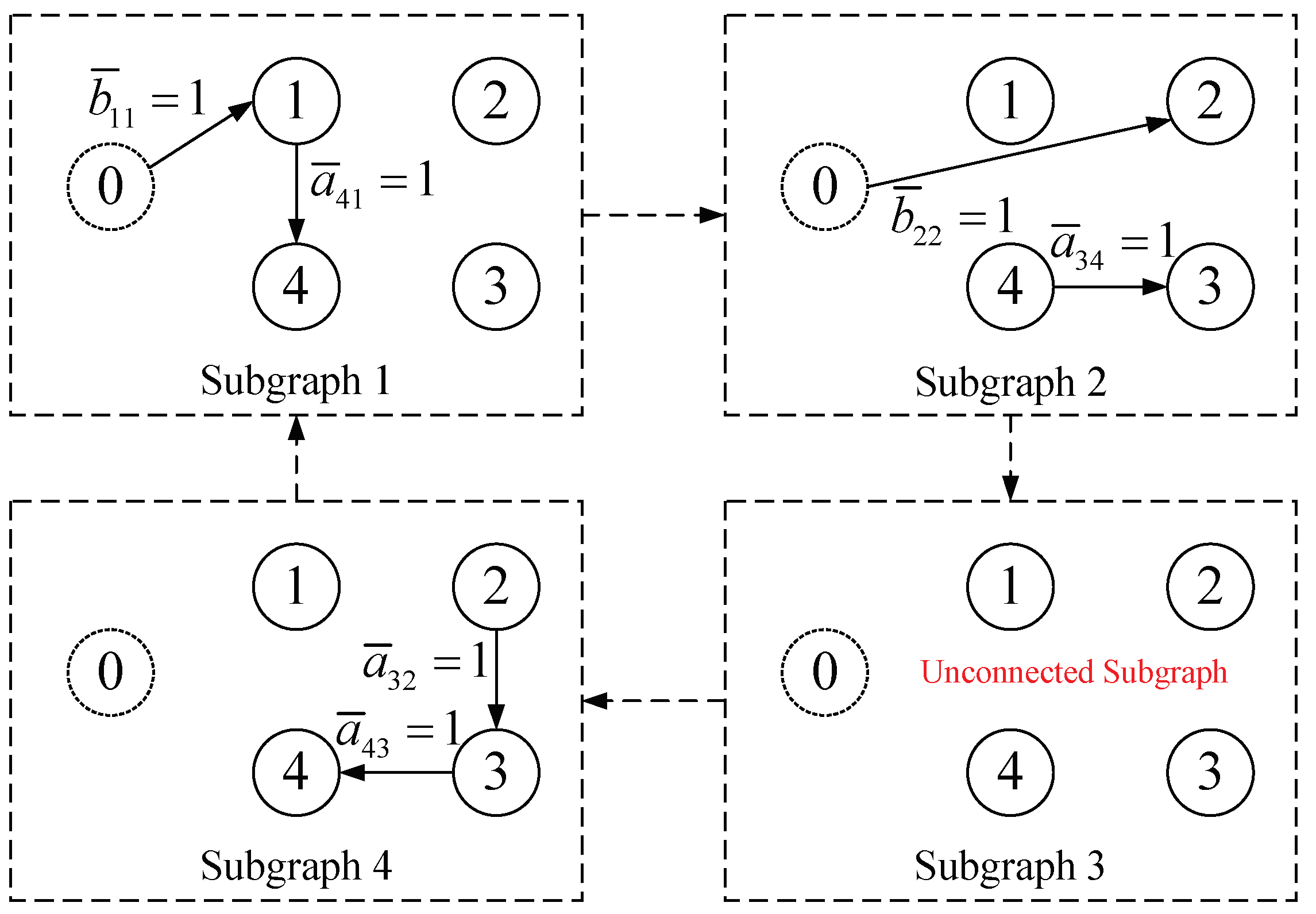
2. Problem Formulation

In this section, the modeling of the flight-path angle motion of an unmanned fixed-wing aircraft is first presented, followed by the description of the considered consensus tracking control problem of multiple aircraft in the presence of measurement errors.

The linearized longitudinal dynamics of conventional unmanned fixed-wing aircraft can be expressed in a state-space form as:

$$\begin{array}{ccc}\hfill \left[\begin{array}{c}\dot{\alpha }\\ \dot{q}\\ \dot{\theta }\end{array}\right]& =& \underset{{\mathit{A}}_o}{\underbrace{\left[\begin{array}{ccc}{a}_{11}& a_{12}& 0\\ a_{21}& a_{22}& 0\\ 0& 1& 0\end{array}\right]}}\underset{{\mathit{x}}_o}{\underbrace{\left[\begin{array}{c}\alpha \\ q\\ \theta \end{array}\right]}}+\underset{{\mathit{B}}_o}{\underbrace{\left[\begin{array}{c}{b}_1\\ b_2\\ 0\end{array}\right]}}{\delta }_e,\hfill \\ \hfill y& =& \underset{{\mathit{C}}_o}{\underbrace{\left[\begin{array}{ccc}-1& 0& 1\end{array}\right]}}{\mathit{x}}_o,\hfill \\ \hfill {\mathit{y}}_s& =& {\mathit{x}}_o+\mathit{n},\hfill \end{array}$$

(1)

where $\alpha \in \mathbb{R}$ denotes the angle of attack, $q\in \mathbb{R}$ denotes the body-axis pitch rate, $\theta \in \mathbb{R}$ denotes the pitch angle, ${\delta }_e\in \mathbb{R}$ is the system input, denoting the elevator deflection angle, the system output is the flight-path angle denoted by $y=\gamma =\theta -\alpha$, and ${\mathit{y}}_s$ is the measured output with measurement error $\mathit{n}$.

Assumption 1.

${∥\mathit{n}\left(t\right)∥}_2$ is bounded for all $t\ge 0$.

According to Section 3.1.2 of [27], the normal form (in which the internal states are not explicitly driven by the control inputs) of system (1) can be obtain by applying a non-singular linear transformation matrix $\mathit{T}\in {\mathbb{R}}^{3\times 3}$ to system (1). Specifically, applying the following coordinate transformation matrix:

$$\mathit{T}=\left[\begin{array}{ccc}-1& 0& 1\\ 1& -\frac{b_1}{b_2}& 0\\ 0& 0& 1\end{array}\right]$$

(2)

to the original state ${\mathit{x}}_o$ generates a new state vector:

$${\mathit{x}}_T=\mathit{T}{\mathit{x}}_o={\left[\begin{array}{cc}\gamma & {\mathsf{\eta }}^T\end{array}\right]}^T,$$

(3)

where $\gamma$ is the external state and $\mathsf{\eta }\in {\mathbb{R}}^2$ is the internal state. Suppose $b_1\ne 0$ and $b_2\ne 0$ are true under all flight conditions, which is reasonable in the sense that $b_1=b_2=0$ renders the aircraft uncontrollable. Then, it is clear that the transformation matrix (3) is non-singular. In the new coordinate, the system matrix and input matrix satisfy:

$$\begin{array}{ccc}\hfill {\mathit{A}}_T& =& \mathit{T}{\mathit{A}}_o{\mathit{T}}^{-1},\hfill \\ \hfill {\mathit{B}}_T& =& \mathit{T}{\mathit{B}}_o,\hfill \end{array}$$

(4)

where ${\mathit{A}}_T$ can be partitioned into four $2\times 2$ blocks as:

$${\mathit{A}}_T=\left[\begin{array}{cc}{A}_{\gamma }& {\mathit{A}}_{\eta }\\ \mathit{G}& \mathit{D}\end{array}\right],A_{\gamma }\in \mathbb{R},{\mathit{A}}_{\eta }\in {\mathbb{R}}^{1\times 2},\mathit{G}\in {\mathbb{R}}^{2\times 1},\mathit{D}\in {\mathbb{R}}^{2\times 2},$$

(5)

and ${\mathit{B}}_T$ is expressed explicitly as:

$${\mathit{B}}_T={\left[\begin{array}{ccc}{b}_{T1}& 0& 0\end{array}\right]}^T,b_{T1}\in \mathbb{R}.$$

(6)

The original system model (1) has now been converted into its “normal form” as:

$$\begin{array}{ccc}\hfill {\dot{\mathit{x}}}_T& =& {\mathit{A}}_T{\mathit{x}}_T+{\mathit{B}}_T{\delta }_e,\hfill \\ \hfill y& =& \left[\begin{array}{ccc}1& 0& 0\end{array}\right]{\mathit{x}}_T.\hfill \end{array}$$

(7)

Based on the feedback linearization technique, the virtual input is defined as:

$$u=A_{\gamma }\gamma +{\mathit{A}}_{\eta }\mathit{\eta }+b_{T1}{\delta }_e,$$

(8)

then, the original input ${\delta }_e$ can be calculated from the virtual input u and the new state vector ${\mathit{x}}_T$:

$${\delta }_e=\frac{1}{b_{T1}}(u-A_{\gamma }\gamma -{\mathit{A}}_{\eta }\mathit{\eta }).$$

(9)

With (8), the normal form (7) can be further rewritten as:

$$\begin{array}{ccc}\hfill \dot{\gamma }& =& u,\hfill \end{array}$$

(10)

$$\begin{array}{ccc}\hfill \dot{\mathit{\eta }}& =& \mathit{D}\mathit{\eta }+\mathit{G}\gamma ,\hfill \end{array}$$

(11)

where (10) denotes the external dynamics and (11) denotes the internal dynamics. It is observed from the above equations that in the normal form, the external state $\gamma$ is driven explicitly by the virtual input u, whereas the internal state $\mathit{\eta }$ is not directly controlled by u, but is driven by the external state $\gamma$.

We employ the following assumptions for the internal dynamics (11):

Assumption 2.

$\mathit{D}$ has at least one right half plane pole, and $\mathit{D}$ is non-singular.

Assumption 3.

The pair $(\mathit{D},\mathit{G})$ is stabilizable.

The statement “$\mathit{D}$ has at least one right half plane pole” in Assumption 2 limits the discussion of this paper to a non-minimum phase unmanned fixed-wing aircraft, and the statement “$\mathit{D}$ is non-singular” ensures the solvability of the bounded particular solution of the unstable internal dynamics with a casual output reference. Meanwhile, Assumption 3 ensures the stabilizablity of the internal dynamics and the solvability of the considered control problem.

The state-space equations of (10) and (11) is written as:

$$\begin{array}{ccc}\hfill \dot{\mathit{x}}& =& \mathit{A}\mathit{x}+\mathit{B}u,\hfill \\ \hfill y& =& \mathit{C}\mathit{x},\hfill \end{array}$$

(12)

where the state vector satisfies $\mathit{x}={\mathit{x}}_T={\left[\begin{array}{cc}\gamma & {\mathit{\eta }}^T\end{array}\right]}^T$, and the system matrix, input matrix, and the output matrix are, respectively, given by:

$$\mathit{A}=\left[\begin{array}{cc}0& {\mathbf{0}}_{1\times 2}\\ \mathit{G}& \mathit{D}\end{array}\right],\mathit{B}=\left[\begin{array}{c}1\\ {\mathbf{0}}_{2\times 1}\end{array}\right],\mathit{C}=\left[\begin{array}{ccc}1& 0& 0\end{array}\right].$$

(13)

It is worth noting that the original and new state-space Equations (1) and (12) share the same output $y=\gamma$, the flight-path angle, but have different inputs.

In what follows, the consensus tracking control problem is formulated. To start with, a group of $N\in \mathbb{R}$ aircraft is considered, and we define:

$$\mathcal{N}=\{1,2,\dots ,N\}.$$

(14)

To permit an application to a group of aircraft, the subscript “i” is added to each variable (including the states, input, output, and other related variables such as measurement error $\mathit{n}$ and internal state $\mathit{\eta }$) of the aircraft model. Then, the original model (1) for the group is rewritten as:

$$\begin{array}{ccc}\hfill {\dot{\mathit{x}}}_{o_i}& =& {\mathit{A}}_o{\mathit{x}}_{o_i}+{\mathit{B}}_o{\delta }_{e_i},\hfill \\ \hfill y_i& =& {\mathit{C}}_o{\mathit{x}}_{o_i},\hfill \\ \hfill {\mathit{y}}_{s_i}& =& {\mathit{x}}_{o_i}+{\mathit{n}}_i,i\in \mathcal{N},\hfill \end{array}$$

(15)

to which, when the coordinate transformation (2) is applied, the following normal form expressed in the new coordinate is obtained:

$$\begin{array}{ccc}\hfill {\dot{\mathit{x}}}_i& =& \mathit{A}{\mathit{x}}_i+\mathit{B}{u}_i,\hfill \\ \hfill y_i& =& \mathit{C}{\mathit{x}}_i,i\in \mathcal{N}.\hfill \end{array}$$

(16)

Suppose the desired output $y_{di}$ for each aircraft is generated by the same reference system to achieve consensus output tracking control. Define the reference system as:

$$\begin{array}{ccc}\hfill {\dot{\mathit{z}}}_d& =& {\mathit{A}}_d{\mathit{z}}_d,\hfill \\ \hfill y_{di}& =& {\mathit{C}}_d{\mathit{z}}_d,\hfill \end{array}$$

(17)

where ${\mathit{z}}_d\in {\mathbb{R}}^2$ is the state of the reference system, $y_{di}={\gamma }_{di}\in \mathbb{R}$ is the desired flight-path angle for i-th aircraft, and ${\mathit{A}}_d\in {\mathbb{R}}^{2\times 2}$ and ${\mathit{C}}_d\in {\mathbb{R}}^{2\times 1}$ are the state matrix and output matrix of the reference system, respectively. To ensure the boundedness of the reference signal, ${\mathit{A}}_d$ is selected to be Hurwitz.

To describe the communication topology among the union of the aircraft group (15) and the reference system (17), the following switching graph:

$$\overline{\mathcal{G}}\left(t\right)=\{\overline{\mathcal{V}},\overline{\mathcal{E}}\left(t\right)\}$$

(18)

is introduced, where the i-th aircraft is denoted by a node $v_i$, and the reference system is denoted by the node $v_0$. Use $\overline{\mathcal{V}}=\{v_1,v_2,\dots ,v_N,v_0\}$ to denote the node set that includes the reference system, $\overline{\mathcal{E}}\left(t\right)\subseteq \left\{(v_i,v_j)\right|v_i,v_j\in \overline{\mathcal{V}}\}$ to denote the edge set which may switch from time to time. Then, the directed edge ${\overline{e}}_{ij}\left(t\right)$ indicates that the information of node $v_j$ is accessible to its neighbor node $v_i$ at time t. The adjacency matrix and Laplacian matrix of graph $\overline{\mathcal{G}}\left(t\right)$ is denoted by $\overline{\mathit{A}}\left(t\right)\in {\mathbb{R}}^{N\times N}$ and $\overline{\mathit{L}}\left(t\right)\in {\mathbb{R}}^{N\times N}$, respectively, where ${\overline{a}}_{ij}\left(t\right)=1$ if ${\overline{e}}_{ij}\left(t\right)\in \mathcal{E}\left(t\right)$, and otherwise ${\overline{a}}_{ij}\left(t\right)=0$. Define $\overline{\mathit{B}}\left(t\right)=diag\left\{{\overline{b}}_{ii}\left(t\right)\right\}\in {\mathbb{R}}^{N\times N}$ to describe the information interaction between each aircraft and the reference, where ${\overline{b}}_{ii}\left(t\right)=1$ if ${\overline{e}}_{i0}\left(t\right)\in \mathcal{E}\left(t\right)$, indicating that the i-th aircraft can access the reference system at time t, and otherwise ${\overline{b}}_{ii}\left(t\right)=0$. To ensure the information reachability of the group, the following assumption on $\overline{\mathcal{G}}\left(t\right)$ is imposed.

Assumption 4

(Assumption 5 in [28]). There exists a subsequence $\left\{i_k\right\}$ of $\left\{i\right|i=0,1,\dots \}$ with $t_{i_{k+1}}-t_{i_k}<\tau$ for some positive τ such that every node is reachable from the reference $v_0$ in the union graph ${\bigcup }_{j=i_k}^{i_{k+1}-1}\overline{\mathcal{G}}\left(t\right)$.

Figure 1 demonstrates one possible switching communication topology satisfying Assumption 4, which allows one or some of the subgraphs to be unconnected.

The control objective of this paper is to design a robust consensus tracking controller ${\delta }_{e_i}$ for each aircraft in the group using its own and its neighbors’ information.

(i-a) Asymptotic consensus tracking: the flight-path angle ${\gamma }_i$ of each aircraft tracks asymptotically the desired output ${\gamma }_{di}$ generated by the reference system (17), namely:

$$\underset{t\to \infty }{lim}\left|{\gamma }_{di}\left(t\right)-{\gamma }_i\left(t\right)\right|=0,\forall i\in \mathcal{N},$$

(19)

provided that the measurement error satisfies ${\mathit{n}}_i={\mathbf{0}}_{3\times 1}$;

(i-b) Approximate consensus tracking: ${\gamma }_i$ tracks ${\gamma }_{di}$ within an specified error, i.e.,

$$\left|{\gamma }_{di}\left(t\right)-{\gamma }_i\left(t\right)\right|\le {\varsigma }_i,\forall t\ge t_{{\varsigma }_i},\forall i\in \mathcal{N},$$

(20)

when ${\mathit{n}}_i\ne {\mathbf{0}}_{3\times 1}$, where ${\varsigma }_i>0$ is a constant, representing the specified ultimate bound of the tracking error $\left|{\gamma }_{di}\left(t\right)-{\gamma }_i\left(t\right)\right|$, and $t_{{\varsigma }_i}>0$ is the settling time;

(ii) Internal state stabilization: the state ${\mathit{x}}_{o_i}$ and the internal state ${\mathit{\eta }}_i$ satisfy:

$$\parallel {\mathit{x}}_{o_i}\left(t\right)\parallel <\infty ,\parallel {\mathit{\eta }}_i\parallel <\infty ,\forall t\ge 0,\forall i\in \mathcal{N}.$$

(21)

In the above objectives, the consensus tracking performance is quantized by the objective (19) in the absence of measurement error, and the ultimate bound ${\varsigma }_i$ in (20) specifies the robustness of the controller against measurement errors. Meanwhile, the objective (21) is essential for the considered non-minimum phase system to ensure that the unstable internal dynamics are appropriately stabilized.

3. Control Design

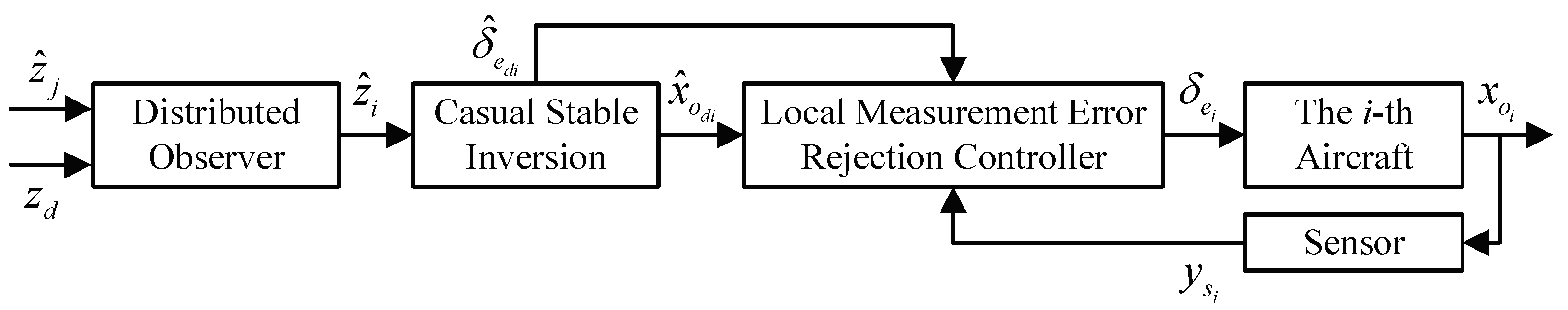
3.1. Overall Control Scheme

In this paper, a three-module control scheme is proposed for i-th aircraft shown in Figure 2. Specifically, by using the available information ${\mathit{z}}_d$ and ${\widehat{\mathit{z}}}_j$ from the reference system (17) and its neighbors, the Distributed Observer of i-th aircraft generates the estimate of ${\mathit{z}}_d$, denoted by ${\widehat{\mathit{z}}}_j$, from which the Casual Stable Inversion calculates the feedforward control term ${\widehat{\delta }}_{e_{di}}$ and the state reference ${\widehat{\mathit{x}}}_{o_{di}}$ expressed in the original coordinate system (1) for the controller. Then, the Local Measurement Error Rejection Controller generates the elevator deflection control command ${\delta }_{e_i}$ that achieves robust trajectory tracking of the reference using noisy output feedback signal $y_{s_i}$ obtained from the sensors. The design of each module will be detailed in what follows.

3.2. Design of the Distributed Observer

The role of Distributed Observer is to provide Casual Stable Inversion with the asymptotic estimation of the reference system (17) under a switching and possibly occasionally disconnected communication topology. The Distributed Observer for the i-th aircraft in the group is designed as:

$$\begin{array}{ccc}\hfill {\dot{\widehat{\mathit{z}}}}_i\left(t\right)& =& {\mathit{A}}_d{\widehat{\mathit{z}}}_i\left(t\right)+l_i{\mathit{e}}_i\left(t\right),\hfill \\ \hfill {\mathit{e}}_i\left(t\right)& =& {\overline{b}}_{ii}\left(t\right)[{\mathit{z}}_d\left(t\right)-{\widehat{\mathit{z}}}_i\left(t\right)]+\sum _{j\in \mathcal{N}}{\overline{a}}_{ij}\left(t\right)[{\widehat{\mathit{z}}}_j\left(t\right)-{\widehat{\mathit{z}}}_i\left(t\right)],i\in \mathcal{N},\hfill \end{array}$$

(22)

where ${\widehat{\mathit{z}}}_i\in {\mathbb{R}}^2$ is the state of the Distributed Observer and $l_i\in \mathbb{R}$ is the observer feedback gain. The feedback term ${\mathit{e}}_i\left(t\right)$ consist of two components: the first component ${\overline{b}}_{ii}\left(t\right)[{\mathit{z}}_d\left(t\right)-{\widehat{\mathit{z}}}_i\left(t\right)]$ drives the Distributed Observer to synchronize its state ${\widehat{\mathit{z}}}_i$ with the reference system state ${\mathit{z}}_d$ when the reference information is accessible, i.e., when ${\overline{b}}_{ii}\left(t\right)\ne 0$; the second component ${\displaystyle \sum _{j\in \mathcal{N}}}{\overline{a}}_{ij}\left(t\right)[{\widehat{\mathit{z}}}_j\left(t\right)-{\widehat{\mathit{z}}}_i\left(t\right)]$ is to achieve synchronization of the state of the Distributed Observer of the i-th aircraft with that of its neighbors.

Based on the reference system model (17), the desired flight-path angle for the i-th aircraft can be calculated from the Distributed Observer (22) as:

$${\widehat{\gamma }}_{di}={\mathit{C}}_d{\widehat{\mathit{z}}}_{di}.$$

(23)

Since the controlled system (16) is of non-minimum phase, simply designing an output feedback controller that tracks the output reference (23) for system (16) can lead to the divergence of the unstable internal dynamics (11). To stabilize the internal dynamics, an internal-state feedback control component should be employed in addition to the output tracking controller. Therefore, the idea of the proposed control scheme is to convert the original output tracking problem into a full-state tracking problem, such that not only the output tracking, but also the internal dynamics stabilization, are simultaneously achieved. To design a full-state feedback controller, the key problem is to calculate the state reference from the Distributed Observer (22), which will be discussed in the following section.

3.3. Design of the Casual Stable Inversion

For the i-th aircraft expressed in the new coordinate (16), respectively, define its desired state and input that correspond to its desired output $y_{di}$ given by (17) as ${\mathit{x}}_{di}$ and $u_{di}$, which satisfy the following dynamics:

$$\begin{array}{ccc}\hfill {\dot{\mathit{x}}}_{di}& =& \mathit{A}{\mathit{x}}_{di}+\mathit{B}{u}_{di},\hfill \\ \hfill y_{di}& =& \mathit{C}{\mathit{x}}_{di}.\hfill \end{array}$$

(24)

The process of using $y_{di}$ and (24) to calculate ${\mathit{x}}_{di}$ and $u_{di}$ is called “Inversion”. The major difficulty of such process lies in the fact that the non-minimum phase property of (16) renders its inversion dynamics unstable, since the unstable zero in (16) becomes the unstable pole in the inversion system. If the calculated ${\mathit{x}}_{di}$ and $u_{di}$ become unbounded, the controller can generate unbounded control signal that renders the system states divergent. Therefore, it is necessary to calculate the bounded particular solution of ${\mathit{x}}_{di}$ and $u_{di}$, denoted, respectively, by ${\mathit{x}}_{di}^{\ast }$ and $u_{di}^{\ast }$, from system (24). This calculation process is also known as finding the “ideal internal dynamics” [29] or “stable inversion” [30].

However, classic stable inversion-based approaches require the output reference ${\gamma }_d$ to be a non-causal signal, whereas in this paper, this requirement is not satisfied due to two facts. First, the output reference ${\gamma }_d$ for each aircraft is not prior known, but is obtained online by the Distributed Observer, making the reference a causal signal. Second, since the subgraphs of the switching communication topology can be unconnected, the output reference might not be available to some of the aircraft in the formation at certain times, and thus, obtaining a non-causal reference signal is impossible in the considered formation control problems. The requirement is only satisfied in the extreme case where every aircraft in the formation is informed with the full knowledge of the reference system before formation flights are taken place, but this case, it is not practically meaningful because no cooperative action is needed for the formation to achieve consensus trajectory tracking. In this paper, to overcome the limitation of classic approaches, a Casual Stable Inversion module is designed that only uses the casual reference signals generated by the Distributed Observer to calculate the asymptotic estimates of the bounded particular solution in real-time.

In what follows, the state of the Distributed Observer (22) is used to first calculate the estimate of the desired input ${\widehat{u}}_{di}$, and then, the estimate of the desired state ${\widehat{\mathit{x}}}_{di}$ is constructed based on casual stable inversion technique. From (10) and (17), the desired input is readily obtained by:

$$u_{di}={\dot{\gamma }}_{di}={\mathit{C}}_d{\mathit{A}}_d{\mathit{z}}_{di},$$

(25)

and along with (23), the estimate of the desired input is designed as:

$${\widehat{u}}_{di}={\dot{\widehat{\gamma }}}_{di}={\mathit{C}}_d{\mathit{A}}_d{\widehat{\mathit{z}}}_{di}.$$

(26)

The estimate of the desired state ${\widehat{\mathit{x}}}_{di}$ can be expressed in a partitioned vector form as:

$${\widehat{\mathit{x}}}_{di}={\left[\begin{array}{cc}{\widehat{\gamma }}_{di}& {\widehat{\mathit{\eta }}}_{di}^T\end{array}\right]}^T,$$

(27)

where ${\widehat{\gamma }}_{di}$ is already given by (23) and ${\widehat{\mathit{\eta }}}_{di}\in {\mathbb{R}}^2$ is the estimates of the desired internal state ${\mathit{\eta }}_{di}$. To ensure the boundedness of ${\widehat{\mathit{\eta }}}_{di}$, the following virtual dynamics are constructed that ${\widehat{\mathit{\eta }}}_{di}$ satisfies:

$${\dot{\widehat{\mathit{\eta }}}}_{di}=\mathit{D}{\widehat{\mathit{\eta }}}_{di}+\mathit{G}{\widehat{\gamma }}_{di}+{\mathit{g}}_i,i\in \mathcal{N},$$

(28)

where ${\mathit{g}}_i\in {\mathbb{R}}^2$ are auxiliary functions to render (28) globally input-to-state stable. According to [31], ${\mathit{g}}_i$ can be designed as:

$${\ddot{\widehat{\mathit{\eta }}}}_i+p_1{\dot{\widehat{\mathit{\eta }}}}_i+p_0{\widehat{\mathit{\eta }}}_i={\mathit{F}}_1{\dot{\mathit{g}}}_i+{\mathit{F}}_0{\mathit{g}}_i,i\in \mathcal{N},$$

(29)

where $p_0$ and $p_1$ are the coefficients of the characteristic polynomial of ${\mathit{A}}_d$ in the reference system (17) given by:

$$P\left(s\right)=s^2+p_{1}s+p_0,$$

(30)

and ${\mathit{F}}_0\in {\mathbb{R}}^{2\times 2}$ and ${\mathit{F}}_1\in {\mathbb{R}}^{2\times 2}$ satisfy:

$$\begin{array}{ccc}\hfill {\mathit{F}}_0& =& c_0({\mathit{I}}_2-{\mathit{F}}_1){\mathit{D}}^{-1}-p_0{\mathit{D}}^{-1},\hfill \\ \hfill {\mathit{F}}_1& =& {\mathit{I}}_2-({\mathit{I}}_2+p_1{\mathit{D}}^{-1}+p_0{\mathit{D}}^{-2})({\mathit{I}}_2+c_1{\mathit{D}}^{-1}+c_0{\mathit{D}}^{-2}),\hfill \end{array}$$

(31)

where $c_0>0$ and $c_1>0$ determines the convergence speed of ${\mathit{g}}_i\to {\mathbf{0}}_{2\times 1}$, and ${\mathit{I}}_2$ is the $2\times 2$ identity matrix. In the rest of this paper, the notation ${\mathit{I}}_N$ is used to denote the identity matrix of N-th order. Plugging (28) into (29) eliminates ${\mathit{g}}_i$ to obtain the dynamics of ${\widehat{\mathit{\eta }}}_i$ as:

$${\ddot{\widehat{\mathit{\eta }}}}_i+c_1{\dot{\widehat{\mathit{\eta }}}}_i+c_0{\widehat{\mathit{\eta }}}_i=-({\mathit{P}}_1\mathit{G}{\dot{\widehat{\gamma }}}_{di}+{\mathit{P}}_0\mathit{G}{\widehat{\gamma }}_{di}),i\in \mathcal{N},$$

(32)

where ${\dot{\widehat{\gamma }}}_{di}={\widehat{u}}_{di}$, and ${\mathit{P}}_0\in {\mathbb{R}}^{2\times 2}$ and ${\mathit{P}}_1\in {\mathbb{R}}^{2\times 2}$ satisfy:

$$\begin{array}{ccc}\hfill {\mathit{P}}_0& =& c_0{\mathit{D}}^{-1}-({\mathit{P}}_1+I_2)p_0{\mathit{D}}^{-1},\hfill \\ \hfill {\mathit{P}}_1& =& ({\mathit{I}}_2+c_1{\mathit{D}}^{-1}+c_0{\mathit{D}}^{-2}){({\mathit{I}}_2+p_1{\mathit{D}}^{-1}+p_0{\mathit{D}}^{-2})}^{-1}-{\mathit{I}}_2.\hfill \end{array}$$

(33)

By running the virtual dynamics (32), each aircraft is able to solve ${\widehat{\mathit{\eta }}}_{di}$ from ${\widehat{\gamma }}_{di}$ and ${\widehat{u}}_{di}$ given by (23) and (26). Up to now, the estimates of desired input, state, and output (denoted, respectively, by ${\widehat{u}}_{di}$, ${\widehat{\mathit{x}}}_{di}$, and ${\widehat{\gamma }}_{di}$) have been derived based on the new coordinate (12). The next step is to convert them back into the original coordinate (1). Define ${\delta }_{e_{di}}$ and ${\mathit{x}}_{o_{di}}$ as the desired input and state in the original coordinate, respectively, then from (9) and (3) we have:

$$\begin{array}{ccc}\hfill {\delta }_{e_{di}}& =& \frac{1}{b_{T1}}(u_{di}-{\mathit{A}}_{ext}{\mathit{x}}_{di}),\hfill \\ \hfill {\mathit{x}}_{o_{di}}& =& {\mathit{T}}^{-1}{\mathit{x}}_{di},\hfill \end{array}$$

(34)

where

$${\mathit{A}}_{ext}=\left[\begin{array}{cc}{A}_{\gamma }& {\mathit{A}}_{\eta }\end{array}\right]\in {\mathbb{R}}^{3\times 1}$$

(35)

denotes the system matrix of the external states. For each aircraft, it is natural to replace $u_d$ and ${\mathit{x}}_d$ in (34) with their estimates ${\widehat{u}}_{di}$ and ${\widehat{\mathit{x}}}_{di}$, respectively, to obtain:

$$\begin{array}{ccc}\hfill {\widehat{\delta }}_{e_{di}}& =& \frac{1}{b_{T1}}({\widehat{u}}_{di}-{\mathit{A}}_{ext}{\widehat{\mathit{x}}}_{di}),\hfill \\ \hfill {\widehat{\mathit{x}}}_{o_{di}}& =& {\mathit{T}}^{-1}{\widehat{\mathit{x}}}_{di},i\in \mathcal{N},\hfill \end{array}$$

(36)

which are regarded as the outputs of the Casual Stable Inversion.

3.4. Design of the Local Measurement Error Rejection Controller

In this section, a measurement error estimator (MEE)-based robust controller is developed to achieve not only trajectory tracking but also measurement error rejection. Specifically, the MEE is designed based on the closed-loop model to generate the measurement error estimation signal, by which the controller could employ a corresponding compensation signal to cancel out the adverse effects of measurement errors. By this idea, the local robust controller for the i-th aircraft is designed as:

$${\delta }_{e_i}={\widehat{\delta }}_{e_{di}}+{\mathit{K}}_i({\widehat{\mathit{x}}}_{o_{di}}-{\mathit{y}}_{s_i}+{\widehat{\mathit{n}}}_i),i\in \mathcal{N},$$

(37)

where the feedforward signal ${\widehat{\delta }}_{e_{di}}$ and the state reference ${\widehat{\mathit{x}}}_{o_{di}}$ are generated by the Casual Stable Inversion, ${\mathit{K}}_i=\left[\begin{array}{ccc}{k}_{1i}& k_{2i}& k_{3i}\end{array}\right]$ is the feedback gain matrix and ${\widehat{\mathit{n}}}_i$ is the estimate of the measurement error ${\mathit{n}}_i$ generated by MEE. In the frequency domain, MEE is designed to satisfy:

$${\widehat{\mathit{N}}}_i\left(s\right)=G_{ni}\left(s\right){\mathit{N}}_i\left(s\right),i\in \mathcal{N}$$

(38)

where $G_{ni}\left(s\right)$ is a proper stable transfer function, which represents one design freedom of MEE. Combining (15), (37) and (38) yields:

$${\widehat{\mathit{N}}}_i\left(s\right)=G_{ni}\left(s\right)[{\mathit{Y}}_{s_i}\left(s\right)-{(s{\mathit{I}}_3-{\mathit{A}}_o)}^{-1}[{\mathit{B}}_o{\widehat{\delta }}_{e_{di}}\left(s\right)+{\mathit{B}}_o{\mathit{K}}_i[{\widehat{\mathit{X}}}_{o_{di}}\left(s\right)-{\mathit{Y}}_{s_i}\left(s\right)+{\widehat{\mathit{N}}}_i\left(s\right)]+{\mathit{x}}_{o_i}\left(0\right)]],$$

(39)

from which solving ${\widehat{\mathit{N}}}_i\left(s\right)$ gives the following explicit form of MEE:

$${\widehat{\mathit{N}}}_i\left(s\right)={\overline{\mathit{G}}}_{ni}\left(s\right)[{\mathit{Y}}_{s_i}\left(s\right)-{\mathit{P}}_o[{\widehat{\delta }}_{e_{di}}\left(s\right)+{\mathit{K}}_i[{\widehat{\mathit{X}}}_{o_{di}}\left(s\right)-{\mathit{Y}}_{s_i}\left(s\right)]]],$$

(40)

where

$${\mathit{P}}_o\left(s\right)={(s{\mathit{I}}_3-{\mathit{A}}_o)}^{-1}{\mathit{B}}_o=\left[\begin{array}{c}\frac{b_{1}s+a_{12}{b}_2-a_{22}{b}_1}{s^2-(a_{11}+a_{22})s+(a_{11}{a}_{22}-a_{12}{a}_{21})}\\ \frac{b_{2}s-a_{11}{b}_2+a_{21}{b}_1}{s^2-(a_{11}+a_{22})s+(a_{11}{a}_{22}-a_{12}{a}_{21})}\\ \frac{b_{2}s-a_{11}{b}_2+a_{21}{b}_1}{s^3-(a_{11}+a_{22})s^2+(a_{11}{a}_{22}-a_{12}{a}_{21})s}\end{array}\right],$$

(41)

$${\overline{\mathit{G}}}_{ni}\left(s\right)=G_{ni}\left(s\right){[{\mathit{I}}_3+G_{ni}\left(s\right){(s{\mathit{I}}_3-{\mathit{A}}_o)}^{-1}{\mathit{B}}_o{\mathit{K}}_i]}^{-1}.$$

(42)

It is worth mentioning that the initial condition term ${\mathit{x}}_{o_i}\left(0\right)$ is neglected in MEE design (40), since this term cannot be measured precisely in the presence of measurement errors. The neglect of ${\mathit{x}}_{o_i}\left(0\right)$ can cause an estimation error given by:

$$\begin{array}{cc}\hfill & G_{ni}\left(s\right){(s{\mathit{I}}_3-{\mathit{A}}_o)}^{-1}{\mathit{x}}_{o_i}\left(0\right)\hfill \\ \hfill & =G_{ni}\left(s\right)\left[\begin{array}{c}\frac{{\alpha }_i\left(0\right)s+(-a_{22}{\alpha }_i\left(0\right)+a_{12}{q}_i\left(0\right))}{s^2-(a_{11}+a_{22})s+(a_{11}{a}_{22}-a_{12}{a}_{21})}\\ \frac{q_i\left(0\right)s+(a_{21}{\alpha }_i\left(0\right)-a_{11}{q}_i\left(0\right))}{s^2-(a_{11}+a_{22})s+(a_{11}{a}_{22}-a_{12}{a}_{21})}\\ \frac{{\theta }_i\left(0\right)s^2+(q_i\left(0\right)-a_{11}{\theta }_i\left(0\right)-a_{22}{\theta }_i\left(0\right))s+(a_{21}{\alpha }_i\left(0\right)-a_{11}{q}_i\left(0\right)+a_{11}{a}_{22}{\theta }_i\left(0\right)-a_{12}{a}_{21}{\theta }_i\left(0\right))}{s^3-(a_{11}+a_{22})s^2+(a_{11}{a}_{22}-a_{12}{a}_{21})s}\end{array}\right],\hfill \end{array}$$

(43)

where

$${\mathit{x}}_{o_i}\left(0\right)={\left[\begin{array}{ccc}{\alpha }_i\left(0\right)& q_i\left(0\right)& {\theta }_i\left(0\right)\end{array}\right]}^T$$

(44)

is the initial state. According to [32], to asymptotically eliminate the adverse effect caused by (43), the transfer function $G_{ni}\left(s\right)$ should include at least one differentiator “s” in its numerator to cancel out the integrator “$\frac{1}{s}$” existing in (43), and thus, $G_{ni}\left(s\right)$ can be selected as the following first-order high-pass filter:

$$G_{ni}\left(s\right)=\frac{s}{s+T_{ni}},i\in \mathcal{N},$$

(45)

where $T_{ni}>0$ is the filter parameter. Under this design, the ${\overline{\mathit{G}}}_{ni}\left(s\right)$ in (42) becomes:

$${\overline{\mathit{G}}}_{ni}\left(s\right)=\frac{1}{{\overline{G}}_D\left(s\right)}\left[\begin{array}{ccc}{\overline{G}}_{11}\left(s\right)& {\overline{G}}_{12}\left(s\right)& {\overline{G}}_{13}\left(s\right)\\ {\overline{G}}_{21}\left(s\right)& {\overline{G}}_{22}\left(s\right)& {\overline{G}}_{23}\left(s\right)\\ {\overline{G}}_{31}\left(s\right)& {\overline{G}}_{32}\left(s\right)& {\overline{G}}_{33}\left(s\right)\end{array}\right],$$

(46)

where

$$\begin{array}{ccc}\hfill {\overline{G}}_D\left(s\right)& =& [s^3+(T_{ni}-a_{11}-a_{22}+b_1{k}_{1i}+b_2{k}_{2i})s^2+(-T_{ni}{a}_{22}-T_{ni}{a}_{11}+a_{11}{a}_{22}-a_{12}{a}_{21}\hfill \\ & & +b_2{k}_{3i}-a_{11}{b}_2{k}_{2i}+a_{12}{b}_2{k}_{1i}+a_{21}{b}_1{k}_{2i}-a_{22}{b}_1{k}_{1i})s+(T_{ni}{a}_{11}{a}_{22}-T_{ni}{a}_{12}{a}_{21}\hfill \\ & & -a_{11}{b}_2{k}_{3i}+a_{21}{b}_1{k}_{3i}\left)\right](s+T_{ni}),\hfill \end{array}$$

and the entries in the transfer function matrix satisfy:

$$\begin{array}{ccc}\hfill {\overline{G}}_{11}\left(s\right)& =& s^4+(T_{ni}-a_{11}-a_{22}+b_2{k}_{2i})s^3+(-T_{ni}{a}_{22}-T_{ni}{a}_{11}+a_{11}{a}_{22}-a_{12}{a}_{21}+b_2{k}_{3i}\hfill \\ & & -a_{11}{b}_2{k}_{2i}+a_{21}{b}_1{k}_{2i})s^2+(T_{ni}{a}_{11}{a}_{22}-T_{ni}{a}_{12}{a}_{21}-a_{11}{b}_2{k}_{3i}+a_{21}{b}_1{k}_{3i})s,\hfill \\ \hfill {\overline{G}}_{12}\left(s\right)& =& -b_1{k}_{2i}{s}^3+(a_{22}{b}_1{k}_{2i}-a_{12}{b}_2{k}_{2i})s^2,\hfill \\ \hfill {\overline{G}}_{13}\left(s\right)& =& -b_1{k}_{3i}{s}^3+(a_{22}{b}_1{k}_{3i}-a_{12}{b}_2{k}_{3i})s^2,\hfill \\ \hfill {\overline{G}}_{21}\left(s\right)& =& -b_2{k}_{1i}{s}^3+(a_{11}{b}_2{k}_{1i}-a_{21}{b}_1{k}_{1i})s^2,\hfill \\ \hfill {\overline{G}}_{22}\left(s\right)& =& s^4+(T_{ni}-a_{11}-a_{22}+b_1{k}_{1i})s^3+(-T_{ni}{a}_{11}-T_{ni}{a}_{22}+a_{11}{a}_{22}-a_{12}{a}_{21}+b_2{k}_{3i}\hfill \\ & & +a_{12}{b}_2{k}_{1i}-a_{22}{b}_1{k}_{1i})s^2+(T_{ni}{a}_{11}{a}_{22}-T_{ni}{a}_{12}{a}_{21}-a_{11}{b}_2{k}_{3i}+a_{21}{b}_1{k}_3)s,\hfill \\ \hfill {\overline{G}}_{23}\left(s\right)& =& -b_2{k}_{3i}{s}^3+(a_{11}{b}_2{k}_{3i}-a_{21}{b}_1{k}_{3i})s^2,\hfill \\ \hfill {\overline{G}}_{31}\left(s\right)& =& -b_2{k}_{1i}{s}^2+(a_{11}{b}_2{k}_{1i}-a_{21}{b}_1{k}_{1i})s,\hfill \\ \hfill {\overline{G}}_{32}\left(s\right)& =& -b_2{k}_{2i}{s}^2+(a_{11}{b}_2{k}_{2i}-a_{21}{b}_1{k}_{2i})s,\hfill \\ \hfill {\overline{G}}_{33}\left(s\right)& =& s^4+(T_{ni}-a_{11}-a_{22}+b_1{k}_{1i}+b_2{k}_{2i})s^3+(-T_{ni}{a}_{22}-T_{ni}{a}_{11}+a_{11}{a}_{22}-a_{12}{a}_{21}\hfill \\ & & -a_{11}{b}_2{k}_{2i}+a_{12}{b}_2{k}_{1i}+a_{21}{b}_1{k}_{2i}-a_{22}{b}_1{k}_{1i})s^2+(T_{ni}{a}_{11}{a}_{22}-T_{ni}{a}_{12}{a}_{21})s.\hfill \end{array}$$

(47)

4. Stability, Convergence, and Robustness Analysis

This section presents the stability, convergence, and robustness analysis of the proposed control scheme. From Figure 2, it is seen that the three modules are in a cascade form. Therefore, each module will be separately analyzed in what follows.

4.1. Analysis of the Distributed Observer

Define the observation error of the i-th Distributed Observer (22) as:

$${\tilde{\mathit{z}}}_i={\mathit{z}}_d-{\widehat{\mathit{z}}}_i,i\in \mathcal{N},$$

(48)

which forms the following observation error vector:

$$\tilde{\mathit{z}}={\left[\begin{array}{cccc}{\tilde{\mathit{z}}}_1^T& {\tilde{\mathit{z}}}_2^T& \cdots & {\tilde{\mathit{z}}}_N^T\end{array}\right]}^T.$$

(49)

Plugging (17) into (22) gives:

$$\dot{\tilde{\mathit{z}}}\left(t\right)=[({\mathit{I}}_N\otimes {\mathit{A}}_d)-l_i({\overline{\mathit{L}}}^{\ast }\left(t\right)\otimes {\mathit{I}}_2)]\tilde{\mathit{z}}\left(t\right),$$

(50)

where ${\overline{\mathit{L}}}^{\ast }\left(t\right)=\overline{\mathit{L}}\left(t\right)+\overline{\mathit{B}}\left(t\right)$ and “⊗” is the Kronecker product operator. Then, the convergence of $\tilde{\mathit{z}}$ is shown by the following lemma.

Lemma 1

(Lemma 2 in [28]). Under Assumption 4, $\forall l_i>0$, the state $\tilde{\mathit{z}}\left(t\right)$ of the observation error dynamics (50) converges exponentially to ${\mathbf{0}}_{2N\times 1}$.

Lemma 1 indicates that for each aircraft, the state of its Distributed Observer (22) satisfies ${\widehat{\mathit{z}}}_i\left(t\right)\to {\mathit{z}}_d\left(t\right)$ as $t\to \infty$.

4.2. Analysis of the Casual Stable Inversion

To analyze the stability and convergence of the Casual Stable Inversion, we shall first define ${\mathit{\eta }}_i^{\ast }$ as the bounded particular solution of:

$${\dot{\mathit{\eta }}}_i=\mathit{D}{\mathit{\eta }}_i+\mathit{G}{\gamma }_{di},i\in \mathcal{N}.$$

(51)

under any arbitrary initial condition ${\mathit{\eta }}_i\left(0\right)$. Note that the existence of ${\mathit{\eta }}_i^{\ast }$ is confirmed by Theorem 1 in [30]. Then, the following lemma is deduced.

Lemma 2.

Under Assumption 4, $\forall i\in \mathcal{N}$, ${\widehat{\gamma }}_{di}$ and ${\widehat{u}}_{di}$ are bounded, and will converge to $u_{di}$ and ${\gamma }_{di}$ given in (17) and (25), respectively.

Proof of Lemma 2.

Since ${\mathit{A}}_d$ is Hurwitz, ${\mathit{z}}_d$ is bounded. Under Assumption 4, Lemma 1 holds. Thus, $\forall i\in \mathcal{N}$, ${\widehat{\mathit{z}}}_i$ is bounded and converges asymptotically to ${\mathit{z}}_d$. By comparing (17) and (25) with (23) and (26), it is readily concluded that ${\widehat{\gamma }}_{di}$ and ${\widehat{u}}_{di}$ are bounded and converge asymptotically to $u_{di}$ and ${\gamma }_{di}$, respectively. □

Lemma 3.

Under Assumptions 2 and 4, $\forall i\in \mathcal{N}$, the state ${\widehat{\mathit{\eta }}}_{di}$ of the virtual dynamics (28) is bounded and converges asymptotically to the bounded particular solution ${\mathit{\eta }}_i^{\ast }$ of (51), and ${\widehat{\mathit{x}}}_{di}$ is bounded and converges asymptotically to ${\mathit{x}}_{di}$.

Proof of Lemma 3.

Under Assumptions 2, ${\mathit{D}}^{-1}$ exists. From Appendix B in [31], virtual dynamics (28) are input-to-state stable, which ensures the boundedness of ${\widehat{\mathit{\eta }}}_{di}$. Under Assumption 4, Lemma 2 holds, and thus, ${\widehat{\gamma }}_{di}\to {\gamma }_{di}$. Therefore, the solution ${\widehat{\mathit{\eta }}}_{di}$ of the virtual dynamics (28) will converge to the bounded particular solution ${\mathit{\eta }}_i^{\ast }$ of (51), since ${\mathit{g}}_i\to {\mathbf{0}}_{2\times 1}$. The bounded particular solution ${\mathit{\eta }}_i^{\ast }$ is, by definition, the solution ${\mathit{\eta }}_{di}$ of the ideal internal dynamics, and thus, ${\widehat{\mathit{\eta }}}_{di}\to {\mathit{\eta }}_{di}$. Based on (27), since ${\widehat{\gamma }}_{di}\to {\gamma }_{di}$ and ${\widehat{\mathit{\eta }}}_{di}\to {\mathit{\eta }}_{di}$, it is then concluded that and ${\widehat{\mathit{x}}}_{di}$ is bounded and converges asymptotically to ${\mathit{x}}_{di}$. □

4.3. Analysis of the Local Measurement Error Rejection Controller

The closed-loop stability and control performance analysis is presented in this section. Since the measurement error can degrade the overall trajectory tracking performance, the estimation performance of MEE is first analyzed. Define the MEE estimation error as:

$${\tilde{\mathit{n}}}_i={\mathit{n}}_i-{\widehat{\mathit{n}}}_i.$$

(52)

Then, we obtain the following lemma.

Lemma 4.

Under Assumption 1, $\forall i\in \mathcal{N}$, a sufficient small $T_{ni}$ results in an arbitrarily small estimation error ${\tilde{\mathit{n}}}_i\left(t\right)$ as $t\to \infty$. Moreover, if ${\mathit{n}}_i={\mathbf{0}}_{3\times 1}$, then ${\tilde{\mathit{n}}}_i\left(t\right)\to {\mathbf{0}}_{3\times 1}$ as $t\to \infty$.

Proof of Lemma 4.

Combining (38), (45), and (52) yields:

$${\tilde{\mathit{n}}}_i\left(t\right)=T_{ni}{\mathit{n}}_{fi}\left(t\right)-{\mathit{n}}_{ri}\left(t\right),i\in \mathcal{N},$$

(53)

where

$${\mathit{n}}_{fi}\left(t\right)={\mathcal{L}}^{-1}\left\{\frac{1}{s+T_{ni}}{\mathit{N}}_i\left(s\right)\right\}\stackrel{\mathsf{\Delta }}{=}{\mathcal{L}}^{-1}\left\{H\left(s\right){\mathit{N}}_i\left(s\right)\right\},$$

(54)

$${\mathit{n}}_{ri}\left(t\right)={\mathcal{L}}^{-1}\left\{G_{ni}\left(s\right){(s{\mathit{I}}_3-{\mathit{A}}_o)}^{-1}{\mathit{x}}_{o_i}\left(0\right)\right\}.$$

(55)

On the one hand, from (43) and (45), it is clear that $\underset{s\to \infty }{lim}s{G}_{ni}\left(s\right){(s{\mathit{I}}_3-{\mathit{A}}_o)}^{-1}{\mathit{x}}_{o_i}\left(0\right)=0$. By the final value theorem, ${\mathit{n}}_{ri}\left(t\right)\to {\mathbf{0}}_{3\times 1}$ as $t\to \infty$. On the other hand, $H\left(s\right)$ is a bounded-input-bounded-output stable transfer function, and ${\mathit{n}}_i$ is bounded under Assumption 1, and thus, ${\mathit{n}}_{fi}\left(t\right)$ is bounded. Apparently, a sufficient small $T_{ni}$ makes $T_{ni}{\mathit{n}}_{fi}\left(t\right)$ arbitrarily small, which further leads to an arbitrarily small ${\tilde{\mathit{n}}}_i\left(t\right)$ when $t\to \infty$. □

To analyze the closed-loop control performance, the following lemma is introduced.

Lemma 5

(Lemma 1 in [33]). For the linear time-invariant system:

$$\dot{\mathit{x}}=\mathit{A}\mathit{x}+\mathit{B}\mathit{u},$$

(56)

where $\mathit{A}$ is the Hurwitz system matrix, $\mathit{B}$ is the input matrix, $\mathit{x}$ is the state, and $\mathit{u}$ is the input, there exist a time $t^{\ast }\ge 0$, such that $x\left(t\right)$ satisfies:

$${∥\mathit{x}\left(t\right)∥}_2\le \frac{2{∥\mathit{B}∥}_2{∥\mathit{u}∥}_{\infty }}{\rho }\sqrt{\frac{{\left({\lambda }_{max}\left(\mathit{P}\right)\right)}^3}{{\lambda }_{min}\left(\mathit{P}\right)}},\forall t\ge t_0+t^{\ast },$$

(57)

for any initial time $t_0$, where $0<\rho <1$, ${\lambda }_{max}\left(\mathit{P}\right)$ and ${\lambda }_{min}\left(\mathit{P}\right)$ are the maximum and minimum eigenvalue of the symmetric positive definite matrix $\mathit{P}$, respectively, and $\mathit{P}$ is the solution of the following Lyapunov equation:

$$\mathit{P}\mathit{A}+{\mathit{A}}^T\mathit{P}=-\mathit{I}.$$

(58)

Then, the following theorem shows the main results of this paper.

Theorem 1.

Under Assumptions 1–4, $\forall i\in \mathcal{N}$, the following statements hold:

(i)

System (15) is globally uniformly input-to-state stable if the feedback gain matrix is selected to render ${\mathit{A}}_o-{\mathit{B}}_o{\mathit{K}}_i$ Hurwitz;

(ii)

The state ${\mathit{x}}_{o_i}$ and its corresponding internal state ${\mathit{\eta }}_i$ of system (15) are globally uniformly bounded, i.e., the objective (21) is achieved;

(iii)

The output ${\gamma }_i$ of system (15) tracks asymptotically the desired output ${\gamma }_{di}$ generated by the reference system (17) when $\mathit{n}={\mathbf{0}}_{3\times 1}$, i.e., the objective (19) is achieved, and otherwise when $\mathit{n}\ne {\mathbf{0}}_{3\times 1}$, ${\gamma }_i$ tracks approximately ${\gamma }_{di}$, i.e., the objective (20) is achieved.

Proof of Theorem 1.

Substituting (37) into (15) gives:

$${\dot{\mathit{x}}}_{o_i}=({\mathit{A}}_o-{\mathit{B}}_o{\mathit{K}}_i){\mathit{x}}_{o_i}+{\mathit{B}}_o({\widehat{\delta }}_{e_{di}}+{\mathit{K}}_i{\widehat{\mathit{x}}}_{o_{di}}+{\mathit{K}}_i{\tilde{\mathit{n}}}_i),i\in \mathcal{N}.$$

(59)

Since $({\mathit{A}}_o,{\mathit{B}}_o)$ is stabilizable, there exists a ${\mathit{K}}_i$ such that ${\mathit{A}}_o-{\mathit{B}}_o{\mathit{K}}_i$ is Hurwitz. Then, the following unforced system:

$${\dot{\mathit{x}}}_{o_i}=({\mathit{A}}_o-{\mathit{B}}_o{\mathit{K}}_i){\mathit{x}}_{o_i},i\in \mathcal{N},$$

(60)

is globally exponentially stable at its origin. According to Lemma 4.6 in [34], the forced system (59), and equivalently, the forced system (15) are both globally uniformly input-to-state stable. This ends the proof of the statement (i).

For the statement (ii), under Assumptions 1–4, Lemma 2 and 3 hold, and thus, ${\widehat{u}}_{di}$ and ${\widehat{\mathit{x}}}_{di}$ are bounded. From (36), the boundedness of ${\widehat{\delta }}_{e_{di}}$ and ${\widehat{\mathit{x}}}_{o_{di}}$ is further deduced. Then, it is clear that the input of system (59), i.e., $({\widehat{\delta }}_{e_{di}}+{\mathit{K}}_i{\widehat{\mathit{x}}}_{o_{di}}+{\mathit{K}}_i{\tilde{\mathit{n}}}_i)$, is bounded. By the input-to-state stability of system (59), the state ${\mathit{x}}_{o_i}$ is globally uniformly bounded. Furthermore, the globally uniform boundedness of the internal state ${\mathit{\eta }}_i$ can be readily deduced by applying the coordinate transformation (3) to the original state ${\mathit{x}}_{o_i}$. The statement (ii) is, thus, proved.

To prove statement (iii), the following auxiliary system is introduced:

$${\dot{\overline{\mathit{x}}}}_{o_i}=({\mathit{A}}_o-{\mathit{B}}_o{\mathit{K}}_i){\overline{\mathit{x}}}_{o_i}+{\mathit{B}}_o({\delta }_{e_{di}}+{\mathit{K}}_i{\mathit{x}}_{o_{di}}+{\mathit{K}}_i{\tilde{\mathit{n}}}_i),i\in \mathcal{N},$$

(61)

where ${\overline{\mathit{x}}}_{o_i}$ is the state. The difference between the auxiliary system (61) and the actual controlled system (59) lies in the use of different reference signals. Specifically, the reference signals used in the auxiliary system (61) are ${\delta }_{e_{di}}$ and ${\mathit{x}}_{o_{di}}$, whereas those used in the actual controlled system (59) are ${\widehat{\delta }}_{e_{di}}$ and ${\widehat{\mathit{x}}}_{o_{di}}$, which are the estimates of ${\delta }_{e_{di}}$ and ${\mathit{x}}_{o_{di}}$ generated by the Casual Stable Inversion. By Lemmas 2 and 3, ${\widehat{u}}_{di}\to u_{di}$ and ${\widehat{\mathit{x}}}_{di}\to {\mathit{x}}_{di}$ hold. Then, from (36), it is deduced that ${\widehat{\delta }}_{e_{di}}\to {\delta }_{e_{di}}$ and ${\widehat{\mathit{x}}}_{o_{di}}\to {\mathit{x}}_{o_{di}}$. Therefore, the input $({\widehat{\delta }}_{e_{di}}+{\mathit{K}}_i{\widehat{\mathit{x}}}_{o_{di}}+{\mathit{K}}_i{\tilde{\mathit{n}}}_i)$ of the actual controlled system (59) converges to the input $({\delta }_{e_{di}}+{\mathit{K}}_i{\mathit{x}}_{o_{di}}+{\mathit{K}}_i{\tilde{\mathit{n}}}_i)$ of the auxiliary system (61), which leads to ${\mathit{x}}_{o_i}\to {\overline{\mathit{x}}}_{o_i}$. It is clear that the output ${\gamma }_i={\mathit{C}}_o{\mathit{x}}_{o_i}$, by definition, convergences asymptotically to ${\overline{\gamma }}_{di}={\mathit{C}}_o{\overline{\mathit{x}}}_{o_{di}}$ of the auxiliary system (61).

Based on the above analysis, the statement (iii) can be proved by showing that the auxiliary output ${\overline{\gamma }}_{di}$, instead of the actual output ${\gamma }_i$, tracks the desired output ${\gamma }_{di}$ asymptotically when $\mathit{n}={\mathbf{0}}_{3\times 1}$, or approximately when $\mathit{n}\ne {\mathbf{0}}_{3\times 1}$. Taking the derivative of ${\mathit{x}}_{o_{di}}$ given by (34), and then using (3)–(6), (12), (13), (24), (34), and (35), the following dynamics of the reference signal for the auxiliary system (61) are obtained:

$$\begin{array}{ccc}\hfill {\dot{\mathit{x}}}_{o_{di}}& =& {\mathit{T}}^{-1}{\dot{\mathit{x}}}_{di}={\mathit{T}}^{-1}(\mathit{A}{\mathit{x}}_{di}+\mathit{B}{u}_{di})={\mathit{T}}^{-1}(\mathit{A}{\mathit{x}}_{di}+\mathit{B}(b_{T1}{\delta }_{e_{di}}+{\mathit{A}}_{ext}{\mathit{x}}_{di}))\hfill \\ & =& {\mathit{T}}^{-1}\underset{{\mathit{A}}_T}{\underbrace{(\mathit{A}+\mathit{B}{\mathit{A}}_{ext})}}{\mathit{x}}_{di}+{\mathit{T}}^{-1}\underset{{\mathit{B}}_T}{\underbrace{\mathit{B}{b}_{T1}}}{\delta }_{e_{di}}=\underset{{\mathit{A}}_o}{\underbrace{{\mathit{T}}^{-1}{\mathit{A}}_T\mathit{T}}}{\mathit{T}}^{-1}{\mathit{x}}_{di}+\underset{{\mathit{B}}_o}{\underbrace{{\mathit{T}}^{-1}{\mathit{B}}_T}}{\delta }_{e_{di}}\hfill \\ & =& {\mathit{A}}_o{\mathit{x}}_{o_{di}}+{\mathit{B}}_o{\delta }_{e_{di}}.\hfill \end{array}$$

(62)

Define the reference tracking error of the auxiliary system as:

$${\tilde{\mathit{x}}}_{o_i}={\mathit{x}}_{o_{di}}-{\overline{\mathit{x}}}_{o_i},i\in \mathcal{N}.$$

(63)

Then, subtracting (61) from (62) yields the following tracking error dynamics:

$${\dot{\tilde{\mathit{x}}}}_{o_i}=({\mathit{A}}_o-{\mathit{B}}_o{\mathit{K}}_i){\tilde{\mathit{x}}}_{o_i}-{\mathit{B}}_o{\mathit{K}}_i{\tilde{\mathit{n}}}_i,i\in \mathcal{N}.$$

(64)

Suppose the selected ${\mathit{K}}_i$ renders ${\mathit{A}}_o-{\mathit{B}}_o{\mathit{K}}_i$ Hurwitz. When the measurement is perfect, i.e., $\mathit{n}={\mathbf{0}}_{3\times 1}$, it is seen from the proof of Lemma 4 that ${\tilde{\mathit{n}}}_i\to {\mathbf{0}}_{3\times 1}$. Then, system (64) is reduced asymptotically to a stable unforced system. Thus, the state ${\tilde{\mathit{x}}}_{o_i}$ of such system will converge to the origin, and equivalently, ${\overline{\mathit{x}}}_{o_i}\to {\mathit{x}}_{o_{di}}$. Moreover, it is already shown that if ${\mathit{x}}_{o_i}\to {\overline{\mathit{x}}}_{o_i}$, then ${\mathit{x}}_{o_i}\to {\mathit{x}}_{o_{di}}$ is true. Since ${\gamma }_i={\mathit{C}}_o{\mathit{x}}_{o_i}$ and ${\gamma }_{di}=\mathit{C}{\mathit{x}}_{di}=\mathit{C}\mathit{T}{\mathit{x}}_{o_{di}}={\mathit{C}}_o{\mathit{x}}_{o_{di}}$, it is readily conclude that ${\gamma }_i\to {\gamma }_{di}$, i.e., the objective (19) is achieved.

In what follows, the trajectory tracking performance under $\mathit{n}\ne {\mathbf{0}}_{3\times 1}$ is analyzed. From Lemma 5, it is deduced that there exists a $t^{\ast }\ge 0$, such that $\forall i\in \mathcal{N}$ and for any initial time $t_0\ge 0$, the following inequalities hold:

$$\begin{array}{ccc}\hfill {∥{\tilde{\mathit{x}}}_{o_i}\left(t\right)∥}_2& \le & \frac{2{∥{\mathit{B}}_o∥}_2{∥{\mathit{K}}_i∥}_2{∥{\tilde{\mathit{n}}}_i\left(t\right)∥}_{\infty }}{\rho }\sqrt{\frac{{\left({\lambda }_{max}\left(\mathit{P}\right)\right)}^3}{{\lambda }_{min}\left(\mathit{P}\right)}}\hfill \\ & =& \epsilon {∥T_{ni}{\mathit{n}}_{fi}\left(t\right)-{\mathit{n}}_{ri}\left(t\right)∥}_{\infty }\hfill \\ & \le & \epsilon (T_{ni}{∥{\mathit{n}}_{fi}\left(t\right)∥}_{\infty }+{∥{\mathit{n}}_{ri}\left(t\right)∥}_{\infty }),\forall t\ge t_0+t^{\ast },\hfill \end{array}$$

(65)

where

$$\epsilon \stackrel{\mathsf{\Delta }}{=}\frac{2{∥{\mathit{B}}_o∥}_2{∥{\mathit{K}}_i∥}_2}{\rho }\sqrt{\frac{{\left({\lambda }_{max}\left(\mathit{P}\right)\right)}^3}{{\lambda }_{min}\left(\mathit{P}\right)}}$$

(66)

is a bounded constant, and $0<\rho <1$. From the proof of Lemma 4, ${\mathit{n}}_{ri}\left(t\right)\to {\mathbf{0}}_{3\times 1}$ holds, and thus, ${∥{\mathit{n}}_{ri}\left(t\right)∥}_{\infty }$ is arbitrarily small if $t_0$ is sufficiently large. Meanwhile, a sufficiently small $T_{ni}$ makes $T_{ni}{∥{\mathit{n}}_{fi}\left(t\right)∥}_{\infty }$ arbitrarily small. Hence, the ultimate bound of ${∥{\tilde{\mathit{x}}}_{o_i}\left(t\right)∥}_2$ can be adjusted to any arbitrarily small value by changing $t_0$ and $T_{ni}$. Here, we would mention again the conclusion made before that ${\mathit{x}}_{o_i}\to {\overline{\mathit{x}}}_{o_i}$, i.e., ${∥{\overline{\mathit{x}}}_{o_i}-{\mathit{x}}_{o_i}∥}_2$ is arbitrarily small when $t_0\to \infty$. Therefore, there exists a $t_0\ge 0$, a $t^{\ast }\ge 0$, and a $T_{ni}>0$, such that $\forall i\in \mathcal{N}$ and for any specified ultimate bound ${\varsigma }_i>0$, the following inequalities hold:

$$\begin{array}{ccc}\hfill \left|{\gamma }_{di}\left(t\right)-{\gamma }_i\left(t\right)\right|& =& {∥{\mathit{C}}_o({\mathit{x}}_{o_{di}}-{\mathit{x}}_{o_i})∥}_2\hfill \\ & \le & {∥{\mathit{C}}_o∥}_2{∥({\mathit{x}}_{o_{di}}-{\overline{\mathit{x}}}_{o_i})+({\overline{\mathit{x}}}_{o_i}-{\mathit{x}}_{o_i})∥}_2\hfill \\ & \le & {∥{\mathit{C}}_o∥}_2\left[\epsilon (T_{ni}{∥{\mathit{n}}_{fi}\left(t\right)∥}_{\infty }+{∥{\mathit{n}}_{ri}\left(t\right)∥}_{\infty })+{∥{\overline{\mathit{x}}}_{o_i}-{\mathit{x}}_{o_i}∥}_2\right]\hfill \\ & \le & {\varsigma }_i,\forall t\ge t_0+t^{\ast }.\hfill \end{array}$$

(67)

This result shows that in the presence of measurement errors, the objective (20) can be achieved by properly choosing a small MEE parameter $T_{ni}$, and the corresponding settling time is $t_{{\varsigma }_i}=t_0+t^{\ast }$. Up to now, the statement (iii) has been proved. □

4.4. Analysis of the Overall Convergence Time

The above analyses show the stability and convergence of the system, and in what follows, the convergence time is analyzed. Generally speaking, the overall convergence time is adjustable, but can be lower bounded by the properties or configurations of the switching communication topology.

On the ond hand, since the three modules in the proposed control scheme are in a cascade form, as shown in Figure 2, the overall convergence time depends on the convergence time of each module. The observer feedback gains $l_i$ in (22), the coefficients $c_0$ and $c_1$ of the auxiliary function $g_i$ in (31), as well as the control feedback gain matrices ${\mathit{K}}_i$ in (37) are the determinants of the convergence speed for each module, respectively. Moreover, this speed can be quantitatively regulated via pole placement or other techniques.

On the other hand, however, the minimum convergence time may exist in general cases where the subgraphs are not all connected. Specifically, the minimum connectivity requirement for the switching communication topology in this paper is given by Assumption 4, which allows one or some of the subgraphs in the switching sequence to be unconnected. From Lemmas 1–3 and Theorem 1, the convergence of the three modules is not possible until Assumption 4 is satisfied, or in other words, until every node $v_i$ is reachable from the reference node $v_0$ in the union graph of the past sequenced subgraphs. The length of the subgraph sequence that satisfies Assumption 4 can vary due to different sequence configurations, and thus, the minimum convergence time will also vary in accordance with the sequence length. This point is best illustrated by taking the switching communication topology shown in Figure 1 as an example. It is seen that Assumption 4 is satisfied when starting from Subgraph 1 and switching only once to Subgraph 2. In contrast, when starting from Subgraph 2, Assumption 4 is not satisfied until the subgraphs switch three times back to Subgraph 1. This example shows how the minimum convergence time is related to the configurations of sequenced subgraphs, while in the extreme case where the first subgraph in the switching sequence is connected, which straightforwardly satisfies Assumption 4 in the beginning, the overall convergence time can be made arbitrarily small by appropriately enlarging the aforementioned parameters of the three modules.

5. Application to Unmanned Fixed-Wing Aircraft Formation and Simulation Results

5.1. Unmanned Fixed-Wing Aircraft Model with Non-Minimum Phase Properties

The linearized longitudinal dynamic model of unmanned fixed-wing aircraft with a conventional configuration can be expressed in the original coordinate (1). One typical example of the aircraft model is described in what follows. The system matrix and input matrix of the aircraft satisfy:

$${\mathit{A}}_o=\left[\begin{array}{ccc}-0.839& 0.943& 0\\ -0.723& -1.088& 0\\ 0& 1& 0\end{array}\right],{\mathit{B}}_o=\left[\begin{array}{c}-0.108\\ -11.367\\ 0\end{array}\right].$$

(68)

The coordinate transformation matrix corresponding to ${\mathit{A}}_o$ and ${\mathit{B}}_o$ is:

$$\mathit{T}=\left[\begin{array}{ccc}-1& 0& 1\\ 1& -0.0095& 0\\ 0& 0& 1\end{array}\right].$$

(69)

In the new coordinate, the block matrices in ${\mathit{A}}_T$ given by (5) satisfy:

$$\begin{array}{ccccccc}{A}_{\gamma }\hfill & =& -6.839,& & {\mathit{A}}_{\eta }& =& \left[\begin{array}{cc}-6.000& 6.839\end{array}\right],\\ \\ \mathit{G}\hfill & =& \left[\begin{array}{c}-99.112\\ -104.855\end{array}\right],& & \mathit{D}& =& \left[\begin{array}{cc}-99.943& 99.112\\ -104.855& 104.855\end{array}\right].\end{array}$$

(70)

5.2. Simulation Setup

The simulations are carried out in Matlab/Simulink. A group of four aircrafts (i.e., $N=4$) is considered herein as an illustrative example, and the control approach is applicable to formations of a larger number of aircraft. The switching communication topology among the aircraft and the reference system is what is specified in Figure 1. The subgraph switching sequence starts from Subgraph 1, and the “dwell time” for each subgraph is 2 s. After the dwell time, the subgraph switches from one to another. Moreover, the subgraph sequence is in a loop manner, and the period of the sequence loop is 8 s. The initial conditions for each aircraft are:

$$\begin{array}{ccc}\hfill {\mathit{x}}_{o_1}& =& {\left[\begin{array}{ccc}-0.004\mathrm{rad}& -0.01\mathrm{rad}/\mathrm{s}& 0.004\mathrm{rad}\end{array}\right]}^T,\hfill \\ \hfill {\mathit{x}}_{o_2}& =& {\left[\begin{array}{ccc}0.01\mathrm{rad}& 0.01\mathrm{rad}/\mathrm{s}& -0.004\mathrm{rad}\end{array}\right]}^T,\hfill \\ \hfill {\mathit{x}}_{o_3}& =& {\left[\begin{array}{ccc}0\mathrm{rad}& 0\mathrm{rad}/\mathrm{s}& 0\mathrm{rad}\end{array}\right]}^T,\hfill \\ \hfill {\mathit{x}}_{o_4}& =& {\left[\begin{array}{ccc}0.004\mathrm{rad}& 0.03\mathrm{rad}/\mathrm{s}& -0.006\mathrm{rad}\end{array}\right]}^T.\hfill \end{array}$$

(71)

For the reference system (17), the system matrix, input matrix, and the initial state satisfy:

$${\mathit{A}}_d=\left[\begin{array}{cc}0& 0.05\pi \\ -0.05\pi & 0\end{array}\right],{\mathit{C}}_d=\left[\begin{array}{cc}1& 0\end{array}\right],{\mathit{z}}_d\left(0\right)={\left[\begin{array}{cc}0& 0.1\end{array}\right]}^T,$$

(72)

respectively, where the coefficients of the characteristic polynomial of ${\mathit{A}}_d$ are $p_0=0.0025{\pi }^2$ and $p_1=0$. The desired flight-path angle generated by this reference system is ${\gamma }_d=0.1sin\left(0.05\pi t\right)$ rad.

For the Distributed Observer of each aircraft, the identical observer feedback gain $l_i=1$ is applied. The initial conditions of each observer are:

$$\begin{array}{cc}{\mathit{z}}_1={\left[\begin{array}{cc}-0.005& 0.1\end{array}\right]}^T,\hfill & {\mathit{z}}_2={\left[\begin{array}{cc}-0.001& 0.08\end{array}\right]}^T,\\ {\mathit{z}}_3={\left[\begin{array}{cc}0& 0.1\end{array}\right]}^T,\hfill & {\mathit{z}}_4={\left[\begin{array}{cc}0.001& 0.12\end{array}\right]}^T.\end{array}$$

(73)

In addition, the initial conditions for the Casual Stable Inversion are:

$${\widehat{\mathit{\eta }}}_i={\dot{\widehat{\mathit{\eta }}}}_i={\left[\begin{array}{cc}0& 0\end{array}\right]}^T,i\in \mathcal{N}.$$

(74)

From (33), selecting $c_0=2$ and $c_1=3$ yields:

$${\mathit{P}}_0=\left[\begin{array}{cc}-2.380& 2.249\\ -2.379& 2.267\end{array}\right],{\mathit{P}}_1=\left[\begin{array}{cc}-3.449& 3.281\\ -3.472& 3.332\end{array}\right].$$

(75)

As for the Local Measurement Error Rejection Controller, by using linear quadratic regulator (LQR) technique and selecting $\mathit{Q}$ and $\mathit{R}$ as:

$$\mathit{Q}=\left[\begin{array}{ccc}400& 0& 0\\ 0& 1& 0\\ 0& 0& 300\end{array}\right],R=1,$$

(76)

the feedback gain for the controller is obtained by:

$${\mathit{K}}_i=\left[\begin{array}{ccc}-8.210& -2.162& -17.321\end{array}\right],i\in \mathcal{N}.$$

(77)

The MEE parameter of each aircraft is chosen as $T_{ni}=0.02$.

To show the advantage of the proposed control, the extensively used PID-based consensus control shown in Figure 3 is compared in the simulations. The PID control is a typical output feedback controller, and thus, the process of computing stable inversion to provide the bounded state reference is not needed. Instead, the PID control additionally requires the derivative of the desired output, which, according to the reference system (17), can be obtained by:

$${\dot{y}}_d={\mathit{C}}_d{\dot{\mathit{z}}}_d={\mathit{C}}_d{\mathit{A}}_d{\mathit{z}}_d.$$

(78)

Then, for each aircraft, the estimate of the derivative of the desired flight-path angle can be calculated based on the output of the Distributed Observer as:

$${\dot{\widehat{\gamma }}}_{di}={\dot{\widehat{y}}}_{di}={\mathit{C}}_d{\dot{\widehat{\mathit{z}}}}_i={\mathit{C}}_d{\mathit{A}}_d{\widehat{\mathit{z}}}_i,i\in \mathcal{N}.$$

(79)

Moreover, the PID control cannot be directly applied to the flight-path angle tracking problem considered in this paper, since the derivative of the flight-path angle ${\dot{\gamma }}_i$, which is required by the derivative control term, is not measurable in practice. To resolve this issue, a first-order continuous differentiator can be used to approximate ${\dot{\gamma }}_i$, which leads to the following local PID controller design:

$${\delta }_{e_i}^{PID}=k_p({\widehat{\gamma }}_{di}-{\gamma }_{s_i})+k_i{\int }_0^t({\widehat{\gamma }}_{di}\left(\tau \right)-{\gamma }_{s_i}\left(\tau \right))d\tau +k_d({\dot{\widehat{\gamma }}}_{di}-{\mathcal{L}}^{-1}\left\{\frac{s}{{\tau }_{0}s+1}{\gamma }_{s_i}\left(s\right)\right\}),$$

(80)

where the feedback gains are selected as $k_p=-7.5$, $k_i=-0.75$, and $k_d=-3$, and the differentiator time constant is set to ${\tau }_0=0.01$.

5.3. Simulation Results

Table 1. The ultimate bounds ${\varsigma }_i$ of the flight-path angle tracking errors $\tilde{\gamma }\left(t\right)={\gamma }_{di}\left(t\right)-{\gamma }_i\left(t\right)$ after the settling time $t_{{\varsigma }_i}=40$ s.

Case No.	Control Approaches	Eq.	The Ultimate Bounds in the Absence of Measurement Errors ${}^{\mathit{★}}$	The Ultimate Bounds in the Presence of Measurement Errors ${}^{\mathit{★}}$
1	The proposed control	(37)	${\varsigma }_i=0.0000\mathrm{rad}$	${\varsigma }_i=0.0014\mathrm{rad}$
2	PID-based control	(80)	${\varsigma }_i=0.0003\mathrm{rad}$	${\varsigma }_i=0.0138\mathrm{rad}$
3	The proposed control under different $T_{ni}$	(37)	Not Applicable	${\varsigma }_i=0.0014\mathrm{rad}$ ($T_{ni}=0.02$)
				${\varsigma }_i=0.0023\mathrm{rad}$ ($T_{ni}=0.2$)
				${\varsigma }_i=0.0032\mathrm{rad}$ ($T_{ni}=2$)

${}^{★}$ The pitch angle and pitch rate measurement errors are actual sensor noises logged from the MPU6000 series inertial measurement units on a Pixhawk flight controller. The Pixhawk flight controller is put statically when logging the data. The pitch angle is calculated from the embedded attitude and heading reference system (AHRS) algorithm, and the pitch rate is measured directly by the gyroscope. The angle of attack measurement error is assumed to be a white Gaussian noise. The statistic characteristics, namely, the mean and variance, of these measurement errors are: $E\left(n_{\theta }\right)=0\mathrm{rad}$, $D\left(n_{\theta }\right)=1.74\times {10}^{-5}{\mathrm{rad}}^2$, $E\left(n_q\right)=0\mathrm{rad}/\mathrm{s}$, $D\left(n_q\right)=2.67\times {10}^{-5}{\mathrm{rad}}^2/{\mathrm{s}}^2$, $E\left(n_{\alpha }\right)=0\mathrm{rad}$, $D\left(n_{\alpha }\right)=1.00\times {10}^{-5}{\mathrm{rad}}^2$.

summarizes the three cases considered in the simulation, and the resulting ultimate bounds of flight-path angle tracking errors in the absence/presence of measurement errors. Specifically, Case 1 and 2 validates and compares the control performance of the propose control and PID-based consensus control, while Case 3 verifies the theoretical results of Theorem 1, showing that the ultimate bounds of tracking errors can be reduced easily by reducing a single MEE parameter $T_{ni}$.

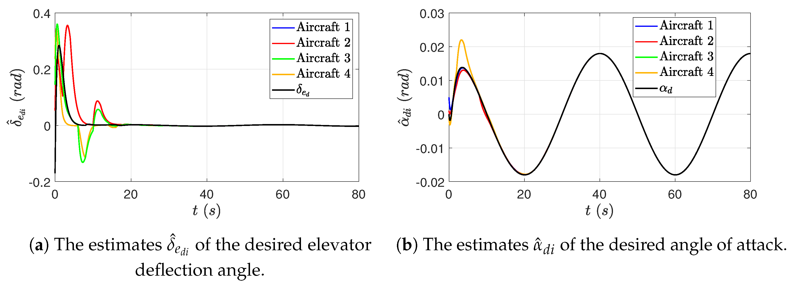
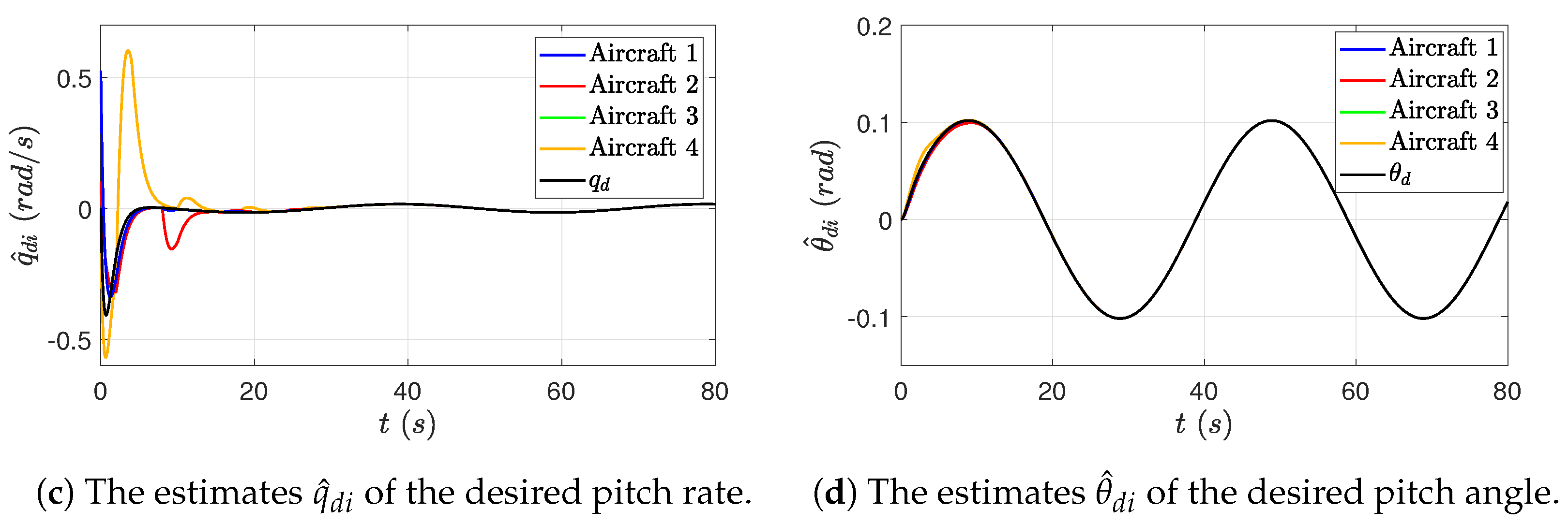
5.3.1. Simulation Results for Distributed Observer and Casual Stable Inversion

For all cases, we start with verifying the proposed Distributed Observer and Casual Stable Inversion.

As shown in Figure 4, the Distributed Observer of each aircraft generates asymptotic estimates of the states of the reference system (17) under a switching and occasionally disconnected communication topology. With these estimated reference system states, the Casual Stable Inversion is able to first calculate bounded estimates of the desired input $u_{di}$ and state ${\mathit{x}}_{di}$ in the new coordinate, and then use the inverse coordinate transformation (36) to generate the bounded estimates of the desired input ${\delta }_{e_{di}}$ and state ${\mathit{x}}_{o_{di}}$ in the original coordinate, as shown in Figure 5. These simulation results validate Lemmas 1–3, that is, the estimates of the desired input and states (the colored curves in Figure 5) converge asymptotically to the desired input and states generated by the reference system (the black curves in Figure 5), and thus, the estimation of reference signals is achieved by the proposed Distributed Observer and Casual Stable Inversion equipped on each aircraft.

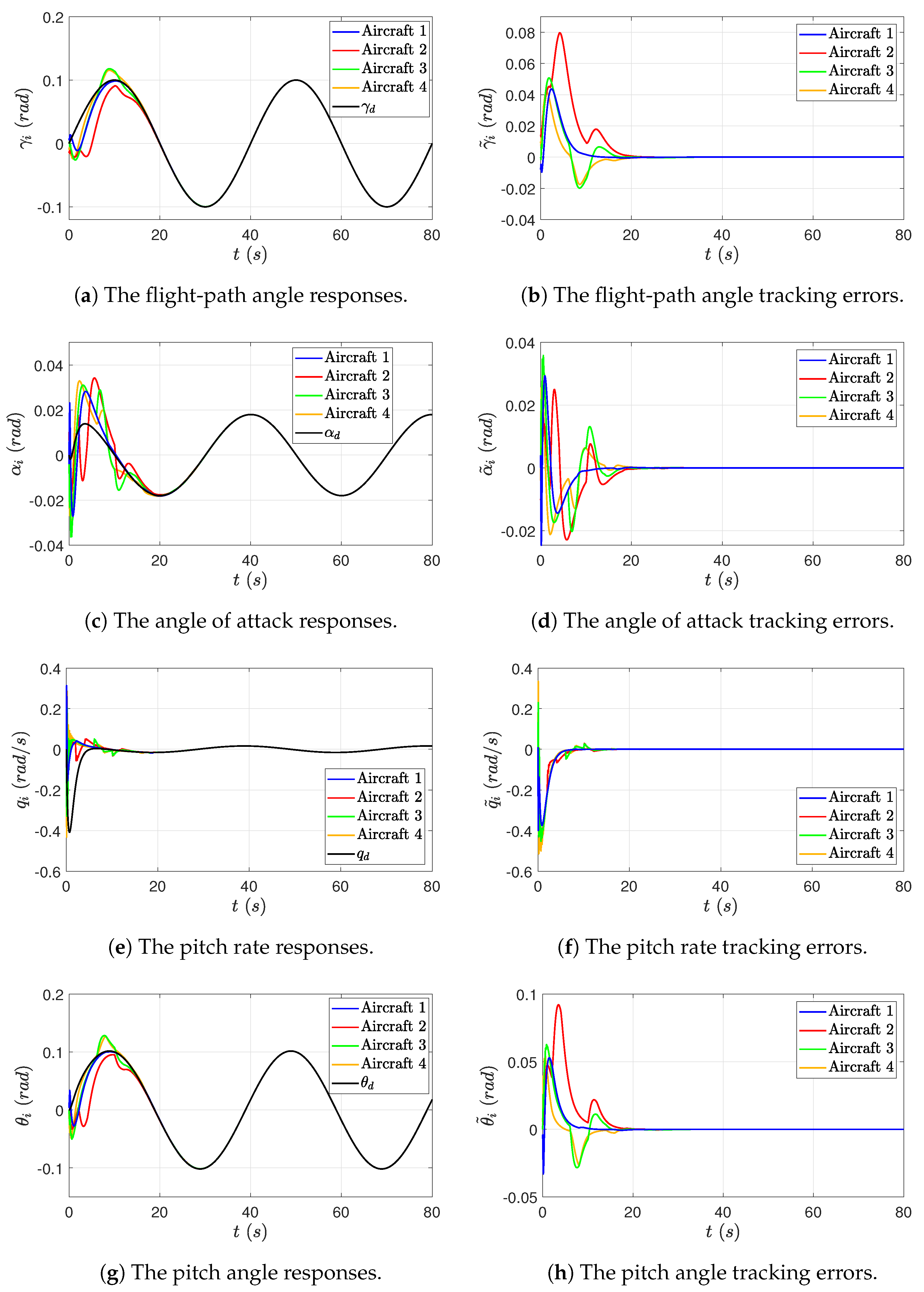
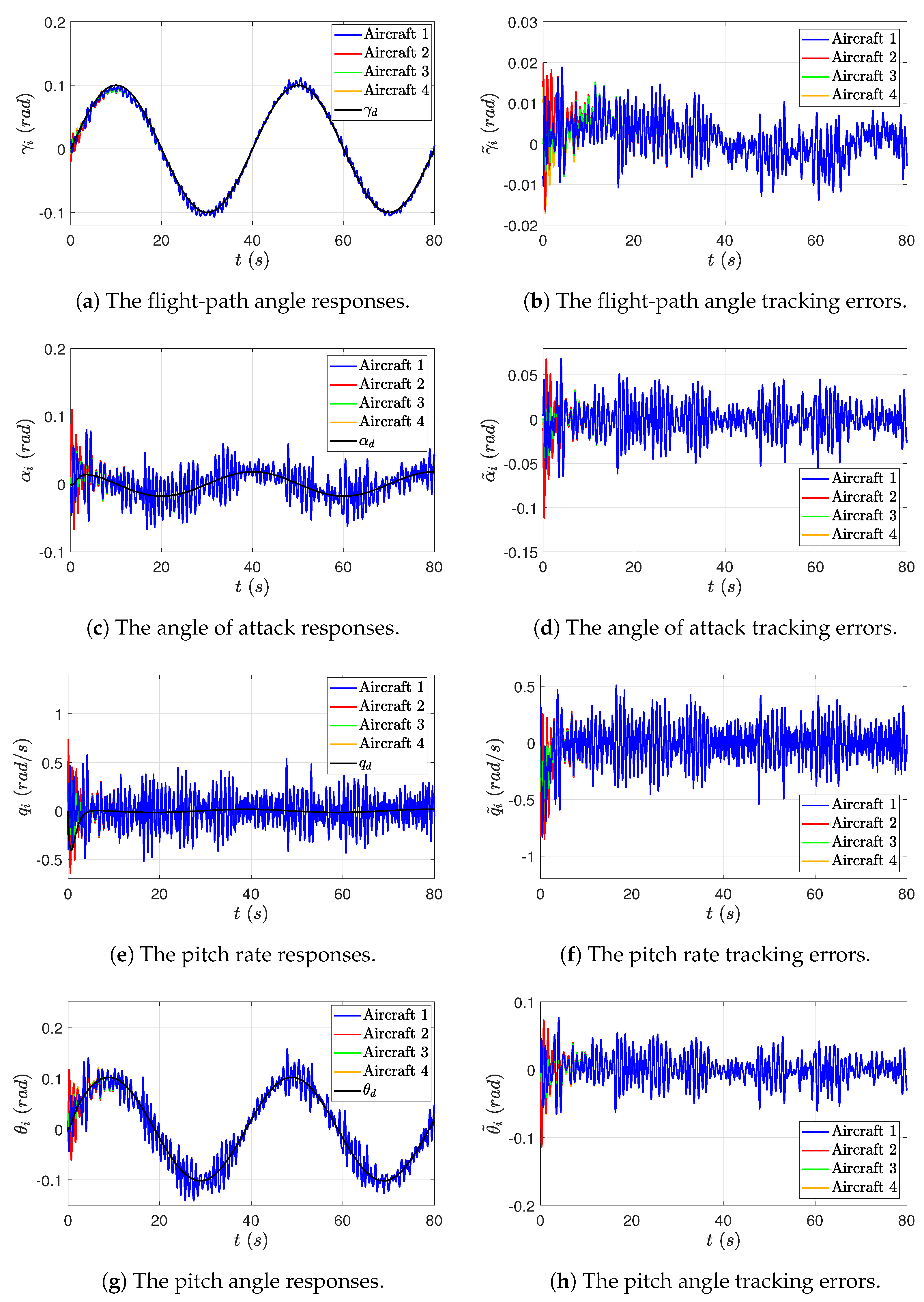
5.3.2. Simulation Results for Case 1

The state responses and tracking errors of each aircraft for Case 1 are shown in Figure 6 and Figure 7, from which it is seen that all the states are bounded, i.e., the objective (21) is achieved. Moreover, for the objectives (19) and (20), the proposed control delivers asymptotic tracking of the desired flight-path angle in the absence of measurement errors, and delivers approximate tracking with very small ultimate bounds ${\varsigma }_i=0.0014$ rad in the presence of measurement errors, thanks to the proposed Local Measurement Error Rejection Controller that actively estimates and compensates for the measurement errors.

It is also worth mentioning that the undershoot is observed in the flight-path angle responses, which results straightforwardly from the nature of non-minimum phase systems. The undershoot, by definition, is the phenomenon that the steady-state value of the system step response has a sign opposite from that of its first non-zero derivative at $t=0$ [35], or loosely speaking, that the system response initially starts off in the opposite direction of the expected steady-state value before moving towards the expected response. The undershoot occurs, according to [36], in systems with an odd number of real open right half-plane zeros, such as the flight-path angle control system of a conventional fixed-wing aircraft considered in this paper, which, in general, has one right half-plane zero. The physical reason behind this phenomenon lies in the coupling between the aerodynamic force and the corresponding pitch moment, which are simultaneously produced by the aircraft elevator. When the elevator deflection is positive, a downward force on the elevator makes the aircraft start with a height drop, and simultaneously a positive pitch moment is produced by this downward force, and then the nose of the aircraft rises. As the pitch angle and angle of attack increase, the aircraft gains additional lift to climb. The physics here matches well with the mathematical definition and description of the undershoot, since in the flight-path angle response, the derivative of the flight-path angle starts with a negative sign due to the downward force generated by the elevator. Therefore, during the control process, the flight-path angle response of each aircraft exhibits a “first goes down and then goes up” behavior.

Moreover, some sudden, dramatic state-trajectory changes are observed in Figure 6 and Figure 7, leading to the piece-wise continued smooth trajectories with several turning points. The fundamental reason behind these trajectories lies in the switching communication topology. The turning points in the red curves (Aircraft 2) at $t=10$ s are taken as an example herein, to show how the communication topology switching impacts the aircraft state responses and tracking errors. When $t=10$ s, the considered communication topology switches from Subgraph 1 to Subgraph 2, and Subgraph 2 is the only subgraph in the switching sequence that Aircraft 2 can obtain information from the aircraft formation (or more precisely speaking, Aircraft 2 has access to the reference system, but has no access to its neighbors). Under this circumstance, the Distributed Observer equipped on Aircraft 2 is enabled by the input information to actively synchronize its states with the reference system only during the period of time when the topology switches to Subgraph 2. During other time periods in the switching loop, Aircraft 2 does not receive any information from the aircraft formation, and thus, it is in a “self-control” mode. This explains why the states of the three modules of Aircraft 2 exhibit the sudden trajectory change behaviors at $t=10$ s. The same goes for other aircraft, i.e., the sudden trajectory changes in the blue, green, and orange curves.

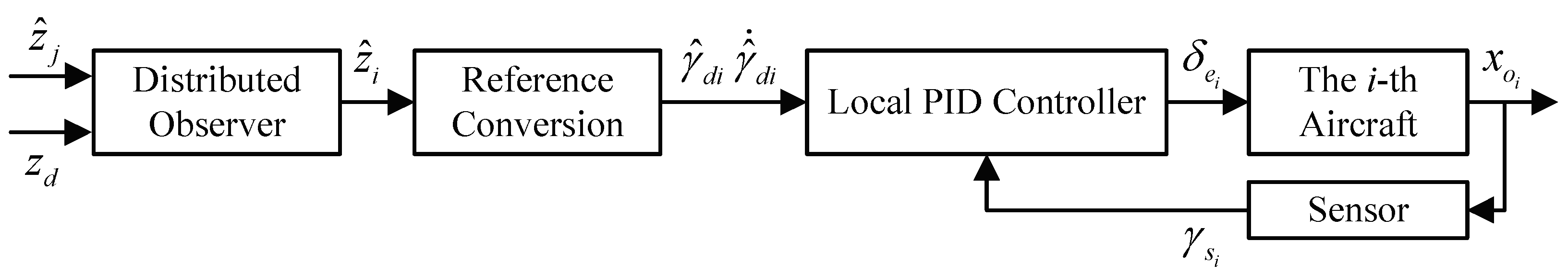
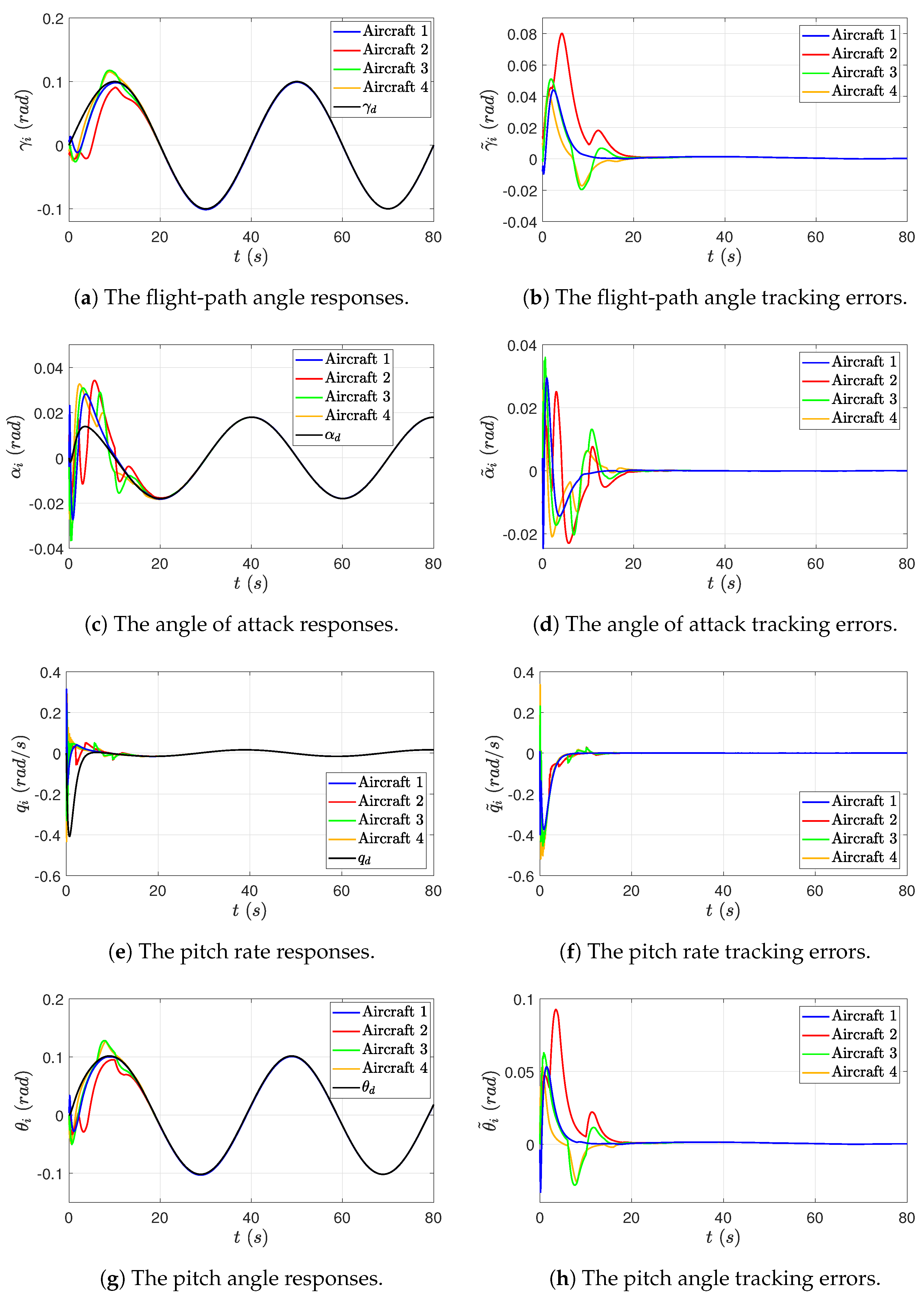
5.3.3. Simulation Results for Case 2

Figure 8 and Figure 9 demonstrate the simulation results for Case 2. It is observed that even in the absence of measurement errors, the state responses resulting from PID-based consensus control exhibit small residual tracking errors when tracking a time-varying flight-path angle reference, due to the fact that the PID controller (80) does not include the model-based feedforward control term. In addition, since the differentiator used in the PID controller (80) can add a dynamic delay to the estimate of ${\dot{\gamma }}_i$, which equivalently leads to an additional “measurement error” in the derivative feedback term, the resulting responses of flight-path angle and other system states include large oscillations. For unmanned fixed-wing aircraft, oscillations in flight-path angle, pitch angle, and angle of attack can endanger flight safety in practice, and thus, the PID-based consensus control may have certain limitations in transient performance. Furthermore, the PID controller lacks measurement error rejection mechanisms, and the derivative control term can further amplify the high-frequency measurement noises. Therefore, the trajectory tracking performance is greatly degraded in the presence of measurement errors.

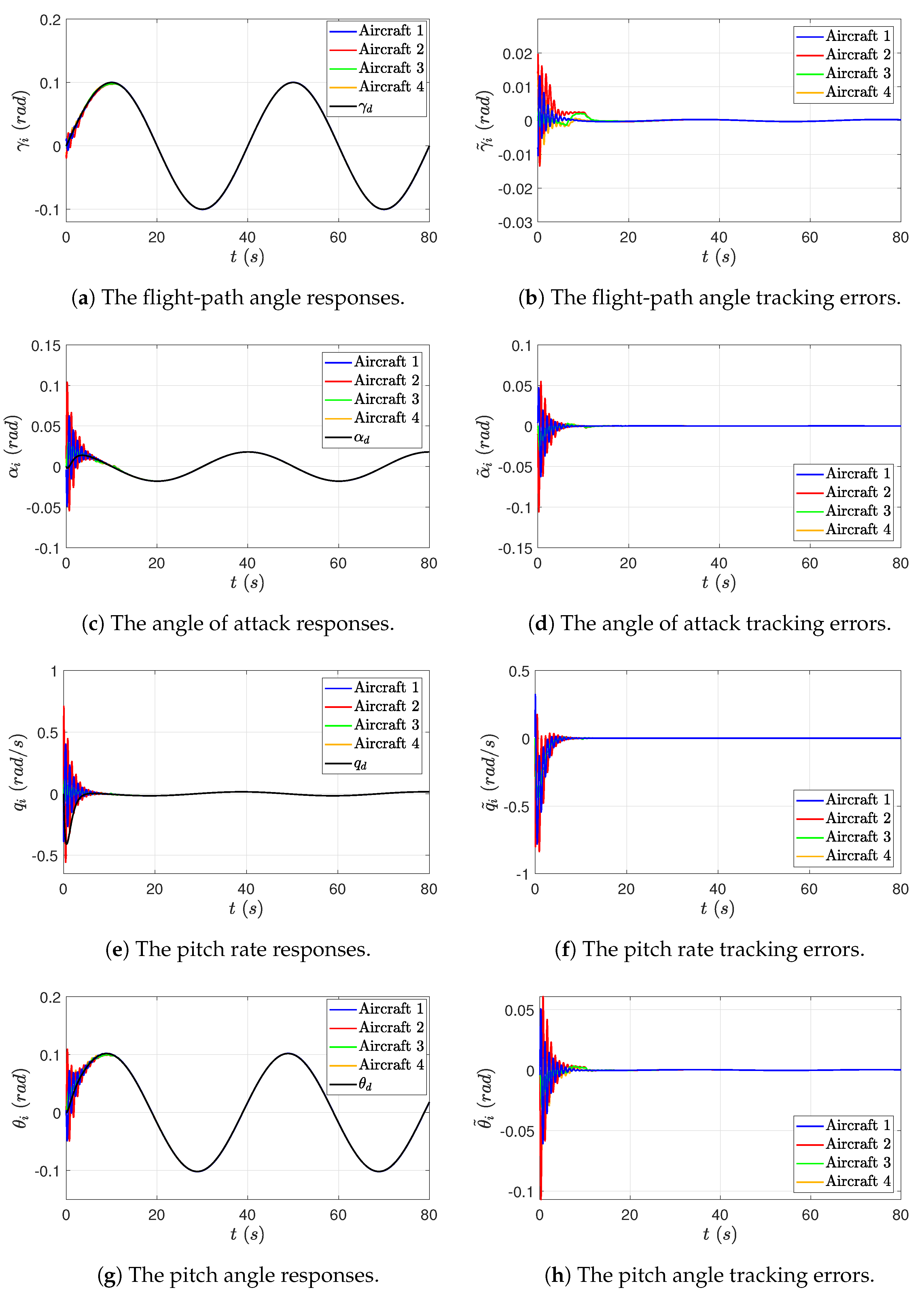
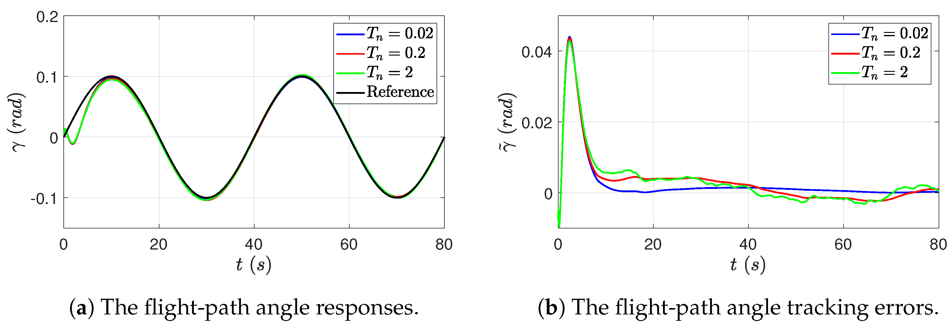
5.3.4. Simulation Results for Case 3

In Case 3, a set of MEE parameters $T_{ni}=\{0.02,0.2,2\}$ are applied to the Local Measurement Error Rejection Controller, and the simulation results are demonstrated in Figure 10. When $T_{ni}$ decreases, it is seen that not only the chattering, but also the ultimate bound of the flight-path angle tracking error is reduced. Thus, the tracking accuracy is improved. This result verifies Lemma 4 and Theorem 1.

6. Conclusions

This paper addresses the flight-path angle consensus tracking problem for a group of fixed-wing aircraft in the presence of measurement errors. The non-minimum phase properties of the flight-path angle dynamics are systematically taken into consideration in the control design to ensure the stability of the internal dynamics. A three-module control scheme is proposed, where a Distributed Observer is employed to provide the reference system estimation for the Casual Stable Inversion, which generates bounded estimates of the desired input and states for the Local Measurement Error Rejection Controller to achieve robust consensus control. The theoretical stability and performance analysis shows that the proposed control delivers asymptotic consensus tracking of the reference in the absence of measurement errors, and delivers approximate consensus tracking in the presence of measurement errors, within any specified ultimate bound if the MEE parameter $T_{ni}$ is appropriately selected. Simulation results in which the classic PID-based consensus control is compared are provided. The advantages of the proposed control are verified with respect to the transient oscillations and robustness against measurement errors. Besides, compared with most existing approaches (such as the aforementioned PID-based consensus control), which require multi-parameter tuning and optimization to enhance the control performance, the attractive feature of the proposed control is validated in the simulation, that is, the control performance regarding the steady-state tracking accuracy can be easily improved by reducing a single MEE parameter $T_{ni}$.

Future works include the extension of the proposed control scheme to: (i) heterogeneous aircraft formations; (ii) more sophisticated systems with possibly non-linear systems, switching dynamics in the presence of model uncertainties or unknown system parameters; and (iii) formations with antagonistic interactions.

References

1. Beard, R.W.; McLain, T.W.; Nelson, D.B.; Kingston, D.; Johanson, D. Decentralized Cooperative Aerial Surveillance using Fixed-Wing Miniature UAVs. Proc. IEEE 2006, 94, 1306–1324. [Google Scholar] [CrossRef]
2. Yu, Z.Q.; Zhang, Y.M.; Jiang, B.; Yu, X. Fault-Tolerant Time-Varying Elliptical Formation Control of Multiple Fixed-Wing UAVs for Cooperative Forest Fire Monitoring. J. Intell. Robot. Syst. 2021, 101, 48. [Google Scholar] [CrossRef]
3. Meng, W.; He, Z.R.; Su, R.; Yadav, P.K.; Teo, R.; Xie, L.H. Decentralized Multi-UAV Flight Autonomy for Moving Convoys Search and Track. IEEE Trans. Control Syst. Technol. 2016, 25, 1480–1487. [Google Scholar] [CrossRef]
4. Sun, Z.Y.; Garcia de Marina, H.; Anderson, B.D.; Yu, C.B. Collaborative Target-Tracking Control using Multiple Fixed-Wing Unmanned Aerial Vehicles with Constant Speeds. J. Guid. Control Dyn. 2021, 44, 238–250. [Google Scholar] [CrossRef]
5. Breakwell, J.V. Optimal Flight-Path-Angle Transitions in Minimum-Time Airplane Climbs. J. Aircr. 1977, 14, 782–786. [Google Scholar] [CrossRef]
6. de Lafontaine, J.; Lévesque, J.F.; Kron, A. Robust Guidance and Control Algorithms using Constant Flight Path Angle for Precision Landing on Mars. In Proceedings of the AIAA Guidance, Navigation, and Control Conference and Exhibit, Keystone, CO, USA, 21 August 2006; p. 6075. [Google Scholar]
7. Zhu, Y.; Zhu, B.; Qin, K.Y.; Liu, H.H.T. Distributed Control for Flight-Path Angle Synchronized Tracking of Multiple Fixed-Wing Aircraft. In Proceedings of the 2016 IEEE Chinese Guidance, Navigation and Control Conference (CGNCC), Nanjing, China, 12 August 2016; pp. 312–317. [Google Scholar]
8. Shi, L.; Cheng, Y.H.; Zhang, X.L.; Shao, J.L. Consensus Tracking Control of Discrete-Time Second-Order Agents over Switching Signed Digraphs with Arbitrary Antagonistic Relations. Int. J. Robust Nonlinear Control 2020, 30, 4826–4838. [Google Scholar] [CrossRef]
9. Ning, B.D.; Han, Q.L.; Zuo, Z.Y. Bipartite Consensus Tracking for Second-Order Multi-Agent Systems: A Time-Varying Function-Based Preset-Time Approach. IEEE Trans. Autom. Control 2020, 66, 2739–2745. [Google Scholar] [CrossRef]
10. Yoo, S.J.; Park, B.S. Connectivity-Preserving Approach for Distributed Adaptive Synchronized Tracking of Networked Uncertain Nonholonomic Mobile Robots. IEEE Trans. Cybern. 2017, 48, 2598–2608. [Google Scholar] [CrossRef]
11. Wang, C.L.; Wen, C.Y.; Wang, W.; Hu, Q.L. Output-Feedback Adaptive Consensus Tracking Control for A Class of High-Order Nonlinear Multi-Agent Systems. Int. J. Robust Nonlinear Control 2017, 27, 4931–4948. [Google Scholar] [CrossRef]
12. Ren, W. Consensus Tracking Under Directed Interaction Topologies: Algorithms and Experiments. IEEE Trans. Control Syst. Technol. 2010, 1, 230–237. [Google Scholar] [CrossRef]
13. Parivallal, A.; Sakthivel, R.; Wang, C. Guaranteed Cost Leaderless Consensus for Uncertain Markov Jumping Multi-Agent Systems. J. Exp. Theor. Artif. Intell. 2023, 35, 257–273. [Google Scholar] [CrossRef]
14. Zhang, X.Y.; Zhu, Z.H.; Liao, F.; Gao, H.; Li, W.H.; Li, G. Finite-Time Adaptive Consensus Tracking Control Based on Barrier Function and Cascaded High-Gain Observer. Drones 2023, 7, 197. [Google Scholar] [CrossRef]
15. Cao, W.J.; Liu, L.; Feng, G. Distributed Adaptive Output Consensus of Unknown Heterogeneous Non-Minimum Phase Multi-Agent Systems. IEEE/CAA J. Autom. Sin. 2023, 10, 997–1008. [Google Scholar] [CrossRef]
16. Meng, T.Y.; Xie, Y.J.; Lin, Z.L. Suboptimal Output Consensus of A Group of Discrete-Time Heterogeneous Linear Non-Minimum Phase Systems. Syst. Control Lett. 2022, 161, 105134. [Google Scholar] [CrossRef]
17. Shamsi, F.; Talebi, H.A.; Abdollahi, F. Output Consensus Control of Multi-Agent Systems with Nonlinear Non-Minimum Phase Dynamics. Int. J. Control 2018, 91, 785–796. [Google Scholar] [CrossRef]
18. Yang, H.; Jiang, B.; Zhang, H.G. Stabilization of Non-Minimum Phase Switched Nonlinear Systems with Application to Multi-Agent Systems. Syst. Control Lett. 2012, 61, 1023–1031. [Google Scholar] [CrossRef]
19. Lee, D. Robust Consensus of Linear Systems on Directed Graph with Non-Uniform Delay. IET Control Theory Appl. 2016, 10, 2574–2579. [Google Scholar] [CrossRef]
20. Shamsi, F.; Talebi, H.A.; Abdollahi, F. Output Consensus Control of Nonlinear Non-Minimum Phase Multi-Agent Systems Using Output Redefinition Method. AUT J. Model. Simul. 2017, 49, 3–12. [Google Scholar]
21. Li, W.H.; Zhu, Y.; Zhu, B.; Qin, K.Y.; Shi, M.J. Accurate Output Tracking Control for Nonminimum Phase Systems via An Iterative Redefinition-Based Method with Aircraft Application. In Proceedings of the 2022 34th Chinese Control and Decision Conference (CCDC), Hefei, China, 15 August 2022; pp. 4496–4502. [Google Scholar]
22. Chen, B.; Chu, B.; Geng, H. Distributed Iterative Learning Control for Constrained Consensus Tracking Problem. In Proceedings of the 2020 59th IEEE Conference on Decision and Control (CDC), Jeju, Republic of Korea, 14 December 2020; pp. 3745–3750. [Google Scholar]
23. Zhu, Y.; Chen, J.Y.; Zhu, B.; Qin, K.Y. Synchronised Trajectory Tracking for a Network of MIMO Non-Minimum Phase Systems with Application to Aircraft Control. IET Control Theory Appl. 2018, 12, 1543–1552. [Google Scholar] [CrossRef]
24. Kodhanda, A.; Kolhe, J.P.; Zeru, T.; Talole, S.E. Robust Aircraft Control Based on UDE Theory. Proc. Inst. Mech. Eng. Part G J. Aerosp. Eng. 2017, 231, 728–742. [Google Scholar] [CrossRef]
25. Kawamura, S.; Cai, K.; Kishida, M. Distributed Output Regulation of Heterogeneous Uncertain Linear Agents. Automatica 2020, 119, 109094. [Google Scholar] [CrossRef]
26. Zhang, M.R.; Saberi, A.; Stoorvogel, A.A. Synchronization for Heterogeneous Time-Varying Networks with Non-Introspective, Non-Minimum-Phase Agents in the Presence of External Disturbances with Known Frequencies. In Proceedings of the 2016 IEEE 55th Conference on Decision and Control (CDC), Las Vegas, NV, USA, 12 December 2016; pp. 5201–5206. [Google Scholar]
27. Shkolnikov, I.A. Output Tracking in Causal Nonminimum-Phase Nonlinear Systems in Sliding Modes. Ph.D. Dissertation, Department of Electrical and Computer Engineering, University of Alabama in Huntsville, Huntsville, AL, USA, 22 June 2003. [Google Scholar]
28. Su, Y.F.; Huang, J. Cooperative Output Regulation With Application to Multi-Agent Consensus Under Switching Network. IEEE Trans. Syst. Man Cybern. Part B Cybern. 2012, 42, 864–875. [Google Scholar]
29. Gopalswamy, S.; Hedrick, J.K. Tracking Nonlinear Non-Minimum Phase Systems using Sliding Control. Int. J. Control 1993, 57, 1141–1158. [Google Scholar] [CrossRef]
30. Devasia, S.; Chen, D.; Paden, B. Nonlinear Inversion-Based Output Tracking. IEEE Trans. Autom. Control 1996, 41, 930–942. [Google Scholar] [CrossRef]
31. Shtessel, Y.B.; Baev, S.; Edwards, C.; Spurgeon, S. HOSM Observer for a Class of Non-Minimum Phase Causal Nonlinear MIMO Systems. IEEE Trans. Autom. Control 2010, 55, 543–548. [Google Scholar] [CrossRef]
32. Zhu, Y.; Zhu, B.; Liu, H.H.T.; Qin, K.Y. A Model-Based Approach for Measurement Noise Estimation and Compensation in Feedback Control Systems. IEEE Trans. Instrum. Meas. 2020, 69, 8112–8127. [Google Scholar] [CrossRef]
33. Zhu, B.; Liu, H.H.T.; Li, Z. Robust Distributed Attitude Synchronization of Multiple Three-DOF Experimental Helicopters. IEEE Control Eng. Pract. 2015, 36, 87–99. [Google Scholar] [CrossRef]
34. Khalil, H.K.; Grizzle, J.W. Nonlinear Systems, 3rd ed.; Prentice-Hall: Upper Saddle River, NJ, USA, 2002; pp. 176–177. [Google Scholar]
35. Vidyasagar, M. On Undershoot and Nonminimum Phase Zeros. IEEE Trans. Autom. Control 1986, 31, 440. [Google Scholar] [CrossRef]
36. Delabarra, B.A. On Undershoot in SISO Systems. IEEE Trans. Autom. Control 1994, 39, 578–581. [Google Scholar]
Figure 1. The switching communication topology satisfying Assumption 4.
Drones 07 00350 g001
Figure 2. The proposed control scheme.
Drones 07 00350 g002
Figure 3. PID-based consensus control scheme.
Drones 07 00350 g003
Figure 4. Case 1, 2, and 3: The estimates and estimation error of the Distributed Observer under the time-varying communication topology 1.
Drones 07 00350 g004
Figure 5. Case 1, 2, and 3: The estimates of the desired input and states generated by the Casual Stable Inversion.
Drones 07 00350 g005aDrones 07 00350 g005b
Figure 6. Case 1: The proposed control in the absence of measurement errors: output/state responses and tracking errors.
Drones 07 00350 g006
Figure 7. Case 1: The proposed control in the presence of measurement errors: output/state responses and tracking errors.
Drones 07 00350 g007
Figure 8. Case 2: The PID-based consensus control in the absence of measurement errors: output/state responses and tracking errors.
Drones 07 00350 g008
Figure 9. Case 2: The PID-based consensus control in the presence of measurement errors: output/state responses and tracking errors.
Drones 07 00350 g009
Figure 10. Case 3: The proposed control in the presence of measurement errors under different T n i : output/state responses and tracking errors.
Drones 07 00350 g010