Autonomous Maneuver Decision-Making of UCAV with Incomplete Information in Human-Computer Gaming

Abstract

In human-computer gaming scenarios, the autonomous decision-making problem of an unmanned combat air vehicle (UCAV) is a complex sequential decision-making problem involving multiple decision-makers. In this paper, an autonomous maneuver decision-making method for UCAV that considers the partially observable states of Human (the adversary) is proposed, building on a game-theoretic approach. The maneuver decision-making process within the current time horizon is modeled as a game of Human and UCAV, which significantly reduces the computational complexity of the entire decision-making process. In each established game decision-making model, an improved maneuver library that contains all possible maneuvers (called the continuous maneuver library) is designed, and each of these maneuvers corresponds to a mixed strategy of the established game. In addition, the unobservable states of Human are predicted via the Nash equilibrium strategy of the previous decision-making stage. Finally, the effectiveness of the proposed method is verified by some adversarial experiments.

1. Introduction

With the advancement of science and technology, air combat equipment is accelerating innovation, which makes air combat showcase features such as high dynamics, strong confrontation, and incomplete information [1,2]. Traditionally, air combat commands have been performed by experienced pilots. However, an excellent pilot needs to gain combat experience from a lot of combat training, which requires huge costs. Moreover, limited by the physiology and mind of human pilots, it is difficult for human pilots to have a comprehensive grasp of the battlefield situation in the face of the new characteristics of modern air combat [3,4]. Therefore, it is particularly necessary to develop an autonomous decision-making system that can replace the role of human pilots [5,6]. Under this demand, the research on human-computer gaming has gradually emerged with the maturity of artificial intelligence technologies. As a human-computer gaming technology, the autonomous maneuver decision-making of an unmanned combat air vehicle (UCAV) versus human pilots has recently become a research hotspot [7,8].

In recent years, with the emergence of artificial intelligence technologies such as deep learning and reinforcement learning, the level of information acquisition, processing, and analysis of artificial intelligence-enabled machines has been greatly improved [9,10,11,12]. In the field of cognitive intelligence, human-computer gaming algorithms, represented by AlphaGo [13] and Libratus [14], have already defeated top human professional players in problems with defined boundaries and fixed rules. However, air combat decision-making is made in an open environment with no fixed rules and incomplete information [15,16,17]. In addition, air combat is different from scenarios such as Go and Texas Poker, which can be learned through multiple training sessions. As a result, existing human-computer gaming technologies cannot be migrated in parallel to air combat decision-making problems. In comparison, mathematical modeling of the human-computer gaming problem is a feasible research direction. Game theory, a mathematical tool used to describe the strategic interaction between multiple rational decision makers, has recently been used by many scholars to explore the decision-making approaches in air combat. In Ref. [18], a constraint strategy game approach was proposed to give intelligent decisions for multiple UCAVs with time-sensitive information. In Ref. [19], the task management and control problem was studied based on a dynamic game strategy, and a fast and optimal search algorithm inspired by graph theory and Kuhn–Munkres algorithm was designed to give the optimal decisions. In Ref. [20], a dimensionality reduction approach for matrix games was developed to provide efficient solutions for the multi-UCAV attack-defense decision-making problem.

As a typical air combat decision-making problem, maneuver decision-making has attracted a lot of interest from researchers in recent years [21,22,23]. A matrix game approach was proposed to generate maneuver decisions for low-flying aircraft during one-on-one air combat over hilly terrain in Ref. [24], which inspired the subsequent research of game theory in the maneuver decision-making problem. The maneuver library was designed, which consists of seven basic maneuvers. The maneuvers are max load factor turn left, max load factor turn right, max long acceleration, steady flight (flight with the current speed), max long deceleration, max load factor pull up, and max load factor push over. Then there are also some variants of the maneuver library, such as the maneuver library with 15 maneuvers [25], the maneuver library with 36 maneuvers [26], etc. An autonomous maneuver decision-making method was proposed in Ref. [27], based on an improved deep reinforcement learning (DRL) algorithm for a UCAV in short-range aerial combat. In the proposed algorithm, the final return value was incorporated into the previous steps, which overcomes the defects of traditional DRL in terms of training speed and convergence speed. A novel dynamic quality replay (DQR) method was proposed in Ref. [28] with the help of the DRL algorithm, which enables UAVs to effectively learn maneuver strategies from historical data without relying on traditional expert systems.

The above studies have gradually promoted the development of autonomous maneuver decision-making approaches. On this basis, we propose a maneuver decision-making method that considers the partially observable states of Human (the adversary) with a continuous maneuver decision-making library. We know that all existing maneuver libraries are composed of a limited number of basic maneuvers, so all available maneuvers designed in this way are discrete. However, in real maneuver decision-making process, all possible maneuvers are distributed in a continuous space. On this account, we design a continuous maneuver library that contains all possible maneuvers. In addition, the partially observable states of Human, as a class of incomplete information in air combat, is considered during the maneuver decision-making process. We know that maneuver decision-making is an iterative observation and decision-making process through interaction with the environment [29]. However, the current state of Human is sometimes unobservable in real air combat, due to equipment performance limitations and external disturbances. Considering this kind of incomplete information, we give a state prediction method when the state of Human is unobservable.

The main contributions of this paper are summarized as follows:

(1)

The maneuver decision-making process within the current time horizon is modeled as a game of UCAV and Human, which inherently reduces the computational complexity. In each established game decision-making model, a continuous maneuver library that contains all possible maneuvers is designed, where each maneuver corresponds to a mixed strategy of the game model, which not only enriches the maneuver library but also solves the problem of the executable of mixed strategies;

(2)

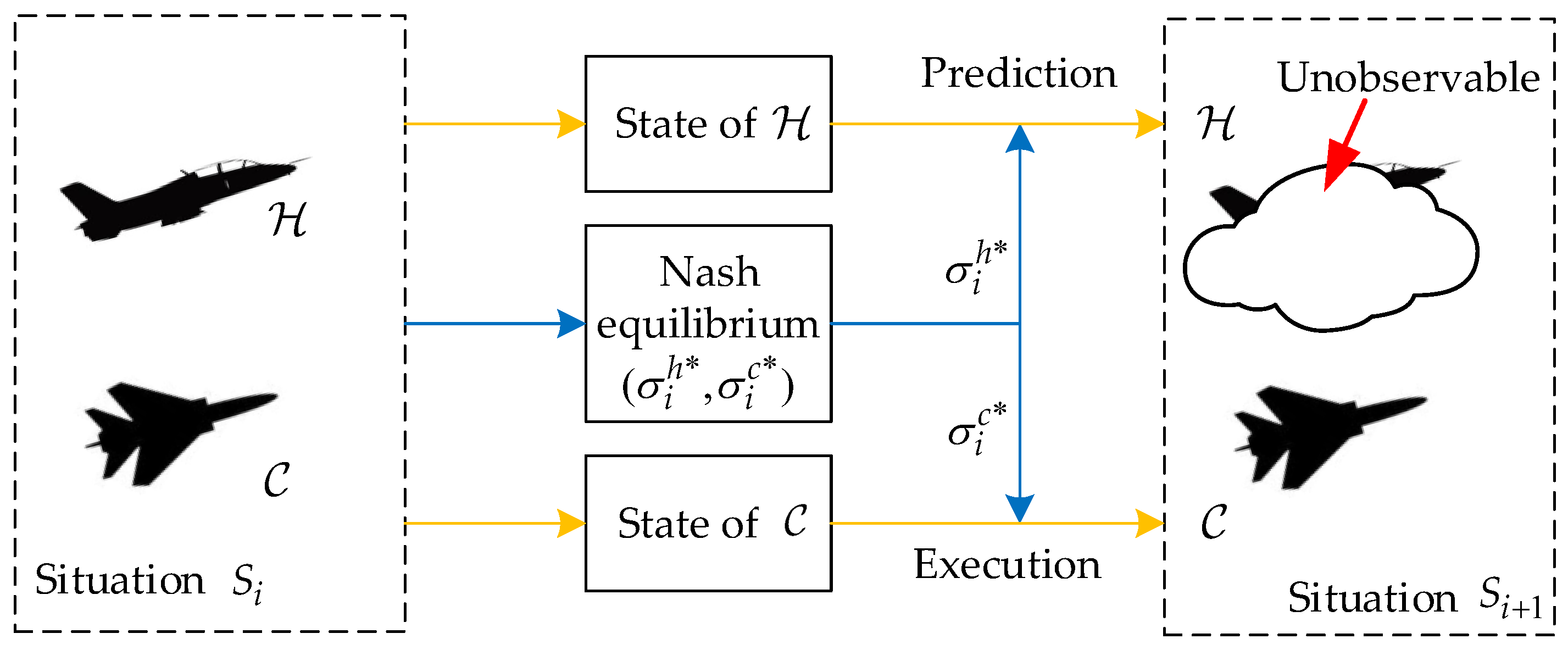
The partially observable state of Human is considered during the dynamic maneuver decision-making process of UCAV and Human, and a method to predict the unobservable state of Human is given via the Nash equilibrium strategy of the previous decision-making stage.

The structure of this paper is as follows. In Section 2, the maneuver decision-making problem in human-computer gaming is described, and a situation assessment method is reviewed to assess the quality of the maneuvers. In Section 3, an autonomous maneuver decision-making method is proposed for UCAV versus Human. Firstly, the decision-making process of the current time horizon is modeled as a game of both sides; then a continuous maneuver library that contains all possible maneuvers is designed; finally, a method for predicting the unobservable state of Human is given. In Section 4, simulations and analyses are presented to demonstrate the effectiveness of the proposed method.

2. Problem Formulation and Preliminaries

This paper considers the following maneuver decision-making problem in human-computer gaming scenarios: the two confronting entities in air combat, Human (the experienced pilot, labeled as $\mathcal{H}$) and Computer (the autonomous decision-making system of the UCAV, labeled as $\mathcal{C}$). Both aim to achieve the best possible attack position through a series of reasonable maneuvers. In this process, both $\mathcal{H}$ and $\mathcal{C}$ choose a maneuver according to the current air combat situation, then the current situation is changed to the next situation; after that, the two sides observe the current air combat situation and make further maneuver decisions, and so on, until one side occupies the best possible attack position and launches missiles. This is a sequential decision-making process involving two interacting decision-makers, which is essentially a dynamic game of $\mathcal{H}$ and $\mathcal{C}$.

We assume that both $\mathcal{H}$ and $\mathcal{C}$ complete a maneuver every time $\Delta t$. As a consequence, the maneuver decision-making process of $\mathcal{H}$ and $\mathcal{C}$ can be divided into multiple consecutive decision-making stages, as shown in Figure 1, where $t_i$ ($i=1,2,\cdots ,T-1$) is the i-th decision point, satisfying $t_{i+1}-t_i=\Delta t$, $t_T$, which is an ideal attack position of one side, $S_i$ is the air combat situation of $\mathcal{H}$ and $\mathcal{C}$ at time $t_i$, $a_i^h$ and $a_i^c$ represent the maneuvers taken by $\mathcal{H}$ and $\mathcal{C}$ at time $t_i$, respectively.

During the maneuver decision-making process of $\mathcal{H}$ and $\mathcal{C}$, $\mathcal{C}$ first receives the air combat information of both sides in real time through airborne sensors and ground base stations, and then conducts a situational assessment based on the received information, which is the basis for subsequent maneuver decision-making. The air combat situation of $\mathcal{H}$ and $\mathcal{C}$ is given in Figure 2, where $R^{hc}$ is the distance between $\mathcal{H}$ and $\mathcal{C}$, $H^{hc}$ is the height difference between them, $\phi$ and q are the target azimuth and target entry angle of $\mathcal{C}$ with respect to $\mathcal{H}$, respectively, $V^h$ and $V^c$ are the speeds of $\mathcal{H}$ and $\mathcal{C}$, respectively. We point out that the above parameters can be calculated from the position and speed of $\mathcal{H}$ and $\mathcal{C}$. Thus, the states of $\mathcal{H}$ and $\mathcal{C}$ are defined as their positions and speeds, and are denoted as $S_i^h$ and $S_i^c$, respectively.

The situation assessment index system is composed of speed advantage, angle advantage, distance advantage, height advantage, and performance advantage. In Ref. [30], the speed advantage function considers the speed of both aircrafts. On this basis, we propose an improved speed advantage function which considers both the speed of the aircrafts and the speed of the missiles. The speed advantage function $W_v$ is given as follows:

$$\begin{array}{c}\hfill W_v={\lambda }_1{W}_{v,a}+{\lambda }_2{W}_{v,m},\end{array}$$

(1)

where $W_{v,a}$ is the aircraft speed advantage function, $W_{v,m}$ is the missile speed advantage function, and ${\lambda }_1$ and ${\lambda }_2$ are weight coefficients (satisfying ${\lambda }_1,{\lambda }_2\ge 0$, ${\lambda }_1+{\lambda }_2=1$). For the aircraft speed advantage function $W_{v,a}$, please refer to Ref. [30]. Similar to $W_{v,a}$, we give the missile speed advantage function $W_{v,m}$ as follows:

$$\begin{array}{c}\hfill W_{v,m}=\left\{\begin{array}{cc}0.1\hfill & V_{mi}^c\le 0.6V_{mi}^h,\hfill \\ -0.5+V_{mi}^c/V_{mi}^h\hfill & 0.6V_{mi}^h<V_{mi}^c<1.5V_{mi}^h,\hfill \\ 1\hfill & V_{mi}^c\ge 1.5V_{mi}^h,\hfill \end{array}\right.\end{array}$$

(2)

where $V_{mi}^c$ and $V_{mi}^h$ are the missile speeds of $\mathcal{C}$ and $\mathcal{H}$ respectively.

For detailed formulas of angle advantage, distance advantage, height advantage, and performance advantage, please see Refs. [3,30,31,32]. By combining the advantage functions of speed, angle, distance, height, and performance, the overall situation advantage of $\mathcal{C}$ over $\mathcal{H}$ can finally be obtained [3].

3. Design of the Maneuver Decision-Making Method

In this section, an autonomous maneuver decision-making method for $\mathcal{C}$ that considers the partially observable states of $\mathcal{H}$ is proposed. The maneuver decision-making process within the current time horizon is modeled as a game of $\mathcal{H}$ and $\mathcal{C}$. In each game, a continuous maneuver library that contains all possible maneuvers is designed. Finally, a method to predict the unobservable state of $\mathcal{H}$ is proposed. The overall flow of the proposed autonomous maneuver decision-making method is given in Figure 3, where the game decision-making model of $\mathcal{C}$ and $\mathcal{H}$ at the i-th decision-making stage is constructed based on the continuous maneuver library and situation assessment method; then the strategy $s^{c*}$ executed by $\mathcal{C}$ is obtained through the calculated Nash equilibrium $(s_i^{h*},s_i^{c*})$ of the established game; subsequently, observe the state of $\mathcal{H}$ when this state is observable, otherwise, the unobservable state of $\mathcal{H}$ is predicted via the Nash equilibrium strategy $s^{h*}$; if one side reaches a suitable attack position, launch the guns/missiles, otherwise update the air combat situation and repeat the above maneuver decision-making process.

3.1. Game Decision-Making Model of the Current Time Horizon

As a dynamic game process, the decision time of maneuver decision-making increases exponentially with the increase of the decision stages. As a consequence, it is unrealistic to consider the entire maneuver decision-making process at once. Here, we borrow the ideal of moving horizon solutions of dynamic games in Ref. [33], and the maneuver decision-making process within the current time horizon is modeled as a game of $\mathcal{H}$ and $\mathcal{C}$. That is, we do not consider the entire decision-making process at once, but limit the computation to a short time horizon that may involve only the next few decision-making stage, which can significantly reduce the computational complexity. Formally, the i-th decision stage of the maneuver decision-making process is modeled as the following game: $G_i=\langle S_i,A^h,A^c,u^h,u^c\rangle$, where

• $S_i$ is the air combat situation of the i-th decision-making stage;
• $A^h$ and $A^c$ are the maneuver sets of $\mathcal{H}$ and $\mathcal{C}$, respectively. Since both $\mathcal{H}$ and $\mathcal{C}$ have full maneuverability, we assume that they have the same maneuver set, i.e., $A^h=A^c$;
• $u_i^c:A^h\times A^c\to \mathbb{R}$ is the payoff function of $\mathcal{C}$, which associates each $(a_i^h,a_i^c)\in A^h\times A^c$ with a real value $u_i^c(a_i^h,a_i^c)$. The payoff function $u_i^h$ of $\mathcal{H}$ is defined as $u_i^h=-u_i^c$, due to the adversarial nature of $\mathcal{H}$ and $\mathcal{C}$.

Below we give the construction of the payoff functions. The purpose of $\mathcal{H}$ or $\mathcal{C}$ in making maneuver decisions is to have a situational advantage over the other side. Therefore, the payoff function is defined as the added value of the situation assessment after taking a certain maneuver combination. Formally, the payoff function $u_i^c$ of $\mathcal{C}$ is constructed as follows:

$$\begin{array}{c}\hfill u_i^c(a_i^h,a_i^c)=W\left(S_{i+1}\right)-W\left(S_i\right),\end{array}$$

(3)

where $S_{i+1}$ is the air combat situation after taking the maneuvers $a_i^h$ and $a_i^c$, $W\left(S_{i+1}\right)$ and $W\left(S_i\right)$ are the situation assessment values of $\mathcal{C}$ under the air combat situations $S_{i+1}$ and $S_i$, respectively.

In the context of game theory, $A^h$ and $A^c$ are called the pure strategy sets of $\mathcal{H}$ and $\mathcal{C}$, respectively. However, the strategy chosen in a game is often a probability distribution over the set of a pure strategy set, which is called a mixed strategy. Formally, a mixed strategy of $\mathcal{H}$ is a probability distribution ${\sigma }_i^h:A^h\to [0,1]$, which associates a pure strategy $a_i^h\in A^h$ with a value ${\sigma }_i^h\left(a_i^h\right)$, where ${\sigma }_i^h\left(a_i^h\right)$ represents the probability of choosing strategy $a_i^h$. A pure strategy is usually a finite set, so a mixed strategy ${\sigma }_i^h$ can be represented by the range of the probability distribution (a probability vector). The set of all probability distributions on $A^h$ is called the mixed strategy set of $\mathcal{H}$, denoted as $\Delta \left(A^h\right)$. Similarly, the mixed strategy set of $\mathcal{C}$ is given as $\Delta \left(A^c\right)$. The mixed strategy is essentially an expansion of the pure strategy. Naturally, the payoff function $U_i^c$ of $\mathcal{C}$ defined on the mixed strategy set can be given as [34]:

$$\begin{array}{c}\hfill U_i^c({\sigma }_i^h,{\sigma }_i^c)=\sum _{a_i^h\in A^h}\sum _{a_i^c\in A^c}{\sigma }_i^h\left(a_i^h\right)·{\sigma }_i^c\left(a_i^c\right)·u_i^c(a_i^h,a_i^c),\end{array}$$

(4)

where ${\sigma }_i^h\in \Delta \left(A^h\right)$, ${\sigma }_i^c\in \Delta \left(A^c\right)$. In fact, $U_i^c({\sigma }_i^h,{\sigma }_i^c)$ is the expected payoff of $\mathcal{C}$ on the probability distribution combination $({\sigma }_i^h,{\sigma }_i^c)$.

Nash equilibrium is a widely adopted solution concept of a game. In a Nash equilibrium, no player can increase his own payoff by unilaterally changing his current strategy. For the above game $G_i=\langle S_i,A^h,A^c,U^h,U^c\rangle$, a strategy combination $(a_i^{h*},a_i^{c*})\in A^h\times A^c$ is called a pure strategy Nash equilibrium of G, if for each $a_i^h\in A^h$, and each $a_i^c\in A^c$, the following inequalities hold [34]:

$$\begin{array}{c}\hfill u_i^c(a_i^{h*},a_i^c)\le u_i^c(a_i^{h*},a_i^{c*})\le u_i^c(a_i^h,a_i^{c*}).\end{array}$$

(5)

Similarly, a strategy combination $({\sigma }_i^{h*},{\sigma }_i^{c*})\in \Delta \left(A^h\right)\times \Delta \left(A^c\right)$ is called a mixed strategy Nash equilibrium of G, if for each ${\sigma }_i^h\in \Delta \left(A^h\right)$, and each ${\sigma }_i^c\in \Delta \left(A^c\right)$, there is [34]

$$\begin{array}{c}\hfill U_i^c({\sigma }_i^{h*},{\sigma }_i^c)\le U_i^c({\sigma }_i^{h*},{\sigma }_i^{c*})\le U_i^c({\sigma }_i^h,{\sigma }_i^{c*}).\end{array}$$

(6)

It has been proved by John Nash that every game has at least one mixed strategy Nash equilibrium [34]. However, not all games have a pure strategy Nash equilibrium. A mixed strategy Nash equilibrium of a two-player zero-sum game can be obtained by the following lemma.

Lemma 1

(Parthasarathy and Raghavan [35]). Consider a two-player zero-sum game $G=\langle A^h,A^c,B\rangle$, where $A^h$ and $A^c$ are the strategy sets of players $\mathcal{H}$ and $\mathcal{C}$, respectively, $B={\left(b_{ij}\right)}_{n\times m}$ is the payoff matrix of $\mathcal{C}$. If $\overline{x}=({\overline{x}}_1,{\overline{x}}_2,\cdots ,{\overline{x}}_n)$ and $\overline{y}=({\overline{y}}_1,{\overline{y}}_2,\cdots ,{\overline{y}}_m)$ are the optimal solutions of the following dual linear programming (7) and (8), respectively, then $(x^{*},y^{*})$ is a Nash equilibrium of G, where $x^{*}=v\overline{x}$, $y^{*}=v\overline{y}$, $v={\left({\sum }_{i=1}^n{\overline{x}}_i\right)}^{-1}$.

$$\left\{\begin{array}{cc}\hfill \min & \sum _{i=1}^n{x}_i\hfill \\ \hfill \mathrm{s}.\mathrm{t}.& \sum _{i=1}^n{x}_i{b}_{ij}\ge 1,j=1,2,\cdots ,m\hfill \\ \hfill & x_i\ge 0,i=1,2,\cdots ,n\hfill \end{array}\right.$$

(7)

$$\left\{\begin{array}{cc}\hfill \max & \sum _{j=1}^m{y}_j\hfill \\ \hfill \mathrm{s}.\mathrm{t}.& \sum _{j=1}^m{y}_j{b}_{ij}\le 1,i=1,2,\cdots ,n\hfill \\ \hfill & y_j\ge 0,j=1,2,\cdots ,m.\hfill \end{array}\right.$$

(8)

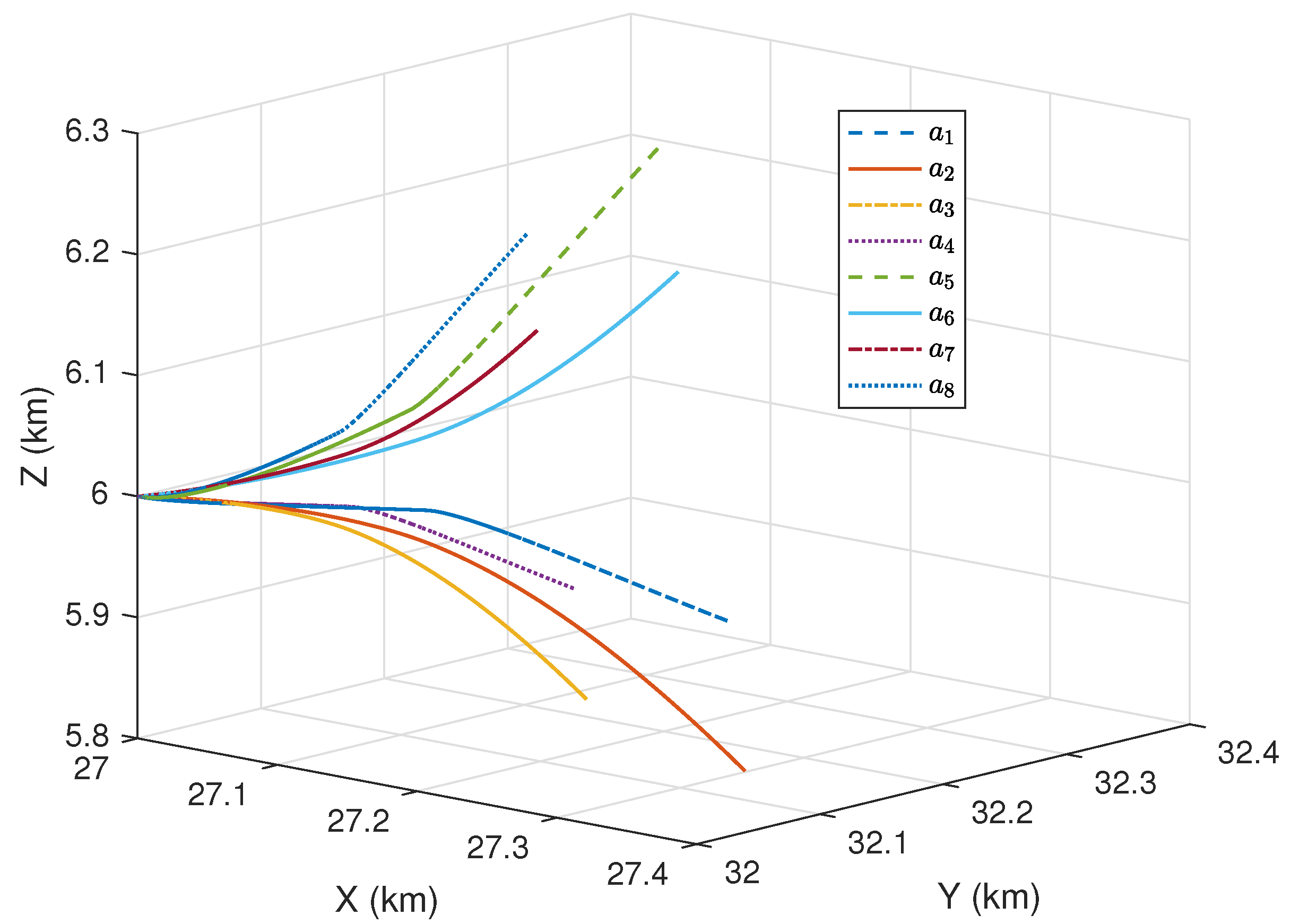
3.2. Continuous Maneuver Library

In this section, the maneuver library is designed. We know that the Nash equilibrium of a game is selected from the mixed strategy set, so the mixed strategy set is actually the maneuver library (the set of all possible maneuvers). In other words, the mixed strategy set $\Delta \left(A^h\right)$ ($\Delta \left(A^c\right)$) corresponds to the maneuver library. In order to design the maneuver libraries $\Delta \left(A^h\right)$ and $\Delta \left(A^c\right)$, it is only necessary to design the pure policy sets $A^h$ and $A^c$ (called the maneuver sets).

Before designing the maneuver sets $A^h$ and $A^c$, we first investigate all the possible maneuvers of $\mathcal{H}$ and $\mathcal{C}$. For a maneuver of $\mathcal{H}$ or $\mathcal{C}$, its control variables are decomposed into the following three parts: horizontal control variable, vertical control variable, and acceleration control variable, which are denoted as $c_h$, $c_v$, and $c_a$, respectively. So a maneuver $a^h\in A^h$ (or $a^c\in A^c$) can be represented by a three-dimensional vector as follows: $a^h=(c_h,c_v,c_a)$. For the three variables we give the following design:

• The horizontal control variable $c_h$ belongs to the interval $[-1,1]$, where $c_h=-1$ represents max load factor turn left, $c_h=1$ represents max load factor turn right, $a_h=0$ represents no horizontal turning maneuver, $c_h\in (-1,0)$ represents $c_h$ times max load factor turn left, and $c_h\in (0,1)$ represents $c_h$ times max load factor turn right;
• The vertical control variable $c_v$ belongs to $[-1,1]$, where $c_v=-1$ represents max load factor push over, $c_v=1$ represents max load factor pull up, $c_v=0$ represents no vertically turning maneuvers, $c_v\in (-1,0)$ represents $c_v$ times max load factor push over, and $c_v\in (0,1)$ represents $c_v$ times max load factor pull up;
• The acceleration control variable $c_a$ belongs to $[-1,1]$, where $c_a=-1$ represents the maximum thrust deceleration, $c_a=1$ represents the maximum thrust acceleration, $c_a=0$ represents that the thrust is 0, $c_a\in (-1,0)$ represents $c_a$ times maximum thrust deceleration, and $c_a\in (0,1)$ represents $c_a$ times maximum thrust acceleration.

As a result, all possible maneuvers form the cube ${[-1,1]}^3$ in three-dimensional space, as shown in Figure 4.

Now, we construct $A^h$ as the set of all the vertices of the cube, in other words,

$$\begin{array}{c}\hfill A^h:=\{a_1,a_2,\cdots ,a_8\}.\end{array}$$

The vertices $a_1,a_2,\cdots ,a_8$ are marked in Figure 4, where

$$\begin{array}{cc}{a}_1=(-1,-1,1),\hfill & a_2=(1,-1,1),\hfill \\ a_3=(1,-1,-1),\hfill & a_4=(-1,-1,-1),\hfill \\ a_5=(-1,1,1),\hfill & a_6=(1,1,1),\hfill \\ a_7=(1,1,-1),\hfill & a_8=(-1,1,-1).\hfill \end{array}$$

Since $A^h=A^c$, the set $A^c$ is also given as

$$\begin{array}{c}\hfill A^c:=\{a_1,a_2,\cdots ,a_8\}.\end{array}$$

Below we explain the advantages of defining the pure strategy sets in this way. As we discussed above, the Nash equilibrium of a game is often in the form of a mixed strategy. If the pure strategy set is defined as the vertices of the cube, i.e., a point in three-dimensional space, then a mixed strategy is a convex combination of these vertices, which is a point inside the cube. Note that each point in the cube corresponds to a maneuver that can be executed, so each mixed strategy is an executable maneuver. More precisely, a mixed strategy ${\sigma }_i^h$ of $\mathcal{H}$ can be represented by the following point inside the cube:

$$\begin{array}{c}\hfill \sum _{k=1}^8{\sigma }_i^h\left(a_k\right)·a_k,\end{array}$$

(9)

where ${\sigma }_i^h\left(a_k\right)$ is the probability of executing the pure strategy $a_k$ in the mixed strategy. Furthermore, the set of all mixed strategies constitutes the whole cube, that is, the mixed strategy set $\Delta \left(A^h\right)$ can be represented by the cube ${[-1,1]}^3$. Compared with the existing discrete maneuver library, the maneuver library $\Delta \left(A^h\right)$ we designed is called the continuous maneuver library.

Remark 1.

We know that although the concept of mixed strategy is widely used, it has also been controversial since it was proposed. This is because it implements specific strategies in a probabilistic manner. Significantly, constructing the pure strategy set in this way not only solves the defect that the mixed strategy is not easy to implement, but also expands the maneuver library to include all possible maneuvers.

3.3. Prediction of the Unobservable State of Human

As we designed above, our maneuver decision-making method is an observation-decision-execution cycle. However, due to the uncertainty and various disturbances in the air combat process, not all the states of $\mathcal{H}$ can be completely observed in the whole decision-making stages. When the state of $\mathcal{H}$ is unobservable, it is difficult to make the subsequent decision-making. To this end, we give a method to predict the state of $\mathcal{H}$ based on the Nash equilibrium calculated in the previous decision-making stage.

The prediction method we propose is based on the following idea: as a rational decision maker, $\mathcal{H}$ is considered to take an optimal action (the Nash equilibrium strategy) at time $t-1$, so the state after taking this action can be viewed as its predicted state at time t. Essentially, the proposed state prediction method is an intention prediction method.

In fact, regardless of whether the state of $\mathcal{H}$ is observable at time $t+1$, we have established the game model $G_i=\langle S_i,A^h,A^c,u^h,u^c\rangle$ of $\mathcal{H}$ and $\mathcal{C}$ at situation $S_i$, furthermore, the Nash equilibrium of G is calculated as $({\sigma }_i^{h*},{\sigma }_i^{c*})$, where ${\sigma }_i^{c*}$ is the maneuver that $\mathcal{C}$ needs to perform at the i-th decision-making stage. At time $t+1$, if the state of $\mathcal{H}$ is observable, the observed state of $\mathcal{H}$ and the state of $\mathcal{C}$ constitute the new air combat situation $S_{i+1}$, and the decision-making of next stage is continued; if the state of $\mathcal{H}$ is unobservable, the Nash equilibrium strategy of the previous step ${\sigma }_i^{h*}$ is used to predict the state of $\mathcal{H}$. This is because as a rational decision maker, the optimal maneuver of $\mathcal{H}$ is the Nash equilibrium strategy. As a result, ${\sigma }_i^{h*}$ is taken as the predicted action of the previous step, and the state under ${\sigma }_i^{h*}$ is taken as the predicted state of $\mathcal{H}$. The above method of predicting the state of $\mathcal{H}$ is shown in Figure 5, which is called the Nash equilibrium based state prediction (NESP) algorithm, and the detailed steps to predict the state of $\mathcal{H}$ at time $t_{i+1}$ by NESP algorithm are given as follows:

Step 1. Establish the game decision-making model $G_i=\langle S_i,A^h,A^c,u^h,u^c\rangle$ under the situation $S_i$;

Step 2. Calculate the Nash equilibrium $({\sigma }_i^{h*},{\sigma }_i^{c*})$ of G;

Step 3. The maneuver strategy ${\sigma }_i^{h*}$ is considered to be the strategy adopted by $\mathcal{H}$ at the i-th decision-making stage;

Step 4. Calculate the state $S_{i+1}^h$ of $\mathcal{H}$ after taking maneuver strategy ${\sigma }_i^{h*}$ according to the dynamical model [36], that is, the position and speed of $\mathcal{H}$ at time $t_{i+1}$.

Remark 2.

The above state prediction method is effective when the state of the adversary is unobservable in a short time (small continuous steps). However, when multiple continuous states of the adversary are unobservable, the reliability of the predicted results cannot be guaranteed. This is because in this case it is necessary to continue to predict the state of the next step based on the predicted state of the previous step. As a consequence, the deviations in the predicted results will accumulate as the number of predicted steps increases. Fortunately, what is faced in real air combat is more of this kind of unobservability in small steps.

To sum up, an automatic maneuver decision-making method that considers the partially observable states of $\mathcal{H}$ and a continuous maneuver library is designed, which is summarized as the automatic maneuver decision-making algorithm (AMDM) in Algorithm 1.

Algorithm 1: Automatic maneuver decision-making algorithm (AMDM)

Input: Initial air combat situation of $\mathcal{H}$ and $\mathcal{C}$: $S_1$;

Output: The maneuver decision sequence of $\mathcal{C}$: ${\sigma }_1^{c*}$, ${\sigma }_2^{c*}$, ⋯, ${\sigma }_T^{c*}$

1 Initialize$i=1$; 2 whileBoth$\mathcal{H}$and$\mathcal{C}$do not reach the ideal attack position in situation$S_i$do

13 Launch missiles 14 return${\sigma }_1^{c*}$, ${\sigma }_2^{c*}$, ⋯, ${\sigma }_T^{c*}$;

4. Simulations

In Section 4, numerical simulations and analyses of the proposed method are presented. First, an example of one decision-making stage in air combat is given to illustrate the computational flow of the proposed method; then, some comparative experiments are carried out, and the simulation analyses are given to illustrate the effectiveness of our method.

4.1. A Numerical Example of Maneuver Decision-Making in One Decision-Making Phase

Consider the maneuver decision scenario of $\mathcal{H}$ and $\mathcal{C}$, and their initial parameters, which are given in

Table 1. Initial parameters of $\mathcal{H}$ and $\mathcal{C}$ in a numerical example.

Symbol	Description	$\mathcal{H}$	$\mathcal{C}$
$P_x\left(\mathrm{km}\right)$	X coordinate of position	81	27
$P_y\left(\mathrm{km}\right)$	Y coordinate of position	70	32
$P_z\left(\mathrm{km}\right)$	Z coordinate of position	7	6
$V_x(\mathrm{km}·{\mathrm{h}}^{-1})$	X coordinate of speed	$-425$	234
$V_y(\mathrm{km}·{\mathrm{h}}^{-1})$	Y coordinate of speed	$-252$	215
$V_z(\mathrm{km}·{\mathrm{h}}^{-1})$	Z coordinate of speed	$-23$	32
$D_{mi}\left(\mathrm{km}\right)$	Maximum missile launch distance	54	46
$D_{ra}\left(\mathrm{km}\right)$	Maximum radar detection distance	139	127
$V_{mi}\left(\mathrm{Ma}\right)$	Maximum missile speed	$4.1$	$3.8$
$N_{mi}$	Number of carried missiles	2	3

. As discussed in Section 3.2, the maneuver set $A^h$ of $\mathcal{H}$ (the maneuver set $A^c$ of $\mathcal{C}$) is composed of the following eight maneuvers: $a_1,a_2,\cdots ,a_8$, where $a_k$ is a three-dimensional vector representing a specific maneuver of $\mathcal{H}$ or $\mathcal{C}$. Under the initial states, the trajectories of $\mathcal{C}$ are shown in Figure 6 when it chooses these eight maneuvers, and the trajectory of $\mathcal{H}$ is similar. When $\mathcal{H}$ chooses a maneuver $a_i^h$ from $A^h$ and $\mathcal{C}$ chooses a maneuver $a_i^c$ from $A^c$, both $\mathcal{H}$ and $\mathcal{C}$ move from the current state to the next state. Since the maneuver set $A^h$ ($A^c$) contains 8 maneuvers, there are a total of 64 results when $\mathcal{H}$ and $\mathcal{C}$ choose different maneuvers. According to the situation assessment method in Refs. [3,30,31,32], the situational advantage of $\mathcal{C}$ can be calculated when $\mathcal{H}$ and $\mathcal{C}$ take different maneuvers, respectively. As we discussed above, the payoff of $\mathcal{C}$ is defined as the added value of its situational assessment value after both parties perform their respective maneuvers. As a result, a $8\times 8$ payoff matrix of $\mathcal{C}$ can be obtained through the situation assessment, which is presented in

Table 2. Payoff matrix of $\mathcal{C}$.

	$\mathcal{H}$	${\mathit{a}}_1$	${\mathit{a}}_2$	${\mathit{a}}_3$	${\mathit{a}}_4$	${\mathit{a}}_5$	${\mathit{a}}_6$	${\mathit{a}}_7$	${\mathit{a}}_8$
$\mathcal{C}$
$a_1$		−0.0014	−0.0045	−0.0036	−0.0006	0.0053	0.0020	0.0014	0.0047
ine $a_2$		−0.0073	−0.0101	−0.0093	−0.0064	−0.0004	−0.0036	−0.0043	−0.0011
$a_3$		−0.0077	−0.0106	−0.0097	−0.0068	−0.0008	−0.0040	−0.0046	−0.0015
$a_4$		−0.0018	−0.0049	−0.0040	−0.0010	0.0050	0.0016	0.0010	0.0043
$a_5$		−0.0022	−0.0052	−0.0043	−0.0014	0.0045	0.0012	0.0007	0.0039
$a_6$		−0.0067	−0.0096	−0.0088	−0.0059	−0.0001	−0.0033	−0.0039	−0.0006
$a_7$		−0.0062	−0.0091	−0.0083	−0.0054	0.0004	−0.0028	−0.0034	−0.0002
$a_8$		−0.0016	−0.0047	−0.0038	−0.0009	0.0050	0.0017	0.0011	0.0044

. In fact, the above maneuver decision-making process can described by the game $G_1=\langle S_1,A^h,A^c,u^h,u^c\rangle$, where $S_1$ is the situation of the first decision-making stage, the payoff function $u^c$ can be represented by the payoff matrix $B={\left(b_{ij}\right)}_{8\times 8}$ in Table 2, where $u^c(a_i,a_j)=b_{ij}$, and the payoff function $u^h=-u^c$.

According to Lemma 1, a Nash equilibrium of $G_1$ can be obtained by solving the following dual linear programming:

$$\left\{\begin{array}{cc}\hfill \min & \sum _{i=1}^8{x}_i\hfill \\ \hfill \mathrm{s}.\mathrm{t}.& \sum _{i=1}^8{x}_i{u}^c(a_i,a_j)\ge 1,j=1,2,\cdots ,8\hfill \\ \hfill & x_i\ge 0,i=1,2,\cdots ,8\hfill \end{array}\right.$$

$$\left\{\begin{array}{cc}\hfill \max & \sum _{j=1}^8{y}_j\hfill \\ \hfill \mathrm{s}.\mathrm{t}.& \sum _{j=1}^8{y}_j{u}^c(a_i,a_j)\le 1,i=1,2,\cdots ,8\hfill \\ \hfill & y_j\ge 0,j=1,2,\cdots ,8.\hfill \end{array}\right.$$

By calculation, a Nash equilibrium of $G_1$ is $({\sigma }_1^{h*},{\sigma }_1^{c*})$, where

$$\begin{array}{cc}\hfill {\sigma }_1^{h*}& =(0,0,0,0,1,0,0,0),\hfill \\ \hfill {\sigma }_1^{c*}& =(0,0,0.156,0,0.001,0.444,0.399,0).\hfill \end{array}$$

It shows that $\mathcal{H}$ should perform the maneuver $a_5$; $\mathcal{C}$ should perform maneuver $a_3$ with probability 0.156, maneuver $a_5$ with probability 0.001, maneuver $a_6$ with probability 0.444 and maneuver $a_7$ with probability 0.6802. According to the discussion in Section 3.2, the Nash equilibrium strategy ${\sigma }^{h*}$ and ${\sigma }^{c*}$ can be represented by the following three-dimensional vector, respectively:

$$\begin{array}{cc}\hfill & \sum _{k=1}^8{\sigma }_1^h\left(a_k\right)·a_k,\hfill \end{array}$$

(10)

$$\begin{array}{cc}\hfill & \sum _{k=1}^8{\sigma }_1^c\left(a_k\right)·a_k.\hfill \end{array}$$

(11)

In consequence, ${\sigma }_1^{h*}$ is represented by $(-1,1,1)$, which means max load factor turn left, max load factor pull up, and maximum thrust acceleration. Similarly, ${\sigma }_1^{c*}$ is represented by $(0.998,0.688,-0.11)$, which means 0.998 times max load factor turn right, 0.688 times max load factor push up, and 0.11 times maximum thrust deceleration.

In fact, in the current decision-making stage, $\mathcal{C}$ only pays attention to its own Nash equilibrium strategy ${\sigma }_1^{c*}$, and the calculated Nash equilibrium strategy ${\sigma }_1^{h*}$ is used to predict the state of $\mathcal{H}$ when the next state of $\mathcal{H}$ is unobservable. It can be seen from the above calculation that the Nash equilibrium strategy ${\sigma }_1^{c*}$ of $\mathcal{C}$ is a mixed strategy. In previous methods, a mixed strategy is a maneuver that is difficult to interpret and perform, whereas in our method, ${\sigma }_1^{c*}$ corresponds to an executable maneuver. This guarantees that the proposed method can be used in real maneuver decision-making scenarios.

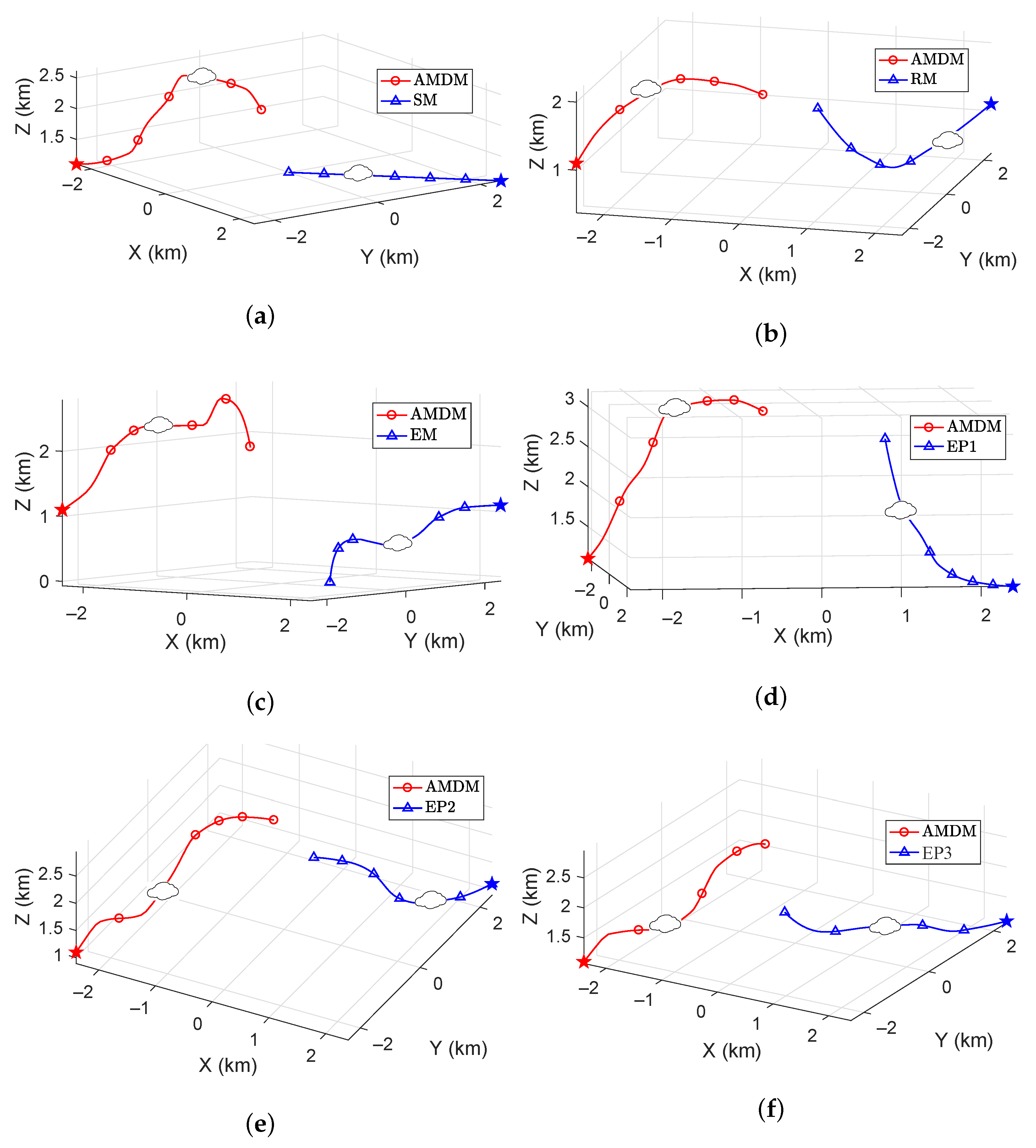
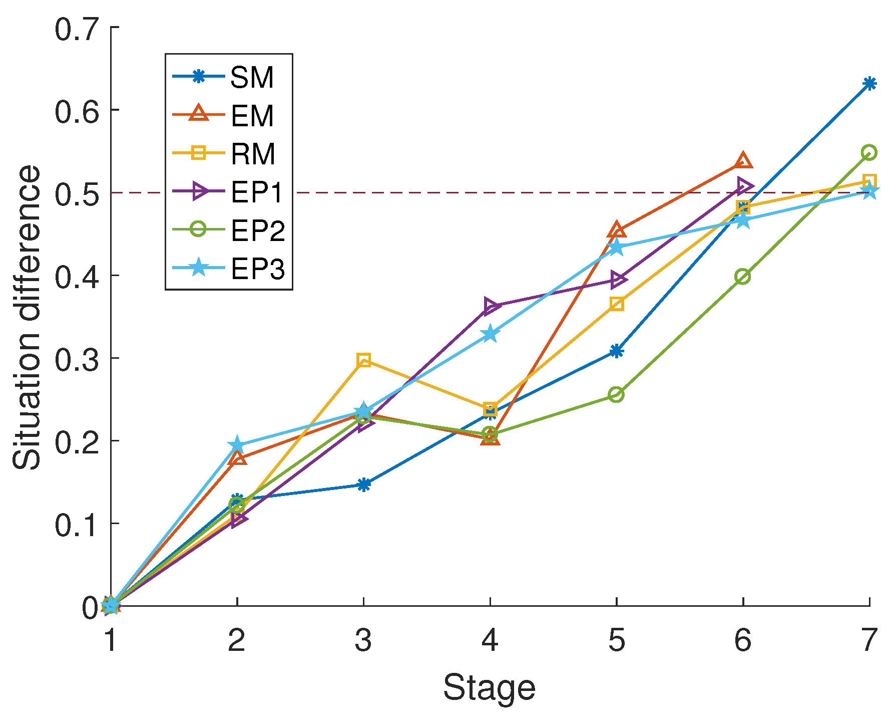
4.2. Some Comparative Experiments of Maneuver Decision-Making Process

In this part, some adversarial experiments of $\mathcal{H}$ and $\mathcal{C}$ are implemented to demonstrate the effectiveness of the proposed algorithm. The initial parameters of $\mathcal{H}$ and $\mathcal{C}$ are first given in

Table 3. Initial parameters of $\mathcal{H}$ and $\mathcal{C}$ of the comparative experiments.

Symbol	Description	$\mathcal{H}$	$\mathcal{C}$
$P_x\left(\mathrm{km}\right)$	X coordinate of position	$2.4$	$-2.4$
$P_y\left(\mathrm{km}\right)$	Y coordinate of position	$2.4$	$-2.4$
$P_z\left(\mathrm{km}\right)$	Z coordinate of position	$1.1$	$1.1$
$V_x(\mathrm{km}·{\mathrm{h}}^{-1})$	X coordinate of speed	$-360$	360
$V_y(\mathrm{km}·{\mathrm{h}}^{-1})$	Y coordinate of speed	$-360$	360
$V_z(\mathrm{km}·{\mathrm{h}}^{-1})$	Z coordinate of speed	0	0
$D_{mi}\left(\mathrm{km}\right)$	Maximum missile launch distance	25	25
$D_{ra}\left(\mathrm{km}\right)$	Maximum radar detection distance	140	140
$V_{mi}\left(\mathrm{Ma}\right)$	Maximum missile speed	4	4
$N_{mi}$	Number of carried missiles	2	2

. These settings ensure that $\mathcal{H}$ and $\mathcal{C}$ have the same situational advantages in the beginning. The simulation step size of these experiments is 4 s.

We assume that $\mathcal{H}$ and $\mathcal{C}$ have the same initial situations and follow the same dynamic model, and that the only difference between them is the algorithm used to maneuver. In these experiments, $\mathcal{C}$ adopts the proposed AMDM algorithm, while $\mathcal{H}$ adopts the existing maneuver strategies or is operated by an experienced person with hand gestures. In order to characterize the partially observable state of $\mathcal{H}$, one state of $\mathcal{H}$ and $\mathcal{C}$ is randomly set to be unobservable, and the data information of these states is artificially deleted. In the unobservable state, our algorithm continues to make maneuver decision-making based on the predicted state of $\mathcal{H}$, while the adversary’s algorithm has no ability to deal with incomplete information. In this case, $\mathcal{H}$ considers that $\mathcal{C}$ took a random maneuver in the previous decision-making stage, so $\mathcal{H}$ makes decisions based on the state of $\mathcal{C}$ after that random maneuver.

The maneuver trajectory of AMDM algorithm compared with other algorithms are shown in Figure 7, where $\mathcal{C}$ adopts the AMDM algorithm, $\mathcal{H}$ respectively adopts the following six maneuver methods: straight maneuver (SM), random maneuver (RM), elemental maneuver (EM) [24], experienced person 1 (EP1), experienced person 2 (EP2), and experienced person 3 (EP3). In each subgraph of Figure 7, the initial positions of $\mathcal{H}$ and $\mathcal{C}$ are marked by the symbol ★, and the unobservable states of $\mathcal{H}$ and $\mathcal{C}$ are covered with clouds. In each experiment, it is considered that $\mathcal{H}$ or $\mathcal{C}$ has reached the ideal attack position, when their situational advantage difference exceeds 0.5.

In the first experiment, $\mathcal{H}$ adopts a fixed straight strategy, and it can be seen form Figure 7a that $\mathcal{C}$ can easily achieve the attack position through the maneuver combination of climbing and diving. In the second experiment, $\mathcal{H}$ takes the random maneuvers. Figure 7b show that the maneuver trajectory of $\mathcal{H}$ when performing random strategy has no regularity, so $\mathcal{C}$ can also loosely complete the attack position. In the third experiment, $\mathcal{H}$ selects an elemental maneuver in the basic maneuver library in each decision-making stage. In Figure 7c, the state information of $\mathcal{C}$ in the third stage is unobservable, which makes $\mathcal{H}$ choose an inappropriate maneuver. As a result, $\mathcal{H}$ gradually loses its situational advantage and finally choses to escape. In the last three experiments, since the experienced person has no ability to predict unobservable states and their decision-making is highly subjective, $\mathcal{H}$ eventually loses priority in angle and height, as shown in Figure 7d, Figure 7e, and Figure 7f, respectively. The situation advantage difference between $\mathcal{C}$ and $\mathcal{H}$ in each stages of these experiments are given in Figure 8, which shows that $\mathcal{C}$ can always outperform $\mathcal{H}$ to reach a favorable attacking position after six to seven decision-making stages. Thus, the effectiveness of the proposed method has been verified.

Furthermore, the back-propagation neural network (BPNN) method is used to predict the unobservable states of $\mathcal{H}$ in the above experiments. In each confrontation experiment, the historical state data of $\mathcal{H}$ is sampled every 1 s, and 8 consecutive data are taken as a sample, where the first 7 are the inputs of the network, and the last one is the target of the network. Then, these samples are randomly divided into a training set, validation set and test set, and their proportions are 70%, 15%, and 15%, respectively. The number of hidden neurons is set to 10, and the Levenberg–Marquardt algorithm is used to train the network. By the above BPNN prediction method, the unobservable state of $\mathcal{H}$ is predicted.

Then, based on the predicted state by BPNN algorithm, the maneuver decision-making game model of this decision-making stage is established, and the corresponding Nash equilibrium strategy is obtained. If the state of $\mathcal{H}$ is unobservable at time $t_i$,

Table 4. Situation advantage change of $\mathcal{C}$ to $\mathcal{H}$ under different state prediction methods.

Algorithm	SM	RM	EM	EP1	EP2	EP3
BPNN	0.1362	0.1459	0.1268	0.0842	0.0971	0.1327
NESP	0.1601	0.1452	0.1312	0.1105	0.1138	0.1492
NESP-BPNN	+0.0239	−0.0007	+0.0026	+0.0263	+0.0167	+0.0165

shows the situation advantage change of $\mathcal{C}$ to $\mathcal{H}$ from $t_{i-1}$ to $t_{i+1}$ under the two state prediction methods. According to Table 4, compared with the BPNN algorithm, the proposed NESP state prediction method can generally enable $\mathcal{C}$ to obtain a higher situation advantage, which shows the effectiveness of the proposed prediction method. This is because the proposed prediction method considers the intentions $\mathcal{H}$, while BPNN only makes predictions based on historical state data.

5. Conclusions

The autonomous maneuver decision-making problem of UCAV under the framework of human-computer gaming has been studied in this paper. The maneuver decision-making process has been decomposed into a sequential decision problem, where each decision-making stage is modeled as a game of $\mathcal{H}$ and $\mathcal{C}$. A continuous maneuver library has been designed, which not only expands the maneuver library to infinity, but also solves the executable problem of mixed strategies. Moreover, the unobservable states in the maneuver decision-making process have been considered, and a state prediction method based on Nash equilibrium has been proposed. Future work will aim to extend the method to the task assignment problem of multiple UCAVs.

References

1. Dalkıran, E.; Önel, T.; Topçu, O.; Demir, K.A. Automated integration of real-time and non-real-time defense systems. Def. Technol. 2021, 17, 657–670. [Google Scholar] [CrossRef]
2. Yang, Z.; Sun, Z.X.; Piao, H.Y.; Huang, J.C.; Zhou, D.Y.; Ren, Z. Online hierarchical recognition method for target tactical intention in beyond-visual-range air combat. Def. Technol. 2022, 18, 1349–1361. [Google Scholar] [CrossRef]
3. Li, S.; Wu, Q.; Chen, M.; Wang, Y. Air Combat Situation Assessment of Multiple UCAVs with Incomplete Information. In CISC 2020: Proceedings of 2020 Chinese Intelligent Systems Conference; Springer: Singapore, 2020; pp. 18–26. [Google Scholar]
4. Guo, J.; Wang, L.; Wang, X. A Group Maintenance Method of Drone Swarm Considering System Mission Reliability. Drones 2022, 6, 269. [Google Scholar] [CrossRef]
5. Shin, H.; Lee, J.; Kim, H.; Shim, D.H. An autonomous aerial combat framework for two-on-two engagements based on basic fighter maneuvers. Aerosp. Sci. Technol. 2018, 72, 305–315. [Google Scholar] [CrossRef]
6. Li, J.; Chen, R.; Peng, T. A Distributed Task Rescheduling Method for UAV Swarms Using Local Task Reordering and Deadlock-Free Task Exchange. Drones 2022, 6, 322. [Google Scholar] [CrossRef]
7. Zhou, X.; Qin, T.; Meng, L. Maneuvering Spacecraft Orbit Determination Using Polynomial Representation. Aerospace 2022, 9, 257. [Google Scholar] [CrossRef]
8. Li, W.; Lyu, Y.; Dai, S.; Chen, H.; Shi, J.; Li, Y. A Multi-Target Consensus-Based Auction Algorithm for Distributed Target Assignment in Cooperative Beyond-Visual-Range Air Combat. Aerospace 2022, 9, 486. [Google Scholar] [CrossRef]
9. Abdar, M.; Pourpanah, F.; Hussain, S.; Rezazadegan, D.; Liu, L.; Ghavamzadeh, M.; Fieguth, P.; Cao, X.; Khosravi, A.; Acharya, U.R.; et al. A review of uncertainty quantification in deep learning: Techniques, applications and challenges. Inf. Fusion 2021, 76, 243–297. [Google Scholar] [CrossRef]
10. Zhang, P.; Wang, C.; Jiang, C.; Han, Z. Deep reinforcement learning assisted federated learning algorithm for data management of IIoT. IEEE Trans. Ind. Inform. 2021, 17, 8475–8484. [Google Scholar] [CrossRef]
11. Du, B.; Mao, R.; Kong, N.; Sun, D. Distributed Data Fusion for On-Scene Signal Sensing With a Multi-UAV System. IEEE Trans. Control Netw. Syst. 2020, 7, 1330–1341. [Google Scholar] [CrossRef]
12. Han, J.; Wu, J.; Zhang, L.; Wang, H.; Zhu, Q.; Zhang, C.; Zhao, H.; Zhang, S. A Classifying-Inversion Method of Offshore Atmospheric Duct Parameters Using AIS Data Based on Artificial Intelligence. Remote Sens. 2022, 14, 3197. [Google Scholar] [CrossRef]
13. Silver, D.; Huang, A.; Maddison, C.J.; Guez, A.; Sifre, L.; Van Den Driessche, G.; Schrittwieser, J.; Antonoglou, I.; Panneershelvam, V.; Lanctot, M.; et al. Mastering the game of Go with deep neural networks and tree search. Nature 2016, 529, 484–489. [Google Scholar] [CrossRef] [PubMed]
14. Brown, N.; Sandholm, T. Superhuman AI for heads-up no-limit poker: Libratus beats top professionals. Science 2018, 359, 418–424. [Google Scholar] [CrossRef] [PubMed] [Green Version]
15. Li, W.; Shi, J.; Wu, Y.; Wang, Y.; Lyu, Y. A Multi-UCAV cooperative occupation method based on weapon engagement zones for beyond-visual-range air combat. Def. Technol. 2022, 18, 1006–1022. [Google Scholar] [CrossRef]
16. Kang, Y.; Pu, Z.; Liu, Z.; Li, G.; Niu, R.; Yi, J. Air-to-Air Combat Tactical Decision Method Based on SIRMs Fuzzy Logic and Improved Genetic Algorithm. In Advances in Guidance, Navigation and Control; Springer: Singapore, 2022; pp. 3699–3709. [Google Scholar]
17. Li, B.; Liang, S.; Chen, D.; Li, X. A Decision-Making Method for Air Combat Maneuver Based on Hybrid Deep Learning Network. Chin. J. Electron. 2022, 31, 107–115. [Google Scholar]
18. Li, S.; Chen, M.; Wang, Y.; Wu, Q. Air combat decision-making of multiple UCAVs based on constraint strategy games. Def. Technol. 2022, 18, 368–383. [Google Scholar] [CrossRef]
19. Zhang, T.; Li, C.; Ma, D.; Wang, X.; Li, C. An optimal task management and control scheme for military operations with dynamic game strategy. Aerosp. Sci. Technol. 2021, 115, 106815. [Google Scholar] [CrossRef]
20. Li, S.; Chen, M.; Wang, Y.; Wu, Q. A fast algorithm to solve large-scale matrix games based on dimensionality reduction and its application in multiple unmanned combat air vehicles attack-defense decision-making. Inf. Sci. 2022, 594, 305–321. [Google Scholar] [CrossRef]
21. Ruan, W.; Duan, H.; Deng, Y. Autonomous Maneuver Decisions via Transfer Learning Pigeon-inspired Optimization for UCAVs in Dogfight Engagements. IEEE/CAA J. Autom. Sin. 2022, 9, 1–19. [Google Scholar] [CrossRef]
22. Hu, J.; Wang, L.; Hu, T.; Guo, C.; Wang, Y. Autonomous Maneuver Decision Making of Dual-UAV Cooperative Air Combat Based on Deep Reinforcement Learning. Electronics 2022, 11, 467. [Google Scholar] [CrossRef]
23. Du, B.; Chen, J.; Sun, D.; Manyam, S.G.; Casbeer, D.W. UAV Trajectory Planning with Probabilistic Geo-Fence via Iterative Chance-Constrained Optimization. IEEE Trans. Intell. Transp. Syst. 2021, 23, 5859–5870. [Google Scholar] [CrossRef]
24. Austin, F.; Carbone, G.; Hinz, H.; Lewis, M.; Falco, M. Game theory for automated maneuvering during air-to-air combat. J. Guid. Control Dyn. 1990, 13, 1143–1149. [Google Scholar] [CrossRef]
25. Yang, Q.; Zhang, J.; Shi, G.; Hu, J.; Wu, Y. Maneuver decision of UAV in short-range air combat based on deep reinforcement learning. IEEE Access 2019, 8, 363–378. [Google Scholar] [CrossRef]
26. Zhang, H.; Huang, C.; Xuan, Y.; Tang, S. Maneuver Decision of Autonomous Air Combat of Unmanned Combat Aerial Vehicle Based on Deep Neural Network. Acta Armamentarii 2020, 41, 1613. [Google Scholar]
27. Li, Y.; Shi, J.; Jiang, W.; Zhang, W.; Lyu, Y. Autonomous maneuver decision-making for a UCAV in short-range aerial combat based on an MS-DDQN algorithm. Def. Technol. 2022, 18, 1697–1714. [Google Scholar] [CrossRef]
28. Hu, D.; Yang, R.; Zhang, Y.; Yue, L.; Yan, M.; Zuo, J.; Zhao, X. Aerial combat maneuvering policy learning based on confrontation demonstrations and dynamic quality replay. Eng. Appl. Artif. Intell. 2022, 111, 104767. [Google Scholar] [CrossRef]
29. Du, B.; Sun, D.; Hwang, I. Distributed State Estimation for Stochastic Linear Hybrid Systems with Finite-Time Fusion. IEEE Trans. Aerosp. Electron. Syst. 2021, 57, 3084–3095. [Google Scholar] [CrossRef]
30. Dong, Y.; Feng, J.; Zhang, H. Cooperative tactical decision methods for multi-aircraft air combat simulation. J. Syst. Simul. 2002, 14, 723–725. [Google Scholar]
31. Jiang, C.; Ding, Q.; Wang, J.; Wang, J. Research on threat assessment and target distribution for multi-aircraft cooperative air combat. Fire Control Command Control 2008, 33, 8–12+21. [Google Scholar]
32. Shen, Z.; Xie, W.; Zhao, X.; Yu, C. Modeling of UAV Battlefield Threats Based on Artificial Potential Field. Comput. Simul. 2014, 31, 60–64. [Google Scholar]
33. Cruz, J.; Simaan, M.A.; Gacic, A.; Liu, Y. Moving horizon Nash strategies for a military air operation. IEEE Trans. Aerosp. Electron. Syst. 2002, 38, 989–999. [Google Scholar] [CrossRef]
34. Maschler, M.; Solan, E.; Zamir, S. Game Theory; Cambridge University Press: Cambridge, UK, 2013. [Google Scholar]
35. Parthasarathy, T.; Raghavan, T.E.S. Some Topics in Two-Person Games; American Elsevier Publishing Company: New York, NY, USA, 1917. [Google Scholar]
36. Huang, C.; Dong, K.; Huang, H.; Tang, S.; Zhang, Z. Autonomous air combat maneuver decision using Bayesian inference and moving horizon optimization. J. Syst. Eng. Electron. 2018, 29, 86–97. [Google Scholar] [CrossRef]
Figure 1. Maneuver decision-making process of H and C .
Drones 07 00157 g001
Figure 2. Air combat situation of H and C .
Drones 07 00157 g002
Figure 3. Overall flow of the maneuver decision-making method of H and C .
Drones 07 00157 g003
Figure 4. All possible maneuvers of H and C .
Drones 07 00157 g004
Figure 5. Prediction of the state of H .
Drones 07 00157 g005
Figure 6. Trajectories of C when performing different maneuvers.
Drones 07 00157 g006
Figure 7. Maneuver trajectories of the AMDM algorithm compared with the other algorithms. (a) Straight maneuver, (b) random maneuver, (c) elemental maneuver, (d) experienced person 1, (e) experienced person 2, (f) experienced person 3.
Drones 07 00157 g007
Figure 8. The difference between the situation advantages of C and H .
Drones 07 00157 g008