A Hybrid Improved Symbiotic Organisms Search and Sine–Cosine Particle Swarm Optimization Method for Drone 3D Path Planning

Abstract

Given the accelerated advancement of drones in an array of application domains, the imperative of effective path planning has emerged as a quintessential research focus. Particularly in intricate three-dimensional (3D) environments, formulating the optimal flight path for drones poses a substantial challenge. Nonetheless, prevalent path-planning algorithms exhibit issues encompassing diminished accuracy and inadequate stability. To solve this problem, a hybrid improved symbiotic organisms search (ISOS) and sine–cosine particle swarm optimization (SCPSO) method for drone 3D path planning named HISOS-SCPSO is proposed. In the proposed method, chaotic logistic mapping is first used to improve the diversity of the initial population. Then, the difference strategy, the novel attenuation functions, and the population regeneration strategy are introduced to improve the performance of the algorithm. Finally, in order to ensure that the planned path is available for drone flight, a novel cost function is designed, and a cubic B-spline curve is employed to effectively refine and smoothen the flight path. To assess performance, the simulation is carried out in the mountainous and urban areas. An extensive body of research attests to the exceptional performance of our proposed HISOS-SCPSO.

1. Introduction

Catastrophic incidents like flash floods and earthquakes frequently result in substantial damage and casualties within the impacted regions. During such occurrences, the need for prompt disaster relief operations becomes paramount, as any delay could amplify the toll on human lives and property. In the face of such an emergency, how to quickly and efficiently carry out emergency rescue [1] has ascended to a paramount concern. However, owing to the disrupted traffic flow and deteriorated road conditions after a disaster, it is difficult for rescue teams to promptly access disaster regions. In recent times, the swift advancement of drone technology has significantly contributed to various domains, including the military [2], agriculture [3], meteorology [4], and transportation [5]. Simultaneously, it has also presented novel avenues for addressing disaster relief challenges [6]. Drones exhibit attributes of flexibility, speed, and efficiency, enabling them to swiftly traverse over afflicted regions, conduct assessments of the extent of damage [7], and furnish precise data to inform rescue-related decisions. Furthermore, they facilitate the expeditious delivery of relief provisions to disaster areas [8], effectively addressing the immediate necessities of those affected. Therefore, drone-based disaster rescue aligns with the exigency of emergency response and can greatly reduce the losses caused by disasters [9]. As a key part of drone disaster relief, path planning is crucial at this moment [10,11]. The drone’s path planning entails formulating a flight path that incurs minimal costs while adhering to a spectrum of constraints. Numerous factors exert influence on drone path planning [12], including terrain, obstacle considerations, and body performance limitations (such as the maximum turning angle). Therefore, within the context of disaster rescue operations, the central research focus pertains to devising an optimal path for the drone, ensuring its secure navigation to the designated mission point.

Currently, a multitude of methodologies have emerged to solve the path-planning problem [13,14], which are mainly classified into five categories.

Table 1. The summary of path-planning algorithms.

Algorithm Category	Representative Approach
Mathematical Model-Based Method	Dynamic programming (DP) [15], mixed-integer linear programming (MILP) [16], etc.
Sampling-Based Search Method	Probabilistic roadmap (PRM) [17], rapidly-exploring random tree (RRT) [18], etc.
Node-Based Search Method	Dijkstra algorithm [19], A-star (A*) [20], harmony search (HS) [21], etc.
Artificial Potential Field Method	Artificial potential field (APF) [22], improved artificial potential field (IAPF) [23], etc.
Evolutionary Method	Symbiotic organisms search (SOS) [24], particle swarm optimization (PSO) [25], differential evolution (DE) [26], etc.

shows the summary of path-planning algorithms. The mathematical model-based method [15,16] abstracts the path-planning problem into a mathematical expression and uses the mathematical solution method to find the optimal path through the objective function and constraints. The sampling-based search method [17,18] gradually explores and optimizes the path to obtain the optimal path by generating sampling points in continuous space, fully considering environmental constraints, and using tree-like structures or optimization techniques. The node-based search method [19,20,21] abstracts the problem into graphs, networks, or state spaces, leveraging graph theory to plan the optimal path; sometimes, combined with the heuristic evaluation function, the path length and the estimated target distance are comprehensively considered for path search. The artificial potential field method [22,23] is a path-planning approach grounded in the concept of potential energy. It achieves obstacle avoidance and target reaching by defining attractive and repulsive potential energies. The evolutionary algorithm [24,25,26] is a method of simulating natural biological clusters and evolution. It continuously optimizes the solution through fitness evaluation and evolution to achieve the optimal path.

Due to the inherent nondeterministic polynomial (NP) completeness of path-planning problems, population-based heuristic algorithms have been extensively employed to tackle such issues. Currently, researchers have employed various heuristic algorithms to address path-planning problems and have achieved remarkable advancements. In [27], the iterative process of the global optimal solution of PSO was combined with the annealing simulation (SA) algorithm to reduce the particle oscillation phenomenon in the iterative process. In [28], the adaptive transformation acceleration coefficients and mutation strategies were introduced into PSO to realize the path planning of drone formation. In [29], a hybrid algorithm termed HSGWO-MSOS combining simplified grey wolf optimizer and modified SOS was designed to achieve the optimal path planning of drones in field environments. In [30], a modified SOS based on the simplex method (SMSOS) was proposed to address the challenge of finding the shortest path for unmanned combat aircraft vehicles in a random battlefield environment. In [31], an adaptive selection mutation constrained DE considering flight distance and risk was developed, which was suitable for the path planning of drones in disaster scenarios. In [32], a fuzzy adaptive DE for drone path planning was created that aims to minimize energy consumption and threat factors. In [33], a path-planning method based on an improved genetic algorithm (IGA) was devised. The strategy of multi-domain inversion to increase the number of offspring was employed in IGA to overcome the defects of premature and slow convergence speed of the original genetic algorithm. In [34], four adaptive adjustment factors were introduced into the ant colony algorithm, and an improved adaptive ant colony algorithm (IAACO) with high real-time stability was proposed.

Nevertheless, despite the widespread application of population-based heuristic algorithms, these algorithms still suffer from drawbacks such as diminished accuracy and inadequate stability. Although various variants of heuristic algorithms have been designed in existing research and have shown promising progress in the field of path planning, there are still some shortcomings that need to be addressed: First, striking a balance between the global exploration and local exploitation capabilities of heuristic algorithms poses a challenge, and these two capabilities are crucial factors in evaluating the effectiveness of heuristic algorithms [35]. Second, although the fusion variant can obtain better optimization ability, it overlooks the significant rise in computational time, severely compromising the real-time performance of the algorithm. Third, the majority of existing research has been conducted in custom simple 2D scenarios without considering complex real-world 3D environments, which makes it difficult to apply the research to the path planning of drones in real 3D scenes.

In this paper, a novel method called HISOS-SCPSO is presented for 3D path planning of drones in disaster relief scenarios. First, the B-spline curve is described and employed to represent the flight path of the drone. Second, two common disaster rescue scenarios are constructed, including mountainous terrain and urban settings. Third, a cost function considering the drone’s flight distance, flight altitude, flight environment, turning cost, and its own performance characteristics is constructed. Finally, the proposed HISOS-SCPSO is employed to address the issue of drone 3D path planning. The algorithm first employs a chaotic logistics mapping to optimize the quality of the initial solution. Subsequently, the mutualism phase of SOS is improved and merged with SCPSO. It preserves the SOS’s strong local exploitation capability while enhancing its global exploration capability. Moreover, the difference strategy is introduced to replace the individual cognitive part in SCPSO to improve the convergence ability and improve the accuracy of the algorithm. To balance the algorithm’s global and local optimization abilities, new attenuation functions are proposed. Additionally, a strategy of population regeneration is designed to ensure algorithm stability.

The main contributions of this paper include (1) the development of a novel model for drone path planning in disaster rescue scenarios. The representation method for the flight path is defined, along with the characterization of mountainous terrain and urban environments. A cost function considering various costs and drone performance is established. (2) A new path-planning method, HISOS-SCPSO, is proposed. The method integrates two improved algorithms, incorporating multiple optimization strategies to enhance its optimization capabilities while ensuring computational efficiency. (3) The proposed HISOS-SCPSO is applied to 3D real terrain simulation, successfully achieving drone path planning within intricate and authentic 3D environments.

In the following sections, first, the modeling approach for drone path planning will be designed in Section 2. Second, a comprehensive exploration of the population initialization method based on chaotic logistics mapping is introduced in Section 3, as well as the fundamental principles of PSO, SOS, and HISOS-SCPSO. Third, a series of comparative experiments are conducted in Section 4. Finally, the conclusion is given in Section 5.

2. Drone Path Planning Modeling

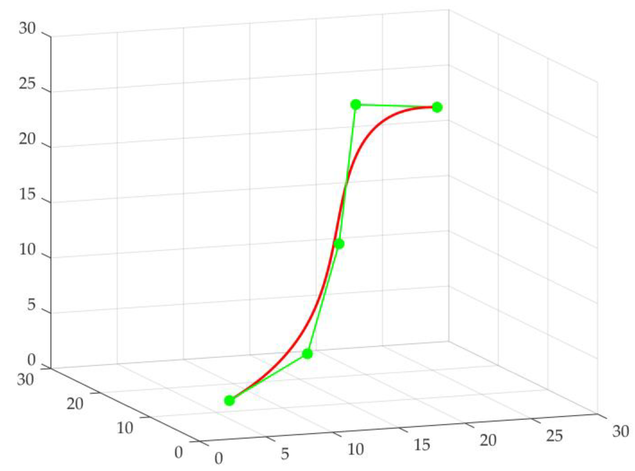
2.1. Path Representation Method

Generally, the optimization results of evolutionary algorithms consist of a series of path points. Directly connecting these path points with straight lines will not be suitable for drone flight. B-spline curves, evolved from Bezier curves, are a common curve representation method [36]. They define the curve shape through control points, node vectors, and basis functions and have the characteristics of smoothness, flexibility, and local control. Defined with just a few parameters, B-spline curves are well-suited for smoothing the results of evolutionary algorithm optimization into feasible flight paths [37]. Therefore, in order to obtain a smooth and flyable path, B-spline curves are introduced for drone path planning in this paper.

Suppose that the drone flies from the starting point P₀ = (X₀, Y₀, Z₀) to the target point P_n = (X_n, Y_n, Z_n), where P_{1, n-1} = [(X₁, Y₁, Z₁), (X₂, Y₂, Z₂), …, (X_n−1, Y_n−1, Z_n−1)] means the control point of the output of the evolutionary algorithm. Then, the coordinates of the B-spline curve generated by n + 1 control points are B_{0, s} = [(x₀, y₀, z₀), (x₁, y₁, z₁), …, (x_s, y_s, z_s)], that is, the drone path point, and the calculation can be formulated as shown in Equation (1).

$$\left\{\begin{array}{l}{x}_j={\displaystyle \sum _{i=0}^n{X}_i\cdot B_{i,k}\left(t_j\right)}\\ y_j={\displaystyle \sum _{i=0}^n{Y}_i\cdot B_{i,k}\left(t_j\right)}\\ z_j={\displaystyle \sum _{i=0}^n{Z}_i\cdot B_{i,k}\left(t_j\right)}\end{array}\right. j=0,1,2,\dots ,s$$

(1)

where (x_j, y_j, z_j) represents the coordinates of the jth path point, and (X_i, Y_i, Z_i) is the coordinates of the control points; k signifies the degree of the B-spline curve, reflecting its smoothness. A higher k value generates a smoother B-spline curve. The symbol t is a discrete sequence with a constant step length ranging from 0 to n + k + 1, and t_j represents the jth discrete value in this sequence. The symbol B_i,k denotes the ith k-degree B-spline basis function, defined recursively by Cox–deBoor, as depicted in Equations (2) and (3).

$$B_{i,1}\left(t_j\right)=\left\{\begin{array}{l}1, u_i\le t_j<u_{i+1}\\ 0, otherwise\end{array}\right.$$

(2)

$$B_{i,k}\left(t_j\right)=\frac{t_j-u_i}{u_{i+k-1}-u_i}{B}_{i,k-1}\left(t_j\right)+\frac{u_{i+k}-t_j}{u_{i+k}-u_{i+1}}{B}_{i+1,k-1}\left(t_j\right)$$

(3)

where (u₀, u₁, u₂, …, u_n+k) represents the knot vector formed by a non-decreasing sequence. Uniform non-periodic knot vectors are the most commonly used, and their calculation is depicted in Equation (4).

$$u_i=\left\{\begin{array}{ll}0,& i\le k\\ i-k,& k<i\le s-1\\ s-k,& s\le i\end{array}\right.$$

(4)

In this paper, the degree of the B-spline curve is set to k = 3. Figure 1 is the result of smoothing the five control points through the B-spline curve, and the generated curve is a flyable path.

2.2. The Modeling Methods of Flight Environment

Due to the frequent occurrence of disaster events in mountainous and urban regions, drone flights are often influenced by topographical features such as mountains and architectural structures. Without accurate models of these mountains and buildings, the survivability of drones could be significantly compromised. Therefore, modeling these two types of environments is of utmost importance.

2.2.1. The Mountain Environment

The 3D simulation of mountain terrain consists of the original terrain and mountain obstacles, and the model of the original terrain is constructed by Equation (5) [38].

$$z_1(x,y)=sin(y+a)+b sin(x)+c cos(y)+d cos(e\sqrt{x^2+y^2})+f sin(f\sqrt{x^2+y^2})$$

(5)

where (x, y) denotes the coordinates of a point on the horizontal plane, and z₁(x, y) represents the corresponding terrain height. The parameters a, b, c, d, e, and f are terrain coefficients. These parameters influence the degree of terrain undulation, and different combinations can simulate various terrain features. In this paper, the terrain parameters are set to a = 3 π, b = 5, c = 2, d = 4, e = 3, and f = 1.

The mathematical model for mountain obstacles is presented by Equation (6).

$$z_2(x,y)={\displaystyle \sum _{i_m=1}^{N_m}{h}_m\left(i_m\right)\cdot exp\left[-{\left(\frac{x-x_0\left(i_m\right)}{x_{sl}\left(i_m\right)}\right)}^2-{\left(\frac{y-y_0\left(i_m\right)}{y_{sl}\left(i_m\right)}\right)}^2\right]}$$

(6)

where z₂(x, y) represents the height of point (x, y) corresponding to the mountain obstacles, N_m is the total number of mountain obstacles, and h_m(i_m) denotes the height of the i_mth mountain obstacle. The symbol (x₀(i_m), y₀(i_m)) is the central coordinate of the i_mth mountain obstacle on the horizontal plane, and x_sl(i_m) and y_sl(i_m) are the slope parameters along the x and y axes for the i_mth mountain obstacle. By adjusting h_m(i_m), x_sl(i_m), and y_sl(i_m), various profiles of mountain obstacles can be constructed.

Finally, the original terrain and mountain obstacles are merged to form a 3D simulated mountain terrain according to Equation (7).

$$z_m(x,y)=max\left[z_1(x,y),k_m{z}_2(x,y)\right]$$

(7)

where z_m(x, y) represents the height of the 3D simulated mountain terrain corresponding to point (x, y). The symbol max means the maximum value function, and k_m is the terrain adjustment coefficient, which is set to k_m = 10 in this study.

2.2.2. The Urban Environment

The three-dimensional simulated urban terrain primarily consists of high-rise buildings. We approximate the obstacles in the 3D urban simulation as various prisms. Assuming that the urban environment ground is completely horizontal, the elevation model for the entire city can be represented using Equation (8).

$$z_u(x,y)=\left\{\begin{array}{ll}{h}_u\left(i_u\right),& if\left(x,y\right)\in O_u\left(i_u\right)\\ 0,& otherwise\end{array}\right.$$

(8)

where z_u(x, y) represents the height of the 3D simulated urban terrain corresponding to the point (x, y), and h_u(i_u) is the height of the i_uth urban obstacle. The symbol O_u(i_u) denotes the base of the i_uth urban obstacle, formed by connecting the vertices of the i_uth urban obstacle’s base [(x_u,1(i_u), y_u,1(i_u)), (x_u,2(i_u), y_u,2(i_u)), …, (x_{u, Niu}(i_u), y_{u, Niu}(i_u))] sequentially; Niu is the number of vertices of the base of the i_uth urban obstacle.

2.3. The Cost Function of Optimization Method

The cost function is a mathematical model in path planning, which is utilized to balance various factors and quantify the quality of paths. In this paper, the design of the cost function takes into account several factors, including flight distance, flight altitude, and the cost of path smoothness, as well as constraints related to collision avoidance, minimum and maximum flight altitudes, maximum horizontal turn angles, and maximum climb slopes.

2.3.1. Flight Distance Cost

Due to the urgency of disaster relief operations, it is crucial for drones to reach the disaster area as quickly as possible. In such scenarios, the planned path should be as short as possible. The drone’s path is composed of multiple path points, and the cost of flight distance can be represented as shown in Equation (9).

$$C_{distance}={\displaystyle \sum _{j=0}^{s-1}\sqrt{{\left(x_{j+1}-x_j\right)}^2+{\left(y_{j+1}-y_j\right)}^2+{\left(z_{j+1}-z_j\right)}^2}}$$

(9)

where C_distance represents the cost of flight distance, and (x_j, y_j, z_j) denotes the coordinates of the jth path point.

2.3.2. Flight Altitude Cost

In disaster relief scenarios, energy consumption is a crucial factor that must be taken into account. Besides the necessity of minimizing the flight distance, minimizing altitude variations during drone flight also contributes to reducing energy consumption. The cost of drone flight altitude is represented by Equation (10).

$$C_{height}={\displaystyle \sum _{j=0}^{s-1}\left|z_{j+1}-z_j\right|}$$

(10)

where C_height represents the cost of flight altitude, and z_j is the altitude of the jth path point.

2.3.3. Path Smoothness Cost

The smoother the path of the drone during flight, which means reducing the total turning angles of the drone, the more advantageous it is for reducing energy consumption. The cost of path smoothness is represented by the sum of angles between flight segments, as shown in Equation (11).

$$C_{smooth}={\displaystyle \sum _{j=0}^{s-2}arccos\frac{{\phi }_{j+1}{\phi }_j}{\left|{\phi }_{j+1}\right|\cdot \left|{\phi }_j\right|}}$$

(11)

where C_smooth represents the cost of path smoothness, and φ_j denotes the vector of the flight segment (x_j+1 − x_j, y_j+1 − y_j, z_j+1 − z_j).

2.3.4. Collision Avoidance Constraint

During the drone flight, the foremost consideration is to ensure that it does not collide with the terrain or obstacles. The constraints for collision avoidance are represented by Equations (12) and (13).

$$C_{collision}={\displaystyle \sum _{j=1}^{s-1}{Q}_{col,j}}$$

(12)

$$Q_{col,j}=\left\{\begin{array}{ll}{k}_{col},& if \left(x_j,y_j,z_j\right) is in obstacles\\ 0,& otherwise\end{array}\right.$$

(13)

where C_collision represents the cost of path collision, Q_col,j is the violation of collision constraints for the jth path point (x_j, y_j, z_j), and k_col is the coefficient for collision constraint violation, which is set to k_col = 20 in this paper.

2.3.5. Minimum Flight Altitude Constraint

During drone flight, it is essential to maintain a safe distance above the ground to avoid collisions with pedestrians, vehicles, trees, and other obstacles. The constraints for minimum flight altitude are represented by Equations (14) and (15).

$$C_{\mathit{min}f}={\displaystyle \sum _{j=1}^{s-1}{Q}_{\mathit{min}f,j}}$$

(14)

$$Q_{\mathit{min}f,j}=\left\{\begin{array}{ll}{k}_{\mathit{min}f},& if z_j-z_m\left(x_j,y_j\right)<z_{\mathit{min}} or z_j-z_u\left(x_j,y_j\right)<z_{\mathit{min}}\\ 0,& otherwise\end{array}\right.$$

(15)

where C_minf represents the cost of minimum flight altitude, Q_minf,j is the violation of minimum flight altitude constraints for the jth path point (x_j, y_j, z_j), and k_minf is the coefficient of minimum flight altitude constraint violation, which is set to k_minf = 20 in this paper. The symbols z_m(x_j, y_j) and z_u(x_j, y_j) represent the elevation of mountainous terrain and urban terrain at the coordinates (x_j, y_j), respectively. The symbol z_min denotes the minimum safe flight distance, which is set to z_min = 10 in this paper.

2.3.6. Maximum Flight Altitude Constraint

During drone flight, ensuring safety and compliance with airspace regulations, including air traffic control in the planning area, requires the drone to maintain its altitude below a certain threshold. The constraints for maximum flight altitude are represented by Equations (16) and (17).

$$C_{\mathit{max}f}={\displaystyle \sum _{j=1}^{s-1}{Q}_{\mathit{max}f,j}}$$

(16)

$$Q_{\mathit{max}f,j}=\left\{\begin{array}{ll}{k}_{\mathit{max}f},& if z_j>z_{\mathit{max}} \\ 0,& otherwise\end{array}\right.$$

(17)

where C_maxf represents the cost of maximum flight altitude, Q_maxf,j is the violation of maximum flight altitude constraints for the jth path point (x_j, y_j, z_j), and k_maxf is the coefficient for violation of maximum flight altitude constraints, which is set to k_maxf = 20 in this paper. The symbol z_max denotes the maximum flight altitude, which is set to z_max = 800 in this paper.

2.3.7. Maximum Horizontal Turn Angles Constraint

Constrained by its inherent maneuvering capabilities, a drone can only perform turns within a certain angle range in the horizontal direction. The constraints for the maximum horizontal turning angle are represented by Equations (18) and (19).

$$C_{hor}={\displaystyle \sum _{j=1}^{s-1}{Q}_{hor,j}}$$

(18)

$$Q_{hor,j}=\left\{\begin{array}{ll}{k}_{hor},& otherwise \\ 0,& if 0\le {\alpha }_j\le {\alpha }_{\mathit{max}}\end{array}\right.$$

(19)

where C_hor represents the cost of maximum horizontal turning angle, Q_hor,j denotes the violation of the maximum horizontal turning angle constraint for the jth horizontal turning angle, and k_hor is the coefficient for violation of the maximum horizontal turning angle constraint, which is set to k_hor = 20 in this study. The symbol α_j indicates the jth horizontal turning angle, and its calculation is determined by Equation (20); α_max is the maximum allowable horizontal turning angle and is set to α_max = 45° in this paper.

$${\alpha }_j=arccos\frac{\left(x_j-x_{j-1}\right)\cdot \left(x_{j+1}-x_j\right)+\left(y_j-y_{j-1}\right)\cdot \left(y_{j+1}-y_j\right)}{\sqrt{{\left(x_j-x_{j-1}\right)}^2+{\left(y_j-y_{j-1}\right)}^2}\cdot \sqrt{{\left(x_{j+1}-x_j\right)}^2+{\left(y_{j+1}-y_j\right)}^2}}$$

(20)

2.3.8. Maximum Climbing Slopes Constraint

Similarly, analogous to the constraint on the maximum horizontal turning angle, the drone is limited to a certain angle range for climbing in the vertical direction. The maximum climbing slopes constraint is expressed as shown in Equations (21) and (22).

$$C_{ver}={\displaystyle \sum _{j=1}^s{Q}_{ver,j}}$$

(21)

$$Q_{ver,j}=\left\{\begin{array}{ll}{k}_{ver},& otherwise \\ 0,& if 0\le {\beta }_j\le {\beta }_{\mathit{max}}\end{array}\right.$$

(22)

where C_ver represents the cost of the maximum climbing slope, Q_ver,j denotes the violation of the maximum climbing slope constraint for the jth climbing slope, and k_ver is the violation coefficient for the maximum climbing slope constraint, which is set to k_ver = 20 in this study. The symbol β_j means the jth climbing slope, calculated as shown in Equation (23); β_max indicates the maximum climbing slope, which is set to β_max = 45° in this study.

$${\beta }_j=arctan\frac{\left|z_j-z_{j-1}\right|}{\sqrt{{\left(x_j-x_{j-1}\right)}^2+{\left(y_j-y_{j-1}\right)}^2}}$$

(23)

Finally, the cost function is defined as shown in Equations (24) and (25).

$$C_{all}=k_1\cdot C_{distance}+k_2\cdot C_{height}+k_3\cdot C_{smooth}+C_{constraint}$$

(24)

$$C_{constraint}=C_{collision}+C_{minf}+C_{maxf}+C_{hor}+C_{ver}$$

(25)

where C_all represents the total cost of the path planning, C_constraint is the constraint cost, k₁ is the weight for flight distance cost, k₂ denotes the weight for flight height cost, and k₃ indicates the weight for path smoothness cost. In this study, the values are set to k₁ = 1/20, k₂ = 1/15, and k₃ = 1.

3. Optimization Method

3.1. The Basic PSO

The PSO is a heuristic optimization algorithm inspired by natural phenomena like bird flocking. In PSO, candidate solutions are represented as particles, each having a position, velocity, and fitness value, representing a solution, search direction, and value of the solution, respectively. These particles move through the solution space, leveraging individual and collective experiences to find the optimal solution. The basic computation of particle velocity and position in PSO is illustrated by Equations (26) and (27).

$$v_{ip,tp+1}=w_p\cdot v_{ip,tp}+c_{1p}\cdot r_{1p}\cdot \left(P_{bestp,ip}-x_{ip,tp}\right)+c_{2p}\cdot r_{2p}\cdot \left(G_{bestp}-x_{ip,tp}\right)$$

(26)

$$x_{ip,tp+1}=x_{ip,tp}+v_{ip,tp+1}$$

(27)

where v_ip,tp and x_ip,tp denote the velocity and position of the ipth particle in the tpth generation, respectively; w_p, c_1p, and c_2p represent the inertia weight coefficient, individual acceleration coefficient, and group acceleration coefficient, respectively; and r_1p and r_2p are random values within the range [0, 1]. The symbol P_bestp,ip signifies the best position of the ipth particle; G_bestp is the global best position of the particles.

Each particle adjusts its own position and velocity based on its own historical best performance and the overall best performance of the entire group, gradually approaching the optimal solution. Through continuous iterations, PSO can search for better solutions to complex problems.

3.2. The Basic SOS Algorithm

SOS is a heuristic optimization algorithm that seeks the optimal solution to a problem by simulating the symbiotic relationships among organisms in the natural world. In SOS, each solution is treated as an individual organism, and the quality of the solution reflects the fitness of that organism. In each iteration of the algorithm, every organism attempts to change its state (i.e., the value of the solution) in order to improve its fitness through simulated interactions resembling symbiotic relationships. SOS consists of three stages: mutualism, commensalism, and parasitism.

In the mutualism stage, each individual S_p in the population randomly selects another individual S_q and engages in mutual interaction to generate two new individuals, following Equations (28)–(30).

$$S_{pnew}=S_p+r_{1s}\cdot \left(S_{best}-MV\cdot B{F}_1\right)$$

(28)

$$S_{qnew}=S_q+r_{2s}\cdot \left(S_{best}-MV\cdot B{F}_2\right)$$

(29)

$$MF=\frac{S_p+S_q}{2}$$

(30)

where S_pnew and S_qnew denote the generated new individuals; r_1s and r_2s are random values in the range [0, 1]. The symbol S_best indicates the current best individual. The symbol MV represents the mutualism vector; BF₁ and BF₂ mean benefit factors randomly chosen as 1 or 2. Individual updates are only performed when the generated new individuals are superior to the original individuals.

In the commensalism phase, individual S_p within the population endeavors to attain a new state by leveraging the influence of another individual S_q, aiming to enhance its own fitness while not affecting individual S_q. The update of individual S_p occurs only when the fitness of the new state surpasses that of the original state. This stage can be described by Equation (31).

$$S_{pnew}=S_p+r_{3s}\cdot \left(S_{best}-S_q\right)$$

(31)

where r_3s is a random value within the range [−1, 1].

In the parasitism phase, a random individual S_p is selected, and then a random modification is applied to a chosen dimension. The newly generated individual is compared in terms of fitness with another individual S_q in the population. If the newly generated individual exhibits better fitness, the host individual S_q will be replaced by the new individual.

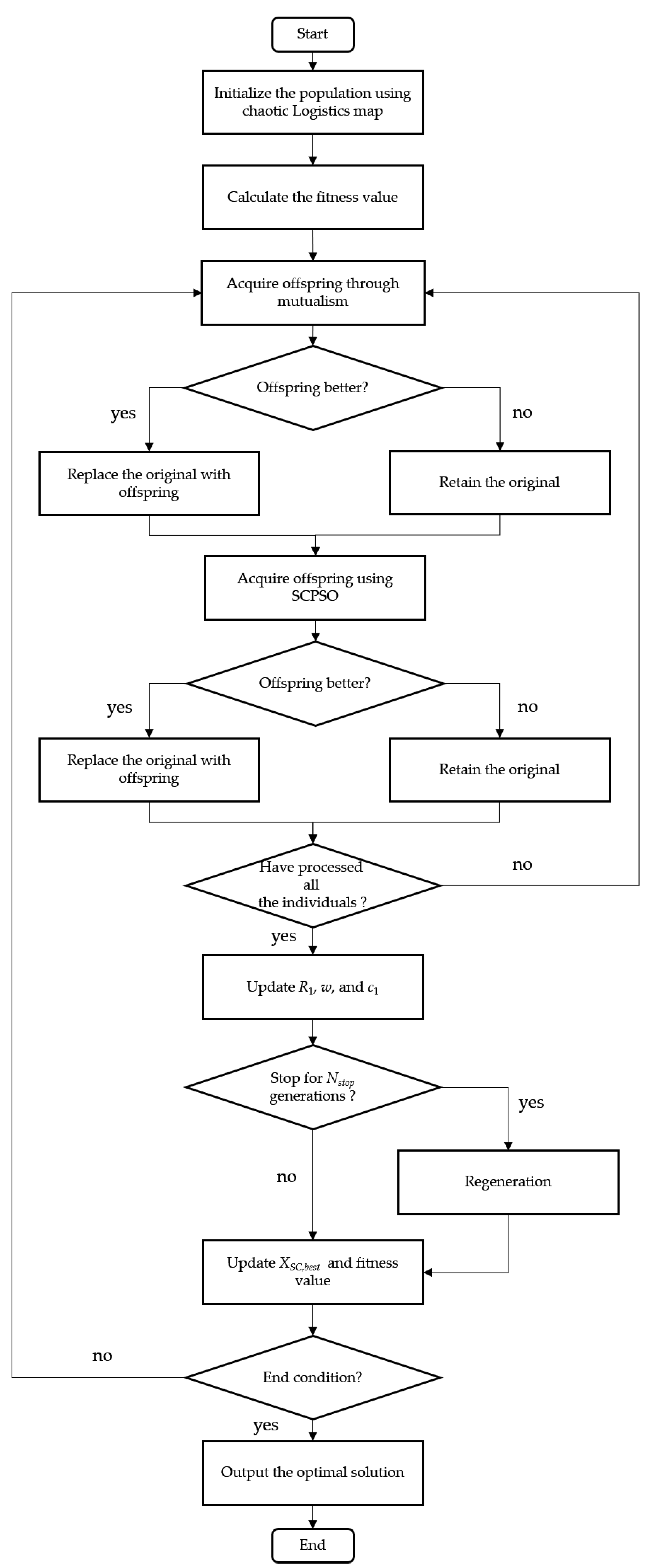
3.3. The Proposed HISOS-SCPSO Method

In PSO, particles adjust their velocities and positions based on their individual best solutions and the global best solution. This guidance from collective information allows PSO to efficiently explore a large search space, which is helpful in finding the global optimal solution. As a result, the PSO has a strong ability in global exploration. However, due to limited information exchange among particles, adjustments based on individual best solutions might lead particles to prematurely converge to local optima. Therefore, PSO exhibits limitations in local exploitation capabilities. On the other hand, SOS leverages interactions among individuals to excel in local exploitation, which helps avoid some of the issues faced by PSO. Our previous research has demonstrated that SCPSO outperforms PSO in optimization missions [39]. Consequently, in order to better solve the 3D path-planning problem of drones, SOS is improved and combined with SCPSO, and various optimization strategies are introduced to propose a new algorithm, HISOS-SCPSO, in this paper.

The optimization results of evolutionary algorithms are influenced by the initial distribution of the population. A more evenly distributed population in the solution space increases the chances of finding the optimal solution, reduces the probability of getting stuck in local optima, and accelerates convergence. The chaotic logistic map is a mathematical mapping function based on chaos theory, characterized by high randomness and disorder. Its calculation method is shown in Equation (32) [40]. Compared to random initialization, using the logistic map to initialize the population can provide better diversity and randomness in the initial stages of the evolutionary algorithm. To enhance the diversity of the initial population, the logistic map is employed for population initialization in this paper.

$$x_{n+1}^{\prime }=\mu \cdot x_n^{\prime }\cdot \left(1-x_n^{\prime }\right)$$

(32)

where μ is the control parameter, typically chosen within the range of [3.57, 4], which corresponds to the chaotic state of the system, and $x_n^{\prime }$ represents the nth chaotic variable. In this paper, μ is set to 4, and $x_0^{\prime }$ is initialized within the range (0, 1), leading the system to uniformly generate chaotic signals.

Since the mutualism phase of SOS demonstrates robust optimization capabilities, it is retained in HISOS-SCPSO. In this step, individual X_SC,p interacts with another randomly chosen individual X_SC,q, generating a mutualism vector MV_SC that influences X_SC,p to generate a new offspring. This procedure can be described using Equations (33) and (34).

$$X_{SC,pq\_new}=X_{SC,p}+r_{SC}\cdot \left(X_{SC,best}-M{V}_{SC}\cdot B{F}_{SC}\right)$$

(33)

$$M{V}_{SC}=\frac{X_{SC,p}+X_{SC,q}}{2}$$

(34)

where X_{SC,pq_new} represents the newly generated individual; r_SC is a random value within the range [0, 1]. The symbol X_SC,best is the current best individual; MV_SC denotes the mutualism vector; BF_SC is the benefit factor randomly chosen as 1 or 2. The newly generated individual is only adopted to replace the X_SC,p if it exhibits better fitness. Compared to SOS, HISOS-SCPSO generates only one new individual in this phase, resulting in a significant reduction in computational effort.

The second part of HISOS-SCPSO involves the optimization of PSO. Sine and cosine factors are introduced to enhance the algorithm’s optimization capability. Additionally, to improve the convergence ability of the algorithm, we modify the cognitive part of SCPSO from the difference between the individual best and the current individual to the difference between two distinct individuals. The SCPSO augmented with difference strategy is presented in Equations (35)–(38). To balance the algorithm’s global exploration and local exploitation abilities, novel attenuation functions are proposed for the inertia coefficient and individual acceleration coefficients, as shown in Equations (39)–(41).

$$V_{SC,pnew}=w\cdot V_{SC,p}+c_1\cdot r_1\cdot \left(X_{SC,q}-X_{SC,p}\right)+k_{SC}$$

(35)

$$k_{sc}=\left\{\begin{array}{l}{R}_1\cdot sin\left(R_2\right)\cdot \left(R_3\cdot X_{SC,best}-X_{SC,p}\right), R_4<0.5\\ R_1\cdot cos\left(R_2\right)\cdot \left(R_3\cdot X_{SC,best}-X_{SC,p}\right), R_4\ge 0.5\end{array}\right.$$

(36)

$$R_1=1-\frac{t}{T}$$

(37)

$$X_{SC,pnew}=X_{SC,p}+k_v\cdot V_{SC,pnew}$$

(38)

$$\lambda =exp\left(1-\frac{T}{1+T-t}\right)$$

(39)

$$w=\left[\frac{w_{\mathit{max}}}{2}-(\frac{w_{\mathit{max}}}{2}-w_{\mathit{min}})\cdot \frac{t}{T}\right]\cdot 2^{\lambda }$$

(40)

$$c_1=c_{1\mathit{max}}-(c_{1\mathit{max}}-c_{1\mathit{min}})\cdot \frac{t}{T}$$

(41)

where V_SC,p and X_SC,p represent the velocity and position of the pth particle, and V_SC,pnew and X_SC,pnew are their respective offspring. The symbol w is the inertia weight coefficient; c₁ is the individual acceleration coefficient; r₁ is a random number in the range [0, 1]; k_SC demotes the sine and cosine component; and R₁ signifies the amplitude control parameter, which is adaptively adjusted through Equation (37). The parameters R₂, R₃, and R₄ are uniformly distributed random numbers, with R₂∈(0, π/2), R₃∈(0, 2), and R₄∈(0, 1) in this study; t represents the current iteration; and T is the maximum number of iterations. The symbol k_v means the velocity factor and is set to k_v = 0.75; λ denotes the inertia attenuation factor; and w_max and w_min are the maximum and minimum values of the inertia weight, which are set to w_max = 0.9 and w_min = 0.15. The symbols c_1max and c_1min represent the maximum and minimum values of the individual acceleration coefficient, which are set as c_1max = 2.5 and c_1min = 0.5. The fitness of the parent X_SC,p and the offspring X_SC,pnew are compared, and only if the offspring’s fitness is better than the parent’s will the offspring replace the parent; otherwise, the parent is retained for the next generation.

The final strategy employed by HISOS-SCPSO is population regeneration. When evolution stagnates for a certain number of generations N_stag, all individuals in the population are arranged based on their fitness, and the N_worst individuals with the lowest fitness are removed. Simultaneously, an equal number of new individuals are randomly generated to form the new population. The calculation of a randomly generated population is defined by Equation (42).

$$X_{re}=r_{re}\cdot \left(H-L\right)+L$$

(42)

where X_re represents the reborn individual, r_re is a random number within the range [0, 1], and H and L are the upper and lower bounds of the solution space where the individual resides.

Finally, the individual’s fitness function is represented by the cost function, as shown in Equation (43).

$$f_{SC,p,t}=C_{all}$$

(43)

where f_SC,p,t represents the fitness function of the pth individual in the tth generation.

Based on the aforementioned principles, the pseudocode and computational flowchart of HISOS-SCPSO are depicted in Algorithm 1 and Figure 2, respectively.

Algorithm 1: Pseudocode of the HISOS-SCPSO
	Input: Number of population NOP; dimension of population DOP; number of iterations T; parameters of HISOS-SCPSO kv, wmax, wmin, c1max, c1min, H and L.
	Output: The Optimal individual XSC,best.
1.	Initialize population position XSC and velocity VSC using chaotic Logistic map.
2.	for p = 1 to NOP do
3.	Calculate the fitness value f(XSC,p) of individual XSC,p.
4.	end for
5.	Evaluate XSC,best.
6.	count = 0
7.	for t = 1 to T do
8.	for p = 1 to NOP do
9.	Randomly select individual XSC,q where q ≠ p
10.	Calculate the mutually beneficial vector MVSC by (34)
11.	Acquire offspring XSC,pq_new by (33)
12.	if f(XSC,pq_new) < f(XSC,p) then
13.	Replace XSC,p with XSC,pq_new, and replace f(XSC,p) with f(XSC,pq_new)
14.	end if
15.	Acquire offspring XSC,pnew and VSC,pnew using (35) and (38)
16.	if f(XSC,pnew) < f(XSC,p) then
17.	Replace XSC,p with XSC,pnew, replace VSC,p with VSC,pnew, and replace f(XSC,p) with f(XSC,pnew)
18.	end if
19.	end for
20.	Update R1, w, and c1 by (37), (40) and (41)
21.	if f(XSC,best,t) − f(XSC,best,t-1) < δ then
22.	count = count + 1
23.	else
24.	count = 0
25.	end if
26.	if count ≥ Nstag then
27.	Select the worst Nworst individuals from the population and delete them
28.	Generate Nworst individuals by (42)
29.	count = 0
30.	end if
31.	Evaluate XSC,best.
32.	end for
33.	Return XSC,best as optimal solotion

4. Simulation Results and Discussions

To demonstrate the effectiveness of the proposed HISOS-SCPSO, three evolutionary algorithms, DE, PSO, and SOS, are employed for comparison. These three methods have a certain relationship with our proposed HISOS-SCPSO. In this section, a total of six experimental cases are designed, comprising two cases involving 3D simulated mountain terrains, two cases with 3D simulated urban terrains, and two cases with 3D real mountain terrains. To ensure a fair performance evaluation of the algorithms, all experiments are conducted using Python programming on our computer equipped with a Windows 10 operating system, i9-13900K [email protected] GHz, 64 GB RAM, and NVIDIA GeForce RTX 4090.

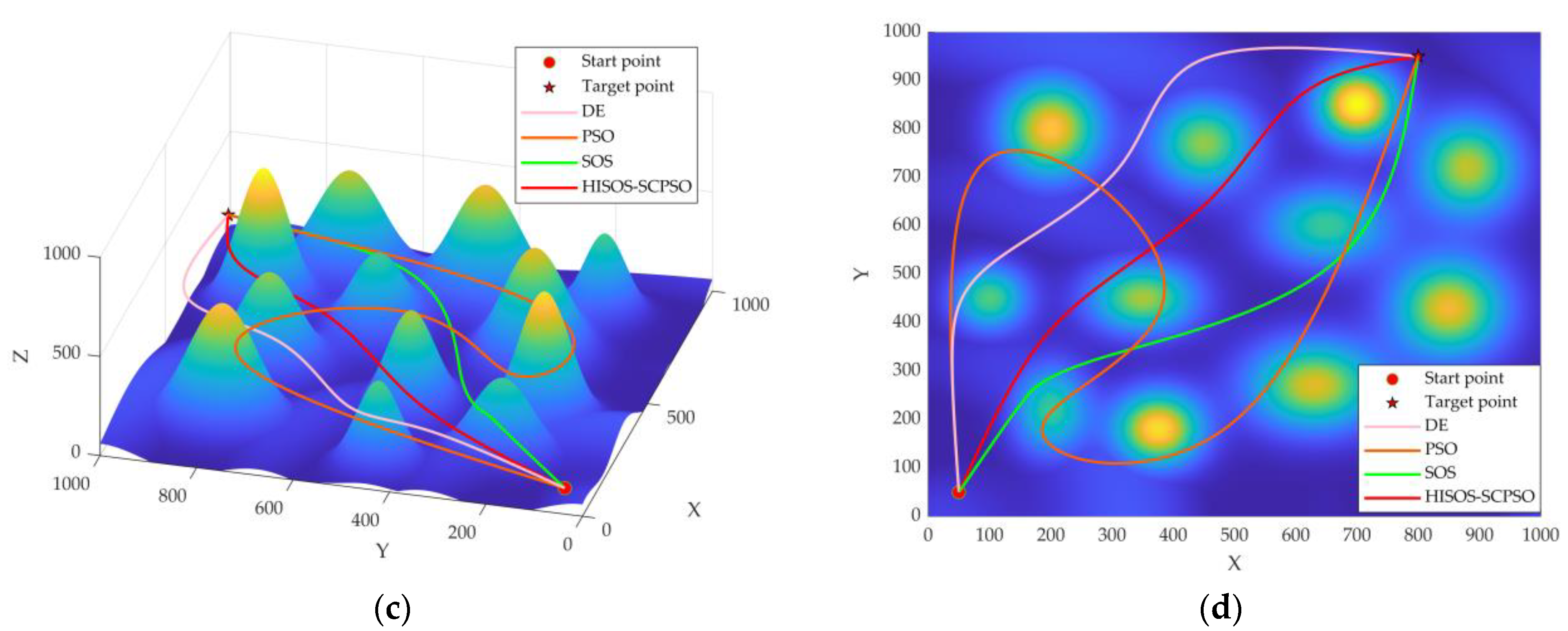
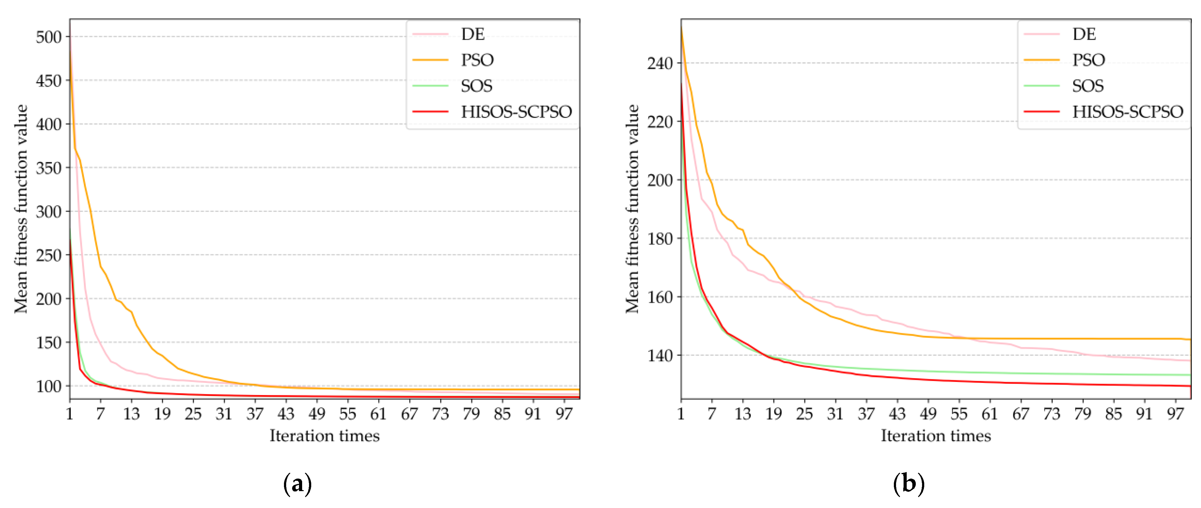
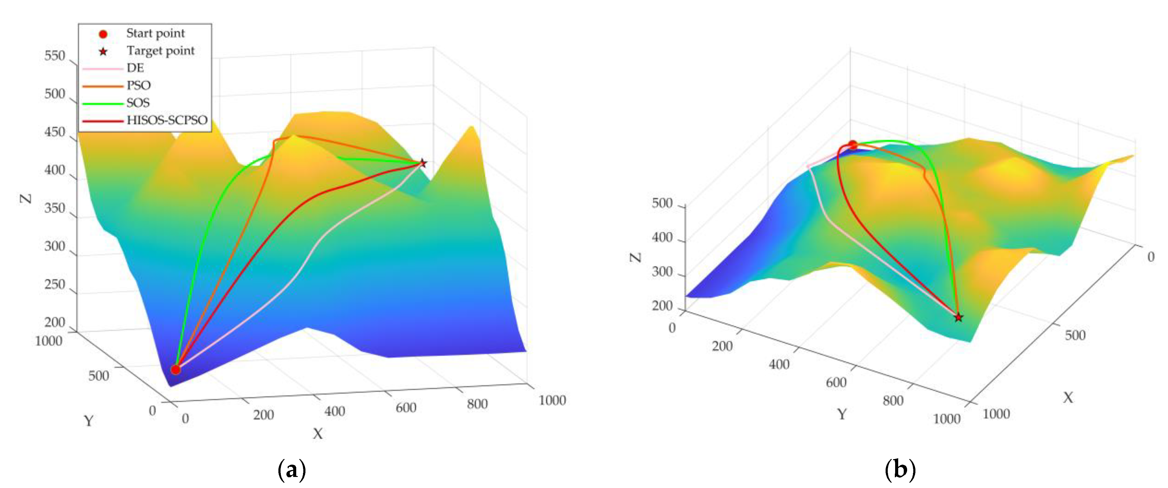
4.1. Evaluation Experiment of 3D Simulated Mountain Terrain

In this section, a comparative experiment is conducted among DE, PSO, SOS, and HISOS-SCPSO for path planning in two 3D simulated mountain terrains. The initial population size NOP is set to NOP = 50, and the population dimension DOP, i.e., the number of path control points, is set to 3 for Case 1 and 4 for Case 2. The maximum number of iterations is set to 100. The dimensions of the two simulated mountain terrains are both 1000 × 1000 × 1000. The drone’s starting and ending coordinates are set to (50, 50, 70) and (800, 950, 320), respectively. Thirty independent experiments are conducted for each of the two cases.

Table 2. Parameter of mountain obstacles.

Case 1
No.	Center Coordinate (x0, y0), Slope (xsl, ysl), and Height hm	No.	Center Coordinate (x0, y0), Slope (xsl, ysl), and Height hm
1	(200, 220), (60, 90), 400	4	(700, 850), (65, 75), 700
2	(250, 750), (80, 100), 600	5	(650, 600), (100, 80), 400
3	(350, 450), (85, 70), 500	6	(650, 250), (150, 90), 500
Case 2
No.	Center Coordinate (x0, y0), Slope (xsl, ysl), and Height hm	No.	Center Coordinate (x0, y0), Slope (xsl, ysl), and Height hm
1	(200, 220), (60, 90), 400	7	(450, 770), (80, 90), 480
2	(200, 800), (80, 100), 600	8	(100, 450), (60, 65), 430
3	(350, 450), (85, 70), 500	9	(880, 720), (80, 100), 520
4	(700, 850), (65, 75), 700	10	(850, 430), (90, 100), 570
5	(650, 600), (100, 80), 400	11	(375, 180), (70, 75), 650
6	(630, 270), (105, 90), 550	12	(840, 180), (65, 60), 410

provides the parameters for the simulated mountain terrain.

Table 3. Performance evaluation metrics for the four algorithms in 3D simulated mountain terrains.

		Fitness Function Value				Mean Runtime(s)
		Best	Worst	Mean	SDV
Case 1	DE	82.1279	84.0127	82.8650	0.5083	0.7037
	PSO	80.9122	96.2893	87.4288	5.4346	0.3907
	SOS	80.3621	82.9940	80.9154	0.4617	1.4419
	HISOS-SCPSO	79.3535	80.9505	80.0901	0.5757	0.7411
Case 2	DE	92.1415	121.3694	110.9071	7.0153	0.8338
	PSO	81.2971	146.9696	120.8978	16.3509	0.4639
	SOS	83.3610	91.3682	85.0827	1.9332	1.6631
	HISOS-SCPSO	80.2106	83.7557	82.5933	1.0675	0.8985

presents the performance evaluation metrics for the four algorithms. It can be observed that in Case 1, although SOS and DE also exhibit good performance, HISOS-SCPSO demonstrates a significant advantage. As the number of mountain obstacles increases, the superiority of HISOS-SCPSO becomes more pronounced. With the exception of the runtime, HISOS-SCPSO outperforms the other methods in all other metrics. Among them, stable standard deviation value (SDV) also shows its strong robustness. While PSO has a lower best value than SOS (in Case 2), its notably elevated mean value and substantial standard deviation value indicate weak robustness. Figure 3 displays the convergence curves of the mean fitness for the four algorithms. It is evident that HISOS-SCPSO exhibits the best convergence performance. Figure 4 illustrates the results of path planning for the four methods. It can be observed that HISOS-SCPSO yields the shortest path distance with the fewest turns in both environments, making it a suitable path for drone flight. SOS and DE follow closely, showing similar performance in Case 1. However, as the environmental complexity increases (in Case 2), SOS outperforms DE significantly. PSO generates the least favorable path, characterized by long distances and unnecessary turns.

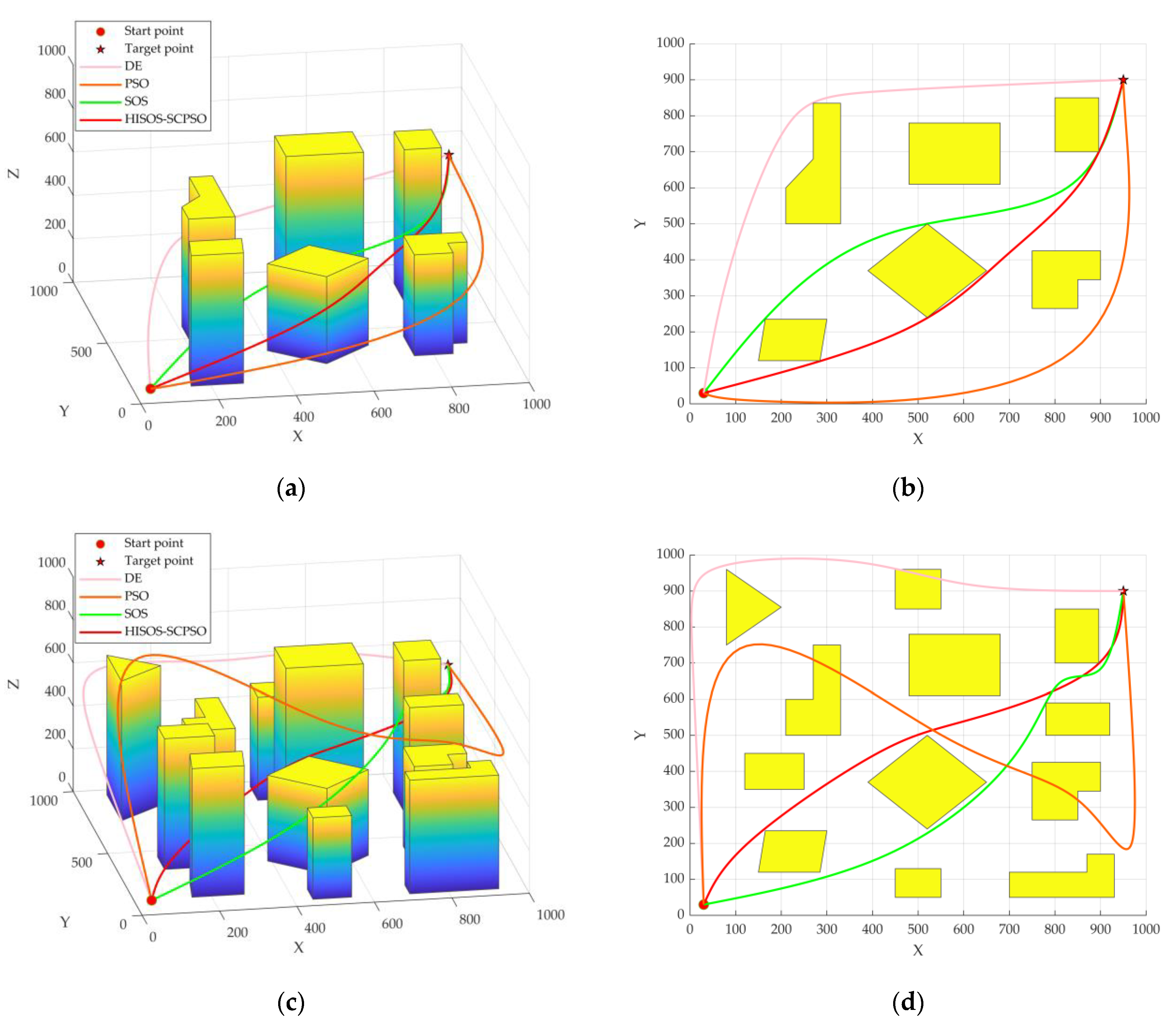
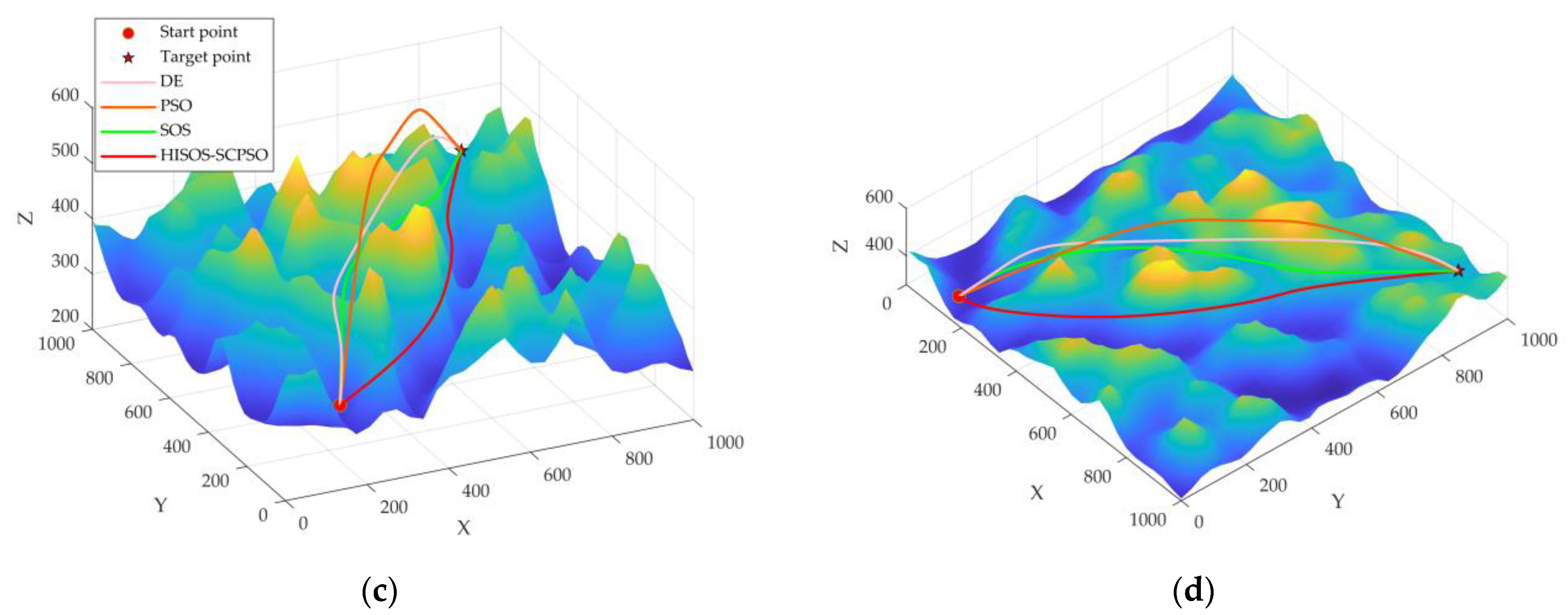
4.2. Evaluation Experiment of 3D Simulated Urban Terrain

In this section, a comparative experiment on path planning using the four methods is conducted in two 3D simulated urban terrains. The algorithm parameters and terrain dimensions remain the same as in the previous section. The drone’s starting and ending coordinates are, respectively, set to (30, 30, 50) and (950, 900, 550). Thirty independent experiments are carried out for each of the two cases.

Table 4. Parameter of urban obstacles.

Case 3
No.	Base Vertex Projection Coordinates (xu, yu) and Height hu	No.	Base Vertex Projection Coordinates (xu, yu) and Height hu
1	(150, 120), (165, 235), (300, 235), (285, 120), 600	4	(520, 240), (390, 370), (520, 500), (650, 370), 400
2	(210, 500), (210, 600), (270, 680), (270, 835), (330, 835), (330, 500), 550	5	(480, 610), (480, 780), (680, 780), (680, 610), 750
3	(750, 265), (750, 425), (900, 425), (900, 345), (850, 345), (850, 260), 464	6	(800, 700), (800, 850), (896, 850), (896, 700), 700
Case 4
No.	Base vertex projection coordinates (xu, yu) and Height hu	No.	Base vertex projection coordinates (xu, yu) and Height hu
1	(150, 120), (165, 235), (300, 235), (285, 120), 600	7	(80, 750), (80, 960), (200, 855), 650
2	(210, 500), (210, 600), (270, 600), (270, 750), (330, 750), (330, 500), 550	8	(450, 50), (450, 130), (550, 130), (550, 50), 380
3	(750, 265), (750, 425), (900, 425), (900, 345), (850, 345), (850, 260), 464	9	(450, 960), (450, 850), (550, 850), (550, 960), 480
4	(520, 240), (390, 370), (520, 500), (650, 370), 400	10	(700, 50), (700, 120), (870, 120), (870, 170), (930, 170), (930, 50), 530
5	(480, 610), (480, 780), (680, 780), (680, 610), 750	11	(120, 350), (120, 450), (250, 450), (250, 350), 610
6	(800, 700), (800, 850), (896, 850), (896, 700), 700	12	(780, 500), (920, 500), (920, 590), (780, 590), 600

presents the parameters for the simulated urban environment, represented by the base vertex projection coordinates and heights of the prisms.

Table 5. Performance evaluation metrics for the four algorithms in 3D simulated urban terrains.

		Fitness Function Value				Mean Runtime(s)
		Best	Worst	Mean	SDV
Case 3	DE	106.8336	116.5442	111.4591	3.2049	12.5984
	PSO	107.1219	123.9882	115.0130	4.3659	7.0010
	SOS	105.6032	114.7277	107.3764	1.6444	29.4895
	HISOS-SCPSO	105.5132	107.2462	105.9946	0.4795	16.0002
Case 4	DE	115.8751	149.7513	133.0243	10.1384	32.2909
	PSO	109.9397	204.0947	162.3170	27.3219	15.8544
	SOS	110.8745	122.7170	114.0504	3.1358	62.9520
	HISOS-SCPSO	106.1866	112.7962	110.5901	2.0190	32.6177

presents a comparison of performance evaluation metrics for DE, PSO, SOS, and HISOS-SCPSO in the experiments involving two simulated urban environments. It can be observed that the mean runtime of the urban environment experiments is significantly higher compared to the mountain terrain experiments. This is due to the discontinuities between the edges of prisms and the ground, which prevent the creation of a continuous elevation model. While SOS also achieves good fitness values, its excessively high time consumption does not align with the urgency of disaster relief scenarios. In contrast, HISOS-SCPSO achieves the best optimization results in only half the time of SOS, and its remarkably low standard deviation values further substantiate its exceptional robustness. Although DE’s runtime is close to that of HISOS-SCPSO, its larger worst and mean values are unsatisfactory, particularly when the complexity of the environment increases. Although PSO has the shortest runtime and the best value is only worse than HISOS-SCPSO in scenarios with increased obstacles, the highest worst, mean, and standard deviation values among the four algorithms indicate its lowest level of robustness. Figure 5 displays the mean fitness convergence curves for the four algorithms. It can be observed that although SOS initially achieves the smallest fitness values, it is quickly surpassed by HISOS-SCPSO. HISOS-SCPSO demonstrates the best convergence speed and optimal fitness. Figure 6 illustrates the path planning results for the four methods. In Case 3, all paths are feasible and smooth; however, HISOS-SCPSO yields the shortest path length and minimal turns. Even as urban obstacles increase in Case 4, HISOS-SCPSO still produces the optimal path. SOS’s path is second, while DE fails to generate a path in the urban center and exhibits longer distances. PSO’s path is the least favorable, with high ascent heights and large turning angles.

4.3. Discussion

After a disaster occurs, every minute, or even every second, of delay can lead to loss of life and further property damage. Therefore, an effective and rapid disaster response mechanism is crucial for minimizing the impact of disasters. Drones play a vital role in disaster response. Drone path planning can guide drones in searching for stranded or missing individuals [41], swiftly reaching disaster zones for preliminary damage assessment [42], and delivering essential supplies like medical supplies and food to disaster areas [43]. It significantly enhances the efficiency of rescue operations. Therefore, drone path planning for disaster response is a crucial field of research. In light of this, a path-planning approach that takes into account drone performance and flight costs is presented in this paper. This method can provide theoretical support for drone path planning in real disaster rescue scenarios.

Since disasters often occur in mountainous and urban areas, two types of simulated 3D terrains are considered in this paper, including mountain and urban. In the future, the terrain feature-aware superresolution model (TfaSR) can be employed to model the disaster area environment [44], making the model more closely resemble real-world conditions. In this paper, a cost function considering flight cost and drone performance is designed as the objective function of the heuristic algorithm. Requirements such as minimizing distance, reducing turns, and minimizing altitude changes are fundamental in drone path planning. In subsequent research, additional factors influencing drone flight could be considered, such as hazard-related costs, which include the threats of emission of electromagnetic waves from collapsed power lines in disaster areas, adverse weather conditions, and variations in airflow.

Currently, there is limited consideration of real 3D environments in existing research. To further validate the effectiveness of the proposed HISOS-SCPSO approach, we conducted additional path-planning experiments using two real 3D mountainous terrains. Given that the southwestern region of China features complex geological conditions due to tectonic plate convergence and is prone to natural disasters, and the karst landform is one of the main terrains in this area [45], two karst terrains in southwestern China are selected as experimental scenarios. The details of the two real terrain datasets are presented in

Table 6. The details of the two real terrain datasets.

	Longitude Range	Latitude Range	Approximate Horizontal Size	Approximate Altitude Range
Case 5	(110.40758 °E, 110.41832 °E)	(25.002104 °N, 25.010851 °N)	1000 m × 1000 m	(219.5 m, 511.43 m)
Case 6	(110.39329 °E, 110.41675 °E)	(25.041794 °N, 25.062988 °N)	2000 m × 2000 m	(277.93 m, 547.93 m)

. These terrains are integrated into a 1000 × 1000 scene, resulting in spatial resolutions of 1m and 2m, respectively. In Case 5, the starting and ending coordinates are set to (20, 20, 240) and (950, 930, 405), respectively. In Case 6, the starting and ending coordinates are (150, 35, 340) and (880, 950, 410), respectively. The population dimension DOP is set to 4, while other algorithm parameters remain consistent with the previous sections. Thirty independent repetitions are conducted for each scenario.

Table 7. Performance evaluation metrics for the four algorithms in 3D real mountain terrains.

		Fitness Function Value				Mean Runtime(s)
		Best	Worst	Mean	SDV
Case 5	DE	89.5573	92.5589	90.3620	0.7807	0.8723
	PSO	88.3561	103.4429	95.7157	4.5199	0.4924
	SOS	87.1556	91.1553	87.5514	0.7445	1.7136
	HISOS-SCPSO	86.8542	87.1995	87.0527	0.0963	0.9508
Case 6	DE	134.5873	142.2764	138.0679	1.7252	0.8624
	PSO	133.3932	156.3994	145.3721	6.0941	0.4879
	SOS	130.7048	136.3455	133.1975	1.6763	1.7055
	HISOS-SCPSO	128.1872	130.8253	129.3975	0.7641	0.9442

presents a comparative analysis of performance evaluation metrics for the four methods in real mountainous terrains. It is evident that, except for the mean runtime, HISOS-SCPSO outperforms the other algorithms in all metrics. In Case 5, while SOS’s best and mean values are competitive with those of HISOS-SCPSO, its mean runtime is nearly twice as long. DE also delivers satisfactory results in this environment. Although PSO has the shortest runtime and better best value than DE, its other metrics are the least favorable among the four methods, although still acceptable for this scenario. As the complexity of the environment increases in Case 6, the performance gaps between the algorithms become more prominent. HISOS-SCPSO remains superior, with its worst value closely approaching the best value achieved by SOS and its lowest standard deviation, highlighting the algorithm’s strong robustness, which means that the optimal result is relatively stable. Figure 7 illustrates the mean fitness convergence curves of the four algorithms in real mountainous terrains. HISOS-SCPSO exhibits the best convergence performance, particularly noticeable as the terrain complexity grows (in Case 6). Figure 8 displays the path planning results of the four methods. In Case 5, although all four methods generated feasible flight paths, HISOS-SCPSO’s path is the most satisfactory: PSO and DE paths lack smoothness; SOS and HISOS-SCPSO paths are smoother, with the latter featuring lower flight altitudes. In the more challenging disaster scenario (in Case 6), HISOS-SCPSO continues to produce the least costly paths; SOS’s path is generally satisfactory; and DE and PSO struggle to plan paths through mountains, resulting in flight paths above the mountains. While this might be safer, it significantly increases the distance traveled, contradicting the urgency of disaster relief efforts. Due to the lower accuracy of existing mapping software in urban areas, comparative experiments on real 3D urban terrains have not been conducted.

In the aforementioned six cases, the mean fitness convergence curve of DE mostly sustains a steep negative slope, indicating a challenge in reaching the optimal value within 100 iterations. Therefore, it is worth studying whether the optimal result of DE is close to HISOS-SCPSO by increasing the maximum number of iterations. The maximum number of iterations for DE and HISOS-SCPSO in Case 2 has been extended to 300 (Case 2’), while the remaining cases have been set to 200 (Case 1’, Case 3’, Case 4’, Case 5’, and Case 6’), with all other algorithm parameters and scenario settings remaining unchanged.

Table 8. Performance evaluation metrics for DE and HISOS-SCPSO in six cases.

		Fitness Function Value
		Best	Worst	Mean	SDV
Case 1’	DE	79.3573	81.4145	79.9616	0.7025
	HISOS-SCPSO	79.2017	79.4372	79.3451	0.0549
Case 2’	DE	80.3101	88.2632	82.8565	2.0621
	HISOS-SCPSO	79.7006	82.9885	81.5449	1.0538
Case 3’	DE	105.6835	113.6417	106.4429	1.4856
	HISOS-SCPSO	105.4441	106.7621	105.8085	0.2671
Case 4’	DE	108.7765	118.4722	113.2985	2.5803
	HISOS-SCPSO	106.1029	112.1629	109.4320	2.0709
Case 5’	DE	86.9648	87.5806	87.2246	0.1510
	HISOS-SCPSO	86.6914	87.3818	86.9389	0.1346
Case 6’	DE	129.3128	134.8471	132.3557	1.1669
	HISOS-SCPSO	127.8550	129.0246	128.4205	0.2861

displays the performance evaluation metrics of DE and HISOS-SCPSO in six scenarios, with their respective running times nearly the same across all six scenarios. Even when the maximum number of iterations is extended to enable DE to converge towards the optimum, the results still do not match the strong performance exhibited by HISOS-SCPSO. In contrast to the previous six cases, DE outperforms SOS in all metrics while maintaining the same runtime. Figure 9 shows the mean fitness convergence curves of DE and HISOS-SCPSO in six cases. HISOS-SCPSO exhibits a significantly swifter convergence rate compared to DE, attaining superior optimal values. Generally, HISOS-SCPSO achieves the optimal value within 100 generations, whereas DE often requires nearly 200 or even 300 generations to achieve the same level of optimization. When considering the time required to reach the optimal value, disregarding the maximum number of iterations, it becomes evident that HISOS-SCPSO accomplishes this objective in less time.

The proposed method in this paper offers at least three notable advantages. First, the practical performance characteristics of drones are considered in our model, ensuring that the generated paths are well-suited for drone flight. Second, considering the urgency of disaster relief, an optimization approach that maintains higher precision and stability while avoiding excessive runtime is proposed. This method is particularly more suitable for path-planning problems with high environmental complexity than other common algorithms. Third, our model exhibits strong adaptability. With elevation information of the task area, our model can rapidly devise optimal paths without requiring additional adjustments. However, our approach also has limitations. For instance, it relies on having complete obstacle information in advance, and any undetected obstacles or sudden events may impact the drones’ survival rate. Moreover, the model does not currently take into account the speed and inertia of the drone, which could affect the drone’s trajectory tracking. Addressing these issues will be a focus of our future work.

5. Conclusions

This paper studies the problem of drone 3D path planning in disaster relief scenarios. Two common disaster scenarios, simulated mountainous terrain and urban environments, are constructed. Flight cost, drone performance, and safety constraints are considered when designing the cost function to ensure that the planned path is flyable. A novel hybrid method named HISOS-SCPSO is proposed to solve the path-planning problem. First, the chaotic logistic map is employed to initialize the population and improve the quality of the initial solution. Then, to achieve rapid computation, the mutualism phase of SOS is improved, followed by integration with SCPSO to enhance the optimization capability. In order to enhance convergence performance, a differential strategy is introduced to the individual cognition part of SCPSO. The novel attenuation functions are proposed, and the global and local optimization capabilities of the algorithm are also improved. Additionally, a population regeneration strategy is designed to enhance algorithm stability. Finally, triple B-spline curves are employed to smooth the flight paths. Experimental results demonstrate that the proposed HISOS-SCPSO achieves superior optimization capabilities within acceptable time consumption. It can plan an available smooth path with the lowest cost for the drone, which has strong competitiveness.

References

1. Liu, J.; Song, Y.; An, S.; Dong, C. How to improve the cooperation mechanism of emergency rescue and optimize the cooperation strategy in China: A tripartite evolutionary game model. Int. J. Environ. Res. Public Health 2022, 19, 1326. [Google Scholar] [CrossRef] [PubMed]
2. Meng, Y.; Xu, J.; He, J.; Tao, S.; Gupta, D.; Moreira, C.; Tiwari, P.; Guo, C. A cluster UAV inspired honeycomb defense system to confront military IoT: A dynamic game approach. Soft Comput. 2021, 27, 1033–1043. [Google Scholar]
3. Tsouros, D.C.; Bibi, S.; Sarigiannidis, P.G. A review on UAV-based applications for precision agriculture. Information 2019, 10, 349. [Google Scholar]
4. Sziroczak, D.; Rohacs, D.; Rohacs, J. Review of using small UAV based meteorological measurements for road weather management. Prog. Aerosp. Sci. 2022, 134, 100859. [Google Scholar]
5. Menouar, H.; Guvenc, I.; Akkaya, K.; Uluagac, A.S.; Kadri, A.; Tuncer, A. UAV-enabled intelligent transportation systems for the smart city: Applications and challenges. IEEE Commun. Mag. 2017, 55, 22–28. [Google Scholar] [CrossRef]
6. Luo, C.; Miao, W.; Ullah, H.; McClean, S.; Parr, G.; Min, G. Unmanned aerial vehicles for disaster management. In Geological Disaster Monitoring Based on Sensor Networks; Springer: Singapore, 2019; pp. 83–107. [Google Scholar]
7. Whitehurst, D.; Joshi, K.; Kochersberger, K.; Weeks, J. Post-flood analysis for damage and restoration assessment using drone imagery. Remote Sens. 2022, 14, 4952. [Google Scholar]
8. Khan, S.I.; Qadir, Z.; Munawar, H.S.; Nayak, S.R.; Budati, A.K.; Verma, K.D.; Prakash, D. UAVs path planning architecture for effective medical emergency response in future networks. Phys. Commun. 2021, 47, 101337. [Google Scholar]
9. Mishra, B.; Garg, D.; Narang, P.; Mishra, V. Drone-surveillance for search and rescue in natural disaster. Comput. Commun. 2020, 156, 1–10. [Google Scholar]
10. Sun, Z.; Yen, G.G.; Wu, J.; Ren, H.; An, H.; Yang, J. Mission planning for energy-efficient passive UAV radar imaging system based on substage division collaborative search. IEEE Trans. Cybern. 2023, 53, 275–288. [Google Scholar] [CrossRef]
11. Ramirez-Atencia, C.; Bello-Orgaz, G.; Camacho, D. Solving complex multi-UAV mission planning problems using multi-objective genetic algorithms. Soft Comput. 2017, 21, 4883–4900. [Google Scholar]
12. Fu, Z.; Yu, J.; Xie, G.; Chen, Y.; Mao, Y. A heuristic evolutionary algorithm of UAV path planning. Wirel. Commun. Mob. Comput. 2018, 2018, 2851964. [Google Scholar]
13. Aggarwal, S.; Kumar, N. Path planning techniques for unmanned aerial vehicles: A review, solutions, and challenges. Comput. Commun. 2020, 149, 270–299. [Google Scholar]
14. Debnath, S.K.; Omar, R.; Latip, N.B.A. A review on energy efficient path planning algorithms for unmanned air vehicles. In Proceedings of the Computational Science and Technology: 5th ICCST 2018, Kota Kinabalu, Malaysia, 29–30 August 2018; pp. 523–532. [Google Scholar]
15. Mokrane, A.; Choukchou Braham, A.; Cherki, B. UAV path planning based on dynamic programming algorithm on photogrammetric DEMs. In Proceedings of the International Conference on Electrical Engineering, Istanbul, Turkey, 25–27 September 2020; pp. 1–5. [Google Scholar]
16. Radmanesh, M.; Kumar, M. Flight formation of UAVs in presence of moving obstacles using fast-dynamic mixed integer linear programming. Aerosp. Sci. Technol. 2016, 50, 149–160. [Google Scholar]
17. Santiago, R.M.C.; De Ocampo, A.L.; Ubando, A.T.; Bandala, A.A.; Dadios, E.P. Path planning for mobile robots using genetic algorithm and probabilistic roadmap. In Proceedings of the IEEE 9th International Conference on Humanoid, Nanotechnology, Information Technology, Communication and Control, Environment and Management, Manila, Philippines, 1–3 December 2017; pp. 1–5. [Google Scholar]
18. Yang, K.; Keat Gan, S.; Sukkarieh, S. A Gaussian process-based RRT planner for the exploration of an unknown and cluttered environment with a UAV. Adv. Robot. 2013, 27, 431–443. [Google Scholar] [CrossRef]
19. Zhou, Y.L.; Huang, N.N. Airport AGV path optimization model based on ant colony algorithm to optimize Dijkstra algorithm in urban systems. Sustain. Comput. Inform. Syst. 2022, 35, 100716. [Google Scholar]
20. Li, X.; Hu, X.; Wang, Z.; Du, Z. Path planning based on combination of improved A-star algorithm and DWA algorithm. In Proceedings of the 2nd International Conference on Artificial Intelligence and Advanced Manufacture, Manchester, UK, 15–17 October 2020; pp. 99–103. [Google Scholar]
21. Wu, J.; Yi, J.; Gao, L.; Li, X. Cooperative path planning of multiple UAVs based on PH curves and harmony search algorithm. In Proceedings of the 2017 IEEE 21st International Conference on Computer Supported Cooperative Work in Design, Wellington, New Zealand, 26–28 April 2017; pp. 540–544. [Google Scholar]
22. He, N.; Su, Y.; Guo, J.; Fan, X.; Liu, Z.; Wang, B. Dynamic path planning of mobile robot based on artificial potential field. In Proceedings of the International Conference on Intelligent Computing and Human-Computer Interaction, Sanya, China, 4–6 December 2020; pp. 259–264. [Google Scholar]
23. Chen, Z.; Xu, B. AGV path planning based on improved artificial potential field method. In Proceedings of the IEEE International Conference on Power Electronics, Computer Applications, Shenyang, China, 22–24 January 2021; pp. 32–37. [Google Scholar]
24. Cheng, M.Y.; Prayogo, D. Symbiotic organisms search: A new metaheuristic optimization algorithm. Comput. Struct. 2014, 139, 98–112. [Google Scholar]
25. Phung, M.D.; Ha, Q.P. Safety-enhanced UAV path planning with spherical vector-based particle swarm optimization. Appl. Soft Comput. 2021, 107, 107376. [Google Scholar]
26. Chai, X.; Zheng, Z.; Xiao, J.; Yan, L.; Qu, B.; Wen, P.; Wang, H.; Zhou, Y.; Sun, H. Multi-strategy fusion differential evolution algorithm for UAV path planning in complex environment. Aerosp. Sci. Technol. 2021, 121, 107287. [Google Scholar]
27. Yu, Z.; Si, Z.; Li, X.; Wang, D.; Song, H. A novel hybrid particle swarm optimization algorithm for path planning of UAVs. IEEE Internet Things J. 2022, 9, 22547–22558. [Google Scholar] [CrossRef]
28. Shao, S.; Peng, Y.; He, C.; Du, Y. Efficient path planning for UAV formation via comprehensively improved particle swarm optimization. ISA Trans. 2020, 97, 415–430. [Google Scholar]
29. Qu, C.; Gai, W.; Zhang, J.; Zhong, M. A novel hybrid grey wolf optimizer algorithm for unmanned aerial vehicle (UAV) path planning. Knowl. Based Syst. 2020, 194, 105530. [Google Scholar]
30. Miao, F.; Zhou, Y.; Luo, Q. A modified symbiotic organisms search algorithm for unmanned combat aerial vehicle route planning problem. J. Oper. Res. Soc. 2019, 70, 21–52. [Google Scholar]
31. Yu, X.; Li, C.; Zhou, J. A constrained differential evolution algorithm to solve UAV path planning in disaster scenarios. Knowl. Based Syst. 2020, 204, 106209. [Google Scholar]
32. Adhikari, D.; Kim, E.; Reza, H. A fuzzy adaptive differential evolution for multi-objective 3D UAV path optimization. In Proceedings of the 2017 IEEE Congress on Evolutionary Computation, San Sebastián, Spain, 5–8 June 2017; pp. 2258–2265. [Google Scholar]
33. Xin, J.; Zhong, J.; Yang, F.; Cui, Y.; Sheng, J. An improved genetic algorithm for path-planning of unmanned surface vehicle. Sensors 2019, 19, 2640. [Google Scholar] [PubMed]
34. Miao, C.; Chen, G.; Yan, C.; Wu, Y. Path planning optimization of indoor mobile robot based on adaptive ant colony algorithm. Comput. Ind. Eng. 2021, 156, 107230. [Google Scholar] [CrossRef]
35. Črepinšek, M.; Liu, S.H.; Mernik, M. Exploration and exploitation in evolutionary algorithms: A survey. ACM Comput. Surv. 2013, 45, 1–33. [Google Scholar]
36. Tsai, C.C.; Huang, H.C.; Chan, C.K. Parallel elite genetic algorithm and its application to global path planning for autonomous robot navigation. IEEE Trans. Ind. Electron. 2011, 58, 4813–4821. [Google Scholar] [CrossRef]
37. Wang, G.G.; Chu, H.E.; Mirjalili, S. Three-dimensional path planning for UCAV using an improved bat algorithm. Aerosp. Sci. Technol. 2016, 49, 231–238. [Google Scholar]
38. Wan, Y.; Zhong, Y.; Ma, A.; Zhang, L. An accurate UAV 3-D path planning method for disaster emergency response based on an improved multiobjective swarm intelligence algorithm. IEEE Trans. Cybern. 2022, 53, 2658–2671. [Google Scholar] [CrossRef]
39. Xiong, T.; Liu, F.; Liu, H.; Ge, J.; Li, H.; Ding, K.; Li, Q. Multi-drone optimal mission assignment and 3D path planning for disaster rescue. Drones 2023, 7, 394. [Google Scholar]
40. Tian, D.; Shi, Z. MPSO: Modified particle swarm optimization and its applications. Swarm Evol. Comput. 2018, 41, 49–68. [Google Scholar]
41. Erdos, D.; Erdos, A.; Watkins, S.E. An experimental UAV system for search and rescue challenge. IEEE Aerosp. Electron. Syst. Mag. 2013, 28, 32–37. [Google Scholar] [CrossRef]
42. Fernandez Galarreta, J.; Kerle, N.; Gerke, M. UAV-based urban structural damage assessment using object-based image analysis and semantic reasoning. Nat. Hazards Earth Syst. Sci. 2015, 15, 1087–1101. [Google Scholar]
43. Liu, H.; Ge, J.; Wang, Y.; Li, J.; Ding, K.; Zhang, Z.; Guo, Z.; Li, W.; Lan, J. Multi-UAV optimal mission assignment and path planning for disaster rescue using adaptive genetic algorithm and improved artificial bee colony method. Actuators 2022, 11, 4. [Google Scholar]
44. Zhang, Y.; Yu, W.; Zhu, D. Terrain feature-aware deep learning network for digital elevation model superresolution. ISPRS J. Photogramm. Remote Sens. 2022, 189, 143–162. [Google Scholar]
45. Zhou, Q.; Luo, Y.; Zhou, X.; Cai, M.; Zhao, C. Response of vegetation to water balance conditions at different time scales across the karst area of southwestern China–a remote sensing approach. Sci. Total Environ. 2018, 645, 460–470. [Google Scholar] [PubMed]
Figure 1. Sketch map of B-spline curve generated by five control points (k = 3). The red curve is a cubic B-spline curve generated by five control points, the five green points represent the control points, and the green line represents the path generated by directly connecting the five control points with straight lines.
Drones 07 00633 g001
Figure 2. The computational flowchart of HISOS-SCPSO.
Drones 07 00633 g002
Figure 3. The convergence curves of the mean fitness for the four algorithms in 3D simulated mountain terrains (a) The convergence curves of the mean fitness of Case 1. (b) The convergence curves of the mean fitness of Case 2.
Drones 07 00633 g003
Figure 4. Visualization results of four algorithms for path planning in 3D simulated mountain terrains (a,b) Visualization results of Case 1. (c,d) Visualization results of Case 2.
Drones 07 00633 g004aDrones 07 00633 g004b
Figure 5. The convergence curves of the mean fitness for the four algorithms in 3D simulated urban terrains (a) The convergence curves of the mean fitness of Case 3. (b) The convergence curves of the mean fitness of Case 4.
Drones 07 00633 g005
Figure 6. Visualization results of four algorithms for path planning in 3D simulated urban terrains (a,b) Visualization results of Case 3. (c,d) Visualization results of Case 4.
Drones 07 00633 g006
Figure 7. The convergence curves of the mean fitness for the four algorithms in 3D real mountain terrains (a) The convergence curves of the mean fitness of Case 5. (b) The convergence curves of the mean fitness of Case 6.
Drones 07 00633 g007
Figure 8. Visualization results of four algorithms for path planning in 3D real mountain terrains (a,b) Visualization results of Case 5. (c,d) Visualization results of Case 6.
Drones 07 00633 g008aDrones 07 00633 g008b
Figure 9. The convergence curves of the mean fitness for DE and HISOS-SCPSO in six cases: (a) The convergence curves of the mean fitness of Case 1’; (b) the convergence curves of the mean fitness of Case 2’; (c) the convergence curves of the mean fitness of Case 3’; (d) the convergence curves of the mean fitness of Case 4’; (e) the convergence curves of the mean fitness of Case 5’; (f) the convergence curves of the mean fitness of Case 6’.
Drones 07 00633 g009