Heterogeneous Drone Small Cells: Optimal 3D Placement for Downlink Power Efficiency and Rate Satisfaction

Abstract

In this paper, we delve into the domain of heterogeneous drone-enabled aerial base stations, each equipped with varying transmit powers, serving as downlink wireless providers for ground users. A central challenge lies in strategically selecting and deploying a subset from the available drone base stations (DBSs) to meet the downlink data rate requirements while minimizing the overall power consumption. To tackle this, we formulate an optimization problem to identify the optimal subset of DBSs, ensuring wireless coverage with an acceptable transmission rate in the downlink path. Moreover, we determine their 3D positions for power consumption optimization. Assuming DBSs operate within the same frequency band, we introduce an innovative, computationally efficient beamforming method to mitigate intercell interference in the downlink. We propose a Kalai–Smorodinsky bargaining solution to establish the optimal beamforming strategy, compensating for interference-related impairments. Our simulation results underscore the efficacy of our solution and offer valuable insights into the performance intricacies of heterogeneous drone-based small-cell networks.

1. Introduction

Recent breakthroughs in unmanned aerial vehicles (UAVs), commonly referred to as drones, have ushered in a new era of extensive drone deployment across diverse application domains, from border control, traffic control, package delivery, and remote sending to disaster management [1,2,3]. These applications span a wide spectrum, encompassing areas like surveillance, shipping and delivery, disaster management, geographical mapping, search and rescue missions, and wireless networking, as noted in Saad et al.’s work [4]. Of particular significance, cellular telecommunications can greatly benefit from the utilization of drone-mounted aerial base stations. This deployment strategy proves instrumental in meeting the coverage and data rate requirements of wireless users, especially in regions with inadequate coverage or severe network congestion, such as high-density urban areas [5,6,7].

The altitude dimension and mobility inherent in drone base stations (DBSs) introduce new dimensions of flexibility that network operators can leverage to enhance the design of airborne cellular systems, as highlighted by Gazestani and Rahimi [8,9]. In contrast to terrestrial base stations, DBSs offer a distinct advantage in establishing line-of-sight (LoS) links with ground stations by adjusting their altitude, as noted in Orsino et al.’s work [10]. Moreover, DBSs exhibit greater adaptability in accommodating the mobility of ground users and environmental fluctuations compared to fixed ground base stations, as emphasized in the study by Electronics [11]. Considering these attributes, including their flexible and on-demand deployment, robust LoS connections, and added design flexibility, DBSs emerge as a promising solution for realizing the vision of ubiquitous connectivity and enhanced network capacity in the next generation of broadband cellular networks, as suggested by Li et al. [12]. Notably, Qualcomm has already unveiled plans to integrate DBSs as a key enabler for pervasive wireless connectivity in the forthcoming fifth-generation (5G) wireless networks [13]. Meanwhile, AT&T’s “Flying Cow” project, also known as Aquila [14], leverages UAV technology to establish an aerial wireless network, delivering ubiquitous Internet access, including in rural and remote areas, at speeds comparable to 4G-LTE.

Developing comprehensive drone-based wireless networks presents distinct technical challenges rooted in the unique characteristics of DBSs, which differ fundamentally from conventional ground base stations:

• The air-to-ground (AtG) wireless channel introduces a novel propagation environment characterized by distinct attributes in contrast to terrestrial channels. Notably, the increased probability of encountering a robust line-of-sight (LoS) component in the received signal, along with the airframe shadowing resulting from the structural design and rotation of the DBSs, represents some of the exceptional features of the AtG channel, as cited in [15].
• The deployment of DBSs occurs naturally within a three-dimensional (3D) space, and the aerial mobility of DBSs necessitates continual dynamic optimization of their 3D positions to enhance overall performance.
• In the design of a drone-based wireless network, it is essential to consider the varying power capabilities of the DBSs. The transmit power range and battery capacity can significantly differ from one DBS to another, depending on the type of drone used. These differences directly influence the quality of service (QoS) delivered by the DBSs to ground users, as outlined in [16].
• Network interference management becomes increasingly complex when deploying DBSs to serve ground users. This is partly attributed to the scenario where ground users may experience strong LoS signals from multiple DBSs, which can considerably degrade the intended signal quality, as discussed in [17]. Additionally, the constrained on-board energy resources of DBSs necessitate the development of efficient and computationally streamlined algorithms to effectively handle interference concerns, as highlighted in [18].

In this paper, we introduce a novel technique for the optimal selection and deployment of a diverse range of DBSs, with the aim of delivering wireless coverage to ground users while simultaneously minimizing the collective transmit power required to meet the downlink data rate requirements. Our contributions in this research can be succinctly summarized as follows:

• We address a repository of heterogeneous DBSs, each with differing transmit power and flight altitude, by jointly determining the optimal resource allocation strategy. This involves selecting a subset of available DBSs and optimizing their 3D placement to minimize the overall transmit power while upholding the specified downlink data rate. Notably, unlike the existing literature, our approach does not assume prior knowledge of the type or quantity of DBSs to be deployed.
• Assuming that the DBSs operate within the same spectrum, we introduce an innovative beamforming method rooted in the Nash bargaining game framework. This approach is designed to mitigate the effects of intercell interference among the DBSs.

To achieve this objective, we break down the optimization problem into two interconnected subproblems, which are solved iteratively. In the first subproblem, assuming that the DBSs are equipped with directional antennas, we tackle an optimization challenge focused on identifying the most suitable subset of DBSs and their corresponding 3D positions. This selection aims to ensure a satisfactory signal-to-noise ratio (SNR) at the ground receivers.

In the second subproblem, taking into account the network topology derived from the first subproblem, we introduce a bargaining game among the interfering DBSs. The goal is to determine the optimal downlink beamforming strategy that enhances the data rates in the interference channel. If the resulting optimal beamforming from this second subproblem meets the required data rate threshold, the iteration concludes. However, if the threshold is not achieved, adjustments to the DBS topology are made to mitigate interference.

This iterative process involves an interplay between the two subproblems, with the outcomes of each subproblem informing the other in subsequent iterations. These calculations are conducted by the control center until the final configurations, including the DBS positions, device associations, and DBS transmit powers, are determined.

The rest of this paper is organized as follows. Section 2 provides an overview of the recent state of the art for the 3D placement of the DBSs. Section 3 presents the system model and describes the air-to-ground channel model as well as the optimal flight altitude of each DBS as a function of their transmit power. The problem formulation is presented in Section 4. The optimal selection and the deployment of the DBSs is investigated in Section 5 while the interference management is addressed in Section 6. The numerical results are provided in Section 7. Finally, Section 8 concludes the paper and discusses the future path of this research.

2. Literature Review

The envisioned opportunities for employing DBSs as a new tier for wireless networking has attracted remarkable recent research activities in the area. A substantial portion of the literature on DBSs is devoted to the AtG channel modeling. For instance, the authors in [19] provided a statistical generic AtG propagation model for low-altitude platform (LAP) systems in which the probability of an LoS channel is derived as a function of the elevation angle. The work in [20] studied the effects of shadowing and pathloss for UAV communications in dense urban environments. As discussed in [21], due to the pathloss and shadowing, the characteristics of the AtG channel depend on the height of the DBSs. A comprehensive survey on the available AtG propagation models can be found in [15].

The 3D deployment of the DBSs is arguably the most influential design consideration in drone-based communications as it directly impacts the coverage, QoS, and life expectancy of the network [6]. The optimal 3D placement of DBSs is a challenging task due to its dependency on the environmental factors (e.g., size and shape of the area), the AtG channel which itself is a function of a DBS’s altitude, and the location and/or distribution of the users on the ground. Consequently, the optimal deployment of DBSs has attracted considerable attention in the recent state of the art.

The optimal flight altitude of a single UAV-BS operating under the Rician fading channel was derived in [22]. The authors in [23] developed an analytical framework to derive the optimal altitude of a single DBS, enabling it to achieve a maximum coverage radius on the ground. This result was extended to the case of two identical DBSs in [24]. The work in [25] investigated the problem of the optimal 3D placement of a symmetric set of DBSs having the same transmit power and altitude. The authors in [26] employed tools from stochastic geometry to analyze the impact of a DBS’s altitude on the sum-rate maximization. In [27], a network on multiple drone base stations that operate on the same frequency band was considered. This paper developed a beamforming solution to maximize the UAV network coverage, noting the intercell interference among the UAVs. In [28], a UAV-enabled small-cell placement optimization problem was investigated in the presence of a terrestrial wireless network to maximize the number of users that can be covered. Furthermore, the authors in [29] proposed a deployment plan for DBSs to minimize the number of drones required for serving ground users within a given area. Similar works can be found in [30,31,32,33,34,35,36]. The authors [37] developed a solution for the 3D positioning of mmWave drone base stations with the objective of maximizing the coverage and minimizing the energy consumption in a scenario where the geographical information of the environment is available.

While these studies address important drone-based communication problems, they mainly limit their discussions to cases in which there exists only a single DBS or multiple identical DBSs with the same capabilities. Moreover, the number of DBSs to be deployed in a given area is assumed to be known in advance. In practice, however, one might have a repository of various types of drones with diverse capabilities in terms of the flight altitude and transmit power. In this context, the exact number and the type of DBSs that need to be deployed depend on the target area and the number of ground users to be served. For instance, having a large set of DBSs, one may need to deploy only a few DBSs in order to cover a small area of interest. Otherwise, the efficiency of resource allocation may drop significantly due to the over-allocation of resources. On the other hand, such an over-allocation of resources may lead to excessive interference between the DBSs, which in turn deteriorates the overall quality of service (QoS). In [38], the authors proposed a novel solution to handle the resource allocation and placement of the DBSs for a rectangular area of interest. However, the work in [38] did not consider the location of the users and the placement was optimized to avoid interference between the DBSs. The assumptions of the related works are summarized in

Table 1. Literature review for DBS placement optimization.

Ref.	Goal	Downlink Rate Satisfaction	DBS Power Optimization	Interference Management	Heterogeneous DBSs	Predetermined Number of DBSs	3D Placement
[23]	Optimal altitude of a single DBS for maximum coverage area	✘	✘	✘	✘	✓	✘
[24]	Optimal distance between two interfering DBSs for best coverage performance	✘	✓	✘	✘	✓	✓
[25]	Optimal placement of symmetric DBSs with same altitude and transmit power to cover a given area	✘	✓	✘	✘	✓	✘
[26]	Quantify the impact of the number and altitude of DBSs on the coverage probability	✘	✓	✘	✘	✘	✓
[28]	Optimal placement of a single DBS to maximize the number of covered ground users	✘	✓	✘	✘	✓	✓
[29]	Optimal 3D placement and the number of required DBSs to cover a set of ground users	✓	✘	✘	✘	✘	✓
[30]	Optimal positioning of a single DBS for users’ throughput maximization	✓	✘	✘	✘	✘	✘
[31]	Optimal 3D placement and movement of DBSs for improving QoE	✓	✘	✘	✓	✓	✓
[32]	Optimal deployment of a single DBS to maximize the sum rate	✓	✓	✘	✘	✓	✓
[33]	Joint optimization of DBSs’ location and intercell interference coordination in LTE-advanced networks	✘	✘	✓	✓	✓	✓
[38]	Joint optimization of DBSs’ location and transmit power for providing maximum coverage area	✘	✓	✘	✓	✘	✓
This work	Three-dimensional location optimization of DBSs for minimizing the total transmit power while satisfying the downlink rate requirement	✓	✓	✓	✓	✘	✓

.

3. System Model

Consider a diverse repository of DBSs, each varying in type based on their transmit power range. For instance, smaller drones may be constrained in their transmit power capabilities, while larger drones, aerostats, and high-altitude platforms can support higher transmit powers. We denote this repository as $\mathcal{D}={D_i}_{i=1}^N$, where N represents the total number of available drones, and $P_i^t$ signifies the transmit power of drone $D_i$. It is important to note that we assume $P_i^t$ falls within the range of $[P_i^{\min },P_i^{\max }]$.

Within a 2D geographical area characterized by low-to-medium ground user mobility, we have a population of K mobile ground users, denoted as $\mathcal{T}={T_j}_{j=1}^K$. Our objective is to efficiently allocate available resources, namely, the DBSs, to provide wireless coverage for ground users while minimizing the overall transmit power. The specific type and quantity of DBSs to deploy are contingent upon the number and spatial distribution of ground users.

Note that our primary objective is to optimize the allocation of DBSs while minimizing the total aggregate power. We do not aim to provide coverage in regions where no users are present. As previously mentioned, one of the key attributes of DBSs is their capability to relocate and adjust their positions to effectively serve ground users. In this study, we focus on determining the optimal placement of DBSs based on a snapshot of user positions. The mobility and trajectory planning of DBSs have been explored in previous research, as detailed in [39,40,41], where the optimal transport theory framework was adopted. Additionally, the work presented in [42] offers a comprehensive overview of methods for optimizing DBS trajectories.

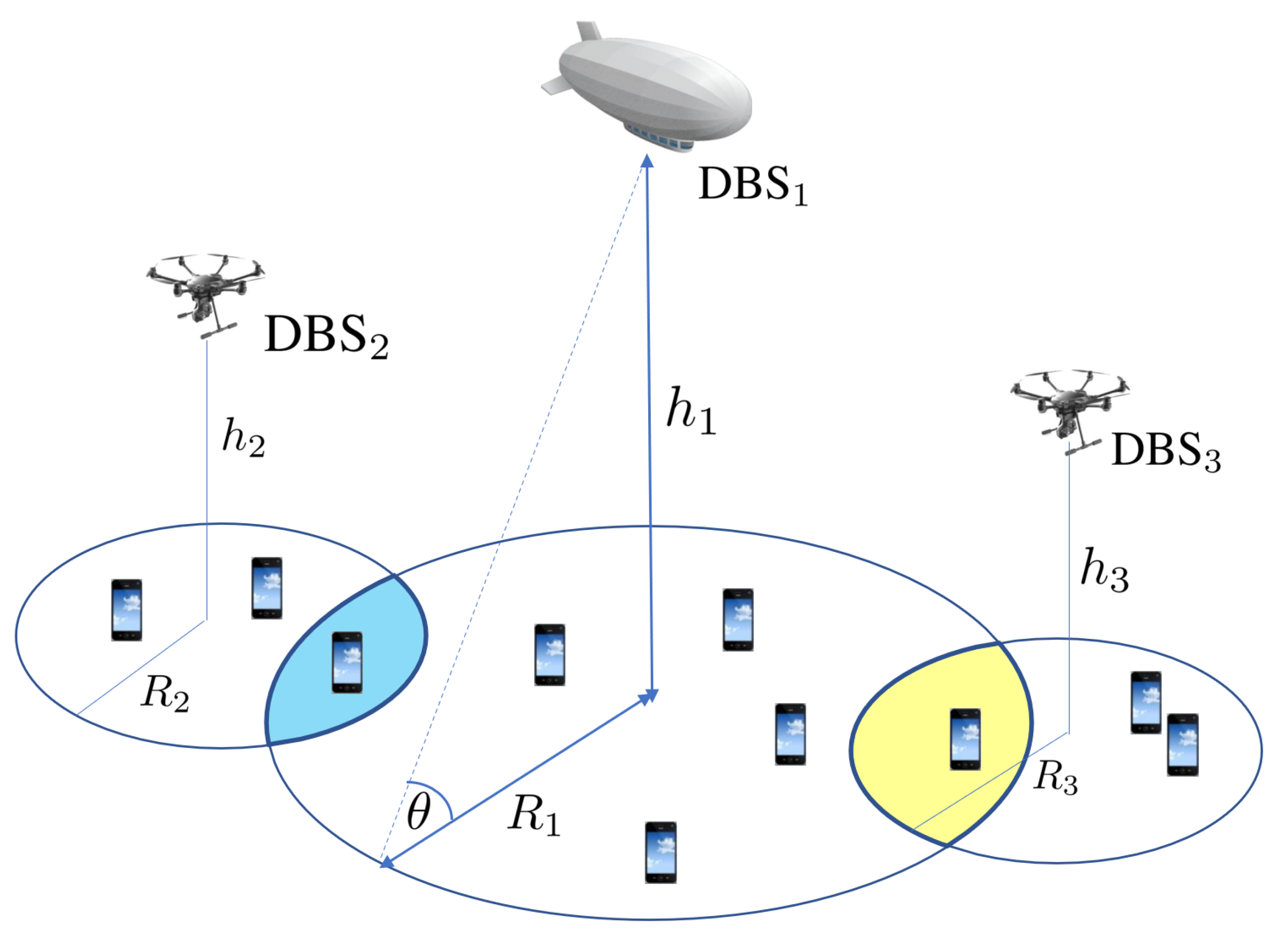
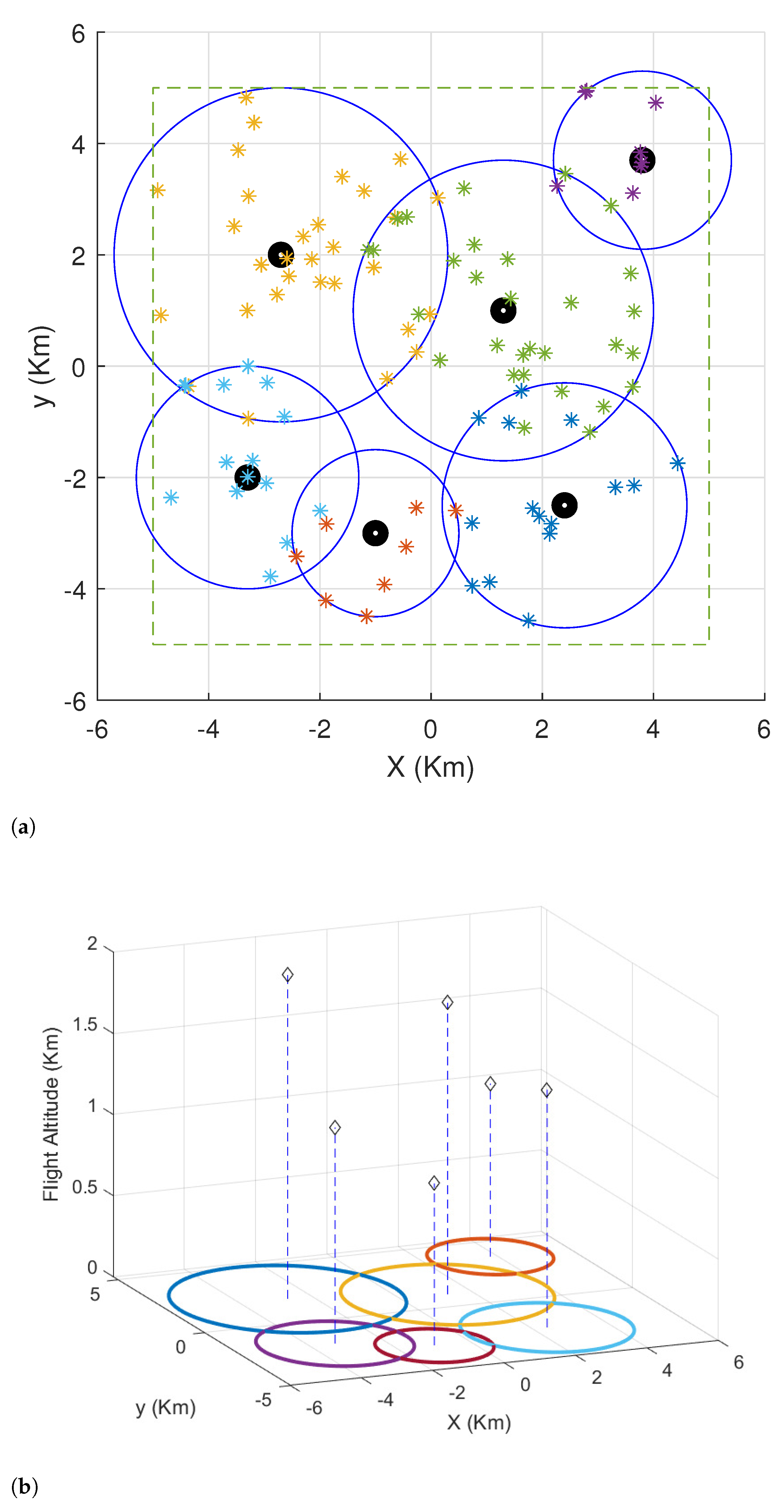
We extend our assumptions to include that the DBSs are interconnected through satellite links or long-range cellular backhaul connections. As illustrated in Figure 1, this depicts our system model. In our study, we treat drones as quasi-stationary Limited Area Platforms (LAPs). It is important to note that while the LAPs are quasi-stationary, the DBSs have the flexibility to hover at varying altitudes to maximize their coverage radius, depending on their transmit power. Furthermore, the DBSs possess the capability to reposition themselves to accommodate the mobility of ground users. In this context, our goal is to optimize the placement of the DBSs, utilizing the drones available in the repository, to deliver wireless coverage with the least energy consumption.

3.1. Air-to-Ground (AtG) Channel Model

The selection of an appropriate air-to-ground (AtG) channel model is a pivotal step in shaping the DBS placement problem. In the literature, numerous empirical and analytical studies have explored AtG channel modeling. However, a substantial portion of researchers in this domain have favored the model introduced in [19] as a reliable and practical representation of the AtG channel. In this section, we provide a concise overview of the AtG channel and its significance in the context of our study.

The radio signal from an LAP base station reaches its destination in accordance with two main propagation groups. The first group corresponds to receiving an LoS signal, while the second group corresponds to receiving a strong NLoS signal due to reflections and diffractions. These groups can be considered separately with different probabilities of occurrence depending on environmental factors, such as building density, height, and elevation angle. In this work, we adopt the model presented in [19] for characterizing the AtG channels for LAP systems.

The AtG channel is represented using Bernoulli random variables for both line-of-sight (LoS) and non-line-of-sight (NLoS) paths. The probabilities of the LoS (${\mathsf{\Psi }}_{\mathrm{LoS}}$) and NLoS (${\mathsf{\Psi }}_{\mathrm{NLoS}}$) transmission between a transmitter and a receiver are as follows:

$$\begin{array}{cc}\hfill {\mathsf{\Psi }}_{\mathrm{LoS}}& ={\left[1+aexp\left(-b\left(\frac{180\theta }{\pi }-a\right)\right)\right]}^{-1},\hfill \end{array}$$

(1)

$$\begin{array}{cc}\hfill {\mathsf{\Psi }}_{\mathrm{NLoS}}& =1-{\mathsf{\Psi }}_{\mathrm{LoS}},\hfill \end{array}$$

(2)

in which the constant parameters $\alpha$ and $\beta$ are determined by the environment, $\theta =arctan(\frac{h}{r})$ is the elevation angle, h is the altitude of the DBS, and r is the radial distance, respectively.

Given the challenge of precisely classifying a channel as either LoS or NLoS, it is customary to consider the spatial expectation of the pathloss over LoS and NLoS links rather than the exact values of the pathloss. The mean pathloss $\mathsf{\Gamma }(\mathrm{dB})$ is given by [19]

$$\mathsf{\Gamma }(\mathrm{dB})=\mathrm{FSPL}+{\eta }_{\mathrm{LoS}}{\mathsf{\Psi }}_{\mathrm{LoS}}+{\eta }_{\mathrm{NLoS}}{\mathsf{\Psi }}_{\mathrm{NLoS}},$$

(3)

where ${\eta }_{\mathrm{LoS}}$ and ${\eta }_{\mathrm{NLoS}}$ denote the excessive pathloss in LoS and NLoS links while $\mathrm{FSPL}=20log\left(\frac{4\pi f_{c}d}{c}\right)$ is the free-space pathloss, in which $f_c$ is the carrier frequency, c is the speed of light, and $d=\sqrt{h^2+r^2}$ is the distance between the DBS and a ground point located at radial distance r.

By substituting ${\mathsf{\Psi }}_{\mathrm{LoS}}$ and ${\mathsf{\Psi }}_{\mathrm{LoS}}$ in (3), we can see that $\mathsf{\Gamma }$ is a function of h and r, implying that the pathloss is a function of the altitude and coverage of the DBS. Indeed, for a given $\mathsf{\Gamma }$, the coverage of a DBS is a function of its altitude. The relationship between $\mathsf{\Gamma }$, h, and r is captured by the following:

$$\mathsf{\Gamma }=20log(d)+\frac{A}{1+aexp\left(-b(\theta -a)\right)}+B,$$

(4)

in which $A={\eta }_{\mathrm{LoS}}-{\eta }_{\mathrm{NLoS}}$ and $B={\eta }_{\mathrm{NLoS}}+20log\left(\frac{4\pi f_c}{c}\right)$.

3.2. The Notion of Coverage and Its Shape

Having defined the expected pathloss in (3), the received signal power at a ground receiver located in radial distance $r_i$ from the ground image of the DBS is given by

$$P^r(\mathrm{dB})=P_i^t(\mathrm{dB})-\mathsf{\Gamma }(\mathrm{dB}).$$

(5)

Definition 1.

We define the service threshold in terms of the minimum allowable received signal power for a successful transmission. Any point in the area is covered if its received signal power is greater than a threshold ϵ,

$$\mathsf{\Gamma }(dB)\le P_i^t(dB)-ϵ.$$

(6)

Proposition 1.

For any given values of the transmit power and flight altitude, the coverage area of a DBS forms a circular disk.

Proof. 

In accordance with Equation (6), for a given transmit power $P_i^t(\mathrm{dB})$, the wireless coverage for a ground point is solely determined by the average pathloss $\mathsf{\Gamma }(\mathrm{dB})$ encountered at that location. However, the pathloss $\mathsf{\Gamma }(\mathrm{dB})$ in (4) relies on the distance between a DBS and the ground station, denoted as $d=\sqrt{h^2+r^2}$, where h signifies the DBS altitude and r represents the horizontal distance to the user. Consequently, for a constant hovering altitude h, the ground users situated at the radial distance r all experience identical pathloss. This implies that the set of points within the 2D area, sharing the same pathloss, forms a circle centered at the ground projection of the DBS. Therefore, the coverage region of a DBS takes the shape of a circular disk.    □

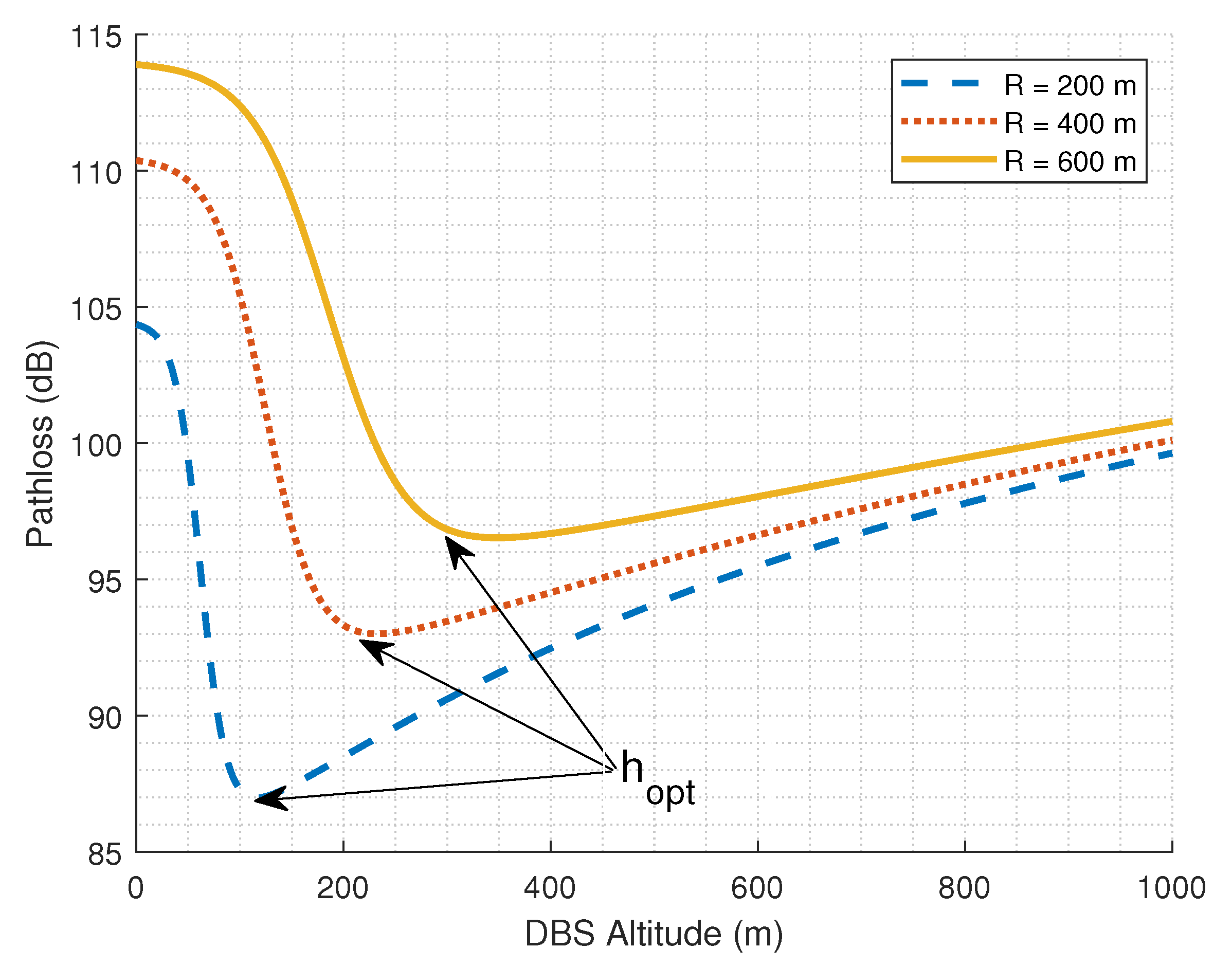
As illustrated in Equation (4), the mean pathloss is implicitly tied to the flight altitude. This relationship is depicted in Figure 2. As evident in the figure, increasing the altitude of a drone-BS initially results in a decrease in pathloss. This decline occurs because at lower altitudes, there is a higher likelihood of non-line-of-sight (NLoS) connections due to reflections from buildings and other obstacles. Additionally, the additional loss incurred in an NLoS connection is greater than that in a line-of-sight (LoS) connection. However, as the altitude increases, the LoS probability rises, subsequently reducing the pathloss. Conversely, the pathloss is also influenced by the distance between the transmitter and receiver. Beyond a certain altitude, this factor becomes dominant, leading to an increase in the pathloss with altitude.

In summary, DBSs can be regarded as a novel tier of access nodes within cellular communication systems, wherein the desired coverage area can be achieved by adjusting the transmit power and/or flight altitude. Moreover, as depicted in Figure 2, for a fixed radial distance, the pathloss exhibits a unimodal relationship with altitude. This observation guides our exploration of the optimal flight altitude for a DBS in the subsequent section.

3.3. Optimal Flight Altitude for a Single DBS

The coverage radius of a DBS with transmit power $P^t$ is defined as the radial distance within which the received signal power at a ground receiver attains the threshold $ϵ$, expressed as

$${R=r|}_{\mathsf{\Gamma }=P^t-ϵ}.$$

(7)

Here, R represents the coverage radius of the DBS. By substituting Equation (4) into the definition above, we obtain

$$20log(d)+\frac{A}{1+aexp\left(-b\left[arctan(\frac{h}{R})-a\right]\right)}+B+ϵ=P^t,$$

(8)

where $A={\eta }_{\mathrm{LoS}}(\mathrm{dB})-{\eta }_{\mathrm{NLoS}}(\mathrm{dB})$ and $B={\eta }_{\mathrm{NLoS}}(\mathrm{dB})+20log(\frac{4\pi f_c}{c})$. Equation (8) demonstrates that for any given value of $P^t$, the radius R implicitly depends on h. As depicted in Figure 2, this function, denoted as ${f(h,r)|}_{P^t=\mathrm{cte}}=0$, is unimodal. Being a unimodal function, ${f(h,r)|}_{P^t=\mathrm{cte}}=0$ possesses a single stationary point, corresponding to the maximum coverage radius. To identify this stationary point, we calculate the partial derivative $\frac{\partial r}{\partial h}=0$, which can be expanded as follows:

$$\frac{h}{R}+\frac{9ln(10)abAexp\left(-b[arctan\left(\frac{h}{R}\right)-a]\right)}{\pi {\left[aexp\left(-b[arctan\left(\frac{h}{R}\right)-a]\right)+1\right]}^2}=0.$$

(9)

The optimal flight altitude along with the corresponding coverage radius can be determined by solving the simultaneous Equations (8) and (9). Unfortunately, there is no closed-form solution for these equations, necessitating the use of numerical methods to find the optimal values of h and R.

It is essential to acknowledge that due to practical constraints on the DBS altitude, we have $h\le h_{\max }$, where $h_{\max }$ represents the maximum allowable flight altitude within the given environment. As depicted in Figure 2, for any specified coverage radius, the DBS transmit power $\mathsf{\Gamma }$ initially decreases as the altitude of the DBS increases, up to a certain point, denoted as $h_{\mathrm{opt}}$, and then begins to rise. Therefore, considering the imposed limitation on the DBS flight altitude, the feasible optimal flight altitude that minimizes the power consumption for a given coverage radius is given by ${\widehat{h}}_{\mathrm{opt}}=min(h_{\mathrm{opt}},h_{\max })$, where ${\widehat{h}}_{\mathrm{opt}}$ is the hovering altitude of the DBS.

4. Problem Formulation

Taking into account the system model depicted in Figure 1, we delve into the combined challenge of selecting and establishing the 3D placement of a diverse set of DBSs, all aimed at delivering wireless coverage to the ground users. Once the positions of all the DBSs have been established, each ground user is assigned to the DBS offering the highest signal-to-interference-plus-noise ratio (SINR). We explore the transmission between DBS i and a ground user situated at the $(x,y)$ coordinates. The attainable rate for the user is expressed as follows:

$${\gamma }_i(x,y)=W_i{log}_2\left(1+\frac{P_i(x,y)/{\mathsf{\Gamma }}_i(x,y)}{N_0+{\sum }_{j\ne i}^N{P}_j(x,y)/{\mathsf{\Gamma }}_j(x,y)}\right),$$

(10)

where $W_i$ is the transmission bandwidth of DBS i, $P_i(x,y)$ is the DBS transmit power to the user, ${\mathsf{\Gamma }}_i(x,y)$ is the average pathloss between DBS i and the user, and $N_0$ is the noise power. Clearly, the number of users covered by the DBS depends on the distribution of users and the location of the DBS.

The minimum transmit power needed to meet the rate requirement $\beta$ for the ground users is given by

$$P_{i,min}(x,y)=\left(2^{\beta /W_i}-1\right){\mathsf{\Gamma }}_i(x,y)\left(N_0+\sum _{j\ne i}^N\frac{P_j(x,y)}{{\mathsf{\Gamma }}_j(x,y)}\right),$$

(11)

which is derived using (10) and $\gamma (x,y)>\beta$.

To achieve the widest coverage in a geographical area encompassing several ground users with known locations while minimizing the overall transmit power, one must address the following inquiries:

• How many DBSs should be selected?
• Which types of DBSs should be chosen?
• For any subset of the DBSs, what is the optimal placement strategy to achieve the minimum aggregate transmit power?
• How should intercell interference be mitigated in scenarios involving overlapping coverage areas?

These questions can be formulated as the following optimization problem:

$$\begin{array}{cc}\hfill & \underset{I_i,(x_i,y_i,h_i)}{\mathrm{minimize}}\sum _{i=1}^N{I}_i{P}_i^t(x_i,y_i),\hfill \\ \hfill & \mathrm{s}.\mathrm{t}.\hfill \end{array}$$

(12)

$$\begin{array}{cc}\hfill & I_i\in \{0,1\},\hfill \end{array}$$

(13)

$$\begin{array}{cc}\hfill & {\gamma }_k(x,y)\ge {\gamma }_0,\hfill \end{array}$$

(14)

$$\begin{array}{cc}\hfill & P_i^t\ge P_{i,min},\hfill \end{array}$$

(15)

$$\begin{array}{cc}\hfill & h_i\le h_i^{\mathrm{opt}},\hfill \end{array}$$

(16)

Here, N represents the total number of available UAVs in the repository. Additionally, $I_i$ serves as an indicator function, taking the value of 1 if DBS $D_i\in \mathcal{D}$ is selected to cover the region and 0 otherwise. This function governs the resource allocation strategy for a given area of interest. Furthermore, ${\gamma }_k(x,y)$ denotes the downlink transmission rate of user k at location $(x,y)$ on the ground, which is determined by the SINR. It is worth noting that users are assigned to the nearest UAV, following the convention in terrestrial networks.

The constraints in (13)–(16) serve distinct roles in the optimization problem. The first constraint in (13) governs the DBS selection scheme, while the second constraint in (14) ensures the ground user quality of service. Additionally, the third constraint in (15) controls the DBS transmit power, and the fourth constraint in (16) relates to the DBS flight altitude. Notably, constraint (16) highlights that within the altitude range $h_i\le h_i^{\mathrm{opt}}$, the transmit power increases monotonically with the coverage radius. This constraint ensures that the transmit power remains a manageable function of the coverage radius and facilitates tractable solutions for the optimization problem in (12).

Methodology

Due to the inherent non-convexity, non-linear constraints and the substantial number of unknowns, the optimization problem articulated in (12) poses a formidable computational challenge. To address this complexity, we decompose the optimization problem outlined in (12) into two sequential subproblems aimed at determining the optimal subset of available DBSs and their respective 3D positions.

In the first subproblem, we temporarily disregard the constraints (14) and (15), which pertain to achievable rate performance, and concentrate on identifying a subset of DBSs that efficiently cover the ground users while minimizing the transmit power. This challenge shares some similarities with the well-studied disk covering problem [43]. However, specific nuances, as elucidated in Section 5, necessitate the development of a custom solution tailored to our problem.

Moving to the second subproblem, after selecting the DBSs and establishing their 3D locations, we introduce a streamlined beamforming technique designed to mitigate co-channel interference within overlapping areas, where the interference-related impairments are most pronounced. In this context, our objective is to achieve the required transmission rate for ground users within the network topology derived from the first subproblem.

It is important to recognize the interdependence between these two subproblems; the solution to the first profoundly impacts the outcome of the second, and vice versa. As a result, we propose a recursive algorithm to address these interwoven challenges. Additionally, we provide a time complexity analysis of the proposed algorithm to gauge its efficiency and scalability.

5. Selection and 3D Placement of the DBSs

In this section, we delve into the combined challenge of resource allocation and the optimal placement of a diverse set of DBSs. Let us consider a scenario with K ground terminals represented as $\mathcal{T}=T_j{j=1}^K$ distributed across a two-dimensional area, with each ground terminal $T_j$ characterized by its coordinates, denoted as $(\tilde{x}j,\tilde{y}j)$. Additionally, we define $(xi,yi,hi)$ as the three-dimensional location of DBS $D_i$ equipped with transmit power $P_i^t$. Our objective is to address the following optimization problem:

$$\begin{array}{cc}\hfill & \underset{I_i,(x_i,y_i,h_i)}{min}\sum _{i=1}^N{I}_i{P}_i^t(x_i,y_i,h_i),\hfill \\ \hfill & \mathrm{s}.\mathrm{t}.\hfill \end{array}$$

(17)

$$\begin{array}{cc}\hfill & I_i\in \{0,1\},\hfill \end{array}$$

(18)

$$\begin{array}{cc}\hfill & P^r({\tilde{x}}_j,{\tilde{y}}_j)\ge ϵ,\forall T_j\in \mathcal{T}\hfill \end{array}$$

(19)

$$\begin{array}{cc}\hfill & h_i=min\{h_{i_{\mathrm{opt}}},h_{\max }\},\hfill \end{array}$$

(20)

$$\begin{array}{cc}\hfill & P_i^t\in [P_{i_{\min }},P_{i_{\max }}],\hfill \end{array}$$

(21)

in which constraint (18) governs the DBS selection strategy, guiding which DBSs are chosen. Simultaneously, constraint (19) guarantees that all the ground users are covered by at least one DBS. It is essential to note that the received power at ground terminal $T_j$ originating from DBS $D_i$ is expressed as $P^r(\tilde{x}j,\tilde{y}j)=P_i^t(xi,yi,h_i)-\mathsf{\Gamma }(d_{ij})$. The mean pathloss $\mathsf{\Gamma }(d_{ij})$ is a function of the distance between $T_j$ and $D_i$, denoted as $d_{ij}=\sqrt{{(x_i-\tilde{x}j)}^2+{(yi-\tilde{x}j)}^2+h{i}^2}$. Additionally, constraint (20) ensures that the DBSs hover at their optimal altitude, while constraint (21) imposes limits on the transmit power of the DBSs.

It is important to emphasize that constraining the flight altitude of the DBSs to $h\in (0,h_{\mathrm{opt}}]$ results in the coverage radius R becoming an increasing function of the transmit power $P^t$. Consequently, given the restriction on DBS flight altitudes within the range $(0,h_{\mathrm{opt}}]$ imposed by constraint (20), our objective shifts to minimizing the DBSs’ coverage radii instead of their transmit power. To achieve this, we undertake the task of minimizing the coverage radii of the DBSs individually, starting with the largest coverage radius. We formulate the following optimization problem aimed at minimizing the largest coverage radius among the deployed DBSs:

$$\begin{array}{cc}\hfill & \underset{(x_i,y_i){|}_{i=1}^N}{min}\underset{({\tilde{x}}_j,{\tilde{y}}_j){|}_{j=1}^K}{max}\underset{(x_i,y_i){|}_{i=1}^N}{min}{I}_i{D}_{ij}\hfill \\ \hfill & \mathrm{s}.\mathrm{t}.\hfill \end{array}$$

(22)

$$\begin{array}{cc}\hfill & I_i\in \{0,1\}\hfill \end{array}$$

(23)

in which $D_{ij}=\sqrt{{(x_i-{\tilde{x}}_j)}^2+{(y_i-{\tilde{x}}_j)}^2}$ is the radial distance between ground terminal $T_j$ and the image of DBS $D_i$ on the two-dimensional Cartesian plane, and the constraint (23) controls the subset selection of the available DBSs.

The optimization problem described in (22) is designed to arrange a set of $M\le N$ coverage disks in a two-dimensional plane with two primary objectives: (1) ensuring that all the ground terminals are encompassed by at least one coverage disk and (2) minimizing the radius of the largest coverage circle. Let us assume that $K_1<K$ ground users are covered by the largest disk. Upon discovering a solution to (22), we have the capability to eliminate the largest coverage disk along with all the ground terminals enclosed within it. Subsequently, we tackle the reduced version of the same problem, involving $M-1$ coverage disks and $K-K_1$ ground terminals. This recursive algorithm iterates until only a single disk remains, the optimal placement of which is then determined to cover the remaining ground terminals with the minimum possible radius. In the subsequent sections, we introduce an efficient algorithm for tackling the optimization problem outlined in (22).

Proposed Algorithm

The problem outlined in (22) bears a resemblance to the well-known planar K-center problem [43]. In the K-center problem, given a set of points in a two-dimensional space, the objective is to arrange a specified number of congruent disks, denoted as M disks, with the centers selected from the given point set. The aim is to cover all the points on the surface while minimizing the radius of these congruent disks. It is important to note that the K-center problem is recognized as NP-hard [44], meaning there is no polynomial-time algorithm to achieve an optimal solution. The literature contains numerous studies addressing various iterations of the K-center problem, many of which focus on the constraint that the disk centers must be chosen from the point set, as is the case with the user locations in our problem [45].

However, the optimization problem presented in (22) possesses distinctive differences from the classic planar K-center problem, necessitating a solution tailored to its specific properties. Firstly, in contrast to the original K-center problem, where disk centers are required to align with predetermined points, the centers of the coverage disks in our scenario can be positioned anywhere on the surface. Secondly, unlike the K-center problem, the number of coverage circles is not known in advance. Lastly, given that the coverage radii of the coverage disks directly correspond to their respective DBS transmit powers, there are constraints limiting both the maximum and minimum coverage radii of these disks. In other words, not all solutions to (22) are feasible, necessitating the identification of a feasible optimal solution.

First, let us introduce some concepts that will be useful later. Consider a subset $\tilde{\mathcal{T}}$ of $\mathcal{T}$, and let $F(\tilde{\mathcal{T}})$ represent the optimal value of the objective function (22) when a single coverage disk is employed to cover all the ground terminals in $\tilde{\mathcal{T}}$. This particular problem is known as the planar 1-center problem and is formulated as a linear programming problem. It can be solved in linear time complexity, specifically in $\mathcal{O}(n)$ time [46]. The value of $F(\tilde{\mathcal{T}})$ is calculated as follows:

$$F(\tilde{\mathcal{T}})=\underset{(x,y)}{min}\underset{({\tilde{x}}_j,{\tilde{y}}_j)\in \tilde{\mathcal{T}}}{max}\sqrt{{(x-{\tilde{x}}_j)}^2+{(y-{\tilde{y}}_j)}^2}$$

(24)

Indeed, $F(\tilde{\mathcal{T}})$ represents the radius of the smallest disk that can cover all the points within the subset $\tilde{\mathcal{T}}$. Additionally, let $X(\tilde{\mathcal{T}})=(x^{\prime }y)$ denote the optimal point for optimization problem (24). It has been demonstrated in [47] that $X(\tilde{\mathcal{T}})$ is unique for any given set of points $\tilde{\mathcal{T}}$.

Next, let $\phi =\{{\tilde{\mathcal{T}}}_1,{\tilde{\mathcal{T}}}_2,\cdots ,{\tilde{\mathcal{T}}}_M\}$ be a partition of $\mathcal{T}$ such that ${\tilde{\mathcal{T}}}_i\bigcap {\tilde{\mathcal{T}}}_j=\varnothing$ and ${\bigcup }_{i=1}^M{\tilde{\mathcal{T}}}_i=\mathcal{T}$. Also, let $F_{\phi }$ be the optimal value of the objective function for partition $\phi$ which is given by

$$F_{\phi }=\left\{F({\tilde{\mathcal{T}}}_1),F({\tilde{\mathcal{T}}}_2),\cdots ,F({\tilde{\mathcal{T}}}_M)\right\},$$

(25)

which is the set of radii of the smallest disks to cover all the points of $\mathcal{T}$ according to partition $\phi$.

We begin the algorithm by selecting M initial center points, denoted as $X^{\left[0\right]}1,X^{\left[0\right]}2,\cdots ,X^{\left[0\right]}M$, for the coverage disks, where $X^{\left[0\right]}i=(x^{\left[0\right]}i,y^{\left[0\right]}i)$. We use the index k to represent the iteration number. At each iteration k, we find the centers $X^{\left[k\right]}1,X^{\left[k\right]}2,\cdots ,X_M^{\left[k\right]}$ by solving the 1-center problem [46] for the corresponding subsets in partition ${\phi }^{\left[k\right]}$. We then assign a set of ground terminals to each center such that each ground terminal is assigned to the closest center. Consequently, the M centers in iteration k define the following partitioning:

$$\begin{array}{c}{\tilde{\mathcal{T}}}_i^{\left[k\right]}=\left\{T_p\right|\sqrt{{(x_i^{\left[k\right]}-x_{T_p})}^2+{(y_i^{\left[k\right]}-y_{T_p})}^2}<\hfill \\ \hfill \hspace{1em}\hspace{1em}\hspace{1em}\hspace{1em}\hspace{1em}\hspace{1em}\hspace{1em}\hspace{1em}\hspace{1em}\hspace{1em}\hspace{1em}\hspace{1em}\sqrt{{(x_j^{\left[k\right]}-x_{T_p})}^2+{(y_j^{\left[k\right]}-y_{T_p})}^2},j=1,2,\cdots ,M\}.\end{array}$$

(26)

Subsequently, we proceed to update the centers of the disks based on the new partitions as described in (26). The new center for each set is determined by solving the 1-center problem for the following set:

$$X_i^{[k+1]}=\left\{\begin{array}{cc}{X}^{*}({\tilde{\mathcal{T}}}_i^{\left[k\right]})\hfill & \mathrm{if}{\tilde{\mathcal{T}}}_i^{\left[k\right]}\ne \varnothing \hfill \\ X_i^{\left[k\right]}\hfill & \mathrm{if}{\tilde{\mathcal{T}}}_i^{\left[k\right]}=\varnothing \hfill \end{array}\right..$$

(27)

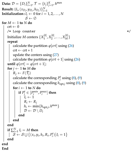
The algorithm iterates until the partitioning no longer changes, denoted as ${\phi }^{\left[k\right]}={\phi }^{[k+1]}$ for a certain iteration k. Upon convergence, this proposed algorithm effectively divides the ground terminals into M subsets. For each subset, it provides the optimal placement of a coverage disk with the minimum radius required to cover all the ground terminals within that specific subset.

Once the coverage radii of the DBSs are determined, along with their corresponding transmit power and flight altitudes, as solved in (8) and (9), it is essential to ensure that the calculated transmit power of all the selected DBSs falls within the permissible range, in accordance with constraint (21). Let $\mathcal{S}$ represent the set of all the feasible solutions. From this set, the optimal solution is chosen based on the minimization of the aggregate transmit power, as it satisfies the constraint. Algorithm 1 outlines the pseudocode of this proposed algorithm.

Algorithm 1: Three-Dimensional Placement of DBSs

It is important to note that certain ground terminals may be covered by more than one coverage disk, leading to significant co-channel interference. In the following section, we introduce a bargaining game formulation designed to model and mitigate this co-channel interference issue for overlapping DBSs.

6. Downlink Beamforming for Interference Management

Facilitating efficient operations of airborne ad hoc systems within the same spectral band poses a significant challenge for drone small cells. Similar to terrestrial wireless cells, intercell interference, a consequence of communication in an interference channel, can degrade the quality of the received signals at ground stations. Numerous algorithms and solutions have been developed to mitigate the impact of co-channel interference in conventional terrestrial networks [48]. However, addressing this issue in airborne small-cell networks presents difficulties due to the limited battery capacity of DBSs. Implementing conventional interference management methods for DBSs is not practical due to the overwhelming computational complexity associated with these battery-limited devices. In this section, we employ the framework of bargaining game theory [49] to introduce a simplified and low-complexity beamforming approach to manage intercell interference.

In the considered scenario, there are M interfering DBSs attempting to transmit data in the downlink to M ground users located within the overlapping area of their respective coverage disks. Assuming that each DBS conducts single-stream transmission and taking into account the assumption of frequency-flat channels, we can express the complex baseband symbols $y_m$ received by the ground users $T_m$ as follows:

$$y_m=h_{mm}^T{w}_m{s}_m+\sum _{l=1,l\ne m}^M{h}_{lm}^T{w}_l{s}_l+e_m,$$

(28)

where the symbols $s_m$, where $1<m<M$, represent the transmitted symbols from DBS $D_m$. The channel vector $h_{lm}$ (with dimensions $K\times 1$) corresponds to the channel between DBS $D_l$ and user $T_m$, while $w_m$ (with dimensions $k\times 1$) is the beamforming vector used by DBS $D_m$. Additionally, $n_m$ denotes the zero-mean additive Gaussian noise with variance ${\sigma }^2$. The maximum transmit power per DBS is normalized to 1, leading to the power constraint on each DBS $D_m$ as follows: $|w_m{|}^2\le 1$ for all $m\in 1,2,\cdots ,M$.

Each DBS $D_m$ aims to optimize its weight vector $w_m$ to maximize the quality of service experienced by its respective ground user. However, there is an inherent interplay between the strategies, as the choice of $w_m$ impacts the choice of $w_l$ for $l\ne m$, and vice versa. Consequently, we must address whether it is possible to implement some form of cooperation among the interfering DBSs to enhance their performance. To explore this, we first evaluate the noncooperative scenario, where DBSs act independently without sharing information. We formulate a noncooperative zero-sum game among the interfering DBSs, with the Nash equilibrium as the expected outcome, as per the game theory principles [50].

6.1. Nash Equilibrium

Consider the noncooperative downlink beamforming game G as the triplet $G=\left\{\mathcal{M},(S_m){{|}_{m\in \mathcal{M}},(u_m)|}_{m\in \mathcal{M}}\right\}$ wherein the following:

• $\mathcal{M}$ is the set of players, i.e., the interfering DBSs;
• $S_m$ is the strategy of DBS $D_m$ which is its choice of weight vector $w_m$ such that $\Vert w_m{\Vert }^2\le 1$;
• $S_{-m}$ is the vector of the strategies of all the DBSs except $D_m$;

  $$S_{-m}=[S_1,\cdots ,S_{m-1},S_{m+1},\cdots ,S_M];$$
• $u_m:[S_m,S_{-m}]\to \mathbb{R}$ is the utility of each DBS $D_m$ which is the rate it achieves at its corresponding ground user.

For a given tuple of beamforming vectors $(w_1,w_2,\cdots ,w_M)$, the received rate at the ground users is given by

$$R_m={log}_2\left(1+\frac{|w_m^T{h}_{mm}{|}^2}{{\sigma }^2+{\sum }_{l=1,l\ne m}^M{\left|w_l^T{h}_{lm}\right|}^2}\right).$$

(29)

We define the utilities of the DBSs as

$$u_m(S_m,S_{-m})=R_m(w_1,w_2,\cdots ,w_M).$$

(30)

As the utilities depend on the strategies of the competing players, we have a noncooperative game among the DBSs. In the absence of coordination among the DBSs, the outcome of the game will generally be the Nash equilibrium. A vector of strategies $(S_1^{\mathrm{NE}},S_2^{\mathrm{NE}},\cdots ,S_M^{\mathrm{NE}})$ is the Nash equilibrium if it satisfies the following condition:

$$u_m(S_m^{\mathrm{NE}},S_{-m}^{\mathrm{NE}})\ge u_m(S_m,S_{-m}^{\mathrm{NE}}),1\le m\le M,$$

(31)

which means that no DBS can unilaterally deviate from its optimal Nash equilibrium strategy without decreasing its own utility. By substituting (29) and (30) in (31) and by performing some algebraic manipulations, we can find the unique equilibrium strategies as

$$w_m^{\mathrm{NE}}=\frac{h_{mm}^{*}}{\left|\right|h_{mm}\left|\right|},1\le m\le M,$$

(32)

where $h_{ij}^{*}$ is the complex conjugate of $h_{ij}$. The equilibrium strategies in (32) correspond to the maximum-ratio transmission beamforming. This conclusion results from the fact that when DBS $D_m$ uses the beamforming vector $w_m^{\mathrm{NE}}$ at the Nash equilibrium, there exists no other vector that can yield a larger rate while satisfying the power constraint $\Vert w_m{\Vert }^2\le 1$.

6.2. Bargaining Solution

The Nash strategies in (32) represent the natural outcome of the considered scenario and it does not necessarily amount to the optimal beamforming strategies for the DBSs. In fact, the inefficiency of the Nash equilibrium solution in (32) is due to the uncoordinated actions of the DBSs. Our goal is to improve on the Nash strategies by allowing some level of cooperation among the DBSs. Note that the DBSs are selfish and try to maximize their own individual rate. Therefore, any sort of cooperation is feasible only if it leads to better utilities, i.e., the downlink transmission rate, for all the involved parties. We show that by a small exchange of information between the interfering DBSs and without any need for a centralized controller, they can coordinate their strategies such that all the involved DBSs benefit from the cooperation.

We define a bargaining game between the interfering DBSs in which the DBSs need to find a point in the achievable rate region which yields a better individual transmission rate for all the interfering DBSs compared to the noncooperative scenario, i.e., the Nash equilibrium rates. Once they agree on a point, the beamforming is optimized accordingly. Let us define the achievable rate region $\overline{\mathcal{R}}$ as

$$\overline{\mathcal{R}}=\underset{w_i,1\le i\le M,\Vert w_i\Vert \le 1}{\cup }(R_1,R_2,\cdots ,R_M),$$

(33)

which is a compact set because the set ${\left\{w_i\right\}}_{i=1}^M$ subject to power constraint $\Vert w_i\Vert \le 1$ is compact and the mapping from ${\left\{w_i\right\}}_{i=1}^M$ to ${\left\{R_i\right\}}_{i=1}^M$ is continuous.

The bargaining game between M DBSs with interfering regions is composed of the following elements:

• The compact and convex set $\mathcal{R}$ of all the possible utilities (i.e., the transmission rates) of the players (i.e., the DBSs). Note that the achievable rate region $\overline{\mathcal{R}}$ defined in (33) is not necessarily a convex set; thus, we consider the convex hull $\mathcal{R}$ of the points in $\overline{\mathcal{R}}$ as the bargaining utility region $\mathcal{R}$. Formally, $\mathcal{R}=\mathrm{Conv}(\overline{\mathcal{R}})$.
• The disagreement point d is the outcome of the bargaining game if the players fail to reach an agreement. Let the disagreement point be the Nash equilibrium rates that the players achieve in the absence of cooperation:

  $$\begin{array}{cc}\hfill d& =\left(R_1,R_2,\cdots ,R_M\right){|}_{w_i=w_i^{\mathrm{NE}},1\le i\le M}\hfill \\ \hfill & =\left(R_1^{\mathrm{NE}},R_2^{\mathrm{NE}},\cdots ,R_M^{\mathrm{NE}}\right).\hfill \end{array}$$

  (34)

Definition 2.

The bargaining solution is a function $f(.)$ that specifies a unique outcome $f(\mathcal{R},d)\in \mathcal{R}$ for every bargaining problem $(\mathcal{R},d)$. Let $f_i(\mathcal{S},d)$ represent the component of player i in the bargaining outcome.

Definition 3.

A bargaining solution $f(\mathcal{R},d)$ is Pareto efficient if there does not exist a point $(R_1,R_2,\cdots ,R_M)\in \mathcal{M}$ such that $R>f(\mathcal{R},d)$ and $R_i>f_i(\mathcal{R},d)$ for some i. Any reasonable bargaining scheme must choose a Pareto efficient outcome because, otherwise, there would exist another outcome that is better for all the players.

There exist several axiomatic definitions for the solution of the bargaining game, such as the Nash bargaining solution (NBS) [50] and the Kalai–Smorodinsky bargaining solution (KSBS) [51]. In this work, we use the KSBS concept because it results in individual fairness which will be explained in the remainder of this section. In the KSBS formulation, given the beamforming bargaining problem $(\mathcal{R},d)$, the rate for the DBSs satisfies the following equation,

$$\frac{R_1-R_1^{\mathrm{NE}}}{R_1^{\max }-R_1^{\mathrm{NE}}}=\cdots =\frac{R_M-R_M^{\mathrm{NE}}}{R_M^{\max }-R_M^{\mathrm{NE}}},$$

(35)

where $R_m^{\mathrm{NE}}$ is the rate of player m at the disagreement point (i.e, the Nash equilibrium), and $R_m^{\max }$ denotes the maximum possible rate for player m. For our problem, achieving $R_m^{\max }$ corresponds to allowing user m to occupy all the available resources, i.e., all the bandwidth in the interference channel, and thus it is easy to determine. Thus, in the Kalai–Smorodinsky bargaining solution (35), every player gets the same fraction of its maximum possible rate, which makes it an attractive approach in situations where one wishes to balance individual fairness with overall system performance. The optimal values of the transmission rate according to the KSBS can be found by solving the following optimization problem:

$$\begin{array}{cc}\hfill & \underset{(w_1,w_2,\cdots ,w_M)}{\mathrm{maximize}}r\hfill \end{array}$$

(36)

$$\begin{array}{cc}\hfill & \mathrm{s}.\mathrm{t}.r=\frac{R_m}{R_m^{\max }},i=1,2,\cdots ,M.\hfill \end{array}$$

(37)

The optimization problem in (36) cannot be solved by the convex optimization techniques due to the fact that the additional equality constraints in (36) are not affine with respect to r and $(w_1,w_2,\cdots ,w_M)$. However, inspecting (35) and (36) reveals that the KSBS corresponds to the intersection of the rate region boundary and the line segment from the origin to the point $(R_1^{\max },\cdots ,R_M^{\max })$. Thus, the optimization problem (36) can effectively be solved by employing the bisection method [52]. The goal of the bisection method is to efficiently search along this line segment until the point of intersection is found.

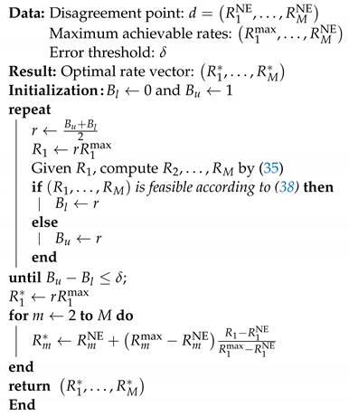
Because $0\le r\le 1$, we set $B_l=0$ and $B_u=1$ as the lower bound and upper bound of r. At each iteration, we bisect the interval between $B_l$ and $B_u$ by the midpoint $\frac{B_l+B_u}{2}$. Then, we check the feasibility test

$$\frac{R_m}{R_m^{\max }}>r^{\prime },m=1,\cdots ,M,$$

(38)

to determine if the current bisection point $r^{\prime }=\frac{R_m}{R_m^{\max }}$ corresponds to an achievable rate pair for some beamforming vector. It is worth noting that due to the fact that $R_m$ is strictly concave with respect to $w_m$, the inequality constraints in (38) are strictly convex, and the test can be performed by standard numerical methods. Once the feasibility is checked, we update the search interval as follows. If the point is feasible, $B_l$ is updated by the current midpoint $\frac{B_l+B_u}{2}$; otherwise, $B_u$ is replaced with $\frac{B_l+B_u}{2}$. This process is repeated until the difference between the lower bound and the upper bound is within the error tolerance $\delta$, which requires at most ${log}_2(\frac{1}{\delta })$ iterations. The pseudocode for the bisection method is shown in Algorithm 2.

Algorithm 2: Bisection Algorithm for KSBS

7. Simulation Results and Discussions

7.1. Simulation Parameters

For our simulation setup, we utilize drone-based communications operating over a 2 GHz carrier frequency, specifically $f_c=2$ GHz, within an urban environment with parameters $a=9.61$ and $b=0.16$ [19]. We assume that a minimum received signal power of $ϵ=-60$ dBm is necessary for a successful transmission. Our repository consists of 12 DBSs, categorized into three types with maximum transmit powers of 35 dBm, 39 dBm, and 43 dBm, each type having four identical DBSs. The objective is to provide wireless coverage for ground users distributed across a 10 km by 10 km area. The key simulation parameters are summarized in

Table 2. Simulation parameters.

Parameter	Value	Parameter	Value
a	9.61	$f_c$	2 GHz
b	0.16	$ϵ$	−60 dBm
${\eta }_{\mathrm{LoS}}$	1 dB	$L_x$	10 Km
${\eta }_{\mathrm{NLoS}}$	20 dB	$L_y$	10 Km
K	10	$\beta$	1 Mbps
${\sigma }_x$	20	N	12
${\sigma }_y$	20	$h^{\max }$	3 Km
$\xi$	0.05	$P_{\max }^t$	$\{35,39,43\}$ dB

for reference.

The ground users are randomly distributed within the area. We consider two distribution models: the uniform distribution and the truncated Gaussian distribution for the users’ locations. Assuming that the x coordinate and y coordinate are independent random variables, these distributions for a rectangular area with dimensions $L_x\times L_y$ are defined as follows:

1. Uniform Distribution: The probability density function (PDF) for the uniform distribution is given by

$$f(x,y)=\frac{1}{L_x·L_y},0\le x\le L_x,0\le y\le L_y$$

2. Truncated Gaussian Distribution: The truncated Gaussian distribution is defined by the PDF:

$$f(x,y)=\left\{\begin{array}{cc}\frac{1}{2\pi {\sigma }_x{\sigma }_y}{e}^{-\frac{1}{2}\left(\frac{{(x-{\mu }_x)}^2}{{\sigma }_x^2}+\frac{{(y-{\mu }_y)}^2}{{\sigma }_y^2}\right)},\hfill & 0\le x\le L_x,0\le y\le L_y\hfill \\ 0,\hfill & \mathrm{otherwise}\hfill \end{array}\right.$$

where ${\mu }_x$ and ${\mu }_y$ are the mean values of the x and y coordinates, respectively, and ${\sigma }_x$ and ${\sigma }_y$ are the corresponding standard deviations. The truncated Gaussian distribution is used for modeling a hotspot area in which the ground users are concentrated around the hotspot center $({\mu }_x,{\mu }_y)$ and their density decreases as they get further away from the center [39].

7.2. Simulation Results

Figure 3 illustrates the optimal resource allocation and 3D placement of the DBSs as well as the user–DBS association for a snapshot of the ground users’ topology. In particular, Figure 3 shows the 2D projection of the DBSs and their corresponding coverage disks. It can be seen that for each coverage disk, there exists at least two ground users on its boundary. Consequently, one cannot shrink any of these coverage disks without leaving some ground users out of the coverage area. In other words, the DBSs’ coverage radii are minimized while providing the required service to the ground users. Figure 3 shows the 3D location of the DBSs. Given the coverage radius of each DBS, its flight altitude has been optimized to minimize the required transmit power. Moreover, it can be seen that only 6 out of the 12 DBSs are deployed in this particular illustrative example. Deploying more DBSs will unavoidably decrease the power efficiency by increasing the intercell interference.

In Figure 4, we present a plot illustrating the average transmit power of the DBSs as a function of the number of ground users. These ground users are uniformly distributed across a 10 Km × 10 area. We compare two scenarios for this analysis: one involving a heterogeneous network comprising all three different types of DBSs and the other involving a homogeneous network with a single type of DBS. The figure reveals an interesting trend. As the number of users increases, the average required transmit power of the DBSs also rises. This outcome is intuitive, as more users necessitate stronger signal transmission to maintain the desired quality of service (QoS). However, an intriguing observation can be made when the number of users exceeds around 100: the change in the optimal DBS placement and their transmit power become less dramatic. This phenomenon can be attributed to the area becoming increasingly saturated, with the network adapting to provide a consistent QoS. Furthermore, it is evident from the plot that as the number of users continues to grow, the DBSs approach their maximum transmit power capacity to fulfill the QoS requirements of the ground users.

Figure 5 presents a comparative analysis of the average transmit power of the DBSs concerning the user density, considering both the optimal DBS placement and Voronoi tessellation. The user distribution follows a truncated Gaussian distribution with the hotspot center situated at the area’s center, precisely at coordinates $({\mu }_x,{\mu }_y)=(0,0)$. To ensure a fair comparison, we employ a methodology where, once the optimal number of DBSs is determined for a given user density, the area is subdivided into equal subareas. A DBS is then placed at the center of each subarea, adhering to the Voronoi cell placement principle. The depicted results unveil a substantial advantage in terms of the average transmit power for the optimal DBS placement approach over the Voronoi counterpart. This difference becomes more pronounced as the user density increases. The reason for this divergence lies in the strategic placement of the DBSs in the optimal approach, where their positions are meticulously chosen to minimize the transmit power based on the user locations. In contrast, the Voronoi approach establishes the DBS locations without accounting for the user spatial distribution. In scenarios with a low user density, where users are more sparsely distributed, the performance of the Voronoi tessellation and the optimal cell boundaries tend to converge. However, as the user density escalates, the superiority of the proposed optimal approach becomes evident, only to reach a point of closer parity once again. This phenomenon arises because in highly dense scenarios, users are spread over a larger area, prompting an increase in the number of DBSs and subareas in the Voronoi tessellation. Consequently, the power efficiency for the Voronoi case is improved in such situations.

Figure 6a presents the optimal number of DBSs necessary to meet the ground users’ coverage requirements while minimizing the average transmit power. This figure reveals a clear trend: the number of DBSs increases in direct proportion to the number of ground users. However, this relationship is not solely determined by user quantity; it is also influenced by their spatial distribution across the area. As depicted in Figure 6a, when dealing with a substantial number of users, the demand for DBSs is relatively lower in a congested hotspot scenario compared to a scenario where users are uniformly distributed over a larger area. Nevertheless, this observation can be deceptive. It is essential to note that achieving coverage with a smaller number of DBSs does not necessarily equate to improved power efficiency. The optimal number of DBSs and power efficiency exhibit significant dependence on the specific user topology. Figure 6b extends this analysis to a homogeneous network with users uniformly distributed. Similar to the previous figure, we observe the monotonically increasing relationship between the number of DBSs and the number of ground users. However, a crucial nuance comes into play: as the power capacity of the DBSs increases, fewer DBSs are required to serve a given number of users. This is primarily due to the direct correlation between the transmit power and the resulting coverage area on the ground. For instance, referring to Figure 6b, when dealing with 140 ground users, the number of required DBSs varies depending on their transmit power capacity. With transmit power capacities of 43 dB, 39 dB, and 35 dB, the corresponding required DBS counts are 5, 6, and 7, respectively. This highlights the intricate interplay between the DBS capabilities, the user distribution, and the optimal allocation of resources to achieve efficient coverage.

Figure 7a unveils the average received data rate experienced by users against varying user quantities under two distinct distribution models. This analysis reveals a noteworthy distinction: the average received data rate is notably lower in hotspot areas when compared to scenarios where users are uniformly distributed across a regular area. This discrepancy stems from the heightened interference generated by closely spaced DBSs within hotspot areas, in contrast to the presumably less interfering DBSs dispersed in more distant, uniformly populated regions. While the latter scenario necessitates a greater number of DBSs, as indicated in Figure 6a, it proves to be more power efficient and affords ground users a higher data rate. Figure 7b extends this evaluation to a homogeneous network configuration of DBSs. It becomes evident that as the number of users increases, the average received data rate declines. In homogeneous networks, DBSs with greater transmit power capabilities can deliver higher data rates to ground users. However, this increased data rate comes at the cost of elevated average transmit power, as illustrated in Figure 4, aligning with our intuitive expectations. Notably, Figure 7b exhibits a notable change in concavity as the number of users rises. This shift is attributed to the heightened likelihood of severe intercell interference as the user count grows, providing insight into the altered concavity in Figure 7b.

8. Conclusions

This paper has introduced an innovative approach to resource allocation and optimal 3D placement in drone-based wireless networks. The method is designed to handle a heterogeneous set of drone base stations (DBSs) and determine the optimal number of DBSs and their respective locations to meet ground users’ rate requirements while minimizing the aggregate transmit power. The inherent complexity of this optimization problem, due to the large number of variables and their interdependencies, has led to its decomposition into two subproblems, solved iteratively for efficiency. In the first subproblem, intercell interference between DBSs is disregarded, and an optimal subset of DBSs, along with their 3D coordinates, is determined based on the received signal-to-noise ratio (SNR) criteria to cover the ground users effectively. In the second subproblem, a Kalai–Smorodinsky bargaining solution is employed to address the intercell interference among the DBSs fairly, improving the users’ data rates, which are directly linked to the signal-to-interference-and-noise ratio (SINR). These subproblems are solved iteratively until convergence is reached. It is noteworthy that the proposed algorithm demands moderate computational resources, making it a practical solution for implementation on DBSs. The results have demonstrated the algorithm’s effectiveness in meeting users’ data rate requirements while minimizing transmit energy consumption.