Sensorless and Coordination-Free Lane Switching on a Drone Road Segment—A Simulation Study

Abstract

Copter-type UAVs (unmanned aerial vehicles) or drones are expected to become more and more popular for deliveries of small goods in urban areas. One strategy to reduce the risks of drone collisions is to constrain their movements to a drone road system as far as possible. In this paper, for reasons of scalability, we assume that path-planning decisions for drones are not made centrally but rather autonomously by each individual drone, based solely on position/speed/heading information received from other drones through WiFi-based communications. We present a system model for moving drones along a straight road segment or tube, in which the tube is partitioned into lanes. We furthermore present a cost-based algorithm by which drones make lane-switching decisions, and evaluate the performance of differently parameterized versions of this algorithm, highlighting some of the involved tradeoffs. Our algorithm and results can serve as a baseline for more advanced algorithms, for example, including more elaborate sensors.

1. Introduction

Unmanned aerial vehicles (UAV) or drones are increasingly becoming an interesting alternative for the delivery of small goods, in particular in densely populated urban environments [1,2,3]. Rotary-wing or copter-type drones are advantageous for this class of applications due to their manoeuvrability, their ability to hover and their vertical take-off and landing capability. Drone-based delivery has important advantages: (i) drones can move in three dimensions and can often take a much more direct route than possible on a street network, reducing the distance to travel and speeding up the delivery of time-critical items; (ii) they are less likely to be hampered by traffic congestion and in turn, do not contribute to the congestion of passenger-carrying vehicles on the ground; (iii) delivery of small goods via drones is potentially more environmentally sustainable, as the mass of a drone to be moved is orders of magnitude lower than the mass of cars or vans (even though the drone additionally has to work against gravity) [4,5,6,7]. We expect that delivery drones will become more autonomous and will be used in increasingly large numbers. At the same time, flying drones present a safety hazard for humans, particularly when a drone loses control and crashes, when two or more drones collide fatally, or when a drone enters an airspace also occupied by manned aircraft (e.g., close to an airport or in the operational area of a rescue helicopter). One approach to manage safety risks is to confine drones to move along pre-planned airspaces most of the time. Therefore, we envisage the introduction of a drone road system  similar to a road network for vehicles, a network of straight cylindrical segments (or tubes) meeting at intersections, which drones can enter and leave either at pre-planned on- and offramps or at arbitrary locations. A drone road network can be partially overlaid with the street network so that a crashing drone hits the ceiling of a car instead of a human.

In this paper, we explore how drones can move along a drone tube such that most of the time they fly at their preferred speed, stay within the tube, and above all avoid collisions with other drones (and subsequent crashes). To cater to a wide variety of drone models and drone operating procedures we make only minimal assumptions about the sensing and communications capabilities of drones. We assume that drones are only equipped with a GPS receiver and a WiFi adapter, and we express this by saying that drones are sensorless. Drones continuously measure their own position and broadcast this and other operational data (e.g., speed) regularly to a local neighbourhood—in other words, our communications model for drones is very similar to the communications model in vehicular networks, which is critically based on the frequent transmission of safety messages [8]. We refer to these periodic transmissions (which are similar in spirit to the WAVE/SAE J2735 protocol’s basic safety messages used in vehicular networking [9]) as beacons. A drone can use beacons received from other drones to estimate their trajectory, identify the risk of upcoming collisions and take corrective actions. Similar to the case of vehicular networks, beacons can get lost through packet collisions and other channel phenomena [10,11,12,13], leading to potentially significant uncertainty about the position and speed of neighbouring drones. These communication-induced uncertainties come on top of other uncertainties, e.g., from noisy GPS receivers or weather conditions [14].

Fundamentally, to move in a tube, drones have to make decisions about their speed and their position relative to the tube, such that they eventually reach their final destination, avoid collisions with other drones or obstacles and do all that at a speed as close as possible to their preferred speed. Drones have to achieve this in the presence of uncertainty about other drones’ positions, resulting from packet losses. In this paper, we report on the design and performance evaluation of a simple, computationally inexpensive, yet flexible autonomous decision-making algorithm for controlling the movements of drones in a drone tube. We make the following contributions:

• We present a system model for a drone tube, in which the space within the tube and outside of it is subdivided into lanes, and in which drones exchange basic position and velocity information through frequent broadcasting of beacons.
• We present a simple, computationally inexpensive, de-centralized and coordination-free decision algorithm, by which drones decide the lane and speed to use, based on information about neighboured drones received through beacons. The algorithm is “greedy”, i.e., it is based on an internal and parameterizable cost model which takes into account both the deviation from the preferred speed and the drone’s position relative to the tube. The algorithm aims to minimize short-term costs. By adjusting the algorithm parameters it becomes possible to choose appropriate tradeoffs between deviations from the preferred speed and temporary movements out of the tube. By “coordination-free”, we mean that drones can make use of the position and speed information gathered from beacons of other drones, but no further data is included in beacons that would allow them to inform (or even actively negotiate with) other drones about any planned movements. Despite its simplicity, the algorithm is parameterizable and can achieve a substantial range of different behaviours. To demonstrate this, we define four noticeably different variants of our algorithm.
• We perform a simulation-based performance analysis of these four variants, reporting results for the average number of drone collisions, average speed, and average distance to the tube when moving out of the tube. The focus of our evaluation is the impact of the underlying communications subsystem on key performance measures such as the number of drone collisions. We, therefore, do not consider other sources of uncertainty, such as GPS noise.

Our results show that: (i) The drone collision rate depends strongly on the density of drones (very likely caused by excessive packet collisions and therefore uncertainty about positions and speeds of neighboured drones), on the beacon sending rate and, broadly, on how “cautious” the algorithm is in its decision-making. (ii) There is a tradeoff between the collision rate and the (reduction of) speed. To avoid frequent slowdowns, drones need to switch lanes to maintain their preferred speed, but this increases the risk of having a collision with other drones.

Our decision algorithm makes only minimal assumptions—it requires no sensors other than GPS and it only relies on simple position and velocity reporting without elaborate coordination. As such, it can serve as a baseline for more advanced algorithms relaxing one or both of these restrictions. (The source code of the simulator is available at https://github.com/zqu14/Drone-lane-switching (accessed on 13 October 2022)).

The remaining paper is structured as follows. In Section 2, we briefly discuss related work. In Section 3, we introduce our system model, including tubes and lanes, drones and drone arrival process, communications and key performance measures. Following this, in Section 4 we introduce the greedy lane-switching (GreedyLS) algorithm, by which drones frequently make decisions on the lane and speed to take over the next short time window. In Section 5, we present and discuss our simulation results and in Section 6 we conclude the paper and discuss potential avenues for future work.

2. Related Work

In this section, we present related studies about path planning and packet loss problems for drones.

2.1. Drone Road Systems

Using drones for deliveries in urban areas is an idea that is gaining traction, ranging from mundane items such as pizzas (https://dronedj.com/2022/01/27/dominos-pizza-drone-delivery-new-zealand/ (accessed on 13 October 2022)) to more critical items such as medications or blood samples [15,16]; see also [17] for a survey drone applications and their communications properties. To simplify air traffic management, drone road systems or drone highways (https://www.altitudeangel.com/news/uk-government-gives-the-green-light-for-worlds-longest-drone-superhighway (accessed on 13 October 2022)) are seen as attractive options and have started to gain traction in the research literature. For example, in [18] a microscopic piecewise-continuous traffic flow model for drones moving in a tube-like “channel” is proposed and analyzed from a stability perspective. In [19], the risk generated by drones moving in a corridor is modelled and an airspace capacity analysis is being carried out, which takes into consideration the collision rate and failure rate of drones. In [20], the modelling of collision risks including risks arising from positional uncertainty is discussed. The required ground infrastructure for urban air mobility and related regulatory aspects are reviewed in [21].

2.2. Dynamic Path Planning for Drones

In our system model, a key challenge for drones is collision avoidance. To achieve that, drones need to continuously detect the position, speed and heading of other drones and plan their own path based on that. Dynamic path planning algorithms [22] address this class of problems. In general, they generate several candidate paths and then choose the optimal one based on a pre-established cost function. In our paper, we benefit from the properties of our system model, which restricts the path decisions a drone can make to a finite (and small) set, limiting computational complexity.

Path conflicts and inconsistency of wireless communication are typical problems for drones when coordinating movements with others. In [23], Zhenyu et al. propose a method to address these issues. The first step is to calculate the probability of a collision by considering a random error vector to simulate the inaccuracy of the position information of other drones, then a Kalman filter [24] is used to predict the state and plan the path. The simulation results show the great effectiveness of the Kalman-filtering-based algorithm to reduce the collision possibility among several drones.

Several papers investigate dynamic path planning in different situations. Ragi and Chong [25] present a partially observable Markov decision process (POMDPs) [26] approach to allow drones to track the positions of others and a target, and avoid collisions with each other. Hu et al. [27] employ reinforcement learning to guide drones while avoiding obstacles. Yu et al. [28] consider target tracking in an urban environment and propose a cooperative path-planning algorithm integrating both aerial and ground-based autonomous vehicles. Xiaolei et al. [29] provide a solution using an improved evolutionary optimization algorithm. It can effectively solve the path planning problem at the cost of high computational complexity.

2.3. Congestion Control in Vehicular Networks

The setup considered in this paper has some similarities to the case of vehicular networks, where vehicles periodically send local broadcasts to inform their neighbourhood about their position, speed and heading. If the underlying wireless technology is based on IEEE 802.11p, then these periodic packets experience both direct and hidden-terminal collisions and this can negatively increase the uncertainty about the position and direction of neighbours and possibly increase collision rates. This is known as the congestion control problem in the context of vehicular ad hoc networks (VANETs) [30,31].

In [32], a simple VANET model is constructed to explore the possible approaches to solve the congestion problem. Their results suggest three key factors: transmit power, packet transmission duration/packet size and packet transmission rate. These can be adapted to reduce the network load and hence control the congestion. There are also many further proposals in the literature to solve the problem by adapting these factors; see [33,34,35,36]. While the effects of congestion in vehicular networks (and by our adoption of related communications technologies also in our drone network) are well understood on a packet level (for example, rates of hidden-terminal and direct collisions), the impact on physical collisions of drones or vehicles is less well studied. This is one of the key problems addressed in this paper.

2.4. Packet Loss in Drone Communications

Packet loss is a crucial problem in drone communications, it can be caused by many reasons. In [37], Fabra et al. investigated several parameters that can affect the packet loss rate between drones. With increasing distance between two drones, the packet loss rate tends to become larger. Furthermore, the degree of change is decided by the on/off status of the engine. When the engine is off, the degree is high. Conversely, the degree becomes low once the engine is turned on. Other parameters such as the remote control proximity and the packet size affect the communication quality between drones only slightly.

In [38], Khalifeh et al. designed experiments to explore the influence of some factors on the packet loss rate between the drones and the ground stations. One interesting finding of this paper is that the height of the drones can have a great impact on the packet loss rate under the utilized ZigBee protocol [39]. The packet loss rate stays at 0% when the height is less than 150 m, and it will rapidly increase to 65% if the height reaches 200 m.

There also exists a rich literature exploring the impact of packet loss. In [40], James et al. examine how the packet loss rate can affect the performances of three drone swarm path planning algorithms [41,42]. The results show that a higher packet loss rate leads to an increased rate of separation violations, thus requiring a larger minimum safety distance to maintain the safety of the drone swarm. In addition, Buonocore et al. [43] have evaluated the impact of some packet loss models on the drone formation control [44]. Results show that even the simplest packet loss models can lead to some abnormal behaviours and collisions under a centralized drone control algorithm [45], and the outcomes become worse when more realistic loss models are used.

3. System Model

In this section, we present our system model, starting with our model for drone tubes and their internal structure, followed by our model for the drones themselves and the drone arrival process, then introducing the communications protocols and channel model used in this work and finally presenting the key performance measures.

3.1. Tube, Lanes and Tiers

For the purposes of this paper, we fix a three-dimensional coordinate system with orthogonal axes, which we simply refer to as the x-, y- and z-axes. We assume that the tube and all lanes (see below) run in parallel to the y-axis, which in turn runs parallel to the surface of the earth. The tube is of finite length L meters. The coordinate origin is placed at one end of the tube such that the y-coordinates of a drone moving in the tube run from 0 (where drones are being injected into the tube) to the length of the tube (where they are removed). 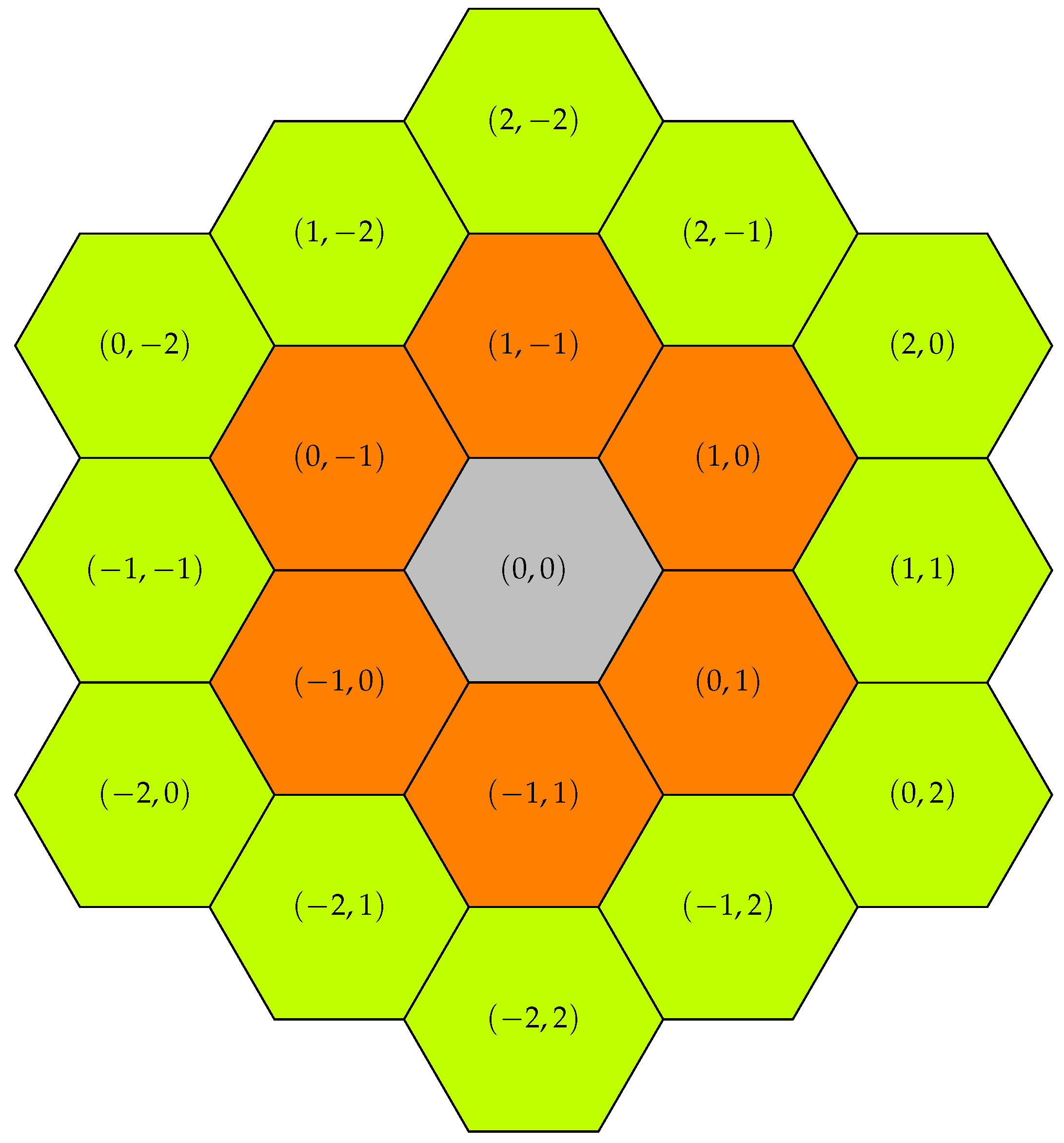The tube itself and the entire space around it is partitioned into lanes, similar to the way a one-way street can be partitioned into lanes. A lane is a hexagonal cylinder wide enough to contain any drone under consideration. A drone will fly in such a way that it is completely within its current lane, with the exception of lane-switching operations—while a drone flies in a lane, its centre point will be on the centre line of the lane. We fix a particular lane to be at the centre of the tube and refer to it as tier-0 or centre lane (shown in grey in Figure 1). Further lanes are packed around the centre lane in the manner indicated in Figure 1, creating a hexagonal tiling. The lanes immediately neighbouring the centre lanes are tier-1 lanes (shown in orange), the lanes immediately neighbouring tier-1 lanes that are not themselves tier-0 or tier-1 lanes are tier-2 lanes (shown in lime), and so on. Note that in this arrangement the centre point of each lane has the same distance as the centre point of each of its six neighboured lanes. As an example, in this paper we assume that tiers 0 and 1 are within the tube, all further tiers are considered to be outside the tube. The GreedyLS algorithm allows drones to move in lanes outside the tube, depending on how its cost model assigns cost to out-of-tube lanes. It is important to point out that our algorithm as such can work with arbitrary numbers of in-tube tiers, including partial tiers.

Across its lifetime, the drone will move in parallel to the y-axis in a positive direction. A drone might change its lane, which corresponds to changes in its x- and z-coordinates. Restricting to these two axes, we can conveniently represent the coordinates of lane centre points and tiers in the following way: if we denote by r the distance between the centre points of neighboured lanes and introduce two basis vectors ${\mathbf{e}}_1$ and ${\mathbf{e}}_2$ in the $x-z$-plane such that ${\mathbf{e}}_1$ points from the centre point of the centre lane (the grey lane in Figure 1, marked as $(0,0)$) to the centre point of the upper right neighbour lane (the orange lane marked as $(1,0)$), and ${\mathbf{e}}_2$ points from the centre point of lane $(0,0)$ to the centre point of the lower right neighbour lane marked as $(0,1)$. With this, the centre points of all lanes can be represented in the form $i·{\mathbf{e}}_1+j·{\mathbf{e}}_2$ with $(i,j)\in {\mathbb{Z}}^2$; compare this with Figure 1. We will frequently refer to a particular lane through these $(i,j)$ integer coordinates. Note that in this setting the centre lane has coordinates $(0,0)$, the lanes on the first tier are given by $(1,0)$, ($-1,0)$, $(0,1)$, $(0,-1)$, $(1,-1)$ and $(-1,1)$, and generally the lanes of the n-th tier are given by:

• Corners: $(n,0)$,$(-n,0)$,$(0,n)$,$(0,-n)$,$(n,-n)$,$(-n,n)$.
• The points $(x,n-x)$ for $x\in \left\{1,\dots ,n-1\right\}$.
• The points $(-x,-(n-x\left)\right)$ for $x\in \left\{1,\dots ,n-1\right\}$.
• The points $(-x,n)$ for $x\in \left\{1,\dots ,n-1\right\}$.
• The points $(x,-n)$ for $x\in \left\{1,\dots ,n-1\right\}$.
• The points $(n,-x)$ for $x\in \left\{1,\dots ,n-1\right\}$.
• The points $(-n,x)$ for $x\in \left\{1,\dots ,n-1\right\}$.

(consider the lanes on tier 2 in Figure 1 as an example). Conversely, to work out to which tier $\tau$ a given point $(i,j)$ belongs, the following formula is helpful:

$$\tau (i,j)=\left\{\begin{array}{ccc}\hfill \mathrm{abs}\left(j\right)& :& i=0\hfill \\ \hfill \mathrm{abs}\left(i\right)& :& j=0,i\ne 0\hfill \\ \hfill \mathrm{abs}\left(i\right)+\mathrm{abs}\left(j\right)& :& sign\left(i\right)=sign\left(j\right),i\ne 0,j\ne 0\hfill \\ \hfill max\left\{\mathrm{abs}\left(i\right),\mathrm{abs}\left(j\right)\right\}& :& \mathrm{otherwise}.\hfill \end{array}\right.$$

(1)

3.2. Drones

We assume all drones to be copter-type, due to their manoeuvrability and their ability to hover and perform vertical take-off and landing. In this paper, we assume that each drone has a preferred speed, which the drone operator can pick as a compromise between required delivery speed and drone energy consumption. The drone will not exceed its preferred speed, but it may travel temporarily at a slower speed when circumstances call for it. We assume that each drone randomly picks its preferred speed from the interval $[20\mathrm{m}/\mathrm{s},30\mathrm{m}/\mathrm{s}]$, independently and from a uniform distribution.

For this paper we have decided to not model the drone dynamics in any detail, we assume that drones can change their speeds instantaneously and that at any given speed lane switching between neighboured lanes takes a constant amount of time $T_{switch}$, which is identical for all drones. Furthermore, for reasons of simplicity we have also decided not to model the size of drones in any detail. Instead, we regard two drones as colliding when the distance of their centre points falls below a threshold of $d_{safety}$ meters. This threshold is also referred to as the safety distance and we assume it to be 0.5 m in this paper. In general, $d_{safety}$ should be smaller than the distance r between centre points of neighboured lanes, so that drones in different lanes do not collide.

Each drone has an accurate GPS receiver, i.e., it can determine its position as well as the current time with sufficiently high accuracy—we do not consider measurement noise. Furthermore, we are not concerned with the power/energy consumption of drones.

3.3. Drone Arrival Process

Drones only arrive at the starting end of the tube ($y=0$) and only leave the system when they collide or reach the other end of the tube. Drones only arrive at intra-tube lanes, and we model arrivals by assigning to each intra-tube lane a separate and stochastically independent random drone arrival process—using random arrivals reflects the independence of drones and the lack of centralized control. In this paper, the arrival process for each intra-tube lane is a Poisson process of rate $\lambda >0$, so that the inter-arrival times of drones are independent and identically distributed with an exponential distribution of parameter $\lambda$.

If we were to insert each arrived drone into its lane unconditionally, we would distort drone collision statistics by a number of unwanted drone collisions, which occur independently of any decision algorithm. The first reason for this is that the inter-arrival times may with a certain probability be so small that the geographical distance between a newly arriving and a previous drone on the same lane is smaller than the safety distance $d_{safety}$. Furthermore, immediately after its arrival, a drone has not yet received any beacon from others, it has no position and speed information about them and therefore cannot take any corrective action such as speeding down.

To deal with this, we distinguish between the arrival and the actual insertion of a drone into its lane, which is subject to certain conditions. If these conditions are not met, an arrived drone is discarded without any further consequences.

Specifically, we check for each generated drone whether it is likely to not experience a collision for at least the first $T_S$ seconds, which we refer to as the insertion safety time. When a drone arrives on lane $l\in {\mathbb{Z}}^2$, it will be inserted when the distance between the new drone and the ahead drone on the same lane is larger than the safety distance $d_{safety}$, and furthermore, one of the following conditions is true:

• Its preferred speed $v_{pref}$ does not exceed the current speed of the drone ahead in the same lane.
• Its preferred speed $v_{pref}$ is larger than the current speed of the drone ahead, but the distance to the drone ahead is large enough for any collision to occur only at a time larger than $T_S$.

Under these assumptions (and in the absence of drones from neighbouring lanes suddenly switching onto lane l) the candidate drone will have at least $T_S$ seconds time to receive beacons and learn where the other drones are. If the conditions are not fulfilled, the generated drone is dropped. We assume this insertion safety time to be $T_S=0.5$ s. The actual GreedyLS algorithm starts running within an inserted drone a little earlier (at 0.4 s) so that it can make adjustments to speed or position before the insertion safety time expires.

3.4. Communications Protocols and Channel Model

We view the requirements for drone communications to be quite similar to the requirements for safety-related communications in vehicular networks [8,9]. We assume that all drones are equipped with a WiFi network adapter [46], operating with similar settings as known from the former IEEE 802.11p amendment. Specifically, they operate in the 5 GHz band over a 10 MHz wide channel, using OFDM with 16-QAM modulation on individual sub-carriers and using a rate-1/2 encoder. These settings result in a 12 Mbps data rate. On the MAC layer, we use the IEEE802.11 EDCA access function, with access class AC_BE, $C{W}_{min}=31$, $C{W}_{max}=1023$ and $AIFS=7$.

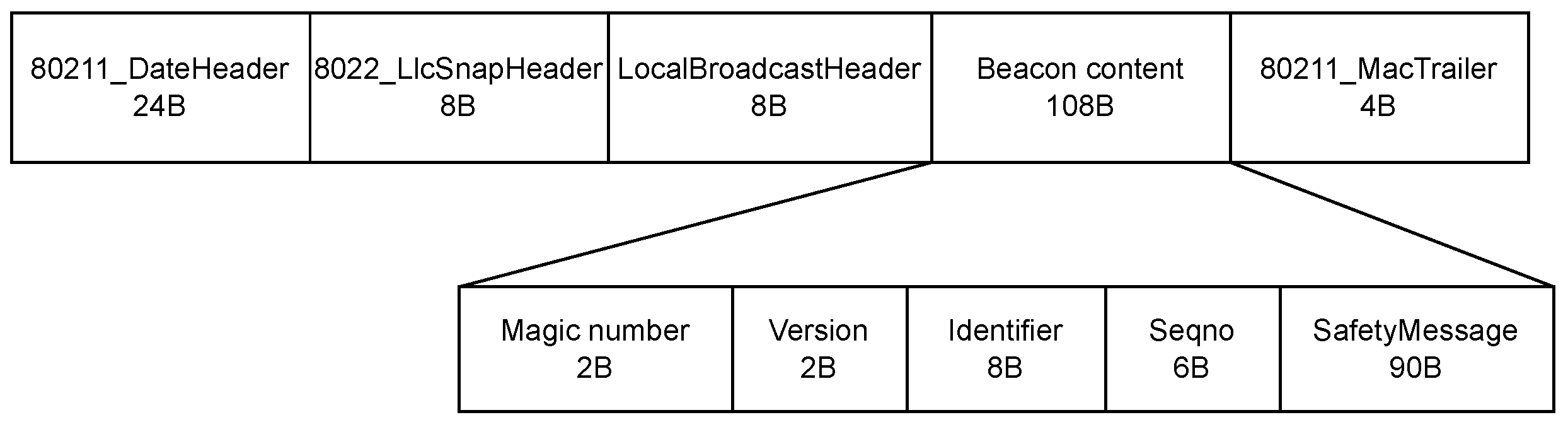
Drones frequently send beacons to their local neighbourhood using a MAC-layer broadcast. We assume that these beacons are the only type of messages that drones send on the considered channel. The beacons contain safety-related information conveying the current position and speed of the sending drone. The beacon size is fixed to a total length of 152 bytes, the beacon contents are shown in Figure 2. In this figure, the “LocalBroadcastHeader” belongs to an enclosing protocol allowing to multiplex different types of local broadcasts, the magic number is a fixed value that helps the receiver to confirm that the beacon contents include a safety message, the version field encodes the version or structure of the safety message being used (this allows to include different types of safety messages), the identifier field is a unique identifier for the sending node, the sequence number is generated by the sending node to allow receivers to estimate packet loss rates and the safety message contains information such as the position and speed of the sending drone. The beacons are being generated almost periodically, with an average rate of $\beta$ beacons per second. The beacons are not generated strictly periodically, but with a jitter of 10% around the average inter-beacon time of 1/$\beta$ seconds. The beacon rate parameter $\beta$ will be varied in our experiments. Furthermore, all drones use the same fixed transmit power $P_t$, which we keep fixed at 5 mW (as an indication of transmission range, this setting leads to a 50% reception rate for our standard beacons at a distance of 119 m).

Each drone stores the information from received beacons in a neighbour table. The neighbour table contains for each currently known neighbour drone the contents of the last correctly received beacon as well as the local timestamp for the time this last beacon was received. The timestamp allows a drone to assess the amount of uncertainty in a neighbours position, but most importantly, the timestamp is critical for the soft-state operation of the neighbour table: the table entries are checked frequently, and when too much time has passed since the last beacon was received, the entry is dropped. The timeout value has been set to ten seconds.

For the wireless channel, we use a simple log-distance channel model with variable path loss exponent $\gamma$ [47], i.e., the received power at distance d meters (for d being at least as large as the reference distance $d_0$, which here we assume to be one meter) is given by

$$P_r\left(d\right)=\frac{P_t}{P{L}_0}·{\left(\frac{d_0}{d}\right)}^{\gamma }$$

(2)

where $P{L}_0$ is the path loss at the reference distance, which we assume to be 40 dB. This is a reasonable model when drones operate sufficiently far away from any reflecting surfaces and any shadowing from the drone’s body is ignored. We have used a path loss exponent of $\gamma =2.5$ for our simulations. Furthermore, we assume that there is no external interference.

3.5. Key Performance Measures and Problem Formulation

We use three key performance measures to assess the algorithms proposed in this paper. They are:

• The average number of collisions per kilometre, where the average is taken over a number of replications for a given set of parameters.
• The average speed of drones, taken over all inserted drones within a replication (sampled regularly) and all replications for a given set of parameters. Note that, due to the fact that preferred speeds are drawn uniformly from $[20\mathrm{m}/\mathrm{s},30\mathrm{m}/\mathrm{s}]$ and that drones are not allowed to go above their preferred speed, the average speed will not exceed 25 m/s, and will often be below that.
• Average out-of-tube tier of drones, taken over all inserted drones within a replication (sampled regularly) and all replications for a given set of parameters. In this statistic the in-tube lanes will enter with a contribution of zero, the second tier (the first tier out of the tube) will enter with a contribution of one, and so forth.

In our system model the key control knobs for a drone are the lane and the speed to use, and it decides these dynamically based on the current neighbourhood. For real deployments, a decision algorithm for speed and lane generally will attempt to maximize both the average speed and the drone density, subject to constraints on the average number of collisions and occupancy of out-of-tube lanes. Instead of maximizing the average speed, one might be interested in minimizing the maximum deviation from the preferred speed. However, as the focus of this paper is more on exploring the tradeoffs achievable with one particular algorithm, in our experiments we vary the drone density (or drone generation rate) and obtain results for the number of collisions, the average speed and the lane occupancy for different parameterizations or variants of the algorithm, so that we can understand their tradeoffs.

3.6. Summary of All Fixed Parameters

The key fixed parameters for this paper are summarized in

Table 1. Key parameters.

Parameter	Explanation	Value
Tube parameters
r	Distance of neighbour lane centre points	1 m
L	Tube length	$1\mathrm{km}$
Drone and drone arrival parameters
$d_{safety}$	Minimal safety distance	0.5 m
	Preferred speed distribution	$U[20\mathrm{m}/\mathrm{s},30\mathrm{m}/\mathrm{s}]$
$T_{switch}$	Time required for switching to a neighbouring lane	1 s
$\lambda$	Drone arrival rate to an in-tube lane	$\lambda \in \left\{0.1,0.3,\dots ,1.5\right\}$
$T_S$	Insertion safety time	0.5 s
Communications and channel parameters
	Beacon length (total)	152 B
	PHY data rate	12 Mbps
$\beta$	Beaconing rate	$\beta \in \left\{10\mathrm{Hz},20\mathrm{Hz}\right\}$
$P_t$	Transmit power	5 mW
$P{L}_0$	Path loss at reference distance	40 dB
$\gamma$	Path loss exponent	2.5
	Neighbour table timeout	10 s

.

Our parameter settings are not in all cases completely realistic (e.g., lanes would normally be wider than one meter), and we have also chosen to ignore the noise in parameters such as the GPS position readings. This is for two reasons. First, our parameters have been chosen to achieve a higher rate of collisions, helping to more clearly highlight the performance difference between the considered algorithms and displaying their relative performance merits, and also avoiding rare-event simulation. Secondly, by restricting the position uncertainty in the system to the effects of packet losses, we can clearly investigate and display their impact, avoiding confounding the effects of packet losses with other sources of uncertainty.

4. The Greedy Lane-Switching (GreedyLS) Algorithm

In this section, we first give a generic description of the greedy lane-switching (or GreedyLS) decision algorithm, followed by presenting a number of algorithm variants with specific choices for the cost parameters, expressing different tradeoffs between speed and position cost.

4.1. Algorithm Description

We now describe the decision algorithm by which each drone decides the lane and speed to use in the next few seconds. The decision algorithm runs periodically. The (average) period needs to be significantly larger than the time required to switch to a neighboured lane or to change the speed to a given setting. This allows us to treat lane switching and speeding up/down as elementary actions and avoids the need to maintain state information that would be necessary when these actions took multiple periods. We also refer to the (average) period as the unit time.

Our decision algorithm is “stateless”. i.e., a decision is always made only based on current circumstances, not based on previously stored state information (other than the contents of the neighbour table), and it is “greedy” in that it seeks to minimize costs in the short-term, over only the next unit time. The algorithm does not allow drones to operate at speeds higher than their preferred speed, only at lower speeds.

The cost model used for the algorithm employs two different types of cost. The drone knows for every tier $\tau \in \left\{0,1,2,\dots \right\}$ the position cost for spending one unit of time at tier $\tau$, we refer to this unit position cost as $c_p\left(\tau \right)$. The mapping $c_p(·)$ is known and identical for all drones. Similarly, for a given speed v and preferred speed $v_{pref}$ there is a mapping $c_s(·)$ which gives the speed cost $c_s(v,v_{pref})$ of operating at speed v for one unit time when the preferred speed is $v_{pref}$.

The GreedyLS algorithm runs on each drone separately and independently. It has the following inputs:

• The current lane $l\in {\mathbb{Z}}^2$ and tier $\tau =\tau \left(l\right)$ (cf., Equation (1)).
• The speed $v_{ahead}$ of the drone ahead in the same lane l. If there is no (known) ahead drone, then $v_{ahead}=\infty$.
• The distance $d_{ahead}$ to the ahead drone in the same lane l. If there is no (known) ahead drone, then $d_{ahead}=\infty$.
• For all available neighbour lanes:

  -

  Their lane number $l_i\in {\mathbb{Z}}^2$ and tier ${\tau }_i=\tau \left(l_i\right)$.

  -

  The distance $d_{i,ahead}$ to the closest drone ahead of us (taken in the y-coordinate only) and having a y-coordinate at least as large as our own in lane $l_i$, and its speed $v_{i,ahead}$.

  -

  The distance $d_{i,behind}$ to the closest drone behind us in lane $l_i$, and its speed $v_{i,behind}$.

  If we want to also consider “concurrent collisions” (see below) then the neighbour lane information above must be extended to include all lanes in the first two tiers around the current lane.

Note that $d_{i,ahead}$, $d_{i,behind}$, $v_{i,ahead}$ and $v_{i,behind}$ are all inferred from the neighbour table.

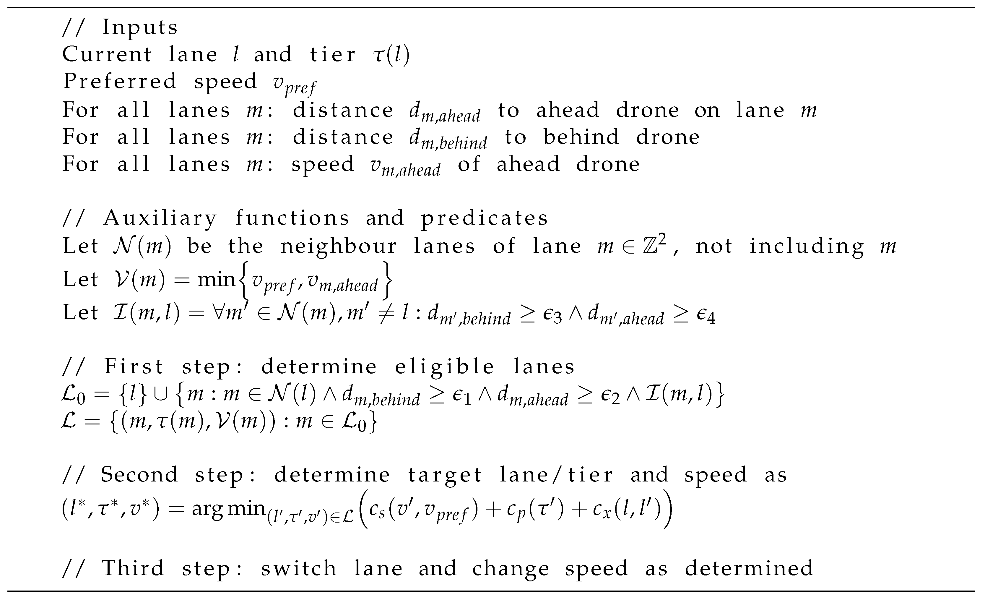
The GreedyLS algorithm proceeds in the following steps:

• First step: build the list $\mathcal{L}=\left\{(l_1^{\prime },{\tau }_1^{\prime },v_1^{\prime }),\dots ,(l_k^{\prime },{\tau }_k^{\prime },v_k^{\prime })\right\}$ of eligible lanes $l_i^{\prime }$ (and their tiers ${\tau }_i^{\prime }$) and allowable speeds $v_i^{\prime }$ on them:

  -

  The current lane l in tier $\tau$ is always eligible, its allowable speed is

  $$v^{\prime }=min\left\{v_{ahead},v_{pref}\right\}$$

  (3)

  where $v_{pref}$ is the own preferred speed.

  -

  A neighbour lane m is eligible when both the following conditions are true:

  *

  $d_{m,behind}\ge {ϵ}_1$, i.e., the distance to the behind drone must be at least as large as a given threshold ${ϵ}_1$.

  *

  $d_{m,ahead}\ge {ϵ}_2$, i.e., the distance to the ahead drone must be at least as large as a given threshold ${ϵ}_2$.

  These conditions together express that we only consider a neighbour lane eligible when there is a sufficiently large “gap” around our current position.

  -

  The previous eligibility conditions can be extended to better address a particular type of collision, which we loosely refer to as “concurrent collisions”. These can occur if two (or more) drones on different lanes find the same target lane m eligible and decide to switch to it at the same time and position. To prevent this, the previous eligibility conditions for neighbour lane m can be extended to require that all neighbour lanes $m^{\prime }$ of m excluding our own current lane l (we refer to these as indirect neighbours of lane l) have a sufficiently large “gap”, i.e.,:

  *

  $\forall m^{\prime }\ne l,m^{\prime }\mathrm{is} \mathrm{neighbour} \mathrm{of} \mathrm{m}:d_{m^{\prime },behind}\ge {ϵ}_3$, i.e., the distance to the behind drone in lane $m^{\prime }$ must be at least as large as ${ϵ}_3$ for all neighbour lanes $m^{\prime }\ne l$ of target lane m.

  *

  $\forall m^{\prime }\ne l,m^{\prime }\mathrm{is} \mathrm{neighbour} \mathrm{of} \mathrm{m}:d_{m^{\prime },ahead}\ge {ϵ}_4$, i.e., the distance to the ahead drone in lane $m^{\prime }$ must be at least as large as ${ϵ}_4$ for all neighbour lanes $m^{\prime }\ne l$ of target lane m.

  -

  The allowable speed on the eligible neighbour lane m is given as

  $$v_m^{\prime }=min\left\{v_{pref},v_{m,ahead}\right\}$$

  (4)

• Second step: From $\mathcal{L}$ determine the target lane/tier and speed as

  $$(l^{*},{\tau }^{*},v^{*})=\underset{(l^{\prime },{\tau }^{\prime },v^{\prime })\in \mathcal{L}}{arg\; min}\left(c_s(v^{\prime },v_{pref})+c_p\left({\tau }^{\prime }\right)+c_x(l,l^{\prime })\right)$$

  (5)

  i.e., the lane/tier and speed combination giving the smallest total position, speed and switching cost per unit of time. The term $c_x(l,l^{\prime })$ allows to model a cost for switching into a neighboured lane, it is of the form $c_x(l,l^{\prime })={ϵ}_5·{\mathbf{1}}_{\left\{l^{\prime }\right\}}\left(l\right)$, where ${\mathbf{1}}_{\left\{l^{\prime }\right\}}\left(l\right)=1$ if $l=l^{\prime }$ and 0 otherwise. The parameter ${ϵ}_5\ge 0$ represents lane switching cost.
• Third step: Switch to lane $l^{*}$ and adjust speed to $v^{*}$.

A pseudo-code summary of this algorithm can be found in Figure 3.

For the purposes of this paper, we assume that

$$c_p\left(\tau \right)=\left\{\begin{array}{ccc}\hfill 0& :& \hfill \tau \le 1\\ \hfill {\kappa }_1{(\tau -1)}^2& :& \hfill \tau >1\end{array}\right.$$

(6)

for some ${\kappa }_1\ge 0$, i.e., we assume that the intra-tube part consists of the centre lane and only one tier around it. We furthermore assume that

$$c_s(v,v_{pref})={\kappa }_2{(v-v_{pref})}^2$$

(7)

for some ${\kappa }_2\ge 0$. Both speeds v and $v_{pref}$ are assumed to be given in units of m/s. Note that the two functions $c_p(·)$ and $c_s(·)$ are not considered part of the GreedyLS algorithm proper, but are just examples chosen for the purposes of this paper. By changing the cost function $c_p(·)$ we can model other tube layouts, e.g., we can include more tiers, or we can rule out lanes that would collide with buildings by assigning them infinite costs. The remaining GreedyLS algorithm can remain unchanged.

Note that the behaviour of this algorithm is determined by the five constants ${ϵ}_1$ to ${ϵ}_5$ as well as the position and speed cost per unit time mappings $c_p(·)$ and $c_s(·)$ (in our case, in particular the constants ${\kappa }_1$ and ${\kappa }_2$). In addition to and independently of this algorithm, each drone should nearly continuously monitor the distance to the ahead drone on the same lane. This distance can change instantaneously, for example, when another drone switches into our lane ahead of us. In response to such a change, we need to adapt our own speed immediately to the speed of the new ahead drone (by adjusting our own speed to the minimum of the ahead drone speed and our own preferred speed).

4.2. Baseline Algorithm and GreedyLS Variants

To limit the scope of the evaluation in this paper we make some preliminary choices for some of the GreedyLS parameters, and then define a baseline algorithm and a number of GreedyLS variants to compare.

With one exception, we will set ${ϵ}_5=0$, i.e., in this paper we ignore lane-switching costs. We set ${ϵ}_1={ϵ}_2={ϵ}_1^{*}$, i.e., we assume that in neighboured lanes the required gap has the same size ahead and behind. In our experiments, we only vary ${ϵ}_1^{*}$. We also set ${ϵ}_3={ϵ}_4={ϵ}_2^{*}$, i.e., we assume that the required gap in the neighbour lanes (to avoid concurrent collisions) has the same size ahead and behind. In our experiments, we vary only ${ϵ}_2^{*}$. In particular, we choose either ${ϵ}_2^{*}=0$, effectively disabling the check for concurrent collisions, or we set ${ϵ}_2^{*}$ to be the same as ${ϵ}_1^{*}$, and only the latter is varied.

The baseline algorithm considered in this paper is referred to as the Blind algorithm. In this, an inserted drone never changes its lane or speed at all, i.e., it reflects the situation where drones do nothing at all to avoid collisions. In addition, we define the following four GreedyLS variants:

• Defensive algorithm: pick ${\kappa }_1={\kappa }_2=1$, ${ϵ}_1^{*}={ϵ}_2^{*}={10}^9$ and ${ϵ}_5={10}^9$. These settings effectively rule out any lane switching but allow for adaptation to the speed of the ahead node on the current lane.
• Crowded-$({ϵ}_1^{*},{ϵ}_2^{*})$ algorithm: restrict to intra-tube lanes by setting ${\kappa }_1={10}^9$ (cf. Equation (6)), ${\kappa }_2=1$ and ${ϵ}_1^{*}$, ${ϵ}_2^{*}$ to the given values.
• PreferInside-$({ϵ}_1^{*},{ϵ}_2^{*})$: set ${\kappa }_1=25$ and ${\kappa }_2=1$. With these settings, an out-of-tube lane becomes preferable only when the best achievable speed difference to the preferred speed $v_{pref}$ on any eligible intra-tube lane exceeds 5 m/s.
• PreferOutside-$({ϵ}_1^{*},{ϵ}_2^{*})$: set ${\kappa }_1={\kappa }_2=1$. With these settings already modest speed differences to the preferred speed will make out-of-tube lanes more preferable.

For the last three algorithms, we have simulated the following combinations for $({ϵ}_1^{*},{ϵ}_2^{*})$:

• $(10,0)$, $(20,0)$, $(50,0)$;
• $(10,10)$, $(20,20)$, $(50,50)$.

We have summarized all relevant GreedyLS parameters (general decision algorithm parameters, parameters for example cost functions, and restrictions of general parameters used in this paper) in

Table 2. Key adjustable parameters of GreedyLS.

Parameter	Explanation	Value
Basic GreedyLS Decision Parameters
${ϵ}_1$	Required minimum distance to behind drone on a neighbour lane	varied
${ϵ}_2$	Required minimum distance to ahead drone on a neighbour lane	varied
${ϵ}_3$	Required minimum distance to behind drone on an indirect neighbour lane	varied
${ϵ}_4$	Required minimum distance to ahead drone on an indirect neighbour lane	varied
${ϵ}_5$	Lane-switching cost	0
Timing parameters
	Unit time	3 s
	Neighbour table timeout	10 s
Example cost function parameters
${\kappa }_1$	Position cost coefficient	varied
${\kappa }_2$	Speed cost coefficient	varied
GreedyLS parameter choices for this paper
${ϵ}_1^{*}$	Common value of ${ϵ}_1$ and ${ϵ}_2$ (required minimum distance to ahead and behind drones on neighbour lanes)	varied
${ϵ}_2^{*}$	Common value of ${ϵ}_3$ and ${ϵ}_4$ (required minimum distance to ahead and behind drones on indirect neighbour lanes)	varied

.

4.3. Further Comments

Algorithm Scope: It is important to point out that the GreedyLS algorithm is not limited to the case with just two in-tube tiers of lanes, but rather can accommodate arbitrary layouts of in-tube, allowed out-of-tube and completely forbidden lanes (e.g., ones that would go through a building). This can be achieved through proper choice of the position cost function $c_p(·)$, which in general can be made location- or time-dependent, and which may even be adapted over time. A reliable system then needs to be in place to ensure that drones always have access to the most recent position cost function relevant for their movements.

Algorithm Complexity: Fix a particular drone x and denote by M the number of current neighbour drones of x. For each of these neighbour drones we know its position, its lane, and its speed from the beacons we have received from it and which have been entered into the neighbour table. There are three key operations for the neighbour table: enumerating all neighbours and finding those on a particular lane, adding a new neighbour and periodically checking the timers associated with each neighbour (and possibly deleting a timed-out neighbour from the table). Each of these operations is $O\left(M\right)$ at worst. If we denote by $L=1+6+12=19$ the number of lanes that the algorithm considers (the current lane, the six neighbour lanes and the 12 indirect neighbour lanes), then for each of these L lanes the GreedyLS algorithm needs to find out which drones are on that lane and in particular the position and speed of the ahead and behind drones, which for each of the L lanes is an $O\left(M\right)$ operation at worst (and better with suitable data structures). The first step of the decision algorithm is $O\left(1\right)$, since for each of the six neighbour lanes we test the distance to the ahead and behind drones on that lane and its six neighbours (indirect neighbour check). The first step produces a result list with up to six candidate lanes, and in the second step we evaluate the cost function (Equation (5)) for each of the candidate lanes, which is an $O\left(1\right)$ operation per candidate lane.

Handling Uncertainty: In a drone road system there will be various and substantial uncertainties and disturbances, for example, wind gusts or noise in GPS position readings. Addressing these uncertainties explicitly will be the subject of future research, in this paper, we focus solely on the uncertainty induced by the underlying communications system (and the packet losses it induces). We clearly expect that new decision algorithms will be developed that account for such uncertainty, but they will also be addressed in many other ways, e.g., through advances in GPS receiver technology, through appropriate system settings (for example, making lanes wider), and through specifying minimum technical quality requirements for participating drones.

5. Results

We have built a discrete-event simulation model using the OMNeT++ simulation framework (https://www.omnetpp.org (accessed on 13 October 2022)) and using the IEEE 802.11 EDCA implementation provided by the INET framework in version 4.3.2. (https://inet.omnetpp.org (accessed on 13 October 2022)).

In our simulations, we ran 50 independent replications for each considered parameter combination, and we present averaged results. We have also checked the 95% confidence intervals of our calculated averages. These are sufficiently tight, and we have not included them in the figures to avoid visual clutter. Each replication ran for 200 simulated seconds.

5.1. Average Number of Collisions

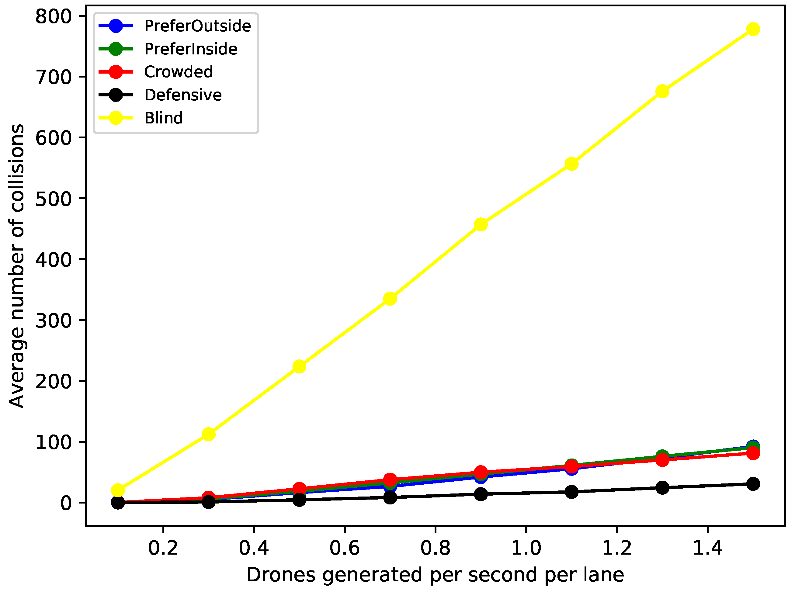
In Figure 4, we show results for the average number of collisions per kilometre for varying drone generation rate $\lambda$, a tube length of $L=1$ km and all considered variants, including the Blind variant. The curve shown for each variant is its average performance over all combinations of beaconing rate $\beta$ and $({ϵ}_1^{*},{ϵ}_2^{*})$ combinations. Obviously, the Blind variant is substantially worse than all the other variants, so we will not discuss it any further. In Figure 5, we show results for the average number of collisions for all schemes except the blind one, and for three different beaconing rates $\beta \in \left\{5\mathrm{Hz},10\mathrm{Hz},20\mathrm{Hz}\right\}$. For each of the Crowded, PreferInside and PreferOutside algorithms we have selected a $({ϵ}_1^{*},{ϵ}_2^{*})$ combination with (close to) the lowest number of collisions for inclusion in the graph.

The first (and quite obvious) conclusion is that all considered algorithms provide vast improvements over the Blind algorithm, which we only included as a baseline in the first place. Its performance in the other metrics is clear from its construction: surviving drones will always fly at their preferred speed (hence producing an average speed of 25 m/s) and they will never leave the tube.

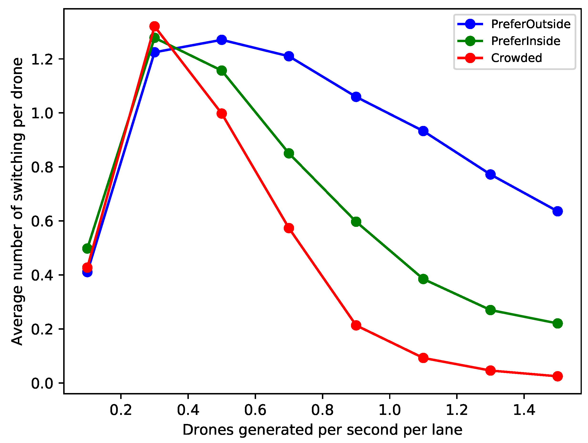
The Defensive algorithm shows consistently the best performance, having a genuinely lower average collision rate than any other algorithm. Note that the Defensive algorithm effectively forbids any lane switching, whereas all the other algorithms allow it (either restricted to in-tube lanes or not). This suggests that allowing lane switching increases collision risk. To investigate this further, in Figure 6 we show the average number of lane-switching operations per drone for selected algorithms. The figure confirms that the algorithm allowing the most lane switching operations (PreferOutside) is also the algorithm showing the highest average number of collisions for higher values of the drone generation rate. The Crowded algorithm shows a “non-monotonic” behaviour in Figure 5, its collision rate actually decreases at some point for increasing $\lambda$. This can also be explained with reference to Figure 6. The Crowded algorithm is effectively limited to in-tube lanes, and these leave fewer and fewer options for lane switching, so that as $\lambda$ increases the Crowded algorithm behaves more and more like the Defensive algorithm, leading to a reduction in collisions.

It is also noteworthy to point out the differences between the beaconing rates in Figure 6. The relative performance of the considered algorithms changes, but clearly the overall average collision numbers increase for decreasing beaconing rate.

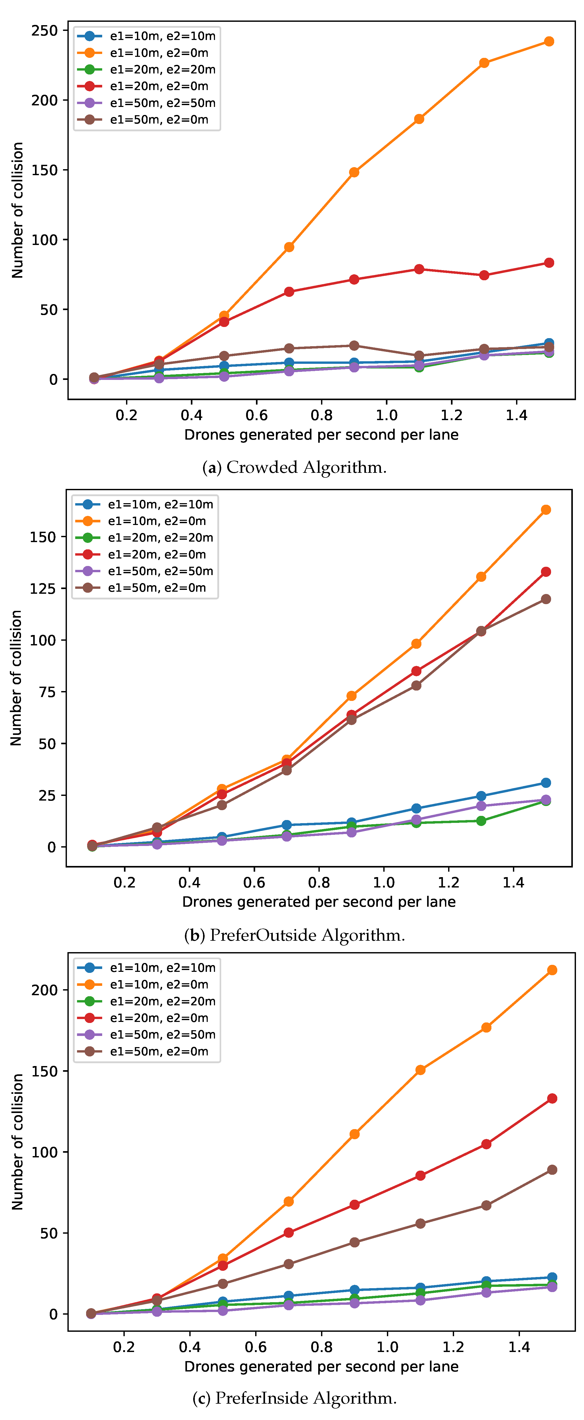
To investigate the role that concurrent collisions play (see Section 4.1), in Figure 7 we show the average collision count for the considered combinations of $({ϵ}_1^{*},{ϵ}_2^{*})$ and an average beaconing rate of $\beta =20$ Hz for the for Crowded, PreferOutside and PreferInside algorithms (cf., Section 4.2). It can be observed that for all three algorithms, the variants which disable the check for concurrent collisions show much higher collision counts than the variants which do check for the risk of concurrent collisions and the difference can be quite substantial. Note that for each of these three algorithms we have included the overall (close-to) top-performing variant (with $({ϵ}_1^{*},{ϵ}_2^{*})=(10\mathrm{m},10\mathrm{m})$) in Figure 5 and in all subsequent figures.

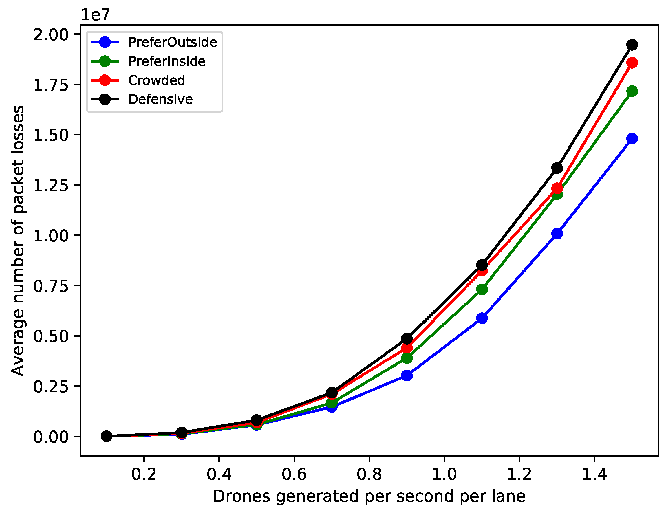
The number of drone collisions increases for all algorithms as the drone generation rate $\lambda$ increases. Clearly, the higher drone density packs drones more closely and also leads to more packet collisions (either direct or hidden-terminal collisions), which in turn leads to higher uncertainty about the position and speed of neighboured drones, including the ones that are close and pose the highest collision risk. To shed further light on this, in Figure 8 we show the average number of packet losses (as a proxy for packet collision rates), which we have inferred from sequence number gaps observed by receiving nodes. In this figure, we have used a beaconing rate of 20 Hz. As expected, the number of packet losses increases quickly for increasing drone density. The observation that the Defensive, Crowded and PreferInside variants show a higher packet loss count than PreferOutside is likely due to the fact that these variants produce fewer drone collisions than PreferOutside, leading to a higher drone density and, therefore, more packet losses.

It can also be observed that in general the curves for the higher beaconing rate $\beta =20\mathrm{Hz}$ show better performance over the lower rate $\beta =10\mathrm{Hz}$. Likely, the higher beacon generation rate, while increasing channel congestion, still reduces the average time between receiving beacons from a neighbour, therefore, reducing uncertainty about its position and collision risk. It can be expected though that further increases the beaconing rate are going to increase the collision risk, due to increasing hidden-terminal packet collisions [12].

5.2. Average Speed

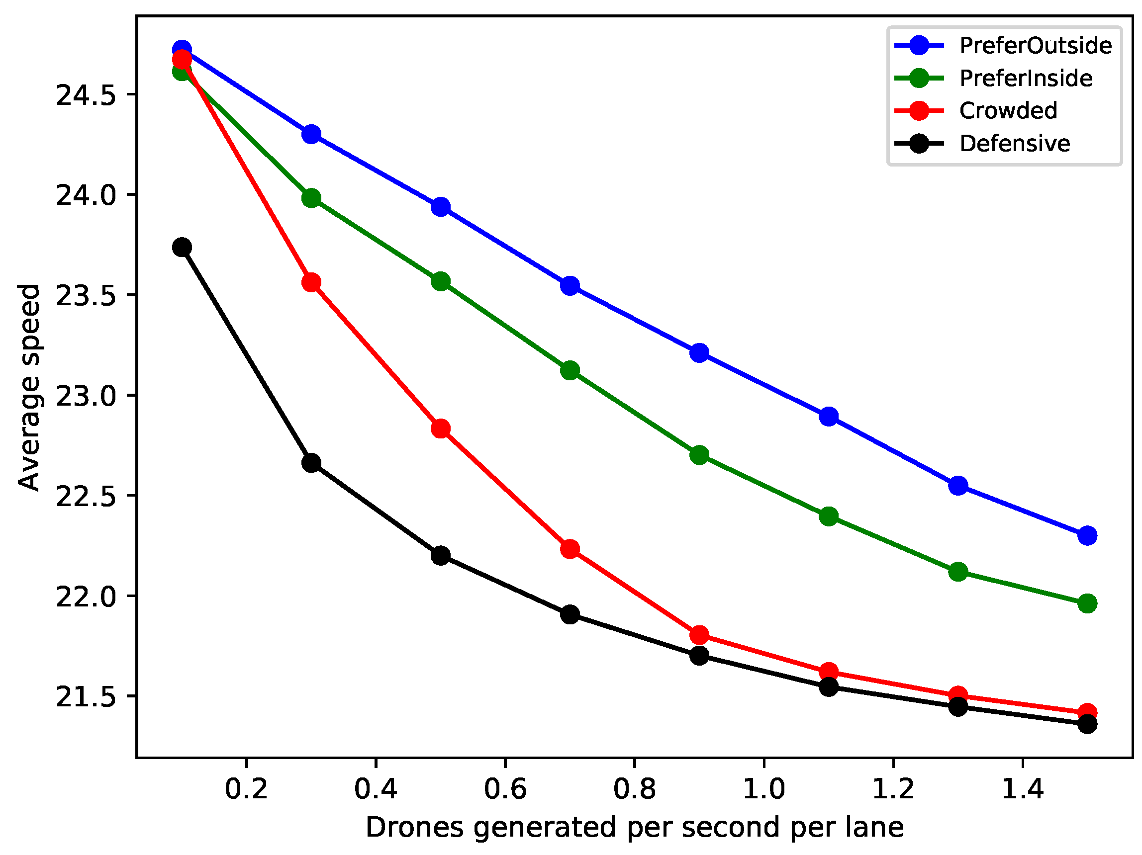
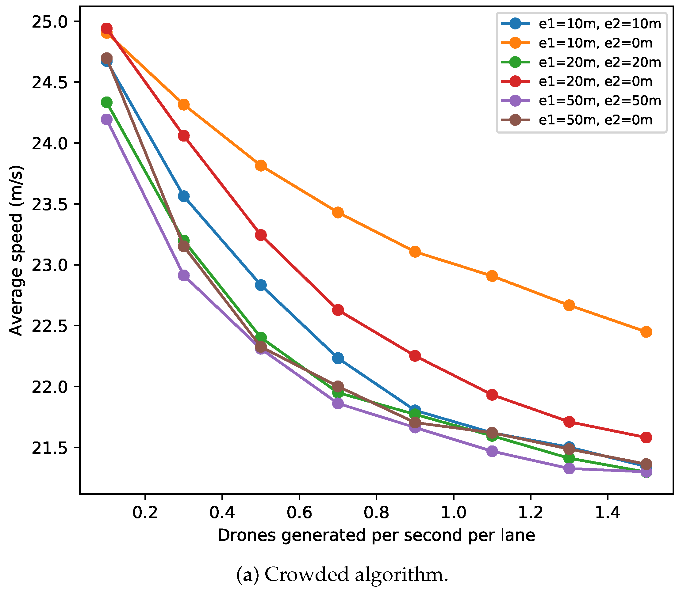
In Figure 9 we show the average speed of drones for varying drone generation rate $\lambda$, for the Defensive algorithm and the best variants of the Crowded/PreferOutside/PreferInside algorithms as identified in the previous section. As the preferred speeds are drawn from the interval $[20\mathrm{m}/\mathrm{s},30\mathrm{m}/\mathrm{s}]$, we would expect this average to be 25 m/s if drones avoid slowing down.

As expected, for all algorithms the average speed decreases as the drone generation rate increases, as there is a higher chance that a drone might have to slow down to adapt to the speed of an ahead drone, while simultaneously having fewer options for lane switching. The Defensive algorithm shows this effect most strongly, as lane switching is effectively ruled out. The Crowded algorithm has second-worst performance, followed by PreferInside, as both algorithms have a tendency to restrict drones to intra-tube lanes. With the PreferOutside algorithm, drones have a stronger tendency to move into out-of-tube lanes, leading to an overall larger number of lanes being used and a lower drone density per lane, which in turn allows for higher speeds. However, recall from Section 5.1 that the PreferOutside algorithm also tends to have the highest collision count for large $\lambda$.

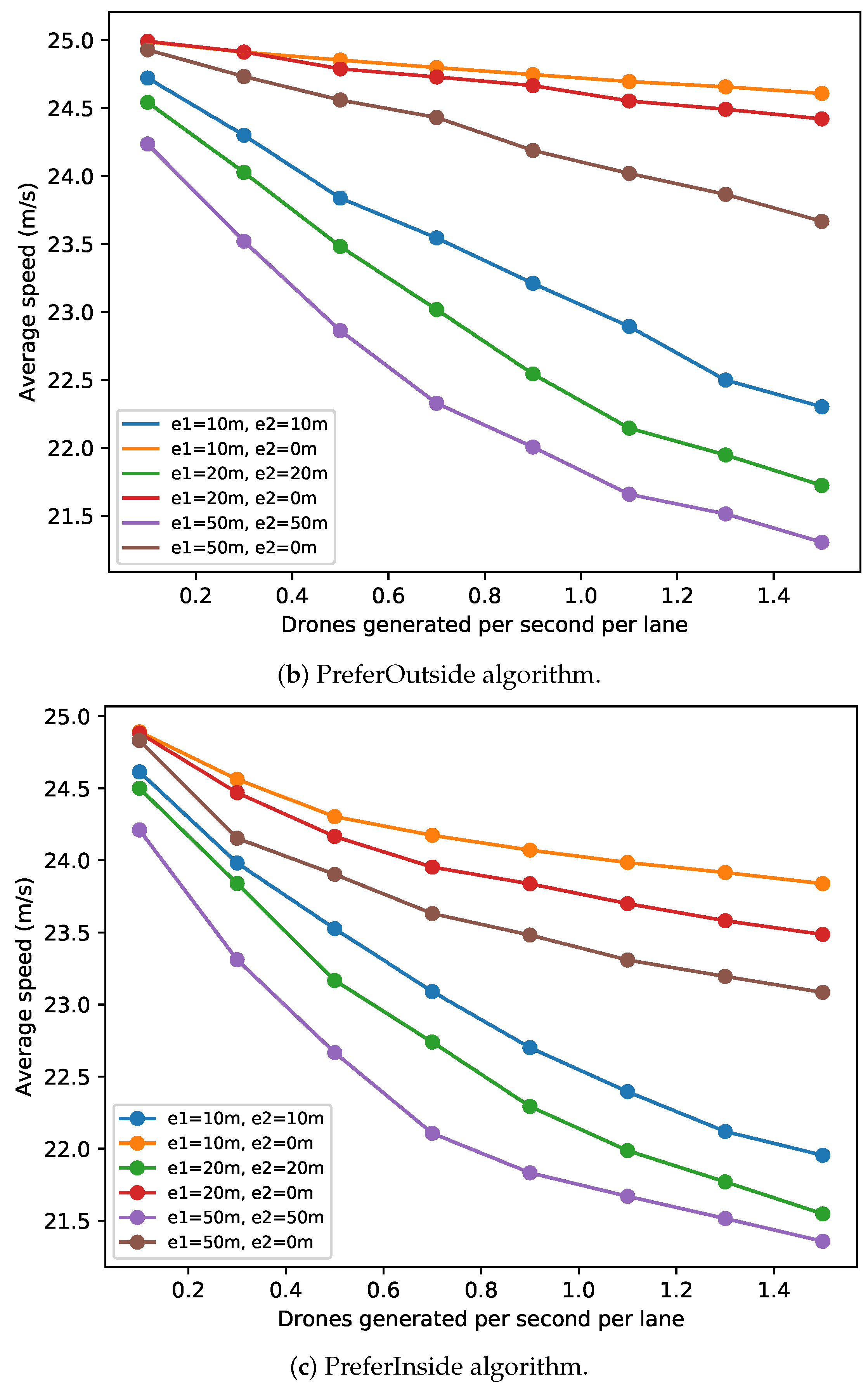
We have also investigated the average speed for the different choices of $({ϵ}_1^{*},{ϵ}_2^{*})$ for the Crowded, PreferOutside and PreferInside algorithms (cf., Section 4.2). The results are shown in Figure 10. It can be observed that for all three algorithms the variant that was the best in terms of collision count also had the lowest average speeds, particularly as $\lambda$ increases.

5.3. Average Out-of-Tube Tier

In Figure 11, we show the average out-of-tube tier of drones for the varying drone generation rate $\lambda$. Note that algorithms forcing drones to stay inside the tube (Defensive and Crowded) incur a cost of zero, as confirmed in the figure. For the PreferOutside and PreferInside algorithms, the figure confirms that it is indeed possible to achieve different positional behaviours through careful selection of algorithm parameters.

We have investigated the average out-of-tube tier values for the different choices of $({ϵ}_1^{*},{ϵ}_2^{*})$ for the PreferOutside and PreferInside algorithms. For both algorithms, the variant with the lowest average collision count also had the lowest average out-of-tube tier values as $\lambda$ increases. This is because the variant that includes the most conservative concurrent collision checks is also the most reluctant to switch lanes overall, which also reduces lane-switching operations to out-of-tube lanes.

5.4. Discussion

Our results already allow drawing some conclusions. The observation that collision rates increase as the drone density increases is quite expected, and this can certainly in parts be attributed to increased packet loss rates and the resulting increased uncertainty about the positions and speed of neighboured drones.

The presence or absence of a check for concurrent collisions can have a substantial impact on collision rates, and on the willingness of drones to switch lanes. Related to this is the observation that lane switching generally increases the collision risk, even when drones might move out of the tube. At the same time, avoiding lane switching comes at the cost of average speed. Interestingly, the completely rigid Defensive algorithm has a much lower collision count than the much more flexible PreferOutside algorithm, which ought to have plenty of opportunities for drones to avoid collisions by leaving the tube and reducing drone density.

Our results also show a tradeoff between collision count and speed or drone density and one can expect that these tradeoffs will be experienced by any decision algorithm.

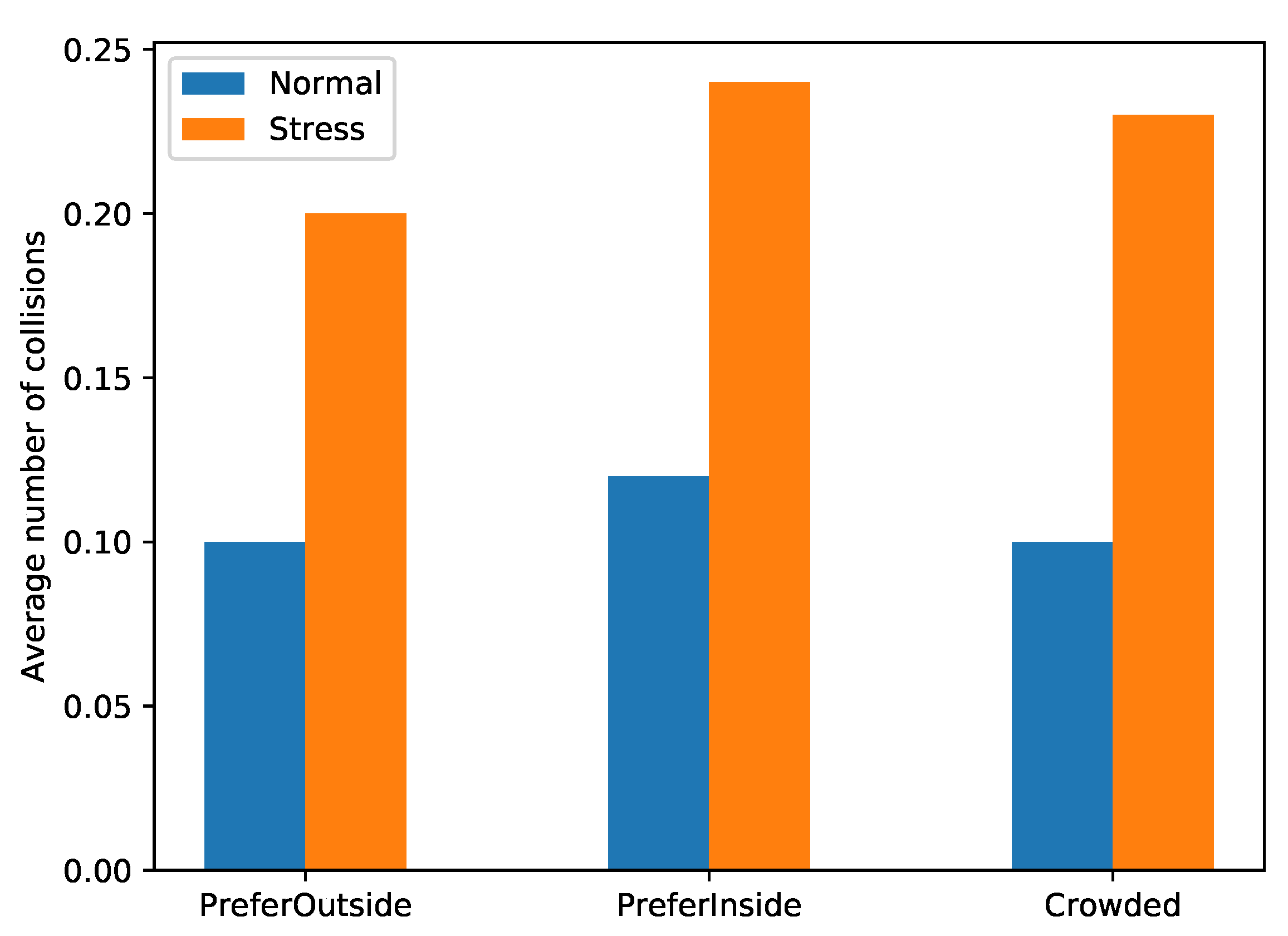
Finally, as explained in Section 3.6, for the simulation results presented so far we have chosen parameters that “stress” the system, leading to a perhaps heightened number of collisions. To give a glimpse at the impact of this choice, as an example we show in Figure 12 the average number of collisions for the PreferOutside, PreferInside and Crowded algorithms, in both a “stressed” setting (using the same parameters as previously) and a “normal” setting with more relaxed parameters. In the normal setting, we have used a generation rate of 0.1 drones generated per second per lane, ${ϵ}_1^{*}={ϵ}_2^{*}=10\mathrm{m}$, a distance of 10 m between lane centre points, a uniform distribution between 10 m/s and 15 m/s for the preferred speed, a 20 Hz beaconing rate and a 10 minimum safety distance $d_{safety}$ between inserted drones. It can be seen that indeed the average collision numbers are substantially lower for the normal setting, while relative performance trends between schemes are broadly preserved.

6. Conclusions and Future Work

The construction of a drone road system offers a principled way forward to use drones on a larger scale for deliveries of small goods and other applications in urban environments. Controlling the movements of drones in such a system should follow a distributed approach for scalability reasons. We believe that any decision algorithm by which a drone decides its lane and speed will face the tradeoffs that we have observed, for example, the tradeoff between collision risk and speed or drone density.

Besides its ability to let users adjust their operating points in these tradeoffs by careful parameter selection, the simple decision algorithm presented in this paper is mainly useful as a baseline for more advanced algorithms incorporating additional sensor modalities or additional information exchanged between drones (including active negotiation).

There are many opportunities for future research. The first is to extend the system model for a drone road system by intersections, on- and offramps, arbitrarily curved and oriented tubes and location-dependent cost functions for the speed and position cost, $c_p(·)$ and $c_s(·)$, to accommodate differences in built infrastructure in various parts of a city. Building on such an extended system model, there are then opportunities to design suitable decision algorithms for turning at an intersection or zipping in at onramps. An important addition to the system model (and perhaps to future decision algorithms) will be the explicit consideration of system uncertainty, e.g., positional uncertainty from noisy GPS readings or wind gusts. The system model can also be extended to include a more realistic model of drone dynamics and decision algorithms then can express more fine-grained behaviour for acceleration and deceleration, perhaps including more aspects of the behaviour of human drivers. Beyond this, we can optimize important system parameters such as the beaconing rate, physical layer parameters such as transmit power or the modulation and coding scheme and the parameters of the GreedyLS algorithm, and perform a sensitivity study for these parameters. Besides offline optimization, it is also very interesting to find dynamic adaptation algorithms for particularly important parameters such as the beaconing rate. Finally, since serious experimental work in the construction of drone road systems is still far ahead in the future, it will be quite important to develop simulation tools allowing the efficient simulation of large-scale road systems while preserving important properties of the wireless communications technology and sensors.