Decentralized Sampled-Data Fuzzy Tracking Control for a Quadrotor UAV with Communication Delay

Abstract

This study deals with the decentralized sampled-data fuzzy tracking control of a quadrotor unmanned aerial vehicle (UAV) considering the communication delay of the feedback signal. A decentralized Takagi–Sugeno (T–S) fuzzy approach is adopted to represent the quadrotor UAV as two subsystems: the position control system and the attitude control system. Unlike most previous studies, a novel decentralized controller considering the communication delay for the position control system is proposed. In addition, to minimize the increase in computational complexity, the Lyapunov–Krasovskii functional (LKF) is configured as the only state required for each subsystem. The design conditions guaranteeing the tracking performance of the quadrotor UAV are derived as linear matrix inequalities (LMIs) that are numerically solved. Lastly, the validity of the proposed design method is verified by comparing the results through simulation examples with and without communication delay.

1. Introduction

In recent decades, quadrotor unmanned aerial vehicles (UAVs) have been utilized in many fields, including civil and military, due to their excellent hovering, simple mechanical structure, and low maintenance cost. However, it is not easy to analyze and design a control system because the dynamics of a quadrotor UAV is nonlinear. In addition, the quadrotor UAV is an underactuated system with 6 degrees of freedom using 4 thrusts generated from 2 pairs of rotors rotating in opposite directions. To resolve these difficulties, studies were conducted on applying various control techniques to control quadrotor UAVs [1], such as PID control [2,3,4,5] and LQR control [6,7,8,9,10] as a linear control method and backstepping control [11,12,13,14], sliding mode control [13,14,15,16,17,18,19], and fuzzy control [20,21,22,23,24,25,26,27] as a nonlinear control method. As for the linear control technology, although PID control is easy to implement and LQR control can cope with disturbances, the dynamics of quadrotor UAV has nonlinearity and have to be linearized, so their performance is somewhat limited. As nonlinear control techniques, backstepping control and sliding-mode control are widely used to design a robust control system that can cope with disturbances, but the former is difficult to implement, and the latter has difficultly in coping with the chattering effect.

Recently, the Takagi–Sugeno (T–S) fuzzy approach has received considerable attention [28,29]. The T–S fuzzy approach is a nonlinear control technique that represents a given nonlinear system as the convex sum of its linear subsystems, so existing linear control techniques are easily applicable [30]. Therefore, there are many studies to control quadrotor UAVs through T–S fuzzy modeling. In early studies related to this, the dynamics of a complex quadrotor UAV was presented as a single T–S fuzzy model to design a controller [20,21]. Meanwhile, focusing on the fact that the quadrotor UAV is an underactuated system, and the computational complexity increases due to the large dimension of dynamics, a study applied a decentralized control technique that divided the entire system into subsystems to control them [23]. However, since the above-mentioned studies were carried out on the continuous time domain, it is difficult to apply it to a quadrotor UAV implemented by digital hardware. From this perspective, the authors of [27] recently represented a quadrotor UAV as a decentralized T–S fuzzy model and proposed a decentralized sampled-data fuzzy controller design method. In short, decentralized control and sampled-data control are required to design a control system for a quadrotor UAV, so more studies applying them need to be conducted.

On the other hand, memory sampled-data control considering both the sampling and time delay of a feedback signal was actively studied in recent years [31,32,33,34,35]. In particular, such a control technique was applied to a multiagent system having a structure in which a control system received a state with a time delay of another system through communication [36,37,38]. The quadrotor UAV receiving the feedback signal from the outside also sufferred from the communication delay. In this regard, on the basis of memory sampled-data control, the tracking performance could be improved because the delayed signal could be effectively handled. Therefore, it is necessary to study the control system for a quadrotor UAV considering the communication delay of the feedback signal.

From this point of view, we propose a sampled-data fuzzy control technique for quadrotor UAVs considering the communication delay of the feedback signal. Since the feedback signal received from the outside of the quadrotor UAV is the state of the position, it is necessary to control the quadrotor UAV system by dividing it into a position control system and an attitude control system. Therefore, in this study, the quadrotor UAV is expressed as the position control system and the attitude control system through decentralized T–S fuzzy modeling, and a decentralized controller design technique is provided. A novel controller is proposed to consider the delayed state only in the position control system, and a novel Lyapunov–Krasovskii functional (LKF) for this is also introduced. The conditions for ensuring the stability of tracking error dynamics of quadrotor UAV and tracking performance are formulated as an optimal problem in the form of linear matrix inequalities (LMIs). Lastly, simulation examples are provided to prove the feasibility of the proposed design technique. The main contributions of this study are summarized as follows:

• A novel sampled-data fuzzy tracking controller structure that consists of two different types of decentralized controllers for a quadrotor UAV with communication delay is proposed.
• The LKF introduced in most previous studies on memory sampled-data control is improved to minimize computational complexity due to dimensional increase from unnecessary states.

Notations: Throughout this paper, ${\mathbb{Z}}_{\ge 0}$ represents a set of all integers greater than or equal to zero. ${\mathcal{I}}_n$ denotes the integer set $\{1,2,\dots ,n\}$ for the positive integer n. $N\succ 0$ (resp. $N\prec 0$) implies that matrix N is positive (resp. negative) definite. ${\lambda }_N$ denotes the maximal eigenvalue of the $N^T\left(t\right)N\left(t\right)$. *, $\mathrm{Sym}\left\{N\right\}$, $\mathrm{col}\left\{\dots \right\}$, and $\mathrm{diag}\{\dots \}$ denote the symmetric elements of the symmetric matrix, $N+N^T$, the Euclidean norm for vectors, a column vector, and a block-diagonal matrix, respectively. $\mathbf{I}$ and $\mathbf{0}$ indicate the identity and the zero matrices of appropriate dimensions, respectively.

2. Preliminaries and Problem Formulation

In this section, we derive the T–S fuzzy model of tracking error dynamics of the quadrotor UAV. First, the dynamics of a quadrotor UAV are represented by two subsystems: a position control system and an attitude control system. Then, we derive the tracking error dynamics on the basis of T–S fuzzy modeling using the novel fuzzy controller proposed in this study. Lastly, a design problem is defined to clarify the conditions that should be satisfied to achieve the main purpose of this paper.

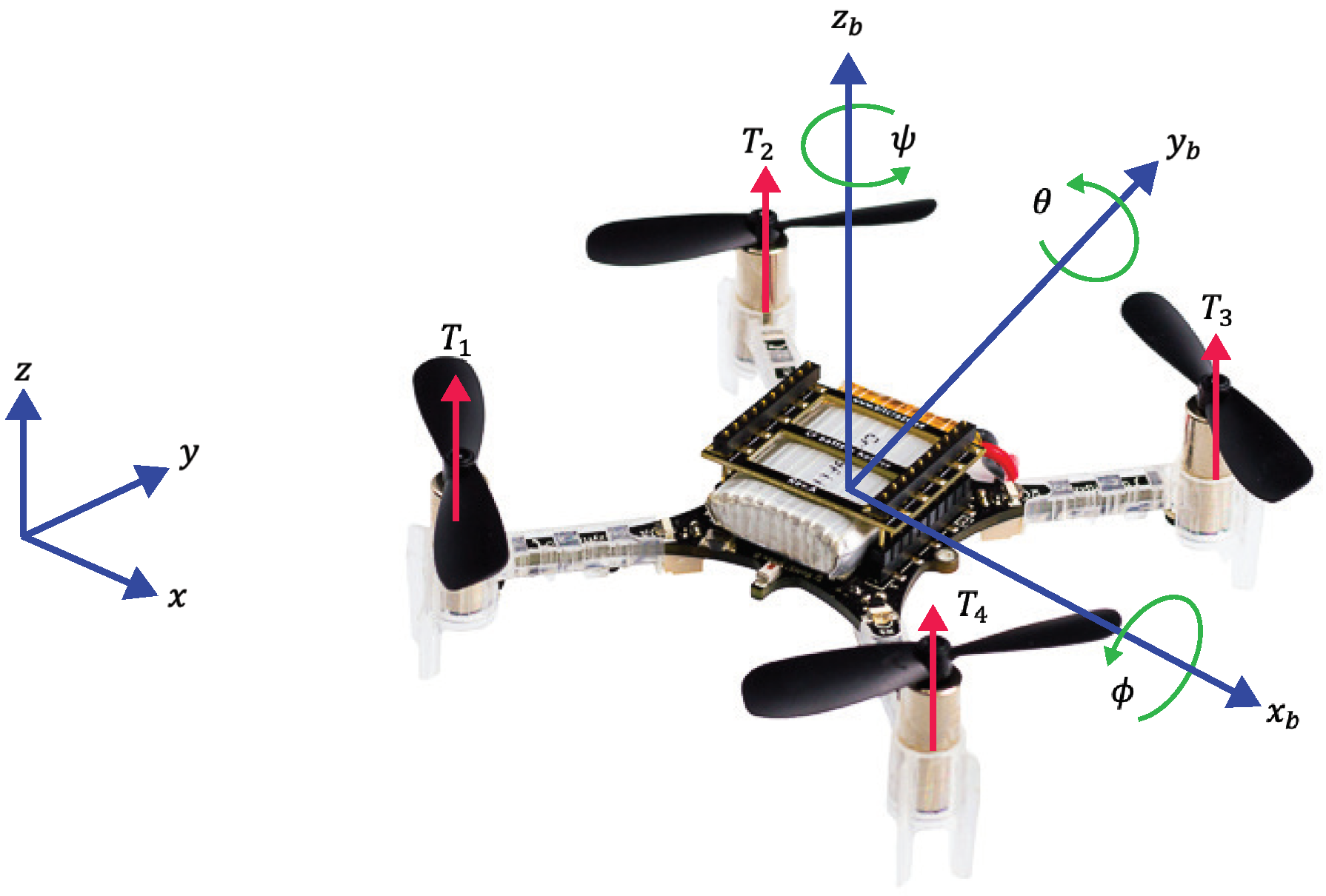
2.1. Dynamics of the Quadrotor UAV

In general, the dynamic behavior of a quadrotor UAV is described by $\left(x\right(t),y(t),z(t),$$\varphi \left(t\right),\theta \left(t\right),\psi \left(t\right))$, where $\left(x\left(t\right),y\left(t\right),z\left(t\right)\right)$ represent the position of the center of gravity of the quadrotor UAV in a given inertial frame, and $\left(\varphi \left(t\right),\theta \left(t\right),\psi \left(t\right)\right)$ are the Euler angles commonly called roll, pitch, and yaw, respectively [6]. Then, the dynamics of the quadrotor UAV considered in this paper is represented as follows [7,11]:

$$\begin{array}{c}\hfill \left\{\begin{array}{cc}\ddot{x}\left(t\right)\hfill & =(c_{{\varphi }_t}{s}_{{\theta }_t}{c}_{{\psi }_t}+s_{{\varphi }_t}{s}_{{\psi }_t})\frac{u_t\left(t\right)}{m}+{\Delta }_x\left(t\right)\hfill \\ \ddot{y}\left(t\right)\hfill & =(c_{{\varphi }_t}{s}_{{\theta }_t}{s}_{{\psi }_t}-s_{{\varphi }_t}{c}_{{\psi }_t})\frac{u_t\left(t\right)}{m}+{\Delta }_y\left(t\right)\hfill \\ \ddot{z}\left(t\right)\hfill & =c_{{\varphi }_t}{c}_{{\theta }_t}\frac{u_t\left(t\right)}{m}-g+{\Delta }_z\left(t\right)\hfill \\ \ddot{\varphi }\left(t\right)\hfill & =\frac{I_y-I_z}{I_x}\dot{\theta }\left(t\right)\dot{\psi }\left(t\right)+\frac{1}{I_x}{u}_{\varphi }\left(t\right)+{\Delta }_{\varphi }\left(t\right)\hfill \\ \ddot{\theta }\left(t\right)\hfill & =\frac{I_z-I_x}{I_y}\dot{\varphi }\left(t\right)\dot{\psi }\left(t\right)+\frac{1}{I_y}{u}_{\theta }\left(t\right)+{\Delta }_{\theta }\left(t\right)\hfill \\ \ddot{\psi }\left(t\right)\hfill & =\frac{I_x-I_y}{I_z}\dot{\varphi }\left(t\right)\dot{\theta }\left(t\right)+\frac{1}{I_z}{u}_{\psi }\left(t\right)+{\Delta }_{\psi }\left(t\right)\hfill \end{array}\right.\end{array}$$

(1)

where $s_{n_t}:=sin\left(n\left(t\right)\right)$ and $c_{n_t}:=cos\left(n\left(t\right)\right)$; $u_t\left(t\right)$, $u_{\varphi }\left(t\right)$, $u_{\theta }\left(t\right)$, and $u_{\psi }\left(t\right)$ denote the thrust, roll, pitch, and yaw inputs; m is the mass of the quadrotor UAV; g is the gravitational acceleration constant; $I_x$, $I_y$, and $I_z$ indicate the moment of inertia of each axis; ${\Delta }_x\left(t\right)$, ${\Delta }_y\left(t\right)$, ${\Delta }_z\left(t\right)$, ${\Delta }_{\varphi }\left(t\right)$, ${\Delta }_{\theta }\left(t\right)$, and ${\Delta }_{\psi }\left(t\right)$ represent the uncertain terms due to unmodeled dynamics.

The quadrotor dynamics (1) can be divided into the two following subsystems: the position control system $(l=1)$ and the attitude control system $(l=2)$ [27].

$$\begin{array}{cc}\hfill {\dot{\eta }}_l\left(t\right)& =A_l\left(t\right){\eta }_l\left(t\right)+B_l\left(t\right)u_l\left(t\right)+f_l\left(\eta \left(t\right)\right)\hfill \end{array}$$

(2)

where

$$\begin{array}{cc}\hfill \eta \left(t\right)& =\mathrm{col}\left\{{\eta }_1\left(t\right),{\eta }_2\left(t\right)\right\};\hfill \\ \hfill {\eta }_1\left(t\right)& =\mathrm{col}\left\{x\left(t\right),y\left(t\right),z\left(t\right),\dot{x}\left(t\right),\dot{y}\left(t\right),\dot{z}\left(t\right)\right\}=col\left\{{\eta }_{11}\left(t\right),\dots ,{\eta }_{16}\left(t\right)\right\};\hfill \\ \hfill {\eta }_2\left(t\right)& =col\left\{\varphi \left(t\right),\theta \left(t\right),\psi \left(t\right),\dot{\varphi }\left(t\right),\dot{\theta }\left(t\right),\dot{\psi }\left(t\right)\right\}=\mathrm{col}\left\{{\eta }_{21}\left(t\right),\dots ,{\eta }_{26}\left(t\right)\right\};\hfill \\ \hfill u_1\left(t\right)& =\mathrm{col}\left\{u_x\left(t\right),u_y\left(t\right),u_z\left(t\right)\right\},u_2\left(t\right)=\mathrm{col}\left\{u_{\varphi }\left(t\right),u_{\theta }\left(t\right),u_{\psi }\left(t\right)\right\};\hfill \\ \hfill f_1\left(\eta \left(t\right)\right)& =\mathrm{col}\left\{0,0,0,{\Delta }_x\left(t\right),{\Delta }_y\left(t\right),\left(\frac{c_{{\varphi }_t}{c}_{{\theta }_t}}{c_{{\varphi }_k}{c}_{{\theta }_k}}-1\right)g+{\Delta }_z\left(t\right)\right\};\hfill \\ \hfill f_2\left(\eta \left(t\right)\right)& =\mathrm{col}\left\{0,0,0,{\Delta }_{\varphi }\left(t\right),{\Delta }_{\theta }\left(t\right),{\Delta }_{\psi }\left(t\right)\right\};\hfill \\ \hfill A_1\left(t\right)& =\left[\begin{array}{cccccc}0& 0& 0& 1& 0& 0\\ 0& 0& 0& 0& 1& 0\\ 0& 0& 0& 0& 0& 1\\ 0& 0& 0& 0& 0& 0\\ 0& 0& 0& 0& 0& 0\\ 0& 0& 0& 0& 0& 0\end{array}\right];A_2\left(t\right)=\left[\begin{array}{cccccc}0& 0& 0& 1& 0& 0\\ 0& 0& 0& 0& 1& 0\\ 0& 0& 0& 0& 0& 1\\ 0& 0& 0& 0& a_1{\eta }_{26}\left(t\right)& 0\\ 0& 0& 0& a_2{\eta }_{26}\left(t\right)& 0& 0\\ 0& 0& 0& a_3{\eta }_{25}\left(t\right)& 0& 0\end{array}\right];\hfill \\ \hfill B_1\left(t\right)& =\left[\begin{array}{ccc}0& 0& 0\\ 0& 0& 0\\ 0& 0& 0\\ 1/m& 0& 0\\ 0& 1/m& 0\\ 0& 0& p_3\left(t\right)/m\end{array}\right];B_2\left(t\right)=\left[\begin{array}{ccc}0& 0& 0\\ 0& 0& 0\\ 0& 0& 0\\ b_1& 0& 0\\ 0& b_2& 0\\ 0& 0& b_3\end{array}\right]\hfill \end{array}$$

$u_x\left(t\right)=p_1\left(t\right)u_t\left(t\right)$; $u_y\left(t\right)=p_2\left(t\right)u_t\left(t\right)$; $u_z\left(t\right)=u_t\left(t\right)-\frac{mg}{c_{{\varphi }_k}{c}_{{\theta }_k}}$; $p_1\left(t\right)=c_{{\varphi }_t}{s}_{{\theta }_t}{c}_{{\psi }_t}+s_{{\theta }_t}{s}_{{\psi }_t}$; $p_2\left(t\right)=c_{{\varphi }_t}{s}_{{\theta }_t}{s}_{{\psi }_t}-s_{{\theta }_t}{c}_{{\psi }_t}$; $p_3\left(t\right)=c_{{\varphi }_t}{c}_{{\theta }_t}$; $a_1=\frac{I_y-I_z}{I_x}$; $a_2=\frac{I_z-I_x}{I_y}$; $a_3=\frac{I_x-I_y}{I_z}$; $b_1=\frac{1}{I_x}$; $b_2=\frac{1}{I_y}$; $b_3=\frac{1}{I_z}$.

2.2. T–S Fuzzy Model-Based Tracking Error Dynamics

The dynamics of the quadrotor UAV (2) shows that nonlinear terms exist in $A_2\left(t\right)$ and $B_1\left(t\right)$. In this subsection, we use the T–S fuzzy model-based control approach to deal with these nonlinear terms and derive tracking error dynamics of quadrotor UAV. The T–S fuzzy model for (2) is described by the following IF-THEN rule with $(l,i)\in {\mathcal{I}}_2\times {\mathcal{I}}_{r_l}$:

$$\begin{array}{cc}\hfill {\mathcal{R}}_l^i:& \mathrm{IF}{z}_{l1}\left(t\right)\mathrm{IS}{\Gamma }_{l1}^i\mathrm{AND}\cdots \mathrm{AND}{z}_{l{p}_l}\left(t\right)\mathrm{IS}{\Gamma }_{l{p}_l}^i\hfill \\ \hfill & \mathrm{THEN}{\dot{\eta }}_l\left(t\right)=A_{li}{\eta }_l\left(t\right)+B_{li}{u}_l\left(t\right)+f_l\left(\eta \left(t\right)\right),\hfill \end{array}$$

(3)

where ${\mathcal{R}}_l^i$ denotes the ith rule for the lth subsystem; $z_{lq}\left(t\right)$ is a premise variable and ${\Gamma }_{lq}^i\left(t\right)$ is a fuzzy set for $z_{lq}\left(t\right)$ with $q\in {\mathcal{I}}_{p_l}$: $(p_1,p_2)=(1,2)$; $r_l$ denotes the number of fuzzy rules of each subsystem: $(r_1,r_2)=(2,4)$; $A_{li}\in {\mathbb{R}}^{6\times 6}$ and $B_{li}\in {\mathbb{R}}^{6\times 3}$ are system matrices; $f_l\left(\eta \left(t\right)\right)\in {\mathbb{R}}^6$ is the unknown piecewise continuous vector function of $\eta \left(t\right)$ representing the interconnection terms and modeling uncertainty terms satisfying the following assumption:

Assumption 1

([39]). Time-varying vector function $f_l\left(\eta \left(t\right)\right)$ is unknown, but satisfies

$$\begin{array}{c}\hfill f_l^T\left(\eta \left(t\right)\right)f_l\left(\eta \left(t\right)\right)\le {\left({\rho }_l\right)}^2{\eta }^T\left(t\right)F_l^T{F}_l\eta \left(t\right),\end{array}$$

where ${\rho }_l>0$ is a bound scalar of the interconnection terms and $F_l$ is a constant matrix of appropriate dimension.

Applying the general defuzzification method to (3), the lth subsystem can be inferred as follows:

$$\begin{array}{c}\hfill {\dot{\eta }}_l\left(t\right)=\sum _{i=1}^{r_l}{w}_{li}\left(z_l\left(t\right)\right){\displaystyle \{}{A}_{li}{\eta }_l\left(t\right)+B_{li}{u}_l\left(t\right)+f_l\left(\eta \left(t\right)\right){\displaystyle \}},\end{array}$$

(4)

where

$$\begin{array}{cc}\hfill A_{1i}& =\left[\begin{array}{cccccc}0& 0& 0& 1& 0& 0\\ 0& 0& 0& 0& 1& 0\\ 0& 0& 0& 0& 0& 1\\ 0& 0& 0& 0& 0& 0\\ 0& 0& 0& 0& 0& 0\\ 0& 0& 0& 0& 0& 0\end{array}\right],B_{1i}=\left[\begin{array}{ccc}0& 0& 0\\ 0& 0& 0\\ 0& 0& 0\\ 1/m& 0& 0\\ 0& 1/m& 0\\ 0& 0& {\chi }_{1i}/m\end{array}\right],\mathrm{for}i\in {\mathcal{I}}_{r1};\hfill \\ \hfill A_{2i}& =\left[\begin{array}{cccccc}0& 0& 0& 1& 0& 0\\ 0& 0& 0& 0& 1& 0\\ 0& 0& 0& 0& 0& 1\\ 0& 0& 0& 0& a_1{\chi }_{3i}& 0\\ 0& 0& 0& a_2{\chi }_{3i}& 0& 0\\ 0& 0& 0& a_3{\chi }_{2i}& 0& 0\end{array}\right],B_{2i}=\left[\begin{array}{ccc}0& 0& 0\\ 0& 0& 0\\ 0& 0& 0\\ b_1& 0& 0\\ 0& b_2& 0\\ 0& 0& b_3\end{array}\right],\mathrm{for}i\in {\mathcal{I}}_{r2};\hfill \\ \hfill w_{li}\left(z_l\left(t\right)\right)& :=\frac{{\mu }_{li}\left(z_l\left(t\right)\right)}{{\sum }_{j=1}^{r_l}{\mu }_{lj}\left(z_l\left(t\right)\right)};{\mu }_{li}\left(z_l\left(t\right)\right):={\Pi }_{q=1}^{p_l}{\Gamma }_{lq}^i\left(z_{lq}\left(t\right)\right);\hfill \end{array}$$

${\Gamma }_{lq}^i\left(z_{lq}\left(t\right)\right):{\mathcal{W}}_{z_{lq}}\subset \mathbb{R}\to {\mathbb{R}}_{[0,1]}$ is the membership function of $z_{lq}\left(t\right)$ on the compact set ${\mathcal{W}}_{z_{lq}}$; thus, $w_{li}\left(z_l\left(t\right)\right)\in [0,1]$ and ${\sum }_{i=1}^{r_l}{w}_{li}\left(z_l\left(t\right)\right)=1$. In (4), we designate the premise variable of the position control system as $p_3\left(t\right)=z_{11}\left(t\right)\in [-{\mathcal{M}}_1,{\mathcal{M}}_1]$ and the premise variables of the attitude control system as ${\eta }_{25}\left(t\right)=z_{21}\left(t\right)\in [-{\mathcal{M}}_2,{\mathcal{M}}_2]$ and ${\eta }_{26}\left(t\right)=z_{22}\left(t\right)\in [-{\mathcal{M}}_3,{\mathcal{M}}_3]$, where ${\mathcal{M}}_k$ with $k\in {\mathcal{I}}_3$ is a known positive scalar. Then, on the basis of sector nonlinearity concept [30], we have:

$$\begin{array}{cc}\hfill & w_{11}\left(z_1\left(t\right)\right)=\frac{z_{11}\left(t\right)-{\chi }_{12}}{{\chi }_{11}-{\chi }_{12}},w_{12}\left(z_1\left(t\right)\right)=1-w_{11}\left(z_1\left(t\right)\right),\hfill \\ \hfill & w_{21}\left(z_2\left(t\right)\right)={\Gamma }_{21}^1\left(z_{21}\left(t\right)\right){\Gamma }_{22}^1\left(z_{22}\left(t\right)\right),w_{22}\left(z_2\left(t\right)\right)={\Gamma }_{21}^1\left(z_{21}\left(t\right)\right){\Gamma }_{22}^2\left(z_{22}\left(t\right)\right),\hfill \\ \hfill & w_{23}\left(z_2\left(t\right)\right)={\Gamma }_{21}^2\left(z_{21}\left(t\right)\right){\Gamma }_{22}^1\left(z_{22}\left(t\right)\right),w_{24}\left(z_2\left(t\right)\right)={\Gamma }_{21}^2\left(z_{21}\left(t\right)\right){\Gamma }_{22}^2\left(z_{22}\left(t\right)\right),\hfill \\ \hfill & {\Gamma }_{21}^1\left(z_{21}\left(t\right)\right)=\frac{z_{21}\left(t\right)-{\chi }_{23}}{{\chi }_{21}-{\chi }_{23}},{\Gamma }_{21}^2\left(z_{21}\left(t\right)\right)=1-{\Gamma }_{21}^1\left(z_{21}\left(t\right)\right),\hfill \\ \hfill & {\Gamma }_{22}^1\left(z_{22}\left(t\right)\right)=\frac{z_{22}\left(t\right)-{\chi }_{32}}{{\chi }_{31}-{\chi }_{32}},{\Gamma }_{22}^2\left(z_{22}\left(t\right)\right)=1-{\Gamma }_{22}^1\left(z_{22}\left(t\right)\right),\hfill \\ \hfill & ({\chi }_{11},{\chi }_{12})=({\mathcal{M}}_1,-{\mathcal{M}}_1),\hfill \\ \hfill & ({\chi }_{21},{\chi }_{22},{\chi }_{23},{\chi }_{24})=(-{\mathcal{M}}_2,-{\mathcal{M}}_2,{\mathcal{M}}_2,{\mathcal{M}}_2),\hfill \\ \hfill & ({\chi }_{31},{\chi }_{32},{\chi }_{33},{\chi }_{34})=(-{\mathcal{M}}_3,{\mathcal{M}}_3,-{\mathcal{M}}_3,{\mathcal{M}}_3).\hfill \end{array}$$

Remark 1.

In (4), external disturbance was not considered. Since this study focused on decentralized control considering the communication delay of a quadrotor UAV, the effect of disturbance was excluded. There are studies that attenuated the effects of disturbances on the system in previous quadrotor control studies, which can be easily solved by using the$H_{\infty }$control [40,41].

Before proceeding, the shorthand notations for any matrix ${\mathcal{V}}_{li}$ were adopted to improve readability as follows:

$$\begin{array}{cc}\hfill & {\mathcal{V}}_l\left(w_l\left(t\right)\right):=\sum _{i=1}^{r_l}{w}_{li}\left(z_l\left(t\right)\right){\mathcal{V}}_{li},{\mathcal{V}}_l\left(w_l\left(t_k\right)\right):=\sum _{i=1}^{r_l}{w}_{li}\left(z_l\left(t_k\right)\right){\mathcal{V}}_{li}.\hfill \end{array}$$

In this study, the following linear reference model was considered to ensure the tracking control performance of the quadrotor UAV:

$$\begin{array}{c}\hfill {\dot{\eta }}_l^r\left(t\right)=A_l^r{\eta }_l^r\left(t\right)+B_l^r{r}_l\left(t\right),\end{array}$$

(5)

where ${\eta }_l^r\left(t\right)\in {\mathbb{R}}^6$ and $r_l\left(t\right)\in {\mathbb{R}}^3$ stand for the state and the bounded input vectors of reference model for the lth subsystem; $A_l^r\in {\mathbb{R}}^{6\times 6}$ denotes the predefined asymptotically stable matrix; $B_l^r\in {\mathbb{R}}^{6\times 3}$ is a constant matrix.

Now, we propose a novel decentralized sampled-data fuzzy tracking controller that considers the time delay of the position control system as follows:

$$\begin{array}{c}\hfill u_l\left(t\right):=K_l\left(w_l\left(t_k\right)\right){\displaystyle \{}(2-l){\epsilon }_l(t_k-\tau )+(l-1){\epsilon }_l\left(t_k\right){\displaystyle \}},\mathrm{for}t\in [t_k,t_{k+1}),\end{array}$$

(6)

where ${\epsilon }_l\left(t\right):={\eta }_l\left(t\right)-{\eta }_l^r\left(t\right)$ denotes the tracking error vector of lth subsystem; $K_{li}\in {\mathbb{R}}^{3\times 6}$ is a control gain matrix to be determined; $t_k>0$ for $k\in {\mathbb{Z}}_{\ge 0}$ is a kth sampling time that satisfies $t_{k+1}-t_k:=h_k\le h$, in which h is the maximum allowable sampling period; $\tau >0$ represents communication delay.

Remark 2.

Unlike the controller of [27], communication delay τ is taken into account in the controller of the position control system in this study. In fact, since the state and reference of position${\epsilon }_1\left(t\right)$ and $r_1\left(t\right)$ are received through communication with the outside, it is necessary to consider the communication delay.

Remark 3.

There are many recent studies using a sampled-data controller including time-delay called memory sampled-data control [31,32,35]. However, as shown in (6), this study proposes a novel controller structure that consists of two types of decentralized controllers, and enables the use of proper controllers to each subsystem: a sampled-data controller with communication delay as the position control system$(l=1)$and a sampled-data controller without communication delay as the attitude control system$(l=2)$. Deriving the theorem using this complex type of controller is challenging, as it requires introducing a different LKF for each control system, and this complicates the formula.

Then, from (4) and (5) with (6), the tracking error dynamics of lth subsystem can be derived as follows:

$$\begin{array}{cc}\hfill {\dot{\epsilon }}_l\left(t\right)& ={\dot{\eta }}_l\left(t\right)-{\dot{\eta }}_l^r\left(t\right)\hfill \\ \hfill & =A_l\left(w_l\left(t\right)\right){\eta }_l\left(t\right)+B_l\left(w_l\left(t\right)\right)K_l\left(w_l\left(t_k\right)\right)\left\{(2-l){\epsilon }_l(t_k-\tau )+(l-1){\epsilon }_l\left(t_k\right)\right\}\hfill \\ \hfill & +f_l\left(\eta \left(t\right)\right)-A_l^r{\eta }_l^r\left(t\right)-B_l^r{r}_l\left(t\right)\hfill \\ \hfill & =A_l\left(w_l\left(t\right)\right){\epsilon }_l\left(t\right)+B_l\left(w_l\left(t\right)\right)K_l\left(w_l\left(t_k\right)\right)\left\{(2-l){\epsilon }_l(t_k-\tau )+(l-1){\epsilon }_l\left(t_k\right)\right\}\hfill \\ \hfill & +{\Gamma }_l(w_l\left(t\right)){\eta }_l^r\left(t\right)-B_l^r{r}_l\left(t\right)+f_l\left(\eta \left(t\right)\right)\hfill \end{array}$$

(7)

where ${\Gamma }_l(w_l\left(t\right)):=A_l\left(w_l\left(t\right)\right)-A_l^r$.

The main objective of this paper is to solve the following design problem:

Problem 1.

Design the decentralized sampled-data fuzzy tracking controller (6), such that

• the equilibrium of ${\epsilon }_l\left(t\right)$ is asymptotically stable when ${\eta }_l^r\left(t\right)=0$, $r_l\left(t\right)=0$, and $f_l\left(\eta \left(t\right)\right)=0$;
• the following inequality is guaranteed for a given positive scalar ${\gamma }_l$:

  $$\begin{array}{c}\hfill \frac{{\sum }_{l=1}^2{\int }_0^{t_f}{\epsilon }_l^T\left(s\right){\epsilon }_l\left(s\right)ds-V_l\left(0\right)}{{\sum }_{l=1}^2{\int }_0^{t_f}\left\{{\left({\eta }_l^r\left(s\right)\right)}^T{\eta }_l^r\left(s\right)+r_l^T\left(s\right)r_l\left(s\right)+\frac{1}{2}{\eta }^T\left(s\right)\eta \left(s\right)ds\right\}}\le {\gamma }_l^2,\end{array}$$

  where $t_f\ge 0$ denotes the termination time of control, and $V_l\left(0\right)$ represents a value of the scalar function $V_l\left(t\right)$ at $t=0$.

2.3. Required Lemmas

Lemma 1

([42]). Let $\nu \left(t\right)\in [a,b)$ and $\nu \left(a\right)=0$. Then, the following inequality holds for any positive definite matrix $Q\in {\mathbb{R}}^{n\times n}$:

$$\begin{array}{c}\hfill {\int }_a^b{\nu }^T\left(s\right)Q\nu \left(s\right)ds\le \frac{4{(b-a)}^2}{{\pi }^2}{\int }_a^b{\dot{\nu }}^T\left(s\right)Q\dot{\nu }\left(s\right)ds.\end{array}$$

Lemma 2

([43]). For some positive definite matrix $R_p$ with $p\in {\mathcal{I}}_2$ and full rank matrix ${\mathcal{Z}}_{ij}$ of appropriate dimension, the following inequality always holds:

$$\begin{array}{cc}\hfill -{\int }_{t_k}^t{\left[\begin{array}{c}\dot{\epsilon }\left(s\right)\\ \epsilon \left(s\right)\end{array}\right]}^T\left[\begin{array}{cc}{R}_1& \ast \\ \mathbf{0}& R_2\end{array}\right]\left[\begin{array}{c}\dot{\epsilon }\left(s\right)\\ \epsilon \left(s\right)\end{array}\right]ds& \le (t-t_k){\zeta }^T\left(t\right)\left[\begin{array}{cc}{\mathcal{Z}}_1& {\mathcal{Z}}_2\end{array}\right]\left[\begin{array}{cc}{R}_1^{-1}& \ast \\ \mathbf{0}& R_2^{-1}\end{array}\right]\left[\begin{array}{c}{\mathcal{Z}}_1^T\\ {\mathcal{Z}}_2^T\end{array}\right]\zeta \left(t\right)\hfill \\ & +2{\zeta }^T\left(t\right)\left[\begin{array}{cc}{\mathcal{Z}}_1& {\mathcal{Z}}_2\end{array}\right]\left[\begin{array}{c}\epsilon \left(t\right)-\epsilon \left(t_k\right)\\ {\int }_{t_k}^t\epsilon \left(s\right)ds\end{array}\right],\hfill \end{array}$$

where ${\mathcal{Z}}_i:=\mathrm{col}\left\{{\mathcal{Z}}_{i1},{\mathcal{Z}}_{i2},\dots ,{\mathcal{Z}}_{iq}\right\}$.

Lemma 3

([44]). For any $t\in [t_k,t_{k+1})$ with $k\in {\mathbb{Z}}_{\ge 0}$, a symmetric matrix ${\mathsf{\Psi }}_{ij}$ with $(i,j)\in {\mathcal{I}}_r\times {\mathcal{I}}_r$, and a given scalar δ, if normalized membership functions satisfy $|w_i\left(z\left(t\right)\right)-w_i\left(z\left(t_k\right)\right)|\le {\delta }_i$,

$$\begin{array}{c}\hfill \sum _{i=1}^r\sum _{j=1}^r{w}_i\left(z\left(t\right)\right)w_j\left(z\left(t_k\right)\right){\mathsf{\Psi }}_{ij}\succ 0\end{array}$$

holds if there exist symmetric matrices ${\mathcal{S}}_{ij}$ and ${\mathcal{V}}_{ij}$ and any matrices ${\mathcal{W}}_{ij}={\mathcal{W}}_{ji}^T$ and ${\mathcal{W}}_{i(j+r)}={\mathcal{W}}_{(j+r)i}^T$ with $(i,j)\in {\mathcal{I}}_r\times {\mathcal{I}}_r$, such that the following LMIs hold:

$$\begin{array}{c}\hfill \left\{\begin{array}{c}\mathcal{T}\succ 0,\hfill \\ {\mathcal{U}}_{ij}^{-}+{\mathcal{U}}_{ji}^{-}⪰{\mathcal{W}}_{ij}+{\mathcal{W}}_{ji},\hfill \\ {\mathsf{\Psi }}_{ij}-2U_{ij}^{-}-\sum _{k=1}^r{\delta }_k\left({\mathcal{U}}_{ik}^{+}+{\mathcal{U}}_{kj}^{+}\right)⪰{\mathcal{W}}_{i(j+r)}+{\mathcal{W}}_{(j+r)i},\hfill \end{array}\right.\end{array}$$

where

$$\begin{array}{cc}\hfill \mathcal{T}& :=\left[\begin{array}{cc}{\mathcal{T}}_1& {\mathcal{T}}_2\\ \ast & {\mathcal{T}}_1\end{array}\right];\hfill \\ \hfill {\mathcal{T}}_1& :=\left[\begin{array}{ccc}{\mathcal{W}}_{11}& \cdots & {\mathcal{W}}_{1r}\\ ⋮& \ddots & ⋮\\ {\mathcal{W}}_{r1}& \cdots & {\mathcal{W}}_{rr}\end{array}\right];{\mathcal{T}}_2:=\left[\begin{array}{ccc}{\mathcal{W}}_{1(r+1)}& \cdots & {\mathcal{W}}_{1\left(2r\right)}\\ ⋮& \ddots & ⋮\\ {\mathcal{W}}_{r(r+1)}& \cdots & {\mathcal{W}}_{r\left(2r\right)}\end{array}\right];\hfill \\ \hfill {\mathcal{U}}_{ij}^{-}& :={\mathcal{S}}_{ij}-{\mathcal{V}}_{ij};{\mathcal{U}}_{ij}^{+}:={\mathcal{S}}_{ij}+{\mathcal{V}}_{ij}.\hfill \end{array}$$

3. Main Results

Before deriving the main theorem, we propose the following novel LKF for tracking error dynamics (7):

$$\begin{array}{c}\hfill V\left(t\right)=\sum _{l=1}^2{V}_l\left(t\right)=\sum _{l=1}^2\left(V_{l1}\left(t\right)+(2-l)V_{l2}\left(t\right)+(l-1)V_{l3}\left(t\right)\right)\end{array}$$

(8)

where

$$\begin{array}{cc}\hfill V_{l1}\left(t\right)& ={\epsilon }_l^T\left(t\right)P_l{\epsilon }_l\left(t\right);\hfill \\ \hfill V_{l2}\left(t\right)& ={(h_l+\tau )}^2{\int }_{t_k-\tau }^t{\dot{\epsilon }}_l^T\left(s\right)Q{\dot{\epsilon }}_l\left(s\right)ds\hfill \\ \hfill & -\frac{{\pi }^2}{4}{\int }_{t_k-\tau }^t{\left\{{\epsilon }_l\left(s\right)-{\epsilon }_l(t_k-\tau )\right\}}^{T}Q\left\{{\epsilon }_l\left(s\right)-{\epsilon }_l(t_k-\tau )\right\}ds;\hfill \\ \hfill V_{l3}\left(t\right)& =(t_{k+1}-t){\int }_{t_k}^t{\left[\begin{array}{c}{\dot{\epsilon }}_l\left(s\right)\\ {\epsilon }_l\left(s\right)\end{array}\right]}^T\left[\begin{array}{cc}{R}_1& \mathbf{0}\\ \ast & R_2\end{array}\right]\left[\begin{array}{c}{\dot{\epsilon }}_l\left(s\right)\\ {\epsilon }_l\left(s\right)\end{array}\right]ds;\hfill \end{array}$$

$P_l\in {\mathbb{R}}^{6\times 6}$ with $l\in {\mathcal{I}}_2$, $Q\in {\mathbb{R}}^{6\times 6}$, and $R_p\in {\mathbb{R}}^{6\times 6}$ with $p\in {\mathcal{I}}_2$ are positive definite matrices to be determined.

Remark 4.

As can be seen in (8), when $l=1$, $V_{12}$ required for a sampled-data controller with delay is configured, and when $l=2$, $V_{23}$ required for a sampled-data controller without delay is configured. Therefore, the LKF in this study is proposed as the minimal configuration required to guarantee the stability of the tracking error dynamics of the position control system with the communication delay.

Remark 5.

In many recent studies [31,32,33,34,35], the LKF proposed in [42] was used that includes a time-delayed state. However, if the LKF contains states that are not used by the system and controller, the dimensionality of the augmented states that need to be configured increases, leading to increase in computational complexity. Therefore, it is necessary to let an LKF contain only the state used by the system and the controller. In this study, since the controller used in the position control system only feedbacks ${\epsilon }_l(t_k-\tau )$, information on other states is unnecessary. From this point of view, inspired from [42], we suggest a novel discontinuous LKF $V_{l2}\left(t\right)$ that does not include the unnecessary state.

In this section, the following vector and matrix nomenclature is used to simplify expressions:

$$\begin{array}{cc}\hfill {\zeta }_{l0}\left(t\right)& :=\mathrm{col}\left\{{\epsilon }_l\left(t\right),{\dot{\epsilon }}_l\left(t\right),{\eta }_l^r\left(t\right),r_l\left(t\right)\right\},\hfill \\ \hfill {\zeta }_1\left(t\right)& :=\mathrm{col}\left\{{\epsilon }_1(t_k-\tau ),{\zeta }_{10}\left(t\right)\right\},{\zeta }_2\left(t\right):=\mathrm{col}\left\{{\epsilon }_2\left(t_k\right),{\zeta }_{20}\left(t\right),{\int }_{t_k}^t{\epsilon }_2\left(s\right)ds\right\},\hfill \\ \hfill I_{1j}& :={\left[\begin{array}{cccc}{\mathbf{0}}_{6\times 6(j-1)}& {\mathbf{I}}_{6\times 6}& {\mathbf{0}}_{6\times 6(4-j)}& {\mathbf{0}}_{6\times 3}\end{array}\right]}^T,\hfill \\ \hfill I_{2j}& :={\left[\begin{array}{cccc}{\mathbf{0}}_{6\times 6(j-1)}& {\mathbf{I}}_{6\times 6}& {\mathbf{0}}_{6\times 6(4-j)}& {\mathbf{0}}_{6\times 9}\end{array}\right]}^T,\mathrm{for}j\in {\mathcal{I}}_4,\hfill \\ \hfill I_{15}& :={\left[\begin{array}{cc}{\mathbf{0}}_{3\times 24}& {\mathbf{I}}_{3\times 3}\end{array}\right]}^T,I_{25}:={\left[\begin{array}{ccc}{\mathbf{0}}_{3\times 24}& {\mathbf{I}}_{3\times 3}& {\mathbf{0}}_{3\times 6}\end{array}\right]}^T,I_{26}:={\left[\begin{array}{cc}{\mathbf{0}}_{6\times 27}& {\mathbf{I}}_{6\times 6}\end{array}\right]}^T.\hfill \end{array}$$

Now, we propose the following theorem to give a solution that satisfies the given design criteria in Problem 1:

Theorem 1.

For given positive scalars$h_l$, ${\rho }_l$, ${\alpha }_l$, ${\beta }_l$, and ${\lambda }_{F_l}$with$l\in {\mathcal{I}}_2$and a gain matrix$K_{lj}$with$(l,j)\in {\mathcal{I}}_2\times {\mathcal{I}}_{r_l}$of the decentralized sampled-data fuzzy tracking controller (6), if there exist positive definite matrices$P_1$, $P_2$, Q, $R_1$, and$R_2$, full rank matrices$M_l$with$l\in {\mathcal{I}}_2$, and${\mathcal{Z}}_{pq}$with$(p,q)\in {\mathcal{I}}_2\times {\mathcal{I}}_6$, such that the following LMI-based inequality conditions hold, the error dynamics of a quadrotor UAV (7) meets the given design criteria in Problem 1:

minimize${\gamma }_1+{\gamma }_2$subject to

$$\begin{array}{cc}\hfill & \left[\begin{array}{cc}{\mathsf{\Omega }}_{1ij}& {\Lambda }_1{M}_1^T\\ \ast & -\frac{{\gamma }_1^2}{2{\rho }_1^2{\lambda }_{F_1}}\mathbf{I}\end{array}\right]\prec \mathbf{0},\mathrm{for}(i,j)\in {\mathcal{I}}_2\times {\mathcal{I}}_2,\hfill \end{array}$$

(9)

$$\begin{array}{cc}\hfill & \left[\begin{array}{cc}{\mathsf{\Omega }}_{2ij}+h_2(I_{23}{R}_1{I}_{23}^T+I_{22}{R}_2{I}_{22}^T)& {\Lambda }_2{M}_2^T\\ \ast & -\frac{{\gamma }_2^2}{2{\rho }_2^2{\lambda }_{F_2}}\mathbf{I}\end{array}\right]\prec \mathbf{0},\mathrm{for}(i,j)\in {\mathcal{I}}_4\times {\mathcal{I}}_4,\hfill \end{array}$$

(10)

$$\begin{array}{cc}\hfill & \left[\begin{array}{cccc}{\mathsf{\Omega }}_{2ij}& {\Lambda }_2{M}_2^T& h_2{\mathcal{Z}}_1& h_2{\mathcal{Z}}_2\\ \ast & -\frac{{\gamma }_2^2}{2{\rho }_2^2{\lambda }_{F_2}}\mathbf{I}& \mathbf{0}& \mathbf{0}\\ \ast & \ast & -h_2{R}_1& \mathbf{0}\\ \ast & \ast & \ast & -h_2{R}_2\end{array}\right]\prec \mathbf{0},\mathrm{for}(i,j)\in {\mathcal{I}}_4\times {\mathcal{I}}_4,\hfill \end{array}$$

(11)

where

$$\begin{array}{cc}\hfill {\mathsf{\Omega }}_{1ij}& :=I_{12}{I}_{12}^T+{(h_1+\tau )}^2{I}_{13}Q{I}_{13}^T-\frac{{\pi }^2}{4}(I_{12}-I_{11})Q{(I_{12}-I_{11})}^T-{\gamma }_1^2(I_{14}{I}_{14}^T+I_{15}{I}_{15}^T)\hfill \\ \hfill & +\mathrm{Sym}\left\{I_{12}{P}_1{I}_{13}^T+{\Lambda }_1{M}_1^T\left(-I_{13}^T+A_{1i}{I}_{12}^T+B_{1i}{K}_{1j}{I}_{11}^T+{\Gamma }_{1i}{I}_{14}^T-B_1^r{I}_{15}^T\right)\right\};\hfill \\ \hfill {\mathsf{\Omega }}_{2ij}& :=I_{22}{I}_{22}^T-{\gamma }_2^2(I_{24}{I}_{24}^T+I_{25}{I}_{25}^T)+\mathrm{Sym}\left\{I_{22}{P}_2{I}_{23}^T+{\Lambda }_2{M}_2^T(-I_{23}^T+A_{2i}{I}_{22}^T+B_{2i}{K}_{2j}{I}_{21}^T\right.\hfill \\ \hfill & \left.+{\Gamma }_{2i}{I}_{24}^T-B_2^r{I}_{25}^T+{\mathcal{Z}}_1{I}_{22}^T-{\mathcal{Z}}_1{I}_{21}^T+{\mathcal{Z}}_2{I}_{26}^T)\right\};\hfill \\ \hfill {\Lambda }_l& =I_{l2}+{\alpha }_l{I}_{l3}+\left({\beta }_1(2-l)+{\beta }_2(l-1)\right)I_{l1};\hfill \\ \hfill {\Gamma }_{li}& =A_{li}-A_l^r.\hfill \end{array}$$

Proof. 

In (8), the positiveness of $V_{l1}$ and $V_{l3}$ can be easily ensured from positive definite matrices $P_l$ and $R_p$ with $(l,p)\in {\mathcal{I}}_2\times {\mathcal{I}}_2$. Next, since ${\epsilon }_l\left(s\right)-{\epsilon }_l(t_k-\tau )=0$ when $s=t_k-\tau$, applying Lemma 1 to the last term of $V_{l2}\left(t\right)$ yields

$$\begin{array}{cc}\hfill V_{l2}\left(t\right)& \ge {(h_l+\tau )}^2{\int }_{t_k-\tau }^t{\dot{\epsilon }}_l^T\left(s\right)Q{\dot{\epsilon }}_l\left(s\right)ds-{(t-t_k+\tau )}^2{\int }_{t_k-\tau }^t{\dot{\epsilon }}_l^T\left(s\right)Q{\dot{\epsilon }}_l\left(s\right)ds\hfill \\ \hfill & =\left\{{(h_l+\tau )}^2-{(t-t_k+\tau )}^2\right\}{\int }_{t_k-\tau }^t{\dot{\epsilon }}_l^T\left(s\right)Q{\dot{\epsilon }}_l\left(s\right)ds.\hfill \end{array}$$

(12)

From (12) with $h_l\ge t-t_k$ and $Q\succ 0$, the positiveness of $V_{l2}\left(t\right)$ can be guaranteed. Therefore, the positiveness of $V\left(t\right)$ proposed in (8) is established.

Differentiating $V_{l1}\left(t\right)$, $V_{l2}\left(t\right)$, and $V_{l3}\left(t\right)$ with respect to t, we have

$$\begin{array}{cc}\hfill {\dot{V}}_{l1}\left(t\right)& =2{\epsilon }_l^T\left(t\right)P_l{\dot{\epsilon }}_l\left(t\right),\hfill \end{array}$$

(13)

$$\begin{array}{cc}\hfill {\dot{V}}_{l2}\left(t\right)& ={(h_l+\tau )}^2{\dot{\epsilon }}_l^T\left(t\right)Q{\dot{\epsilon }}_l\left(t\right)-\frac{{\pi }^2}{4}{\left[{\epsilon }_l\left(t\right)-{\epsilon }_l(t_k-\tau )\right]}^{T}Q\left[{\epsilon }_l\left(t\right)-{\epsilon }_l(t_k-\tau )\right],\hfill \end{array}$$

(14)

$$\begin{array}{cc}\hfill {\dot{V}}_{l3}\left(t\right)& =(t_{k+1}-t){\left[\begin{array}{c}{\dot{\epsilon }}_l\left(t\right)\\ {\epsilon }_l\left(t\right)\end{array}\right]}^T\left[\begin{array}{cc}{R}_1& \mathbf{0}\\ \ast & R_2\end{array}\right]\left[\begin{array}{c}{\dot{\epsilon }}_l\left(t\right)\\ {\epsilon }_l\left(t\right)\end{array}\right]-{\int }_{t_k}^t{\left[\begin{array}{c}{\dot{\epsilon }}_l\left(s\right)\\ {\epsilon }_l\left(s\right)\end{array}\right]}^T\left[\begin{array}{cc}{R}_1& \mathbf{0}\\ \ast & R_2\end{array}\right]\left[\begin{array}{c}{\dot{\epsilon }}_l\left(s\right)\\ {\epsilon }_l\left(s\right)\end{array}\right]ds.\hfill \end{array}$$

(15)

Applying Lemma 2 to the last term of (15) yields

$$\begin{array}{cc}\hfill -{\int }_{t_k}^t& {\left[\begin{array}{c}{\dot{\epsilon }}_l\left(s\right)\\ {\epsilon }_l\left(s\right)\end{array}\right]}^T\left[\begin{array}{cc}{R}_1& \mathbf{0}\\ \ast & R_2\end{array}\right]\left[\begin{array}{c}{\dot{\epsilon }}_l\left(s\right)\\ {\epsilon }_l\left(s\right)\end{array}\right]ds\hfill \\ \hfill & \le (t-t_k){\zeta }_l^T\left(t\right)\left[\begin{array}{cc}{\mathcal{Z}}_1& {\mathcal{Z}}_2\end{array}\right]\left[\begin{array}{cc}{R}_1^{-1}& \mathbf{0}\\ \ast & R_2^{-1}\end{array}\right]\left[\begin{array}{c}{\mathcal{Z}}_1^T\\ {\mathcal{Z}}_2^T\end{array}\right]{\zeta }_l\left(t\right)+2{\zeta }_l^T\left(t\right)\left[\begin{array}{cc}{\mathcal{Z}}_1& {\mathcal{Z}}_2\end{array}\right]\left[\begin{array}{c}{\epsilon }_l\left(t\right)-{\epsilon }_l\left(t_k\right)\\ {\int }_{t_k}^t{\epsilon }_l\left(s\right)ds\end{array}\right],\hfill \end{array}$$

(16)

where ${\mathcal{Z}}_p=\mathrm{col}\left\{{\mathcal{Z}}_{p1},{\mathcal{Z}}_{p2},\dots ,{\mathcal{Z}}_{p6}\right\}$ with $p\in {\mathcal{I}}_2$; ${\mathcal{Z}}_{pq}\in {\mathbb{R}}^{6\times 6}$ for $q\in \{1,2,3,4,6\}$ and ${\mathcal{Z}}_{p5}\in {\mathbb{R}}^{3\times 6}$. Thus, from (13), (14), and (15) with (16), we have

$$\begin{array}{c}\hfill \dot{V}\left(t\right)=\sum _{l=1}^2{\dot{V}}_l\left(t\right)=\sum _{l=1}^2\left({\dot{V}}_{l1}\left(t\right)+(2-l){\dot{V}}_{l2}\left(t\right)+(l-1){\dot{V}}_{l3}\left(t\right)\right),\end{array}$$

(17)

where

$$\begin{array}{cc}\hfill {\dot{V}}_1\left(t\right)& ={\zeta }_1^T\left(t\right)\left[{(h_1+\tau )}^2{I}_{13}Q{I}_{23}^T-\frac{{\pi }^2}{4}(I_{12}-I_{11})Q{(I_{12}-I_{11})}^T+\mathrm{Sym}\left\{I_{12}{P}_1{I}_{13}^T\right\}\right]{\zeta }_1\left(t\right);\hfill \\ \hfill {\dot{V}}_2\left(t\right)& \le {\zeta }_2^T\left(t\right)[\mathrm{Sym}\left\{I_{22}{P}_2{I}_{23}^T+{\mathcal{Z}}_1{I}_{22}^T-{\mathcal{Z}}_1{I}_{21}^T+{\mathcal{Z}}_2{I}_{26}^T\right\}\hfill \\ \hfill & +(t-t_k)\left\{{\mathcal{Z}}_1{R}_1^{-1}{\mathcal{Z}}_1^T+{\mathcal{Z}}_2{R}_2^{-1}{\mathcal{Z}}_2^T\right\}+(t_{k+1}-t)(I_{23}{R}_1{I}_{23}^T+I_{22}{R}_2{I}_{22}^T)]{\zeta }_2\left(t\right).\hfill \end{array}$$

On the other hand, from error dynamics (7), we can easily obtain the following null term:

$$\begin{array}{cc}\hfill 0& =2{\left[M_l{\epsilon }_l\left(t\right)+{\alpha }_l{M}_l{\dot{\epsilon }}_l\left(t\right)+{\beta }_1(2-l)M_l{\epsilon }_l(t_k-\tau )+{\beta }_2(l-1)M_l{\epsilon }_l\left(t_k\right)\right]}^T\hfill \\ \hfill & \times [-{\dot{\epsilon }}_l\left(t\right)+A_l\left(w_l\left(t\right)\right){\epsilon }_l\left(t\right)+B_l\left(w_l\left(t\right)\right)K_l\left(w_l\left(t_k\right)\right)\left\{(2-l){\epsilon }_l(t_k-\tau )+(l-1){\epsilon }_l\left(t_k\right)\right\}\hfill \\ \hfill & +{\Gamma }_l\left(w_l\left(t\right)\right){\eta }_l^r\left(t\right)+f_l\left(\eta \left(t\right)\right)-B_l^r{r}_l\left(t\right)]\hfill \\ \hfill & =2{\left[M_l{\epsilon }_l\left(t\right)+{\alpha }_l{M}_l{\dot{\epsilon }}_l\left(t\right)+{\beta }_1(2-l)M_l{\epsilon }_l(t_k-\tau )+{\beta }_2(l-1)M_l{\epsilon }_l\left(t_k\right)\right]}^T\hfill \\ \hfill & \times [-{\dot{\epsilon }}_l\left(t\right)+A_l\left(w_l\left(t\right)\right){\epsilon }_l\left(t\right)+B_l\left(w_l\left(t\right)\right)K_l\left(w_l\left(t_k\right)\right)\left\{(2-l){\epsilon }_l(t_k-\tau )+(l-1){\epsilon }_l\left(t_k\right)\right\}\hfill \\ \hfill & +{\Gamma }_l\left(w_l\left(t\right)\right){\eta }_l^r\left(t\right)-B_l^r{r}_l\left(t\right)]\hfill \\ \hfill & +2{\left[M_l{e}_l\left(t\right)+{\alpha }_l{M}_l{\dot{e}}_l\left(t\right)+{\beta }_1(2-l)M_l{e}_l(t_k-\tau )+{\beta }_2(l-1)M_l{e}_l\left(t_k\right)\right]}^T{f}_l\left(\eta \left(t\right)\right).\hfill \end{array}$$

(18)

On the basis of well-known matrix inequality [45]: $X^{T}Y+X{Y}^T\le ϵX^{T}X+{ϵ}^{-1}{Y}^{T}Y$ and Assumption, the last term of (18) yields

$$\begin{array}{cc}\hfill & 2{\left[M_l{e}_l\left(t\right)+{\alpha }_l{M}_l{\dot{e}}_l\left(t\right)+{\beta }_1(2-l)M_l{e}_l(t_k-\tau )+{\beta }_2(l-1)M_l{e}_l\left(t_k\right)\right]}^T{f}_l\left(\eta \left(t\right)\right)\hfill \\ \hfill & \le {ϵ}_l{\left[M_l{e}_l\left(t\right)+{\alpha }_l{M}_l{\dot{e}}_l\left(t\right)+{\beta }_1(2-l)M_l{e}_l(t_k-\tau )+{\beta }_2(l-1)M_l{e}_l\left(t_k\right)\right]}^T\hfill \\ \hfill & \times \left[M_l{e}_l\left(t\right)+{\alpha }_l{M}_l{\dot{e}}_l\left(t\right)+{\beta }_1(2-l)M_l{e}_l(t_k-\tau )+{\beta }_2(l-1)M_l{e}_l\left(t_k\right)\right]\hfill \\ \hfill & +{ϵ}^{-1}{\rho }_l^2{\eta }^T\left(t\right)F_l^T{F}_l\eta \left(t\right).\hfill \end{array}$$

(19)

Adding ${\mathcal{H}}_l={\epsilon }_l^T\left(t\right){\epsilon }_l\left(t\right)-{\gamma }_l^2\left\{{\left({\eta }_l^r\left(t\right)\right)}^T{\eta }_l^r\left(t\right)+r_l^T\left(t\right)r_l\left(t\right)+\frac{1}{2}{\eta }^T\left(t\right)\eta \left(t\right)\right\}\ge 0$ to ${\dot{V}}_l\left(t\right)$ to ensure the second condition in Problem 1, and taking (17) and (18) with (19) into account, we have

$$\begin{array}{cc}\hfill {\tilde{V}}_1\left(t\right)& :={\dot{V}}_1\left(t\right)+{\mathcal{H}}_1\hfill \\ \hfill & \le {\zeta }_1^T\left(t\right)[I_{12}{I}_{12}^T+{(h_1+\tau )}^2{I}_{13}Q{I}_{13}^T-\frac{{\pi }^2}{4}(I_{12}-I_{11})Q{(I_{12}-I_{11})}^T\hfill \\ \hfill & -{\gamma }_1^2\left(I_{14}{I}_{14}^T+I_{15}{I}_{15}^T\right)+{ϵ}_1{\Lambda }_1{M}_1^T{\left({\Lambda }_1{M}_1^T\right)}^T\hfill \\ \hfill & +\mathrm{Sym}\left\{I_{12}{P}_1{I}_{13}^T+{\Lambda }_1{M}_1^T(-I_{13}^T+A_1\left(w_1\left(t\right)\right)I_{12}^T+B_1\left(w_1\left(t\right)\right)K_1\left(w_1\left(t_k\right)\right)I_{11}^T\right.\hfill \\ \hfill & \left.+{\Gamma }_1\left(w_1\left(t\right)\right)I_{14}^T-B_1^r{I}_{15}^T)\right\}]{\zeta }_1\left(t\right)+{\eta }^T\left(t\right)\left({ϵ}_1^{-1}{\rho }_1^2{F}_1^T{F}_1-\frac{{\gamma }_1^2}{2}\mathbf{I}\right)\eta \left(t\right),\hfill \\ \hfill {\tilde{V}}_2\left(t\right)& :={\dot{V}}_2\left(t\right)+{\mathcal{H}}_2\hfill \\ \hfill & \le {\zeta }_2^T\left(t\right)[I_{22}{I}_{22}^T-{\gamma }_2^2(I_{24}{I}_{24}^T+I_{25}{I}_{25}^T)+{ϵ}_2{\Lambda }_2{M}_2^T{\left({\Lambda }_2{M}_2^T\right)}^T\hfill \\ \hfill & +\mathrm{Sym}\left\{I_{22}{P}_2{I}_{23}^T+{\Lambda }_2{M}_2^T(-I_{23}^T+A_2\left(w_2\left(t\right)\right)I_{22}^T+B_2\left(w_2\left(t\right)\right)K_2\left(w_2\left(t_k\right)\right)I_{21}^T\right.\hfill \\ \hfill & \left.+{\Gamma }_2\left(w_2\left(t\right)\right)I_{24}^T-B_2^r{I}_{25}^T)+{\mathcal{Z}}_1{I}_{22}^T-{\mathcal{Z}}_1{I}_{21}^T+{\mathcal{Z}}_2{I}_{26}^T\right\}+(t_{k+1}-t)\left(I_{23}{R}_1{I}_{23}^T+I_{22}{R}_2{I}_{22}^T\right)\hfill \\ \hfill & +(t-t_k)\left\{{\mathcal{Z}}_1{R}_1^{-1}{\mathcal{Z}}_1^T+{\mathcal{Z}}_2{R}_2^{-1}{\mathcal{Z}}_2^T\right\}]{\zeta }_2\left(t\right)+{\eta }^T\left(t\right)\left({ϵ}_2^{-1}{\rho }_2^2{F}_2^T{F}_2-\frac{{\gamma }_2^2}{2}\mathbf{I}\right)\eta \left(t\right),\hfill \end{array}$$

where ${\Lambda }_l:=I_{l2}+{\alpha }_l{I}_{l3}+\left({\beta }_1(2-l)+{\beta }_2(l-1)\right)I_{l1}$. Then, the sufficient conditions for ${\tilde{V}}_l<0$ can be rewritten as follows:

$$\begin{array}{cc}\hfill & {\zeta }_1^T\left(t\right)\left[{\mathsf{\Omega }}_1\left(w_1\left(t\right),w_1\left(t_k\right)\right)+{ϵ}_1{\Lambda }_1{M}_1^T{\left({\Lambda }_1{M}_1^T\right)}^T\right]{\zeta }_1\left(t\right)<0,\hfill \\ \hfill & {\zeta }_2^T\left(t\right)\left[{\mathsf{\Omega }}_2\left(w_2\left(t\right),w_2\left(t_k\right)\right)+{ϵ}_2{\Lambda }_2{M}_2^T{\left({\Lambda }_2{M}_2^T\right)}^T\right]{\zeta }_2\left(t\right)\hfill \end{array}$$

(20)

$$\begin{array}{cc}\hfill & +(t_{k+1}-t)(I_{23}{R}_1{I}_{23}^T+I_{22}{R}_2{I}_{22}^T)+(t-t_k)\left({\mathcal{Z}}_1{R}_1^{-1}{\mathcal{Z}}_1^T+{\mathcal{Z}}_2{R}_2^{-1}{\mathcal{Z}}_2^T\right)<0,\hfill \end{array}$$

(21)

$$\begin{array}{cc}\hfill & {ϵ}_l^{-1}{\rho }_l^2{\lambda }_{F_l}-\frac{{\gamma }_l^2}{2}=\mathbf{0}\iff {ϵ}_l^{-1}=\frac{{\gamma }_l^2}{2{\rho }_l^2{\lambda }_{F_l}},\hfill \end{array}$$

(22)

where

$$\begin{array}{cc}\hfill {\mathsf{\Omega }}_1\left(w_1\left(t\right),w_1\left(t_k\right)\right)& :=I_{12}{I}_{12}^T+{(h_1+\tau )}^2{I}_{13}Q{I}_{13}^T-\frac{{\pi }^2}{4}(I_{12}-I_{11})Q{(I_{12}-I_{11})}^T\hfill \\ \hfill & -{\gamma }_1^2(I_{14}{I}_{14}^T+I_{15}{I}_{15}^T)+\mathrm{Sym}\left\{I_{12}{P}_1{I}_{13}^T+{\Lambda }_1{M}_1^T(-I_{13}^T+A_1\left(w_1\left(t\right)\right)I_{12}^T\right.\hfill \\ \hfill & \left.+B_1\left(w_1\left(t\right)\right)K_1\left(w_1\left(t_k\right)\right)I_{11}^T+{\Gamma }_1\left(w_1\left(t\right)\right)I_{14}^T-B_1^r{I}_{15}^T)\right\};\hfill \\ \hfill {\mathsf{\Omega }}_2\left(w_1\left(t\right),w_1\left(t_k\right)\right)& :=I_{22}{I}_{22}^T-{\gamma }_2^2(I_{24}{I}_{24}^T+I_{25}{I}_{25}^T)+\mathrm{Sym}\left\{I_{22}{P}_2{I}_{23}^T+{\Lambda }_2{M}_2^T(-I_{23}^T\right.\hfill \\ \hfill & +A_2\left(w_2\left(t\right)\right)I_{22}^T+B_2\left(w_2\left(t\right)\right)K_2\left(w_2\left(t_k\right)\right)I_{21}^T+{\Gamma }_2\left(w_2\left(t\right)\right)I_{24}^T-B_2^r{I}_{25}^T\hfill \\ \hfill & \left.+{\mathcal{Z}}_1{I}_{22}^T-{\mathcal{Z}}_1{I}_{21}^T+{\mathcal{Z}}_2{I}_{26}^T)\right\}.\hfill \end{array}$$

Moreover, from $h_2\ge t_{k+1}-t_k$, we can obtain the following sufficient conditions for (21):

$$\begin{array}{cc}\hfill & {\mathsf{\Omega }}_2\left(w_2\left(t\right),w_2\left(t_k\right)\right)+{ϵ}_2{\Lambda }_2{M}_2^T{\left({\Lambda }_2{M}_2^T\right)}^T+h_2(I_{23}{R}_1{I}_{23}^T+I_{22}{R}_2{I}_{22}^T)\prec \mathbf{0},\hfill \end{array}$$

(23)

$$\begin{array}{cc}\hfill & {\mathsf{\Omega }}_2\left(w_2\left(t\right),w_2\left(t_k\right)\right)+{ϵ}_2{\Lambda }_2{M}_2^T{\left({\Lambda }_2{M}_2^T\right)}^T+h_2\left({\mathcal{Z}}_1{R}_1^{-1}{\mathcal{Z}}_1^T+{\mathcal{Z}}_2{R}_2^{-1}{\mathcal{Z}}_2^T\right)\prec \mathbf{0}.\hfill \end{array}$$

(24)

Applying The Schur complement to (20), (23), and (24) yields

$$\begin{array}{cc}\hfill {\mathsf{\Psi }}_1\left(w_1\left(t\right),w_1\left(t_k\right)\right)& :=\left[\begin{array}{cc}{\mathsf{\Omega }}_1\left(w_1\left(t\right),w_1\left(t_k\right)\right)& {\Lambda }_1{M}_1^T\\ \ast & -{ϵ}_1^{-1}\mathbf{I}\end{array}\right]\prec \mathbf{0},\hfill \end{array}$$

(25)

$$\begin{array}{cc}\hfill {\mathsf{\Psi }}_2^1\left(w_2\left(t\right),w_2\left(t_k\right)\right)& :=\left[\begin{array}{cc}{\mathsf{\Omega }}_2\left(w_2\left(t\right),w_2\left(t_k\right)\right)+h_2(I_{23}{R}_1{I}_{23}^T+I_{22}{R}_2{I}_{22}^T)& {\Lambda }_2{M}_2^T\\ \ast & -{ϵ}_2^{-1}\mathbf{I}\end{array}\right]\prec \mathbf{0},\hfill \end{array}$$

(26)

$$\begin{array}{cc}\hfill {\mathsf{\Psi }}_2^2\left(w_2\left(t\right),w_2\left(t_k\right)\right)& :=\left[\begin{array}{cccc}{\mathsf{\Omega }}_2\left(w_2\left(t\right),w_2\left(t_k\right)\right)& {\Lambda }_2{M}_2^T& h_2{\mathcal{Z}}_1& h_2{\mathcal{Z}}_2\\ \ast & -{ϵ}_2^{-1}\mathbf{I}& \mathbf{0}& \mathbf{0}\\ \ast & \ast & -h_2{R}_1& \mathbf{0}\\ \ast & \ast & \ast & -h_2{R}_2\end{array}\right]\prec \mathbf{0}.\hfill \end{array}$$

(27)

Substituting (22) into (25)–(27), we obtain LMIs (9)–(11). Thus, if (9)–(11) hold, the following inequality is guaranteed:

$$\begin{array}{c}\hfill {\dot{V}}_l\left(t\right)+{\mathcal{H}}_l\le 0,\mathrm{for}l\in {\mathcal{I}}_2.\end{array}$$

(28)

Integrating (28) from 0 to $t_f$, we have

$$\begin{array}{c}\hfill -V_l\left(0\right)+{\int }_0^{t_f}{\mathcal{H}}_{l}dt\le -V_l\left(t_f\right).\end{array}$$

(29)

From (29) with the positiveness of $V_l\left(t\right)$, the second condition in Problem 1 is satisfied. Moreover, from (28) when ${\eta }_l^r\left(t\right)=0$, $r_l\left(t\right)=0$, and $f_l\left(\eta \left(t\right)\right)=0$, we obtain ${\dot{V}}_l\left(t\right)\le -{\epsilon }_l^T\left(t\right){\epsilon }_l\left(t\right)\le 0$, which means that the first condition in Problem 1 is also guaranteed. This completes the proof of Theorem 1. □

Remark 6.

When deriving the LMI condition using the sampled-data fuzzy controller, membership functions $w_{li}\left(z_l\left(t\right)\right)$ and $w_{lj}\left(z_l\left(t_k\right)\right)$ are mismatched, so this problem needs to be considered. Therefore, to handle the mismatched membership functions, Lemma 3 is introduced into this study.

Now, we provide the design condition for finding the gain matrix $K_{lj}$ of the decentralized sampled-data fuzzy tracking controller (6) on the basis of Theorem 1 by considering the mismatched membership function.

Theorem 2.

For given positive scalars $h_l$, ${\rho }_l$, ${\alpha }_l$, ${\beta }_l$, ${\lambda }_{F_l}$, and ${\delta }_{nk}$ if there exist positive definite matrices ${\overline{P}}_1$, ${\overline{P}}_2$, $\overline{Q}$, ${\overline{R}}_1$, and ${\overline{R}}_2$, full rank matrices ${\overline{M}}_l$ and ${\overline{\mathcal{Z}}}_{pq}$, symmetric matrices ${\mathcal{S}}_{nij}$ and ${\mathcal{V}}_{nij}$, and any matrices ${\mathcal{W}}_{nij}={\mathcal{W}}_{nji}^T$ and ${\mathcal{W}}_{ni(j+r)}={\mathcal{W}}_{n(j+r)i}^T$, and ${\overline{K}}_{lj}$ with $(l,p,q,n,i,j)\in {\mathcal{I}}_2\times {\mathcal{I}}_2\times {\mathcal{I}}_6\times {\mathcal{I}}_3\times {\mathcal{I}}_{r_l}\times {\mathcal{I}}_{r_l}$, such that the following LMI-based inequality conditions hold, then the error dynamics of a quadrotor UAV (7) meets the given design criteria in Problem 1 with the obtained gain matrix $K_{lj}$:

minimize${\gamma }_1+{\gamma }_2$subject to

$$\begin{array}{cc}\hfill & {\mathcal{T}}_n\succ 0,\mathrm{for}n\in {\mathcal{I}}_3,\hfill \end{array}$$

(30)

$$\begin{array}{cc}\hfill & {\mathcal{U}}_{nij}^{-}+{\mathcal{U}}_{nji}^{-}⪰{\mathcal{W}}_{nij}+{\mathcal{W}}_{nji},\hfill \end{array}$$

(31)

$$\begin{array}{cc}\hfill & -{\Xi }_{nij}-2U_{nij}^{-}-\sum _{k=1}^r{\delta }_{nk}\left({\mathcal{U}}_{nik}^{+}+{\mathcal{U}}_{nkj}^{+}\right)⪰{\mathcal{W}}_{ni(j+r)}+{\mathcal{W}}_{n(j+r)i},\hfill \\ \hfill & \mathrm{for}\left\{\begin{array}{c}(i,j)\in {\mathcal{I}}_{r_1}\times {\mathcal{I}}_{r_1}\mathrm{if}n=1,\hfill \\ (i,j)\in {\mathcal{I}}_{r_2}\times {\mathcal{I}}_{r_2}\mathrm{if}n\in \{2,3\},\hfill \end{array}\right.\hfill \end{array}$$

(32)

where

$$\begin{array}{cc}\hfill {\Xi }_{1ij}& :=\left[\begin{array}{ccc}{\overline{\mathsf{\Omega }}}_{1ij}& {\Lambda }_1& I_{12}{\overline{M}}_1^T\\ \ast & -\frac{{\gamma }_1^2}{2{\rho }_1^2{\lambda }_{F_1}}\mathbf{I}& \mathbf{0}\\ \ast & \ast & -\mathbf{I}\end{array}\right];\hfill \end{array}$$

(33)

$$\begin{array}{cc}\hfill {\Xi }_{2ij}& :=\left[\begin{array}{ccc}{\overline{\mathsf{\Omega }}}_{2ij}+h_2(I_{23}{\overline{R}}_1{I}_{23}^T+I_{22}{\overline{R}}_2{I}_{22}^T)& {\Lambda }_2& I_{22}{\overline{M}}_2^T\\ \ast & -\frac{{\gamma }_2^2}{2{\rho }_2^2{\lambda }_{F_2}}\mathbf{I}& \mathbf{0}\\ \ast & \ast & -\mathbf{I}\end{array}\right];\hfill \end{array}$$

(34)

$$\begin{array}{cc}\hfill {\Xi }_{3ij}& :=\left[\begin{array}{ccccc}{\overline{\mathsf{\Omega }}}_{2ij}& {\Lambda }_2& h_2{\overline{\mathcal{Z}}}_1& h_2{\overline{\mathcal{Z}}}_2& I_{22}{\overline{M}}_2^T\\ \ast & -\frac{{\gamma }_2^2}{2{\rho }_2^2{\lambda }_{F_2}}\mathbf{I}& \mathbf{0}& \mathbf{0}& \mathbf{0}\\ \ast & \ast & -h_2{\overline{R}}_1& \mathbf{0}& \mathbf{0}\\ \ast & \ast & \ast & -h_2{\overline{R}}_2& \mathbf{0}\\ \ast & \ast & \ast & \ast & -\mathbf{I}\end{array}\right];\hfill \\ \hfill {\overline{\mathsf{\Omega }}}_{1ij}& :={(h_1+\tau )}^2{I}_{13}\overline{Q}{I}_{13}^T-\frac{{\pi }^2}{4}(I_{12}-I_{11})\overline{Q}{(I_{12}-I_{11})}^T-{\gamma }_1^2(I_{14}{I}_{14}^T+I_{15}{I}_{15}^T)\hfill \\ \hfill & +\mathrm{Sym}\left\{I_{12}{\overline{P}}_1{I}_{13}^T+{\Lambda }_1\left(-{\overline{M}}_1{I}_{13}^T+A_{1i}{\overline{M}}_1{I}_{12}^T+B_{1i}{\overline{K}}_{1j}{I}_{11}^T+{\Gamma }_{1i}{I}_{14}^T-B_1^r{I}_{15}^T\right)\right\};\hfill \\ \hfill {\overline{\mathsf{\Omega }}}_{2ij}& :=-{\gamma }_2^2(I_{24}{I}_{24}^T+I_{25}{I}_{25}^T)+\mathrm{Sym}\left\{I_{22}{\overline{P}}_2{I}_{23}^T+{\Lambda }_2(-{\overline{M}}_2{I}_{23}^T+A_{2i}{\overline{M}}_2{I}_{22}^T\right.\hfill \\ \hfill & \left.+B_{2i}{\overline{K}}_{2j}{I}_{21}^T+{\Gamma }_{2i}{I}_{24}^T-B_2^r{I}_{25}^T+{\overline{\mathcal{Z}}}_1{I}_{22}^T-{\overline{\mathcal{Z}}}_1{I}_{21}^T+{\overline{\mathcal{Z}}}_2{I}_{26}^T)\right\};\hfill \\ \hfill {\mathcal{T}}_n& :=\left[\begin{array}{cc}{\mathcal{T}}_{n1}& {\mathcal{T}}_{n2}\\ \ast & {\mathcal{T}}_{n1}\end{array}\right];{\mathcal{T}}_{n1}:=\left[\begin{array}{ccc}{\mathcal{W}}_{n11}& \cdots & {\mathcal{W}}_{n1r}\\ ⋮& \ddots & ⋮\\ {\mathcal{W}}_{nr1}& \cdots & {\mathcal{W}}_{nrr}\end{array}\right];{\mathcal{T}}_{n2}:=\left[\begin{array}{ccc}{\mathcal{W}}_{n1(r+1)}& \cdots & {\mathcal{W}}_{n1\left(2r\right)}\\ ⋮& \ddots & ⋮\\ {\mathcal{W}}_{nr(r+1)}& \cdots & {\mathcal{W}}_{nr\left(2r\right)}\end{array}\right];\hfill \\ \hfill {\mathcal{U}}_{nij}^{-}& :={\mathcal{S}}_{nij}-{\mathcal{V}}_{nij};{\mathcal{U}}_{nij}^{+}:={\mathcal{S}}_{nij}+{\mathcal{V}}_{nij}.\hfill \end{array}$$

(35)

In addition, the control gain matrix is obtained with $K_{lj}={\overline{K}}_{lj}{\overline{M}}_l^{-1}$.

Proof. 

Define ${\overline{M}}_l:=M_l^{-1}$, ${\overline{P}}_l:={\overline{M}}_l^T{P}_l{\overline{M}}_l$, $\overline{Q}:={\overline{M}}_1^{T}Q{\overline{M}}_1$, $\overline{R}:={\overline{M}}_2^{T}R{\overline{M}}_2$, ${\overline{K}}_{lj}:=K_{lj}{\overline{M}}_l$, ${\overline{\mathcal{Z}}}_q:={\overline{M}}_l^T{\mathcal{Z}}_q{\overline{M}}_l$. Then, by applying congruence transformation $\mathrm{diag}\{{\overline{M}}_1,{\overline{M}}_1,{\overline{M}}_1,\mathbf{I},\mathbf{I},\mathbf{I}\}$ to (25), the following inequality is obtained:

$$\begin{array}{cc}\hfill {\overline{\mathsf{\Psi }}}_1\left(w_1\left(t\right),w_1\left(t_k\right)\right)& :=\left[\begin{array}{cc}{\overline{\mathsf{\Omega }}}_1\left(w_1\left(t\right),w_1\left(t_k\right)\right)+I_{12}{\overline{M}}_1^T{\overline{M}}_1{I}_{12}^T& {\Lambda }_1\\ \ast & -\frac{{\gamma }_1^2}{2{\rho }_1^2{\lambda }_{F_1}}\mathbf{I}\end{array}\right]\prec \mathbf{0},\hfill \end{array}$$

(36)

where

$$\begin{array}{cc}\hfill {\overline{\mathsf{\Omega }}}_1\left(w_1\left(t\right),w_1\left(t_k\right)\right)& :={(h_1+\tau )}^2{I}_{13}\overline{Q}{I}_{13}^T-\frac{{\pi }^2}{4}(I_{12}-I_{11})\overline{Q}{(I_{12}-I_{11})}^T-{\gamma }_1^2(I_{14}{I}_{14}^T+I_{15}{I}_{15}^T)\hfill \\ \hfill & +\mathrm{Sym}\left\{I_{12}{\overline{P}}_1{I}_{13}^T+{\Lambda }_1(-{\overline{M}}_1{I}_{13}^T+A_1\left(w_1\left(t\right)\right){\overline{M}}_1{I}_{12}^T\right.\hfill \\ \hfill & \left.+B_1\left(w_1\left(t\right)\right){\overline{K}}_1\left(w_1\left(t_k\right)\right)I_{11}^T+{\Gamma }_1\left(w_1\left(t\right)\right)I_{14}^T-B_1^r{I}_{15}^T)\right\}.\hfill \end{array}$$

Next, using the congruence transformation $\mathrm{diag}\{{\overline{M}}_2,{\overline{M}}_2,{\overline{M}}_2,\mathbf{I},\mathbf{I},{\overline{M}}_2,\mathbf{I}\}$ to (26) and $\mathrm{diag}\{{\overline{M}}_2,{\overline{M}}_2,{\overline{M}}_2,\mathbf{I},\mathbf{I},{\overline{M}}_2,\mathbf{I},{\overline{M}}_2,{\overline{M}}_2\}$ to (27), we have

$$\begin{array}{cc}\hfill & {\overline{\mathsf{\Psi }}}_1^2\left(w_2\left(t\right),w_2\left(t_k\right)\right)\hfill \\ & :=\left[\begin{array}{cc}{\overline{\mathsf{\Omega }}}_2\left(w_2\left(t\right),w_2\left(t_k\right)\right)+I_{22}{\overline{M}}_2^T{\overline{M}}_2{I}_{22}+h_2(I_{23}{\overline{R}}_1{I}_{23}^T+I_{22}{\overline{R}}_2{I}_{22}^T)& {\Lambda }_2\\ \ast & -\frac{{\gamma }_2^2}{2{\rho }_2^2{\lambda }_{F_2}}\mathbf{I}\end{array}\right]\prec \mathbf{0},\hfill \end{array}$$

(37)

$$\begin{array}{cc}& {\overline{\mathsf{\Psi }}}_2^2\left(w_2\left(t\right),w_2\left(t_k\right)\right)\hfill \\ & :=\left[\begin{array}{cccc}{\overline{\mathsf{\Omega }}}_2\left(w_2\left(t\right),w_2\left(t_k\right)\right)+I_{22}{\overline{M}}_2^T{\overline{M}}_2{I}_{22}& {\Lambda }_2& h_2{\overline{\mathcal{Z}}}_1& h_2{\overline{\mathcal{Z}}}_2\\ \ast & -\frac{{\gamma }_2^2}{2{\rho }_2^2{\lambda }_{F_2}}\mathbf{I}& \mathbf{0}& \mathbf{0}\\ \ast & \ast & -h_2{\overline{R}}_1& \mathbf{0}\\ \ast & \ast & \ast & -h_2{\overline{R}}_2\end{array}\right]\prec \mathbf{0}.\hfill \end{array}$$

(38)

where

$$\begin{array}{cc}\hfill {\overline{\mathsf{\Omega }}}_2\left(w_1\left(t\right),w_1\left(t_k\right)\right)& :=-{\gamma }_2^2(I_{24}{I}_{24}^T+I_{25}{I}_{25}^T)+\mathrm{Sym}\left\{I_{22}{\overline{P}}_2{I}_{23}^T+{\Lambda }_2(-{\overline{M}}_2{I}_{23}^T\right.\hfill \\ \hfill & +A_2\left(w_2\left(t\right)\right){\overline{M}}_2{I}_{22}^T+B_2\left(w_2\left(t\right)\right){\overline{K}}_2\left(w_2\left(t_k\right)\right)I_{21}^T+{\Gamma }_2\left(w_2\left(t\right)\right)I_{24}^T-B_2^r{I}_{25}^T\hfill \\ \hfill & \left.+{\overline{\mathcal{Z}}}_1{I}_{22}^T-{\overline{\mathcal{Z}}}_1{I}_{21}^T+{\overline{\mathcal{Z}}}_2{I}_{26}^T)\right\}.\hfill \end{array}$$

Now, using the Schur complement and without the shorthand notation, (36) and (37), (38) can be rewritten as

$$\begin{array}{c}\hfill \left\{\begin{array}{c}\sum _{i=1}^{r_1}\sum _{j=1}^{r_1}{w}_{1i}\left(z_1\left(t\right)\right)w_{1j}\left(z_1\left(t_k\right)\right){\Xi }_{1ij}\prec \mathbf{0},\hfill \\ \sum _{i=1}^{r_2}\sum _{j=1}^{r_2}{w}_{2i}\left(z_2\left(t\right)\right)w_{2j}\left(z_2\left(t_k\right)\right){\Xi }_{2ij}\prec \mathbf{0},\hfill \\ \sum _{i=1}^{r_2}\sum _{j=1}^{r_2}{w}_{2i}\left(z_2\left(t\right)\right)w_{2j}\left(z_2\left(t_k\right)\right){\Xi }_{3ij}\prec \mathbf{0},\hfill \end{array}\right.\end{array}$$

(39)

where ${\Xi }_{mij}$ with $m\in {\mathcal{I}}_3$ is defined in (33)–(35). Lastly, from Lemma 3, (39) is guaranteed by the LMIs of (30)–(32). This completes the proof. □

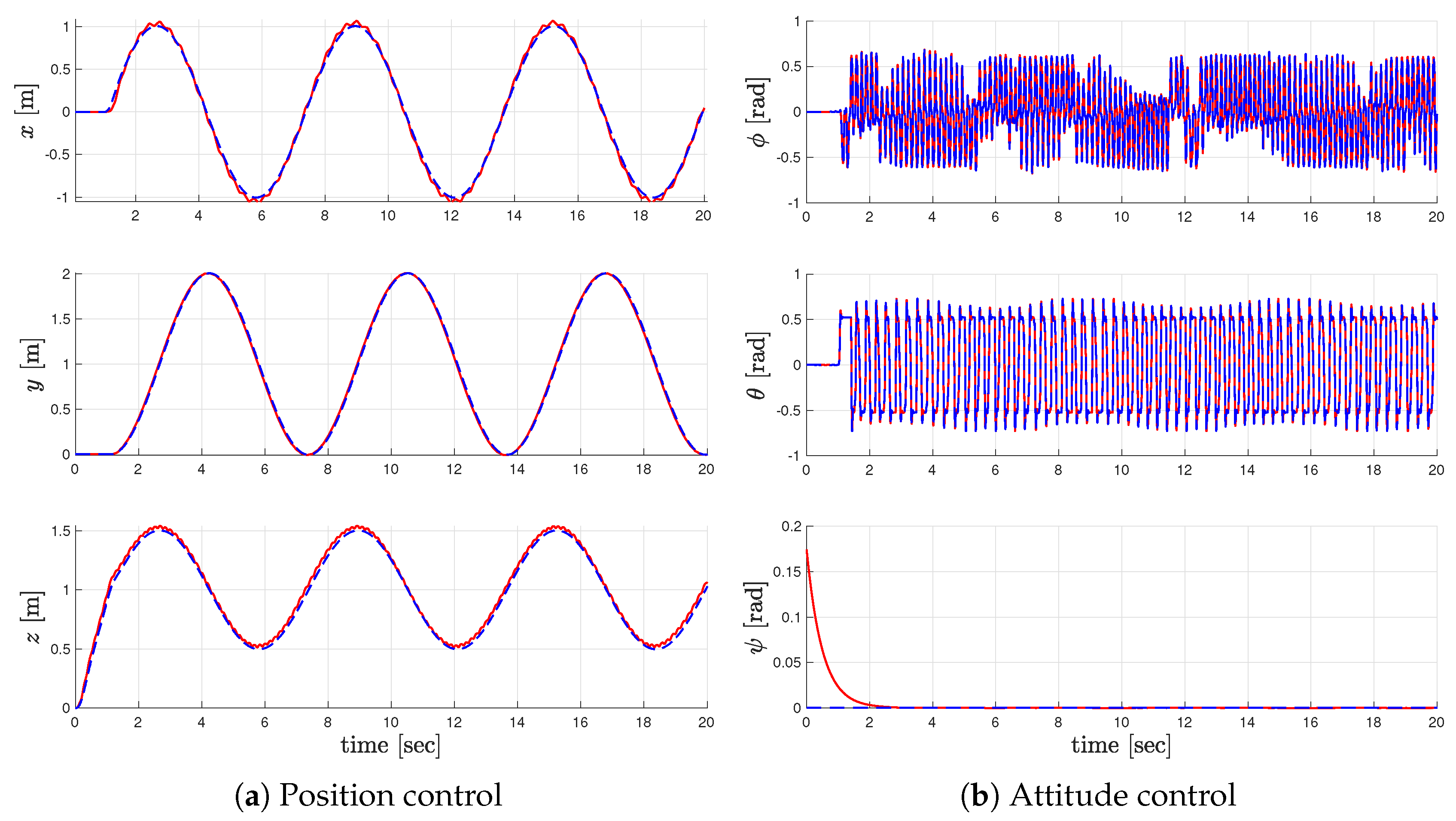
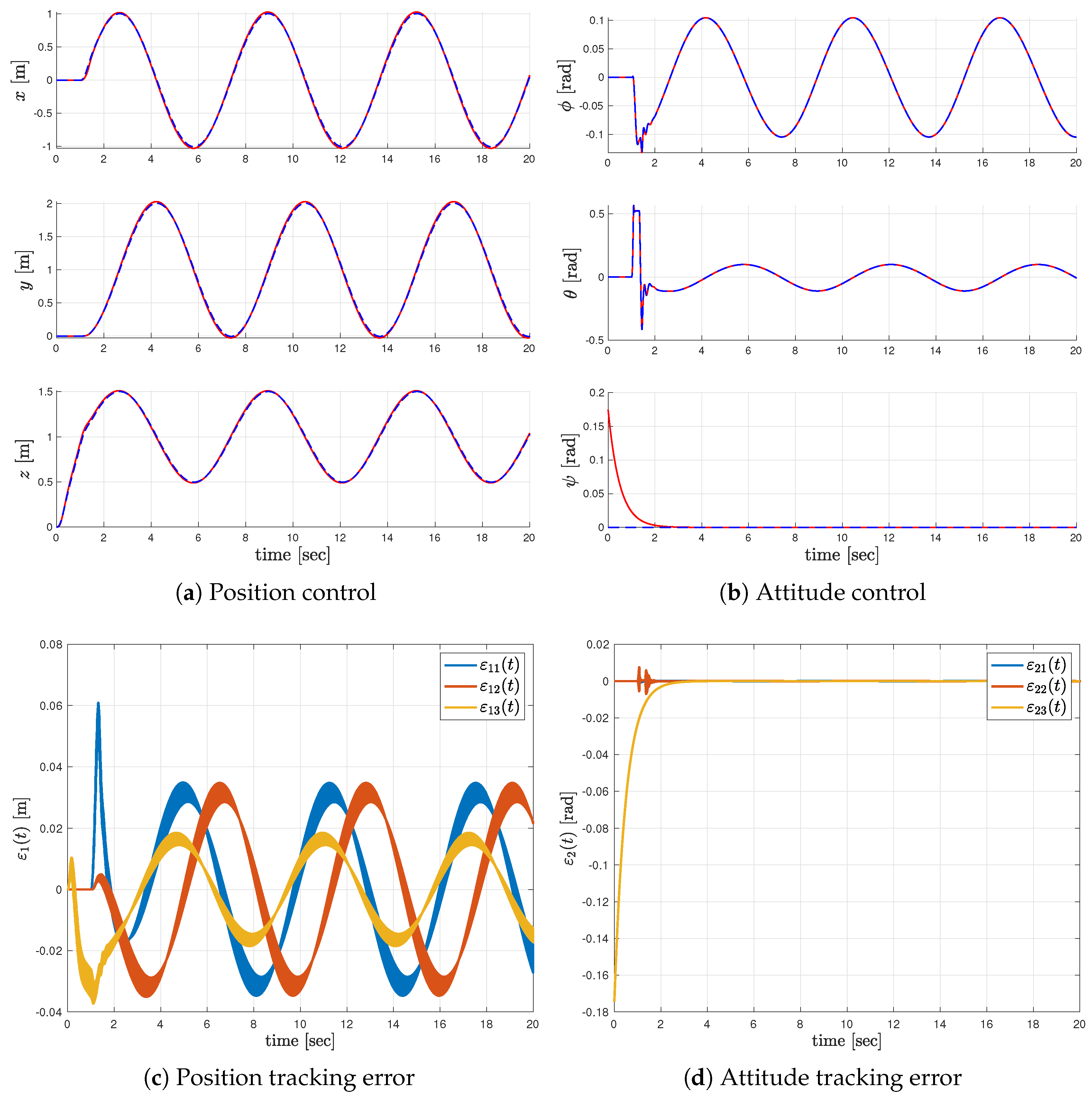
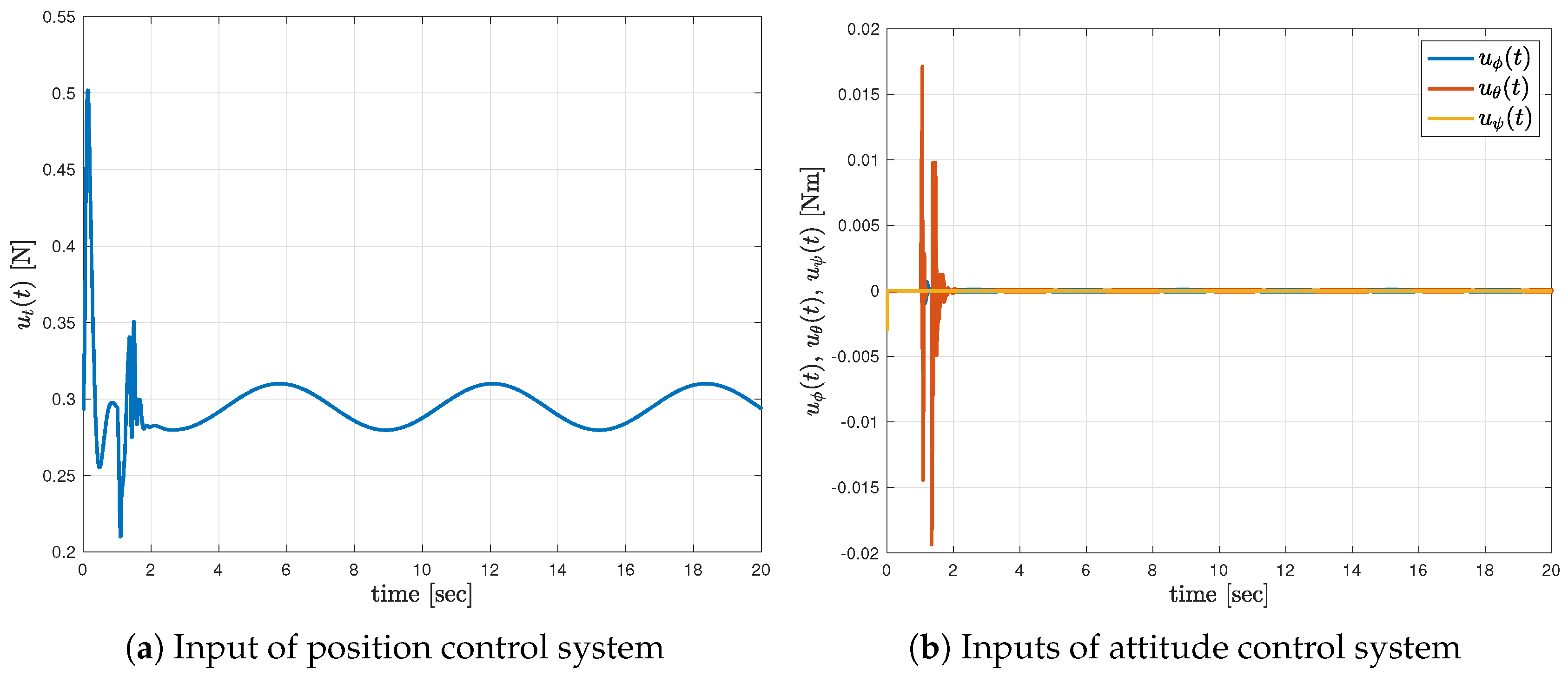
4. Simulation Examples

In the simulation, we employed the quadrotor model mimicking the Crazyflie quadrotor shown in Figure 1. Considering the configuration of the body and inertial axes depicted in Figure 1, the relationships between the rotor thrust and control inputs to each axis are formulated as follows:

$$\begin{array}{cc}\hfill u_t\left(t\right)& =T_1\left(t\right)+T_2\left(t\right)+T_3\left(t\right)+T_4\left(t\right),u_{\varphi }\left(t\right)=d\{T_3\left(t\right)+T_4\left(t\right)-T_1\left(t\right)-T_2\left(t\right)\},\hfill \\ \hfill u_{\theta }\left(t\right)& =d\{T_2\left(t\right)+T_3\left(t\right)-T_1\left(t\right)-T_4\left(t\right)\},u_{\psi }\left(t\right)=c_d\{T_2\left(t\right)+T_4\left(t\right)-T_1\left(t\right)-T_3\left(t\right)\},\hfill \end{array}$$

where $T_i\left(t\right)$ with $i\in {\mathcal{I}}_4$ is a thrust force produced by ith rotor in $\left[\mathrm{N}\right]$; d is the length from the center of the quadrotor to the center of each rotor in $\left[\mathrm{m}\right]$; and $c_d$ is a proportional coefficient in $[\mathrm{Nm}/\mathrm{N}]$.

The authors in [46] measured model parameters for the Crazyflie quadrotor, and the results were as follows: $m=0.0299\left[\mathrm{kg}\right]$, $I_x=I_y=1.935\times {10}^{-5}[\mathrm{kg}·{\mathrm{m}}^2]$, $I_z=2.173\times {10}^{-5}[\mathrm{kg}·{\mathrm{m}}^2]$, $d=0.03973\left[\mathrm{m}\right]$, $c_d=0.0251[\mathrm{Nm}/\mathrm{N}]$.

The reference model for the attitude control system was designed as follows:

$$\begin{array}{c}\hfill A_2^r=\left[\begin{array}{cccccc}0& 0& 0& 1& 0& 0\\ 0& 0& 0& 0& 1& 0\\ 0& 0& 0& 0& 0& 1\\ -{10}^4& 0& 0& -{10}^2& 0& 0\\ 0& -{10}^4& 0& 0& -{10}^2& 0\\ 0& 0& -{10}^3& 0& 0& -{10}^2\end{array}\right],B_2^r=\left[\begin{array}{ccc}0& 0& 0\\ 0& 0& 0\\ 0& 0& 0\\ {10}^4& 0& 0\\ 0& {10}^4& 0\\ 0& 0& {10}^4\end{array}\right],\end{array}$$

from which we know that the settling time for the roll and pitch axes is $0.0808\mathrm{s}$, and that for the yaw axis is $0.3592\mathrm{s}$. Securing the control performance of the roll and pitch axes is essential for the horizontal position to be stabilized. Thus, we designed the reference model for the roll and pitch axes to converge faster than that for the yaw axis. In addition, the reference model for the position control system is as follows:

$$\begin{array}{c}\hfill A_1^r=\left[\begin{array}{cccccc}0& 0& 0& 1& 0& 0\\ 0& 0& 0& 0& 1& 0\\ 0& 0& 0& 0& 0& 1\\ -{10}^2& 0& 0& -{10}^1& 0& 0\\ 0& -{10}^2& 0& 0& -{10}^1& 0\\ 0& 0& -{10}^2& 0& 0& -{10}^1\end{array}\right],B_1^r=\left[\begin{array}{ccc}0& 0& 0\\ 0& 0& 0\\ 0& 0& 0\\ {10}^2& 0& 0\\ 0& {10}^2& 0\\ 0& 0& {10}^2\end{array}\right],\end{array}$$

which indicates that the settling time for all axes is $0.8076\mathrm{s}$. Physically, the fast convergence of the horizontal position causes huge changes in roll and pitch angles, so we chose the settling time as a reasonable value.

In this simulation, we also assumed that the quadrotor flied in an indoor environment. Therefore, the position of the quadrotor is measured through an external optical sensor such as Optitrack or VICON. The measured position information is then transmitted to the quadrotor through wireless communication, so the position controller feeds back the delayed information. In this simulation, we assumed that a time delay of up to $30\mathrm{ms}$ occurred.

In addition, the onboard computer of the quadrotor runs the attitude controller at a frequency of $500\mathrm{Hz}$ due to limitations in hardware performance. On the other hand, according to the sample period of the external optical sensor, the position controller operates at $100\mathrm{Hz}$.

Now that we dealt with all the information about the simulation configuration, we find the appropriate gain matrices on the basis of the LMI conditions given in Theorem 2. The simulations were run in MATLAB 2022a, and the LMIs were solved using YALMIP [47] as the interface and MOSEK [48] as the solver. Under $({\alpha }_1,{\beta }_1,{\lambda }_{F_1},{\rho }_1,{\delta }_{1k},h_1,\tau )=(2,50,9.8\times {0.1343}^2,10,0.3,0.01,0.03)$, $({\alpha }_2,{\beta }_2,{\lambda }_{F_2},{\rho }_2,{\delta }_{2k},h_2)=(0.1,50,1,1,0.1,0.002)$, we solved LMIs in Theorem 2. From the solution, we obtained the following gain matrices:

$$\begin{array}{cc}\hfill K_{11}=& \left[\begin{array}{cccccc}-0.9589& -0.0000& -0.0000& -0.5985& -0.0000& 0.0000\\ -0.0000& -0.9589& 0.0000& -0.0000& -0.5985& -0.0000\\ 0.0000& -0.0000& -1.6746& 0.0000& -0.0000& -0.6604\end{array}\right],\hfill \\ \hfill K_{12}=& \left[\begin{array}{cccccc}-0.9589& -0.0000& -0.0000& -0.5985& 0.0000& 0.0000\\ 0.0000& -0.9589& 0.0000& 0.0000& -0.5985& -0.0000\\ 0.0000& -0.0000& -4.1950& -0.0000& 0.0000& -1.6476\end{array}\right],\hfill \\ \hfill K_{21}=& {10}^{-3}\times \left[\begin{array}{cccccc}-10.0526& 0.0013& -0.0004& -9.5376& 0.0002& 0.0001\\ -0.0020& -10.1610& -0.0001& 0.0001& -9.5381& -0.0003\\ -0.0074& 0.0097& -17.1415& -0.0038& -0.0009& -8.5705\end{array}\right],\hfill \\ \hfill K_{22}=& {10}^{-3}\times \left[\begin{array}{cccccc}-10.0526& 0.0046& 0.0010& -9.5376& 0.0022& 0.0009\\ -0.0053& -10.1610& 0.0003& -0.0019& -9.5380& -0.0001\\ 0.0040& -0.0058& -17.1076& 0.0055& -0.0006& -8.5526\end{array}\right],\hfill \\ \hfill K_{23}=& {10}^{-3}\times \left[\begin{array}{cccccc}-10.0525& -0.0037& 0.0002& -9.5376& -0.0019& 0.0004\\ 0.0027& -10.1609& -0.0005& 0.0022& -9.5380& -0.0005\\ -0.0054& -0.0065& -17.1069& -0.0022& -0.0009& -8.5527\end{array}\right],\hfill \\ \hfill K_{24}=& {10}^{-3}\times \left[\begin{array}{cccccc}-10.0525& -0.0001& 0.0003& -9.5375& 0.0001& 0.0006\\ -0.0006& -10.1610& 0.0003& 0.0002& -9.5381& -0.0001\\ 0.0020& -0.0038& -17.0993& 0.0049& -0.0007& -8.5478\end{array}\right].\hfill \end{array}$$

By using the gain matrices above, we simulated the quadrotor tracking control. The objective of the control is to make the system’s state trajectory follow the reference model’s state trajectory. We plotted the state responses of both the system and the reference model in Figure 2a,b. In addition, the time responses of the tracking errors are shown in Figure 2c,d. Moreover, the time responses of the control inputs for control systems are depicted in Figure 3. The position- and attitude-control systems both achieved the control objective. The proposed controller also robustly controlled the system despite the $30\mathrm{ms}$ time delay.

To investigate the effect of considering the time delay in the controller design, we obtained the position control gain under $\tau =0.001$, which means that the designed controller did not compensate for the communication delay in the position control system. The results are as follows:

$$\begin{array}{cc}\hfill K_{11}=& \left[\begin{array}{cccccc}-2.9403& -0.0000& 0.0000& -1.1309& -0.0000& -0.0000\\ -0.0000& -2.9403& 0.0000& -0.0000& -1.1309& 0.0000\\ 0.0000& -0.0000& -7.6251& 0.0000& -0.0000& -2.1314\end{array}\right],\hfill \\ \hfill K_{12}=& \left[\begin{array}{cccccc}-2.9398& 0.0000& 0.0000& -1.1306& 0.0000& -0.0000\\ 0.0000& -2.9398& 0.0000& 0.0000& -1.1306& 0.0000\\ 0.0000& -0.0000& -11.3024& 0.0000& -0.0000& -2.9625\end{array}\right].\hfill \end{array}$$

Using the above gain matrices, we depict the corresponding position and attitude state trajectories in Figure 4. Compared with Figure 2, the control result in Figure 4 shows that the control performance was degraded by the disturbance caused by the communication delay of position information. Due to the delayed position information, an abrupt change occurred in the output of the position controller. Therefore, the state trajectory of the attitude control system oscillated very quickly.

Table 1. Quantitative comparison of position tracking performance according to $\tau$.

	Maximum Absolute Error			RMS Error
	$\mathit{x}\left[\mathbf{m}\right]$	$\mathit{y}\left[\mathbf{m}\right]$	$\mathit{z}\left[\mathbf{m}\right]$	$\mathit{x}\left[\mathbf{m}\right]$	$\mathit{y}\left[\mathbf{m}\right]$	$\mathit{z}\left[\mathbf{m}\right]$
$\tau =0.03$	0.0609	0.0351	0.0373	0.0181	0.0187	0.0113
$\tau =0.001$	0.1131	0.4170	0.7520	0.0298	0.0188	0.0306

provides the quantitative analysis results of the control performance considering the communication delay. We measured two performance indices: the maximal absolute error and the root mean squared (RMS) error between the system and reference models. Table 1 shows that the proposed control design technique effectively enhanced the control performance when the communication delay occurred in the position control system.

5. Conclusions and Future Works

Considering the communication delay, the decentralized sampled-data fuzzy tracking control method of a quadrotor UAV was proposed. Since the communication delay only occurs in information related to the position of the quadrotor UAV, it was necessary to separate the control system into position and attitude. In this regard, decentralized T–S fuzzy modeling was introduced with a novel decentralized controller. In addition, in order to reduce the computational complexity, an LKF including only the necessary information for each control system was constructed. All conditions derived in this study were represented in terms of LMIs and numerically solved, and the validity and feasibility of the proposed method were verified through the provided simulation examples.

On the other hand, the effectiveness and validity of the method proposed in this study were verified only through the simulation examples. Therefore, our future work is to extend the study to empirical verification taking into account external disturbances and quantization errors.

References

1. Idrissi, M.; Salami, M.; Annaz, F. A Review of quadrotor unmanned aerial vehicles: Applications, architectural design and control algorithms. J. Intell. Robot Syst. 2022, 104, 22. [Google Scholar] [CrossRef]
2. Salih, A.L.; Moghavvemi, M.; Mohamed, H.A.F.; Gaeid, K.S. Modelling and PID controller design for a quadrotor unmanned air vehicle. In Proceedings of the IEEE International Conference on Automatation, Quality and Testing, Robotics (AQTR), Cluj-Napoca, Romania, 28–30 May 2010; pp. 1–5. [Google Scholar]
3. Li, J.; Li, Y. Dynamic analysis and PID control for a quadrotor. In Proceedings of the IEEE International Conference on Mechatronics and Automation, Beijing, China, 7–10 August 2011; pp. 573–578. [Google Scholar]
4. Gaicia, R.A.; Rubio, F.R.; Ortega, M.G. Robust PID control of the quadrotor helicopter. IFAC Proc. 2012, 45, 229–234. [Google Scholar]
5. Zhang, X.; Chen, C.; Su, K.; Lin, L.; Tian, Y. Design of the outdoor cruising control system of the quadrotor drone. IOP Conf. Ser. Earth Environ. Sci. 2021, 632, 022062. [Google Scholar] [CrossRef]
6. Bouabdallah, S.; Noth, A.; Siegwart, R. PID vs LQ control techniques applied to an indoor micro quadrotor. In Proceedings of the IEEE/RSJ International Conference on Intelligent Robots and Systems, Sendai, Japan, 28 September–2 October 2004; pp. 2451–2456. [Google Scholar]
7. Castillo, P.; Lozano, R.; Dzul, A. Stabilization of a mini rotorcraft with four rotors. IEEE Control Syst. Mag. 2005, 25, 44–55. [Google Scholar]
8. Reyes-Valeria, E.; Enriquez-Caldera, R.; Camacho-Lara, S.; Guichard, J. LQR control for a quadrotor using unit quaternions: Modeling and simulation. In Proceedings of the 23rd International Conference on Electronics, Communications and Computing (CONIELECOMP), Cholula, Puebla, Mexico, 11–13 March 2013; pp. 172–178. [Google Scholar]
9. Zhao, S.; An, H.; Zhang, D.; Shen, L. A new feedback linearization LQR control for attitude of quadrotor. In Proceedings of the 13th International Conference on Control Automation Robotics & Vision (ICARCV), Singapore, 10–12 December 2014; pp. 1593–1597. [Google Scholar]
10. Wang, B.; Zhang, Y.; Zhang, W. Integrated path planning and trajectory tracking control for quadrotor UAVs with obstacle avoidance in the presence of environmental and systematic uncertainties: Theory and experiment. Aerosp. Sci. Technol. 2022, 120, 107277. [Google Scholar] [CrossRef]
11. Raffo, G.V.; Ortega, M.G.; Rubio, F.R. Backstepping/nonlinear H control for path tracking of a quadrotor unmanned aerial vehicle. In Proceedings of the American Control Conference (ACC2008), Seattle, WA, USA, 11–13 June 2008; pp. 3356–3361. [Google Scholar]
12. Yu, G.; Cabecinhas, D.; Cunha, R.; Silvestre, C. Nonlinear backstepping control of a quadrotor-slung load system. IEEE/ASME Trans. Mechatron. 2019, 24, 2304–2315. [Google Scholar] [CrossRef]
13. Almakhles, D.J. Robust backstepping sliding mode control for a quadrotor trajectory tracking application. IEEE Access 2019, 8, 5515–5525. [Google Scholar] [CrossRef]
14. Xu, L.-X.; Ma, H.-J.; Guo, D.; Xie, A.-H.; Song, D.-L. Backstepping sliding-mode and cascade active disturbance rejection control for a quadrotor UAV. IEEE/ASME Trans. Mechatron. 2020, 25, 2743–2753. [Google Scholar] [CrossRef]
15. Kim, H.S.; Hwang, S.; Joo, Y.H. Interval type-2 fuzzy-model-based fault-tolerant sliding mode tracking control of a quadrotor UAV under actuator saturation. IET Control Theory Appl. 2020, 14, 3663–3675. [Google Scholar] [CrossRef]
16. Lian, S.; Meng, W.; Lin, Z.; Zheng, J.; Li, H.; Lu, R. Adaptive attitude control of a quadrotor using fast nonsingular terminal sliding mode. IEEE Trans. Ind. Electron. 2021, 69, 1597–1607. [Google Scholar] [CrossRef]
17. Huang, S.; Yang, Y. Adaptive neural-network-based nonsingular fast terminal sliding mode control for a quadrotor with dynamic uncertainty. Drones 2022, 6, 206. [Google Scholar] [CrossRef]
18. Nguyen, N.P.; Park, D.; Ngoc, D.N.; Xuan-Mung, N.; Huynh, T.T.; Nguyen, T.N.; Hong, S.K. Quadrotor formation control via terminal sliding mode approach: Theory and experiment results. Drones 2022, 6, 172. [Google Scholar] [CrossRef]
19. Elmokadem, T.; Savkin, A.V. A method for autonomous collision-free navigation of a quadrotor UAV in unknown tunnel-like environments. Robotica 2022, 40, 835–861. [Google Scholar] [CrossRef]
20. Yacef, F.; Bouhali, O.; Khebbache, H.; Boudjema, F. Takagi–Sugeno model for quadrotor modelling and control using nonlinear state feedback controller. Int. J. Control Theory Comput. Model. 2012, 2, 9–24. [Google Scholar] [CrossRef]
21. Lee, H.; Kim, H.J. Robust control of a quadrotor using Takagi–Sugeno fuzzy model and an LMI approach. In Proceedings of the 14th International Conference on Control, Automation and Systems (ICCAS 2014), Seoul, Korea, 22–25 October 2014; pp. 270–374. [Google Scholar]
22. Fu, C.; Sarabakha, A.; Kayacan, E.; Wagner, C.; John, R.; Garibaldi, J.M. Input uncertainty sensitivity enhanced nonsingleton fuzzy logic controllers for long-term navigation of quadrotor UAVs. IEEE/ASME Trans. Mechatron. 2018, 23, 725–734. [Google Scholar] [CrossRef]
23. Kim, D.W. Fuzzy model-based control of a quadrotor. Fuzzy Sets Syst. 2019, 371, 136–147. [Google Scholar] [CrossRef]
24. Zeghlache, S.; Djerioui, A.; Benyettou, L.; Benslimane, T.; Mekki, H.; Bouguerra, A. Fault tolerant control for modified quadrotor via adaptive type-2 fuzzy backstepping subject to actuator faults. ISA Trans. 2019, 95, 330–345. [Google Scholar] [CrossRef] [PubMed]
25. Zhang, X.; Wang, Y.; Zhu, G.; Chen, X.; Li, Z.; Wang, C.; Su, C.-Y. Compound adaptive fuzzy quantized control for quadrotor and its experimental verification. IEEE Trans. Cybern. 2020, 51, 1121–1133. [Google Scholar] [CrossRef]
26. Chen, Q.; Tao, M.; He, X.; Tao, L. Fuzzy adaptive nonsingular fixed-time attitude tracking control of quadrotor UAVs. IEEE Trans. Aerosp. Electron. Syst. 2021, 57, 2864–2877. [Google Scholar] [CrossRef]
27. Kim, H.S.; Lee, K.; Joo, Y.H. Decentralized sampled-data fuzzy controller design for a VTOL UAV. J. Franklin Inst. 2021, 358, 1888–1914. [Google Scholar] [CrossRef]
28. Takagi, T.; Sugeno, M. Fuzzy identification of systems and its applications to modeling and control. IEEE Trans. Syst. Man Cybern. Syst. 1985, SMC-15, 116–132. [Google Scholar] [CrossRef]
29. Kim, H.S.; Lee, K. Sampled-data fuzzy observer design for nonlinear systems with a nonlinear output equation under measurement quantization. Inf. Sci. 2021, 575, 248–264. [Google Scholar] [CrossRef]
30. Tanaka, K.; Wang, H.O. Fuzzy Control Systems Design and Analysis; John Wiley & Sons: Hoboken, NJ, USA, 2004. [Google Scholar]
31. Liu, Y.; Park, J.H.; Gua, B.-Z. Further results on stabilization of chaotic systems based on fuzzy memory sampled-data control. IEEE. Trans. Fuzzy Syst. 2017, 26, 1040–1045. [Google Scholar] [CrossRef]
32. Liu, Y.; Xia, J.; Meng, B.; Song, X.; Shen, H. Extended dissipative synchronization for semi-Markov jump complex dynamic networks via memory sampled-data control scheme. J. Franklin Inst. 2020, 357, 10900–10920. [Google Scholar] [CrossRef]
33. Cheng, J.; Zhang, D.; Qi, W.; Cao, J.; Shi, K. Finite-time stabilization of T–S fuzzy semi-Markov switching systems: A coupling memory sampled-data control approach. J. Franklin Inst. 2020, 357, 11265–11280. [Google Scholar] [CrossRef]
34. Zhang, J.; Liu, D.; Ma, Y.; Yu, P. Non-fragile H memory sampled-data state-feedback control for continuous-time nonlinear Markovian jump fuzzy systems with time-varying delay. Inf. Sci. 2021, 577, 214–233. [Google Scholar] [CrossRef]
35. Sharmila, V.; Rakkiyappan, R. Memory sampled-data controller design for interval type-2 fuzzy systems via polynomial-type Lyapunov–Krasovskii functional. IEEE Trans. Syst. Man Cybern. Syst. 2022. [Google Scholar] [CrossRef]
36. Ge, C.; Park, J.H.; Hua, C.; Guan, X. Nonfragile consensus of multiagent systems based on memory sampled-data control. IEEE Trans. Syst. Man Cybern. Syst. 2018, 51, 391–399. [Google Scholar] [CrossRef]
37. Saravanakumar, R.; Amini, A.; Dutta, R.; Cao, Y. Reliable memory sampled-data consensus of multi-agent systems with nonlinear actuator faults. IEEE Trans. Circuits Syst. II Exp. Briefs 2021, 69, 2201–2205. [Google Scholar] [CrossRef]
38. Mu, X.; Gu, Z.; Hua, L. Memory-based event-triggered leader-following consensus for T–S fuzzy multi-agent systems subject to deception attacks. J. Franklin Inst. 2022, 359, 599–618. [Google Scholar] [CrossRef]
39. Koo, G.B.; Park, J.B.; Joo, Y.H. Decentralized sampled-data fuzzy observer design for nonlinear interconnected systems. IEEE Trans. Fuzzy Syst. 2016, 24, 661–674. [Google Scholar] [CrossRef]
40. Kim, H.J.; Park, J.B.; Joo, Y.H. Decentralized H sampled-data fuzzy filter for nonlinear interconnected oscillating systems with uncertain interconnections. IEEE Trans. Fuzzy Syst. 2019, 28, 487–498. [Google Scholar] [CrossRef]
41. Jang, Y.H.; Kim, H.S.; Kim, E.; Joo, Y.H. Decentralized sampled-data H fuzzy filtering with exponential time-varying gains for nonlinear interconnected systems. Inf. Sci. 2022, 609, 1518–1538. [Google Scholar] [CrossRef]
42. Liu, K.; Fridman, E. Wirtinger’s inequality and Lyapunov-based sampled-data stabilization. Automatica 2012, 48, 102–108. [Google Scholar] [CrossRef]
43. Jang, Y.H.; Lee, K.; Kim, H.S. An intelligent digital redesign approach to the sampled-data fuzzy observer design. IEEE. Trans. Fuzzy Syst. 2022. [Google Scholar] [CrossRef]
44. Arino, C.; Sala, A. Extensions to “Stability Analysis of Fuzzy Control Systems Subject to Uncertain Grades of Membership”. IEEE Trans. Syst. Man Cybern. B Cybern. 2008, 38, 558–563. [Google Scholar] [CrossRef] [PubMed]
45. Petersen, I.R. A stabilization algorithm for a class of uncertain linear systems. Syst. Control Lett. 1987, 8, 351–357. [Google Scholar] [CrossRef]
46. Budaciu, C.; Botezatu, N.; Kloetzer, M.; Burlacu, A. On the evaluation of the crazyflie modular quadcopter system. In Proceedings of the 24th IEEE International Conference on Emerging Technologies and Factory Automation (ETFA), Zaragoza, Spain, 10–13 September 2019; pp. 1189–1195. [Google Scholar]
47. Löfberg, J. YALMIP: A Toolbox for Modeling and Optimization in MATLAB. In Proceedings of the CACSD Conference, Taipei, Taiwan, 2–4 September 2004; pp. 284–289. [Google Scholar]
48. Andersen, E.D.; Andersen, K.D. The Mosek Interior Point Optimizer for Linear Programming: An Implementation of Homogeneous Algorithm; Springer: Boston, MA, USA, 2000; pp. 197–232. [Google Scholar]
Figure 1. Crazyflie 2.0 and its coordinate system.
Drones 06 00280 g001
Figure 2. (a,b): state responses of the system (solid red lines) and the reference model (dashed blue lines) that were obtained by the position controller compensating for the time delay; (c,d): time responses of the tracking errors for the position- and attitude-control systems.
Drones 06 00280 g002
Figure 3. Time responses of the control inputs.
Drones 06 00280 g003
Figure 4. State responses of the system (solid red lines) and the reference model (dashed blue lines) that were obtained by the position controller while not compensating for the time delay.
Drones 06 00280 g004